Assessing Classification Accuracy as a Criterion for Evaluating the Performance of Seven Topographic Correction Algorithms in the Trinidad Mountains, Cuba

Abstract

To contribute to SDG-15 about the conservation of terrestrial ecosystems, the effective management of land resources is required. In this respect, determining the land use and cover (LUC) based on remote sensing constitutes a strength. For the Arimao watershed in the province Cienfuegos of Cuba, the main difficulty in determining the LUC is related to the topographic correction in the mountains of Trinidad. This study aims to validate the effectiveness of seven topographic correction methods using classification accuracy as a criterion. For this purpose, the mountain area was cut out on the Landsat-8 OLI image of December 2020, based on its physical–geographical and geological characteristics. Seven topographic correction algorithms were applied: Cosine correction, Improved cosine, C-correction, Minnaert, Minnaert with the slope, including Riano and others by Law, and the Normalization correction. To evaluate their performance, three criteria were used: visual interpretation, statistical analysis, and assessing classification accuracy taking into account eight cover classes. The obtained results showed a higher effectiveness of the Minnaert correction with slope and roughness coefficient k = 0.3, with an overall accuracy of 94.08%. The user and producer accuracies increased the performance for almost all forest classes. For the mountains of Trinidad, the non-forest classes were not affected by the topographic correction, so it was possible to apply the topographic correction algorithms to the entire area. The results have demonstrated the necessity of applying the criterion of accuracy assessment to select the best topographic correction.

1. Introduction

The 2030 Agenda for Sustainable Development was approved in 2015, establishing seventeen SDGs [1]. In Cuba, environmental protection is a priority, with soil degradation, erosion, and forest cover reduction identified as major challenges [2]. According to [3], human activity and land use changes are highlighted as the main causes of accelerated soil erosion, negatively affecting global socio-economic conditions. Contributing to SDG 15, which focuses on terrestrial ecosystem conservation, requires effective land management, including the design and continuous updating of land use and cover (LUC) maps to support informed decision-making.

Among the many applications of remote sensing is the mapping of LUC [4,5]. Remote sensing currently represents a significant strength in the face of the limitations of conventional methods for determining land cover, such as topography and field mapping. These limitations are primarily due to challenges related to the work scale, territorial extent, and surface area coverage [6]. Over the last decades, significant advancements have been made in the Landsat series of satellites, particularly with the launch and operation of Landsat-8 and -9. Furthermore, the availability of historical Landsat images free of charge since 2009, provided by the United States Geological Survey (USGS), has created new opportunities for the international remote sensing community.

For the Arimao watershed, located in the province Cienfuegos, Cuba, only two remote sensing LUC studies have been documented. These studies present limitations in the LUC classes due to the objectives of their designs, which, in one case, focuses exclusively on the vegetation category [7] and, in the other, on coastal ecosystems [8]. Given their national scope and 1:100,000 scale, these maps lack a robust assessment of the reliability of their results, primarily due to the costs and difficulties associated with conducting field surveys. However, they were validated using high-resolution images and other cartographic bases.

To develop a project aimed at obtaining LUC maps through remote sensing, starting with a well-defined land cover class legend and an appropriate selection of satellite images [9] according to the study objectives is essential. The process involves three fundamental steps: First, image preprocessing is performed, including geometric, radiometric, and atmospheric corrections [10], but if the area is mountainous, topographic correction is also required [11]. Second, suitable techniques for land coverage detection are selected [5]. Finally, the classification accuracy is assessed [12].

Topographic correction, also known as topographic normalization, is necessary to compensate for the differences in solar illumination in mountainous areas caused by irregular terrain shapes. This effect causes variations in the reflectance response for similar vegetation or cover types, showing that shaded areas have less reflectance than expected; the opposite is true in sunny areas [13].

A variety of topographic correction algorithms have been proposed in the literature. According to [13], these methods are classified into two main groups: those based on band relationships, which are simpler and do not require additional input data, and those that incorporate a Digital Elevation Model (DEM). This approach assumes that reflectance changes uniformly across all bands, allowing the relationship between them to compensate for topographic effects, provided that atmospheric influences have already been accounted for [14,15,16]. These assumptions are typically flawed due to the strong spectral dependence of atmospheric effects [17]. Additionally, these methods often result in a loss of spectral resolution, particularly when classifying multispectral images [13].

The second category of topographic correction methods is based on modeling the illumination (IL) conditions at the time the image was acquired. This approach requires a DEM with the same resolution as the image to be corrected, which allows an estimate of the variations introduced by the topography for each digital level (DL) [18]. After calculating the IL for the entire image, the normalized plane reflectance of each pixel is estimated using methods that can be grouped into two categories, Lambertian and non-Lambertian, depending on whether they assume that reflectance depends on the observation and incidence angles or not [13]. Among the most used Lambertian methods are the Cosine method proposed by [19] and later modified by [20]. Non-Lambertian methods include the one proposed by [21] to evaluate the roughness of the Moon, which was subsequently modified by [15] to include the slope of the terrain. The empirical–statistical method of [19] assumes a linear correlation between the reflectance of each band and the illumination (IL) and applies the C correction to this empirical approach.

The main difficulty in determining the LUC in mountainous regions is related to topographic correction, as there is no consensus on methods that can be universally applied to any geographical area. Without topographic correction, satellite images of mountainous regions can lead to a significant LUC misclassification [22]. Over the last decades, many authors have compared topographic methods applied to Landsat images [11,13,18,23,24,25,26,27]. However, these evaluations generally focus on eliminating or reducing the topographic effect and do not assess its impact on classification accuracy [28]. Nonetheless, the negative impact of this effect on classification accuracy has been demonstrated in several studies [22,29,30,31].

To support environmental management studies and provide input for hydrological model implementation in the basins of Cienfuegos province, obtaining the LUC of the Arimao watershed through remote sensing is necessary. The main challenge lies in the mountainous area in the south–central part of the basin, which requires topographic correction.

In this context, this study aims to assess the performance of seven topographic correction methods applied in the mountainous region of the Arimao watershed in Cuba, using classification accuracy as a criterion. For this purpose, this study was conducted entirely using free software. The mountainous area was extracted from a Landsat-8 OLI surface reflectance (SR) image, and the performance of the topographic correction methods available in the System for Automated Geoscientific Analyses (SAGA) was evaluated. Three criteria were used to assess performance: visual interpretation, statistical analysis, and supervised classification accuracy across eight land cover classes.

This study could be useful as a reference for conducting a LUC project that requires topographic correction. Furthermore, it contributes to systematizing a methodology for the study area that could be applied in other geographic zones.

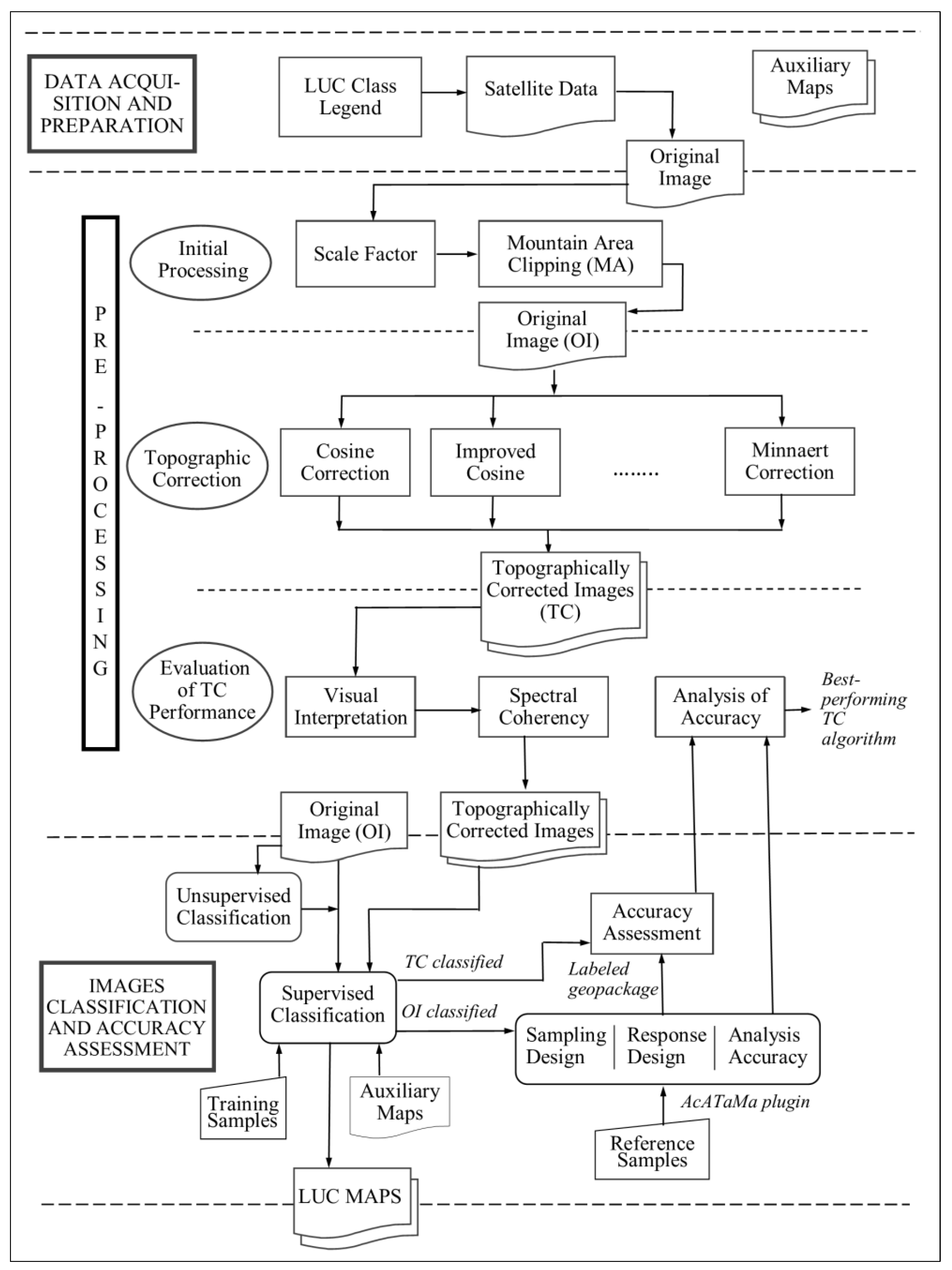
2. Materials and Methods

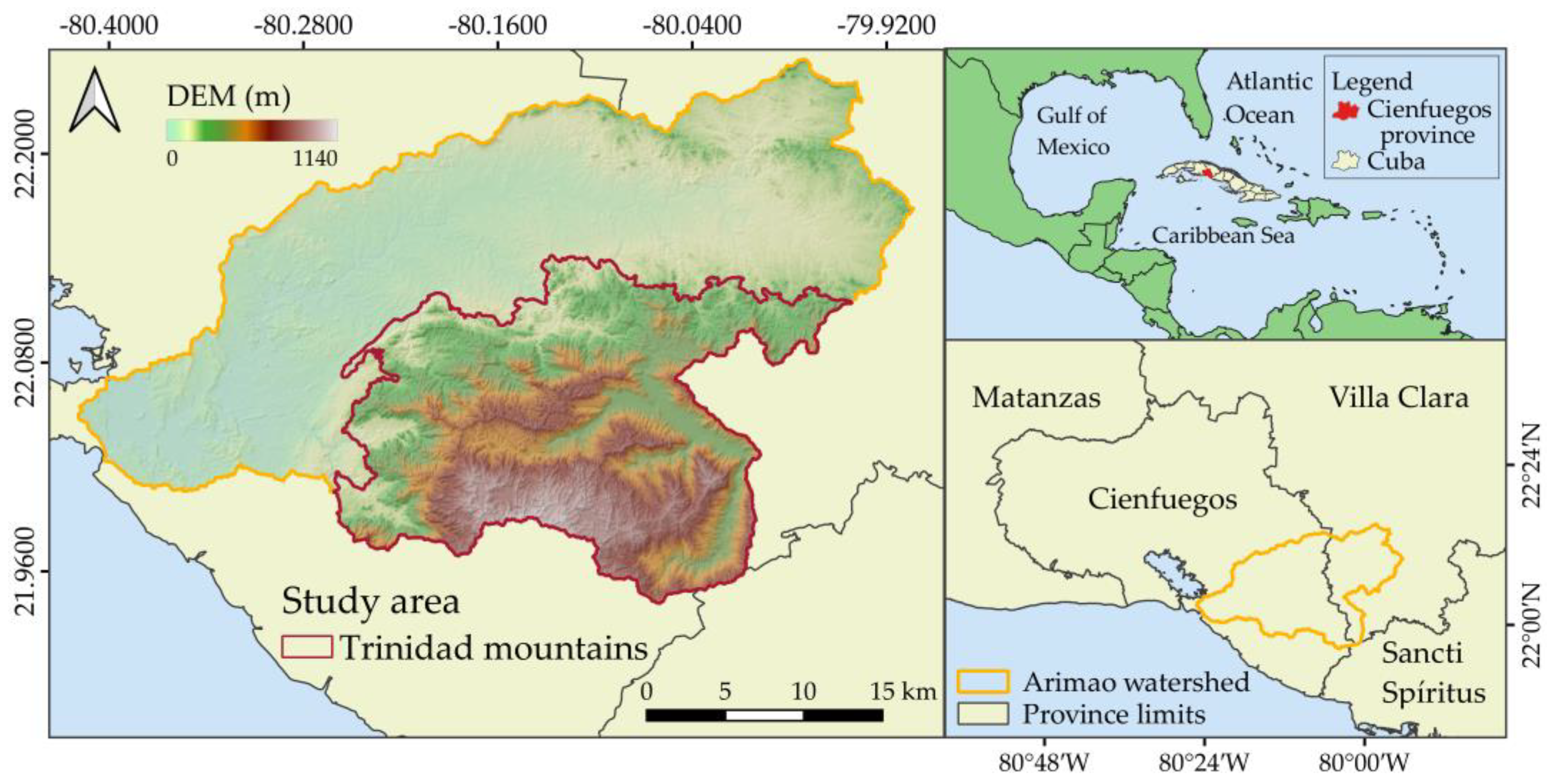
2.1. Study Area

Cuba is an archipelago located in the western part of the Antillean arch. A natural central dividing line runs along the national territory, separating it into northern and southern slopes. Cuba’s climate is warm, tropical and seasonally humid, and is influenced by maritime conditions [32].

Guamuhaya is the mountainous system located in the central geomorphological region of Cuba. It spans the provinces of Sancti Spíritus, Villa Clara, and Cienfuegos, covering an area of 2700 km² [33]. The terrain is highly complex, characterized by dome–block mountains divided into three main blocks: the Trinidad Mountains to the west, the Sancti Spíritus Mountains to the east, and the Agabama Valley in between [34]. This classification defines three morphometric levels within the Trinidad Mountain block: pre-mountains (300–500 m), small mountains (500–1000 m), and low mountains (1000–1500 m). This region features pronounced relief, with San Juan Peak reaching 1140 m above sea level [33].

The Arimao watershed (Figure 1) spans 1006 km², with 413.9 km² occupied by the Trinidad Mountains in the south–central region. The watershed consists of two main morphological units: the Arimao depression (or plain) and the Trinidad Mountains. This study focuses specifically on the mountainous region, where slopes range from 0° to 60°, with an average of 9.7°. Geographically, the area is highly diverse due to the complex geological and geomorphological processes shaping its evolution. Lithologically, the Trinidad Mountains are predominantly composed of metamorphic rocks of varying ages, mainly metaterrigenous and metacarbonate rocks, with lesser amounts of metavolcanic rocks, primarily amphibolites from the Mabujina Complex [35]. Precipitation exhibits strong seasonality, with a rainy period from May to October, accounting for approximately 80% of the annual total, and a least rainy period from November to April. The average annual rainfall is 1608 mm [36]. The average temperature measured in a sector of the Trinidad Mountains is 21.29 °C, ranging from 17.1 °C to 27.2 °C, while the average relative humidity is 74.17%, with values between 55% and 88% [37].

This study proposes a methodology that integrates the use of remote sensing with the Geographic Information System (GIS) QGIS version 3.22.5 Białowieża for image processing and SAGA version 8.5.0 [38], which was selected for topographic correction using its seven available algorithms. The methodology, outlined in Figure 2, comprises three fundamental stages:

• Data acquisition and preparation—This initial stage involves acquiring and preparing numerical and geographic data, selecting the land user/cover legend, and downloading of the satellite images.
• Image pre-processing—In this stage, a scale factor was applied to all image bands. Additionally, seven topographic correction algorithms were implemented for the mountainous region and their accuracy was evaluated using various criteria.
• Images classification and accuracy assessment—The final stage begins with an unsupervised classification of the image that yielded the best spectral coherence. Preliminary results from these classifications were used to select training samples for supervised classification of the topographically corrected images. The accuracy of classification was assessed, and based on the results, the optimal topographic correction algorithm and land cover map were selected.

2.2. Data Acquisition and Preparation

2.2.1. Define the LUC Legend

To define the LUC legend, the second land cover classes legend of Cuba [39] and the classification of the study area by [7] were used. Although [7] identified mountain rainforests between 800 and 1600 m in the study area, this forest type is no longer found in pure patches.

The extent of the original rainforest began to decrease in the 1940s, driven by government policies promoting coffee cultivation. This decline was further exacerbated in the 1960s and 1970s when non-native species were introduced into reforestation programs. These included Pinus caribeae (conifers), Eucalyptus sp., and Swietenia sp. Currently, only coniferous areas remain representative, as other species failed to survive extreme meteorological conditions such as droughts and hurricanes. The establishment of four protected areas and a biological corridor within the watershed has promoted the recovery of evergreen mesophyll forests and rainforests, with noticeable patches expected to reemerge soon.

Based on the classes of interest for hydrological modeling and environmental management studies in the Arimao watershed, a legend consisting of eight land cover classes was proposed: Class 1, Water surface (WS); Class 2, Infrastructure (IS); Class 3, Grassland (GL); Class 4, Bare soil (BS); Class 5, Secondary scrub (SS); Class 6, Secondary forest (SF); Class 7, Mesophyll evergreen forest (EF); and Class 8, Coniferous forest (CF).

2.2.2. Selection and Download of Landsat Images

The selection of the acquisition date considered cloud cover, climatic conditions, and a representative phenological phase, as well as the availability of consistent data. Landsat-8 OLI images (path 14, row 45) from 2020 were reviewed using the USGS Earth Explorer portal. The selected image Collection 2, Level 2 was acquired on 13 December 2020 (LC08_L2SP_014045_20201213_20201219_02_T1), with a 30 m spatial resolution and includes seven surface reflectance (SR) bands. The solar geometry parameters are a sun azimuth of 152.99° and sun elevation of 40.20°. This image is suitable for analysis because, in December, the less rainy season is not fully established and the relative humidity remains high. No significant phenological changes occurred in the forests of the Trinidad Mountains during this period. Despite a 6.32% cloud cover, the mountainous region of the Arimao watershed remained cloud-free. The selected image was rescaled according to the guidelines provided by [40]. This rescaled image is considered equivalent to the original for subsequent analyses.

2.2.3. Auxiliary Geographic Data

The map of natural and semi-natural vegetation of Cuba, with a scale of 1:100,000, was used as auxiliary data [7]. For topographic corrections, the local Digital Elevation Model of 2008 provided by the Geocuba company in Cienfuegos was utilized. This DEM, with a spatial resolution of 26 m, was resampled to 30 m. All geographic data were projected to WGS84/UTM Zone 17N (EPSG: 32617), which uses the World Geodetic System 1984 datum and the UTM projection for Cuba.

2.3. Mountain Area Clipping

Topographic correction methods applied to large areas can present challenges because many correction parameters depend on land cover [18]. Some authors estimate these parameters separately for different types of coverage by applying several algorithms. In the studies by [11,18] a threshold in the NDVI index was used to divide the area into two classes: forest and non-forest. Meanwhile, [41] stratified forest cover into two distinct areas based on slope ranges. Additionally, [13] used a highly detailed vegetation map based on the aerial photographs and fieldwork conducted by the Cabañeros National Park rangers.

In the Arimao watershed, due to its complex physical–geographical features, which are particularly pronounced in the area occupied by the mountains of Trinidad, it was proposed to delimit the mountainous region and apply topographic correction exclusively in this area. This approach also prevents overcorrection in the plain areas of the watershed. To define the mountain limit in the Arimao watershed, all previously mentioned considerations in the study area’s description were taken into account. However, this is a complex task that could benefit from the incorporation of geological criteria (geological structure and lithology) and indices such as the Topographic Position Index (TPI). The process was carried out in two stages: first through desk work, followed by fieldwork.

In the first stage, the 1:100,000 geological map of the study area [42] was consulted, which helped trace the contact limits between the metamorphic rocks and the remaining lithology, generally marked by well-identified geological faults on the map. Afterward, a slope map was generated from the DEM using QGIS and used to calculate the TPI of the watershed. This index allowed for the description of morphological aspects of the terrain and the definition of geomorphological units such as plains, slopes, valleys, and peaks. Additionally, it enabled boundary readjustments considering both geological and geomorphological criteria.

Extensive fieldwork was ultimately conducted, involving sampling throughout the study area, which allowed for a definitive differentiation between the high, hilly surface of the plains from the hills and pre-mountainous heights. The lithology and continuity of the relief were primarily considered, enabling the conclusive establishment of the mountain boundary, characterized by a mean slope of 17°. Using QGIS, this boundary was delimited into six morphometric tiers: small heights (60–100 m), medium heights (100–180 m), high altitudes (180–300 m), sub-mountains (300–500 m), small mountains (500–1000 m), and low mountains (1000–1500 m).

2.4. Topographic Correction Algorithms

Seven topographic correction algorithms available in SAGA (

Table 1. Topographic correction algorithms used in this study.

Correction Algorithms	Equation		Reference
Cosine	${\rho }_H={\rho }_T\left(\cos {\theta }_z/IL\right)$	(2)	[19]
Improved Cosine	${\rho }_H={\rho }_T+\left[{\rho }_i\left({IL}_m-IL/{IL}_m\right)\right]$	(3)	[20]
C Correction *	${\rho }_H={\rho }_T\left(\cos {\theta }_Z+c/IL+c\right)$	(4)	[19]
Minnaert	${\rho }_H={\rho }_T{\left(\cos {\theta }_z/IL\right)}^k$	(5)	[21]
Minnaert of Riano **	${\rho }_H={\rho }_T\cos {\theta }_p{\left(\cos {\theta }_z/IL\cos {\theta }_p\right)}^k$	(6)	[13]
Minnaert of Law ***	${\rho }_H={\rho }_T(\cos {\theta }_p)/({IL}^k{\cos {\theta }_p}^k)$	(7)	[44]
Normalization	${\delta }_{{\rho }_H}={\rho }_T\ast \left[\left[{\rho }_T\left({\mu }_s-X_T\right)/{\mu }_s\right]F_{\lambda }\right]$	(8)	[44]

${\rho }_H$ is the reflectance of the horizontal surface or corrected reflectance and ${\rho }_T$ is the reflectance of the inclined surface or uncorrected reflectance. $c=b/m$, where $c$ is the empirical constant for every band $\lambda$, and $m$ and $b$ are the slope and gradient of regression equation of ${\rho }_T$ versus $IL$. $k$ is the Minnaert constant. ${\delta }_{{\rho }_H}$ is the normalized reflectance data for each pixel in band $\lambda$, ${\mu }_s$ is the mean value for the entire scaled shaded relief model, $X_T$ is the scaled illumination value for each pixel $i$, and $F_{\lambda }$ is the correction coefficient for each band $\lambda$. Abbreviations for algorithm names: * C correction (C-correction), ** Minnaert of Riano (Min-Riano), and *** Minnaert of Law (Min-Law).

) were applied to the mountainous region. These algorithms model the illumination (IL) angle at the time of image acquisition using terrain slope, aspect, and solar–satellite parameters. A DEM is required to compute topographic variations by calculating the solar incidence angle ${\gamma }_i$ for each slope (Equation (1)), which is defined as the angle between the ground normal and the sun’s rays [11,13,20,43]. This angle ranges from −1 to 1, where 1 indicates maximum illumination.

$$IL=\cos {\gamma }_i=\cos {\theta }_z\cos {\theta }_p+\sin {\theta }_z\sin {\theta }_p\cos \left({\phi }_a-{\phi }_0\right)$$

(1)

where ${\theta }_z$ is the solar zenith angle, ${\theta }_p$ is the slope angle, ${\phi }_a$ is the solar azimuth angle, and ${\phi }_0$ is the aspect angle.

Among Lambertian methods, the Cosine algorithm [19] is the most widely used, correcting reflectance based on the solar zenith angle. However, its simplicity leads to an overestimation by ignoring diffuse radiation, particularly in low-illumination areas [13,18,45]. To mitigate this, the Improved cosine, was introduced [20], adjusting the correction based on illumination (IL) levels. The C-correction algorithm [19], by incorporating band-dependent parameters to estimate diffuse irradiance, reduces overcorrection in low-IL regions [31,46,47].

The Minnaert algorithm [21], originally developed to assess lunar surface roughness, is widely used for topographic correction, particularly in forested areas [11,18,48,49]. It employs the Minnaert constant ($k$), a dimensionless empirical parameter ranging from 0 to 1, to characterize surface roughness. A value of $k$ = 1 represents a perfectly Lambertian surface. For this study, $k$ was assigned values of 0.2 and 0.3.

To enhance the satellite image analysis, a modification introduced by [15] incorporates the terrain slope angle ${\theta }_p$, improving the reflectance correction in mountainous areas while keeping $k$ as an empirical parameter. This modified Minnaert with slope method (Min-Riano) was applied by [13] and later incorporated in SAGA. For this study, $k$ values of 0.2, 0.3, and 0.4 were selected to achieve to optimize algorithm performance across the region.

A significant improvement to the original Minnaert algorithm (Min-Law) was introduced by [44], incorporating a non-Lambertian photometric function to reduce overcorrection in shaded areas. While $k$ remained an empirical parameter in that approach, in this study, values of 0.2, 0.3, and 0.4 were assigned. Moreover, they developed the normalization algorithm, a more complex method based on a two-stage approach that applies a broader spectral transformation.

2.5. Performance Evaluation of the Topographic Correction Algorithms

Several criteria have been used in the literature to evaluated the performance of topographic correction algorithms [18,27,30,50]. In this study, the topographically corrected Landsat-8 OLI images were compared with the uncorrected image using three criteria: visual interpretation, statistical analysis and an assessment of classification accuracy.

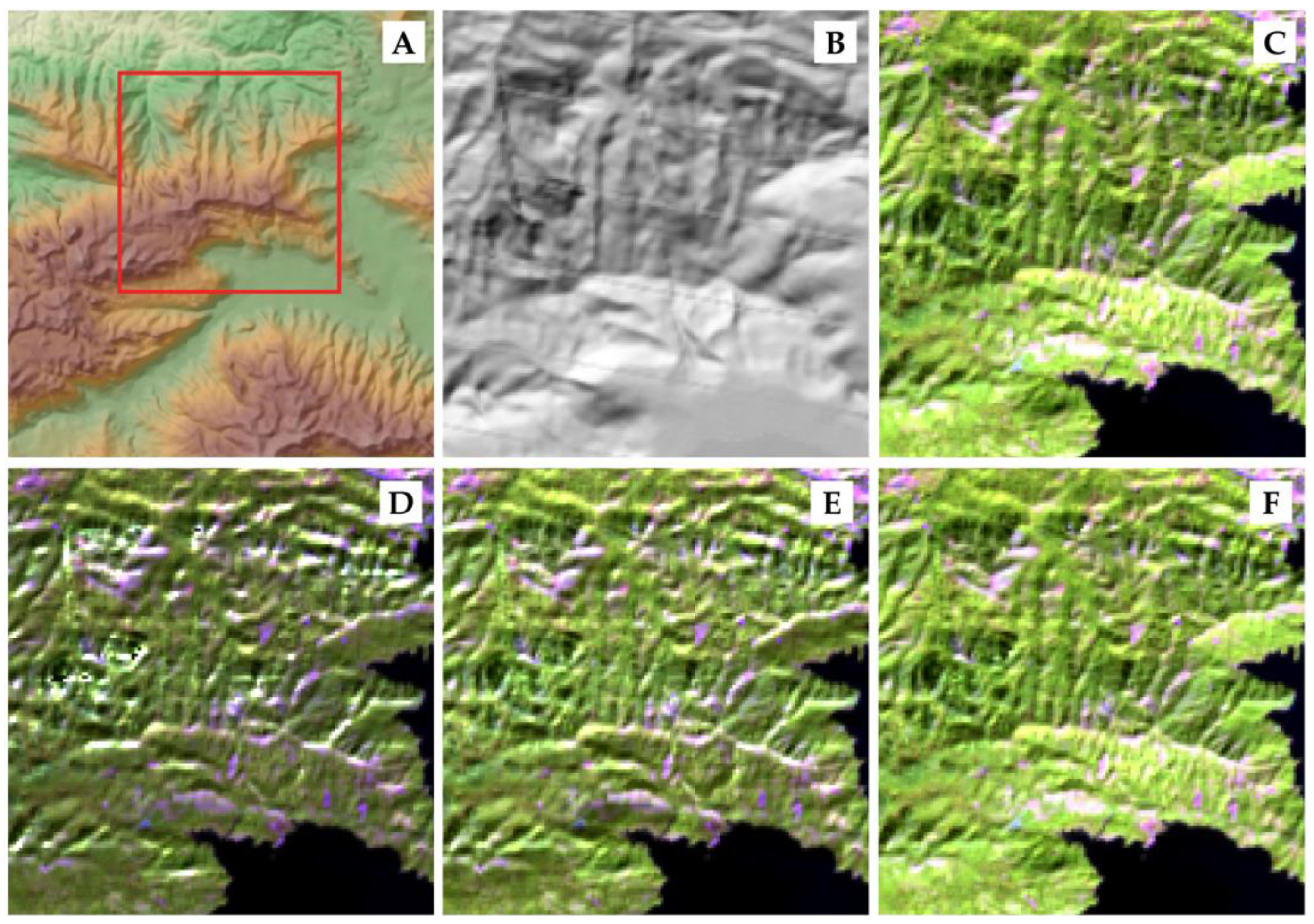
2.5.1. Visual Interpretation

In this criterion, a visual comparison between the topographically corrected images and the original image is performed to evaluate the effect of the correction. In some cases, visual differences between images are evident, indicating over- or under-correction, while in others, they are more subtle. However, the interpretation largely depends on the analyst’s expertise in identifying and discarding low-quality classifications. Visual interpretation has been applied by many authors [11,20,29,41,51].

2.5.2. Spectral Coherence

Spectral coherence can be assessed statistically by analyzing spectral changes after applying different topographic correction algorithms. Many studies compare statistical measures such as the mean ($\mu$) and standard deviation ($\sigma$) of reflectance values between original and corrected images, either for each band individually or as the overall sum of all bands [13,20,41,52]. The μ value represents the average spectral behavior of each band, while σ reflects its internal homogeneity [14].

The coefficient of variation $\left(CV\right)$ has been used to evaluate topographic correction algorithms [11,51,52]. This coefficient is expressed as a percentage and is used to compare variations within datasets, as shown in Equation (9):

$$CV=\left(\sigma /\mu \right)100$$

(9)

According to [11], the $CV$ is expected to decrease after a successful topographic correction. To evaluate this, they propose calculating the differences in CV values across all bands before and after applying the correction algorithms, ensuring a more effective evaluation of the changes, as shown in Equation (10):

$${CV}_{Difference}={CV}_{Beforecorrection}-{CV}_{Aftercorrection}$$

(10)

In this study, the CV difference is calculated for all bands to achieve a better evaluation of the topographic correction algorithms.

2.5.3. Assessing Classification Accuracy

The accuracy assessment is conducted by comparing reference data (ground truth) with the classified map using a confusion matrix and accuracy metrics [53]. This approach is relatively uncommon due to the challenges in ground truth data collection. However, studies [22,30,50] have demonstrated its reliability in evaluating topographic correction algorithms. A detailed description of the accuracy assessment is provided in Section 2.7.

2.6. Classification of Image

2.6.1. Unsupervised Classification

Unsupervised classification of topographically corrected images with the best spectral coherence was performed using ISODATA [54,55] and K-Means [54,55] clustering in QGIS. Kernel signatures were calculated from random pixels based on the Minimum Distance (MD) and Spectral Angle Mapping (SAM) algorithms, using 30 classes and 500 iterations. The K-Means method yielded unsatisfactory results for both algorithms: SAM identified 25 different classes, while MD failed to classify the image. In contrast, ISODATA produced better results, identifying 13 classes with SAM and 9 with MD.

The water surface and grassland classes were the most accurately identified when compared to high-resolution images from Google Earth Pro, dated December 2020. This approach allowed for the identification of clusters corresponding to the legend classes, thus facilitating the extraction of pure pixels before field sampling.

2.6.2. Training Samples (Pure Pixels)

For the supervised classification, 197 training samples were selected. Of these, 24 forest samples were obtained from previous field samplings performed by the Botanical Garden of Cienfuegos in 2018 and 2019. High-resolution images from 2020 on Google Earth Pro were used to obtain 53 training samples of the water surface and 5 samples of infrastructure. The remaining 111 samples were collected during four field samplings conducted between October and December 2020. The samples’ locations were carefully selected to ensure undisturbed areas for each class or pure pixels. The training samples correspond to Mesophyll evergreen forest (24 samples), Coniferous forest (20), Secondary forest (35), Secondary scrub (23), Bare soil (15), Grassland (17), Water surface (53), and Infrastructure (10).

2.6.3. Supervised Classification

For the supervised classification, the methods available in QGIS were analyzed. These include the machine learning algorithms Random Forest (RF) and Support Vector Machine (SVM), as well as traditional classification methods such as Minimum Distance (MD), Maximum Likelihood (ML), and Spectral Angle Mapping (SAM).

Random Forest [56,57] and Support Vector Machine [58,59] are robust classification methods but can be complex, which may be a disadvantage in certain contexts. Their performance depends heavily on parameter tuning, and model accuracy is significantly influenced by the size and balance of training datasets [60,61]. In mountainous areas requiring topographic correction, the MD and ML classification algorithms exhibit several limitations. The MD method is sensitive to illumination variations and does not account for topographic influences [62,63]. On the other hand, the ML method, although widely used, relies on the assumption of Gaussian distributions and is highly sensitive to illumination conditions, making it less effective in mountainous regions [64,65]. The SAM algorithm is less sensitive to topographic effects and illumination changes than other methods, as it relies on the spectral vector’s direction rather than its magnitude. This makes it particularly effective in mountainous areas with significant topographic variation [66,67]. Given these advantages, SAM was selected for the supervised classification of topographically corrected images in the study area.

The classification was carried out using the Semi-Automatic Classification Plugin (SCP) [68] installed in QGIS. Small polygons were digitized around the training data to define the ROIs for each LUC class. The supervised classification was applied to the three topographically corrected images that showed the best results in the statistical analysis of spectral coherence, as well as the original image.

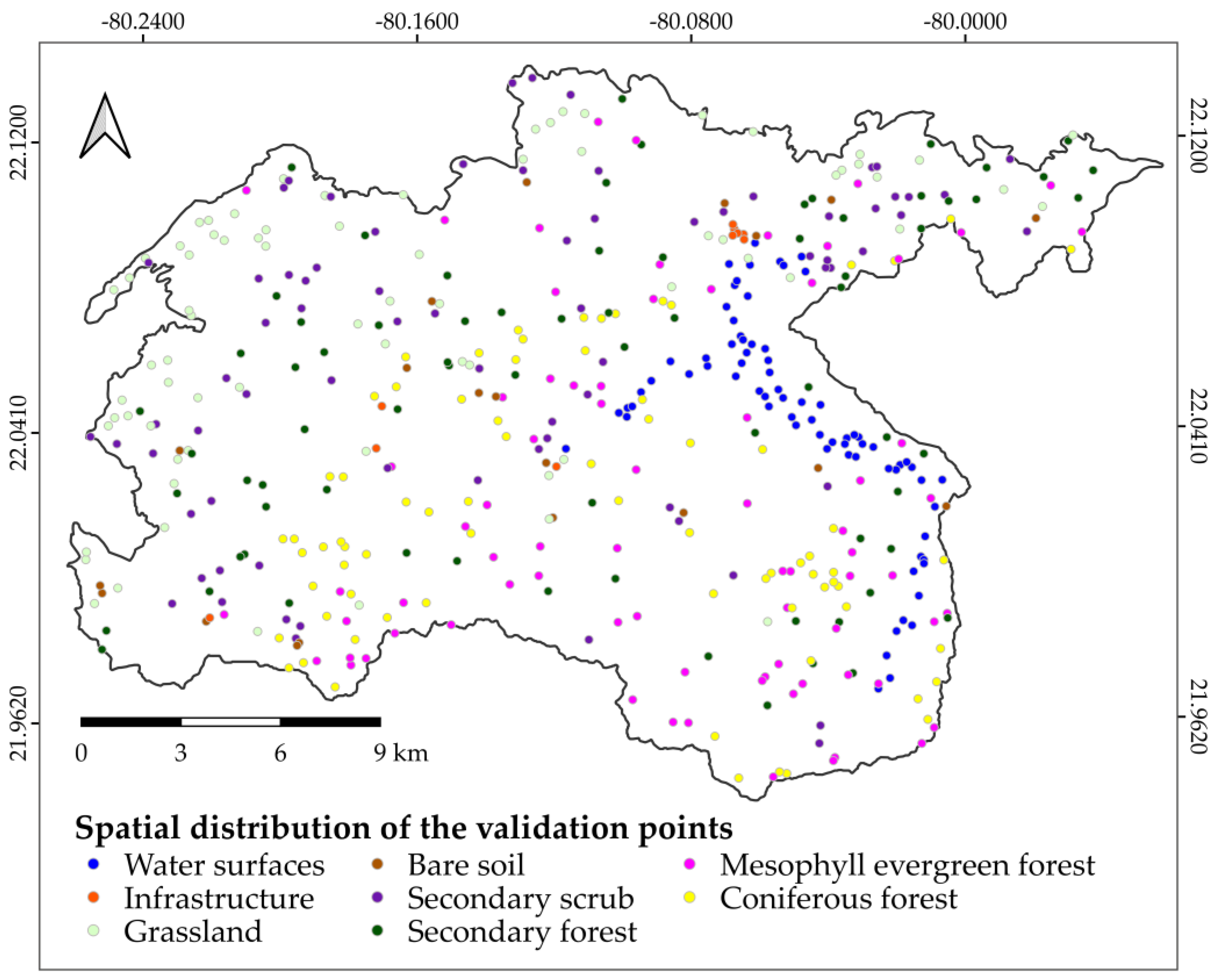
2.7. Imagery Accuracy Assessment

To assess accuracy, a confusion matrix [69,70] was generated using the classified images. Additionally, overall accuracy, user’s accuracy, and producer’s accuracy were calculated [70]. Since the sampling was stratified, the matrix values were adjusted by weighting the number of data points according to the area of each class on the map, using Equation (4) from [71]. Based on this adjusted matrix, global, user, and producer accuracy were computed using Equations (1)–(3) from the same source. Although the Kappa coefficient is widely used [72], it was not calculated, as it is not considered a robust metric [70,73,74,75].

For the accuracy assessment, the classified imagery was compared to higher-quality reference data collected using a sample-based approach. Additionally, it requires defining three fundamental components: the sampling design, the response design, and the accuracy analysis [76].

2.7.1. Sampling Design

The sample size should represent all map classes to ensure a statistically valid accuracy assessment [12]. Determining an appropriate sample size is an iterative process that considers key factors such as resource availability [77], confidence level, and acceptable estimation error [14]. Consequently, there is no single correct method for calculating the sample size [77]. As a general guideline, a minimum of 20 to 100 samples per stratum has been suggested [72,76]. However, for maps covering less than 1 million acres and containing fewer than 12 classes, at least 50 samples per class are commonly recommended [12,78].

In this study, following [11,71,76,79], the eight classes of the classified map described in Section 2.6.3 were selected as strata, and a stratified random sampling approach was used to compute the total sample size for each strata (class). According to [71], for stratified random sampling, the overall sample size $\left(n\right)$ was calculated using the Equation (11):

$$n={\displaystyle \frac{{\left(\sum W_i{S}_i\right)}^2}{{\left[S\left(\widehat{O}\right)\right]}^2+\left(1/N\right)\sum W_i{S_i}^2}}\approx {\left({\displaystyle \frac{\sum W_i{S}_i}{S\left(\widehat{O}\right)}}\right)}^2$$

(11)

where

• $N$ is the number of units in the area of study (number of overall pixels, because the spatial unit is a pixel);
• $S\left(\widehat{O}\right)$ is the standard error of the estimated overall accuracy that we would like to achieve;
• $W_i$ is the mapped proportion of area of stratum $i$;
• $U_i$ is the user’s accuracy estimated for stratum $i$ that we would like to achieve;
• $S_i$ is the standard deviation of the stratum i, $S_i=\sqrt{U_i\left(1-U_i\right)}$;

Equation (11) was implemented in a Microsoft Excel spreadsheet, as proposed by [76] and further improved by the author (Appendix A). All formulas were embedded in the cells, allowing automatic iterations to calculate the overall sample size. For this study, the sample size was computed in the spreadsheet using the original image. Since the overall area is only 458,285 pixels (100,822.70 acres), a minimum sample size of 20 samples per stratum was preferred for the calculation. The target standard error for overall accuracy was set to 0.01, as recommended by [71,76]. The user’s accuracy for all classes was estimated at 0.95 (95%), resulting in a total calculated sample size of 475. Bare soil and infrastructure were considered rare classes due to their minimal areas, covering only 36 and 3.6 hectares (399 and 40 pixels, respectively). The total number of samples was allocated across the classes using four methods: equal allocation, proportional allocation, and two hybrid approaches combining these methods with adjustments for one or two rare strata [71,76]. The sample allocations calculated in Appendix A are shown in

Table 2. Sample size per classes. Water surface (WS), Infrastructure (IS), Grassland (GL), Bare soil (BS), Secondary scrub (SS), Secondary forest (SF), Mesophyll evergreen forest (EF), and Coniferous forest (CF).

Methods/Stratum	WS	IS	GL	BS	SS	SF	EF	CF	Total Samples
Alloc1 (equal)	59	59	59	59	59	59	59	59	475
Alloc2 (proportional)	18	0.04	16	0.5	108	174	143	16	475
Alloc3 (1 rare stratum)	17	20	15	0	104	166	137	15	475
Alloc4 (2 rare stratums)	74	10	74	20	74	74	74	75 *	475

* A total of 74 samples for this class were initially calculated in Appendix A; however, the number was adjusted to 75, bringing the overall total to 475 samples. The sample size for this class was increased due to its large area.

.

The equal (Alloc1) and proportional (Alloc2) methods were suboptimal. In Alloc1, the rare IS class, covering only 40 pixels, received 59 samples—an excessive allocation. Conversely, in Alloc2, five classes had fewer than 20 samples, failing to meet the minimum size criterion. The hybrid Alloc3 prioritized only IS, assigning it a minimum of 20 samples, but left BS with none. Additionally, WS (Water surface), GL (Grassland), and CF (Coniferous forest) had fewer than 20 samples, making this allocation suboptimal as well. The fourth allocation (Alloc4) considered both rare classes, assigning 20 samples to BS and 10 to IS. Sampling approximately one-quarter of their area was deemed sufficient and representative. Alloc4 yielded the best results, balancing proportional and equal allocation methods while ensuring adequate sampling for rare and other classes.

2.7.2. Response Design

The response design was established to assess the agreement between the map and reference data, considering the spatial assessment unit, reference data sources, labeling protocol, and agreement criteria [12,71,76].

In this study, the pixel was chosen as both the spatial assessment unit and the minimum mapping unit (MMU), consistent with the 30 × 30 m resolution of the Landsat image. High-resolution Google Earth Pro (GEPro) images, which are freely available, served as reference data, including an image from 13 December 2020. To define agreement between the map and reference classifications, the simplest approach was adopted [71] using a common classification scheme for both. Under this criterion, a matching label indicates a correct classification, while a mismatch is considered a misclassification.

The thematic accuracy of the classifications was evaluated using version 23.4 of the Accuracy Assessment of Thematic Maps (AcATaMa) plugin for QGIS, designed for validating single LUC maps [80]. Based on the methodologies of [71], it has shown strong performance in studies by various authors [81,82,83,84]. AcATaMa was applied to the classified original image. For the sampling design component, the stratified random sampling method was employed, with fixed values assigned to each category. A total of 475 samples were manually allocated according to the Alloc4 scheme. AcATaMa generated a geopackage containing random points, stratified by classes, which were verified to avoid overlap with those used in the classification. The spatial distribution of the points is shown in Figure 3.

In the response design component, samples were labeled using validation points collected during field surveys (ground truth). Additionally, two supporting data sources were utilized: the Bing satellite base map and the Soil Adjusted Vegetation Index (SAVI). The labeling process was further supported by the expertise of specialists from the Botanical Garden and the Environmental Studies Center of Cienfuegos, whose knowledge of the local mountain environment was invaluable.

2.7.3. Analysis of Accuracy

In the analysis component of the AcATaMa plugin, the stratified estimator was used to compute the confusion matrix, total area, and accuracy metrics, including overall, user’s, and producer’s accuracy, along with their respective standard deviations. Additionally, the confusion matrix and accuracy metrics for the estimated area proportion were calculated. To evaluate the accuracy of the topographically corrected classifications, the same spatial distribution of points generated by the AcATaMa plugin was used to prevent validation bias. However, as the plugin did not permit the reuse of the same geopackage for other maps, this process was performed manually by following the steps outlined below.

The geopackage of points was intersected with the classified map using the ’Point Sampling Tool’ plugin, generating a new geopackage that included a field with the class value from the map, along with the fields previously created by AcATaMa. The ’Match’ field was updated using the field calculator to indicate whether the labeled field corresponded to the thematic class from the map. The geopackage was then exported as a CSV (comma-separated values) file and imported into Microsoft Excel, where a pivot table was used to generate the confusion matrix. Using the same equations applied by the AcATaMa plugin, the other accuracy metrics were calculated. The area of each class was derived from the pixel values in the generated maps, while the adjusted area was calculated by combining the maps with the reference data.

3. Results

The performance of seven topographic correction algorithms was evaluated by comparing the original Landsat-8 OLI image with its topographically corrected versions. The evaluation was based on three criteria: visual interpretation, a statistical analysis of spectral coherence, and an accuracy assessment of supervised classifications. The best algorithm was selected according to the last criterion.

3.1. Visual Interpretation of Topographic Correction Algorithms

Since not all images used for visual interpretation exhibited significant differences, three of the most notable images are shown in Figure 4. The remaining algorithms are shown in Figure S1 of the Supplementary Material. The same location within the study area was selected to display both the original image (Figure 4C) and the topographically corrected images using the local DEM (Figure 4A). The images with the band composition (6-5-4) for the vegetation analysis are shown in Figure 4D–F and Figure S1G–O of the Supplementary Material. The illumination map (Figure 4B) represents the cosine of the solar incident angle, calculated from the image metadata and the DEM. Lighter areas indicate surfaces facing the sun and, therefore, receiving more illumination, while shadowed mountain areas appear darker.

The images corrected using the Cosine (Figure 4D) and C-correction (Figure S1G) algorithms appear overestimated on both sunny and shaded slopes based on a visual interpretation. Compared to the Cosine, the Improved cosine (Figure 4E) exhibited slight overcorrection, possibly due to Lambertian reflectance assumptions. This behavior of cosine-based algorithms has also been reported by [11,13,85]. The Normalization method (Figure S1I) showed a slight overcorrection, similar to the Improved cosine correction.

Of the seven algorithms applied, Minnaert, Min-Riano, and Min-Law (for all $k$ values) (Figure S1) performed best, yielding more homogeneous corrected images. Thus, distinguishing the best result visually was not possible. The visual assessment proved ineffective for selecting the best correction but helped discard the worst results. Consequently, the Cosine and C-correction algorithms were ruled out.

3.2. Statistical Analysis of Spectral Coherence

The original statistical values of the mean (µ), standard deviation (σ), and coefficient of variation (CV) for each band after applying the different topographic correction algorithms are provided in Table S1 of the Supplementary Material.

Table 3. Statistical measures µ, σ (both in percent reflectance), and ${CV}_{Diff}$ between the original image and each applied topographic correction algorithm calculated for each band and the total sum.

Algorithm	Statistic	Band2 Blue	Band3 Green	Band4 Red	Band5 NIR	Band6 SWIR1	Band7 SWIR2	Total Change
Cosine	µ	−0.284	−0.765	−0.431	−7.312	−2.941	−1.202	−12.935
	σ	−5.122	−20.001	−9.005	−222.945	−64.193	−24.897	−346.163
	${CV}_{Diff}$	−329.30	−506.07	−388.40	−588.66	−399.36	−374.87	−2586.66
Improved Cosine	µ	−0.001	−0.004	0.005	−0.003	0.052	0.024	0.074
	σ	−0.042	−0.113	−0.042	−0.705	−0.206	−0.074	−1.181
	${CV}_{Diff}$	−3.398	−3.552	−2.412	−2.336	−1.773	−1.627	−15.100
C-correction	µ	−0.330	−0.857	−0.490	−8.232	−3.355	−1.369	−14.633
	σ	−8.014	−20.416	−11.374	−221.94	−84.708	−32.174	−378.63
	${CV}_{Diff}$	−503.49	−503.96	−479.15	−571.10	−514.82	−473.59	−3046.1
Minnaert k = 0.2	µ	−0.033	−0.086	−0.049	−0.823	−0.337	−0.138	−1.467
	σ	−0.003	0.008	−0.008	0.199	0.060	0.008	0.264
	${CV}_{Diff}$	0.941	1.187	0.963	1.578	1.487	1.334	7.489
Minnaert k = 0.3	µ	−0.053	−0.137	−0.078	−1.312	−0.537	−0.220	−2.337
	σ	−0.014	−0.019	−0.027	0.023	−0.013	−0.027	−0.078
	${CV}_{Diff}$	0.684	0.912	0.766	1.538	1.520	1.366	6.785
Min-Riano k = 0.2	µ	0.020	0.055	0.034	0.548	0.242	0.100	0.997
	σ	0.018	0.060	0.038	0.641	0.272	0.108	1.136
	${CV}_{Diff}$	0.718	1.304	1.120	1.517	1.389	1.178	7.226
Min-Riano k = 0.3	µ	−0.004	−0.010	−0.003	−0.070	−0.013	−0.005	−0.105
	σ	0.007	0.038	0.019	0.508	0.209	0.074	0.855
	${CV}_{Diff}$	0.748	1.315	1.142	1.762	1.668	1.441	8.076
Min-Riano k = 0.4	µ	−0.032	−0.081	−0.044	−0.755	−0.296	−0.121	−1.330
	σ	−0.015	−0.020	−0.017	0.030	0.021	−0.006	−0.007
	${CV}_{Diff}$	−0.093	0.274	0.353	0.955	1.072	0.932	3.493
Min-Law k = 0.2	µ	−0.091	−0.227	−0.130	−2.156	−0.910	−0.375	−3.889
	σ	−0.030	−0.037	−0.047	−0.270	−0.177	−0.109	−0.670
	${CV}_{Diff}$	0.714	1.293	1.119	1.509	1.381	1.172	7.187
Min-Law k = 0.3	µ	−0.178	−0.450	−0.260	−4.304	−1.815	−0.747	−7.755
	σ	−0.067	−0.113	−0.113	−0.909	−0.490	−0.263	−1.955
	${CV}_{Diff}$	0.741	1.302	1.134	1.749	1.657	1.430	8.012
Min-Law k = 0.4	µ	−0.274	−0.696	−0.402	−6.660	−2.807	−1.156	−11.99
	σ	−0.121	−0.237	−0.204	−1.994	−0.968	−0.480	−4.004
	${CV}_{Diff}$	−0.104	0.258	0.340	0.938	1.057	0.920	3.409
Normalization	µ	−0.001	−0.004	0.005	−0.003	0.052	0.024	0.074
	σ	−0.042	−0.113	−0.042	−0.705	−0.206	−0.074	−1.181
	${CV}_{Diff}$	−3.398	−3.552	−2.412	−2.336	−1.773	−1.627	−15.100

presents the percentage reflectance of µ and σ, as well as the difference in the coefficient of variation ($C{V}_{Difference}$ or ${CV}_{Diff}$) for each band after correction. The original image exhibits low CV values in bands 3 and 5, around 35% (Table S1), indicating inherent spectral stability.

According to [20], changes in the spectral characteristics of topographically corrected images should ideally be minimal; significant changes indicate over or under-correction. Statistically, it means that the μ values of each band should be very close to each other [11,22], whereas σ and $CV$ should decrease after applying the correction algorithm and ${CV}_{Diff}$ would have positive values.

Minnaert-based algorithms maintain or slightly enhance spectral coherence, with the blue band consistently showing the lowest ${CV}_{Diff}$ values. In this band, the Improved cosine algorithm has a mean closest to zero (0.001), while the Min-Riano algorithm (k = 0.3) presents a very low mean (0.004) and the lowest standard deviation (0.007), indicating that this band retains the highest spectral coherence. The NIR and SWIR1 bands show higher ${CV}_{Diff}$ values, suggesting that these algorithms are less effective at correcting topographic effects in these bands, leading to more variability.

The Cosine and C-correction methods show extremely high ${CV}_{Diff}$ values (over 400% in some bands), indicating overcorrection and high variability. In contrast, the Improved cosine and Normalization algorithms produce ${CV}_{Diff}$ values closer to the original image, suggesting better spectral coherence. Minnaert-based methods (Minnaert, Min-Riano, and Min-Law) also preserve spectral coherence more effectively than Cosine and C-correction.

The Improved cosine, Normalization, and Min-Riano (k = 0.3) algorithms exhibited the smallest changes in µ after correction, with values of 0.074 for the first two and −0.105 for Min-Riano. In contrast, the Cosine and Min-Law corrections for all k values yielded the worst µ results.

The Minnaert, Min-Riano, and Min-Law algorithms for all coefficients $k$ revealed that they were able to reduce ${CV}_{Aftercorrection}$. As a result, ${CV}_{Diff}$ showed positive values, indicating an improvement in performance. However, despite this, the Minnaert (k = 0.3), Min-Riano (k = 0.4), and Min-Law algorithms increased inter-band variability and presented negative values of σ. Concerning the standard deviation (σ), only the Min-Riano algorithm (k = 0.2 and k = 0.3) reduced its value across all bands. Most topographic correction algorithms increased σ, negatively impacting band homogeneity. The methods that most effectively reduced σ variability were Minnaert (k = 0.2) and Min-Riano (k = 0.2 and k = 0.3). Meanwhile, the worst results were observed for the Cosine and C-correction algorithms, as previously shown by the visual criterion.

The best results for spectral coherence were obtained with Minnaert (k = 0.2) and Min-Riano (k = 0.2 and k = 0.3). These classified images were then used for the accuracy assessment, which is explained in the following section.

3.3. Accuracy Assessment of Classified Images

The results of overall accuracy (OA), based on the error matrices (Tables S2, S4, S6 and S8 in the Supplementary Material), were 91.79% for the original image, 94.95% for the Minnaert (k = 0.2) topographic correction, and 94.11% and 95.16% for the Min-Riano algorithms (k = 0.2 and k = 0.3), respectively. However, when the OA (

Table 4. Classification accuracy assessment of the original image and the topographically corrected images using the Minnaert (k = 0.2) and Min-Riano (k = 0.3 and k = 0.2) algorithms. Producer’s accuracy (PA), user’s accuracy (UA), and overall accuracy (OA) values are expressed as percentages (%).

LUC Classes	Original Image			Minnaert (k = 0.2)
	UA	PA	OA	UA	PA	OA
Water surface	100.00	68.06	89.47	97.37	100.00	92.10
Infrastructure	100.00	100.00		100.00	100.00
Grassland	96.00	99.86		100.00	91.67
Bare soil	90.00	64.15		100.00	67.26
Secondary scrub	93.42	93.45		93.42	97.91
Secondary forest	85.90	91.39		90.00	95.19
Mesophyll evergreen forest	89.19	92.70		92.00	94.82
Coniferous forest	85.92	57.42		95.45	45.85
LUC Classes	Min-Riano (k = 0.2)			Min-Riano (k = 0.3)
	UA	PA	OA	UA	PA	OA
Water surface	97.37	100.00	91.58	100.00	90.02	94.08
Infrastructure	100.00	100.00		100.00	100.00
Grassland	100.00	91.40		98.65	100.00
Bare soil	89.47	64.76		95.00	100.00
Secondary scrub	93.42	97.91		98.61	92.27
Secondary forest	88.75	95.13		92.41	95.25
Mesophyll evergreen forest	92.00	94.66		92.00	97.59
Coniferous forest	93.94	42.69		88.73	69.75

) was calculated based on the error matrix of estimated area proportions (Tables S3, S5, S7 and S9 in the Supplementary Material), the values were lower, being 89.47% for the original image and 92.10%, 91.59%, and 94.08% for the Minnaert (k = 0.2), Min-Riano (k = 0.2 and k = 0.3) topographically corrected images, respectively. This shows the influence of class area on the accuracy assessment. Therefore, to avoid bias in the results, all analyses were based on the error matrix in terms of estimated area proportions (Table 4).

In Table 4, it can be observed that the OA, user’s accuracy (UA), and producer’s accuracy (PA) for the Minnaert algorithm (k = 0.2) had results similar to those of the Min-Riano algorithm (k = 0.2), which showed comparable performances. The UA and PA were almost identical, although the Minnaert algorithm (k = 0.2) had a higher OA of 92.10%. The latter had better UA and PA results for the forest classes, such as Secondary forest (UA = 90%, PA = 95.19%) and Coniferous forest (UA = 95.45%, PA = 45.85%).

The mapped area of each class is presented in Tables S2, S4, S6 and S8, totaling 412.46 km².

Table 5. Adjusted area (km²) with the error margin, standard error (km²), and percentage of the total area occupied.

LUC Classes	Original Image			Minnaert (k = 0.2)
	Adjusted Area	Standard Error	% of Total Area	Adjusted Area	Standard Error	% of Total Area
Water surfaces	22.68 (±7.05)	3.60	5.50	14.89 (±0.55)	0.28	3.61
Infrastructure	0.036 (±0.0)	0.00	0.009	0.036 (±0.0)	0.00	0.009
Grassland	13.01 (±0.60)	0.31	3.16	14.85 (±2.43)	1.24	3.60
Bare soil	0.50 (±0.36)	0.18	0.12	0.61 (±0.39)	0.20	0.15
Secondary scrub	94.07 (±8.37)	4.27	22.81	89.73 (±6.43)	3.28	21.77
Secondary forest	141.77 (±14.06)	7.17	34.37	141.97 (±11.49)	5.86	34.42
Mesophyll evergreen forest	119.48 (±11.58)	5.91	28.97	120.85 (±9.97)	5.09	29.33
Coniferous forest	20.91 (±7.82)	3.99	5.07	29.52 (±10.13)	5.17	7.16
LUC Classes	Minnaert-R (k = 0.2)			Minnaert-R (k = 0.3)
	Adjusted Area	Standard Error	% of Total Area	Adjusted Area	Standard Error	% of Total Area
Water surfaces	14.95 (±0.55)	0.28	3.62	16.92 (±3.28)	1.67	4.10
Infrastructure	0.036 (±0.0)	0.00	0.009	0.037 (±0.0)	0.00	0.01
Grassland	14.89 (±2.43)	1.24	3.61	13.83 (±0.37)	0.19	3.35
Bare soil	0.57 (±0.40)	0.20	0.14	0.39 (±0.04)	0.02	0.09
Secondary scrub	89.73 (±6.43)	3.28	21.77	100.50 (±7.73)	3.94	24.37
Secondary forest	140.12 (±11.95)	6.10	33.97	145.25 (±10.76)	5.49	35.21
Mesophyll evergreen forest	121.07 (±9.98)	5.09	29.38	118.21 (±8.63)	4.40	28.66
Coniferous forest	31.10 (±10.72)	5.47	7.54	17.32 (±6.00)	3.06	4.20

shows the distribution of the adjusted area, calculated from the error matrix of the estimated area (Tables S3, S5, S7 and S9). The adjusted area (km²), error margin, standard error (km²), and percentage of the total area occupied are presented.

The Min-Riano algorithm (k = 0.3) exhibited the lowest standard error across all classes compared to the original image and the other applied algorithms. The Minnaert and Min-Riano algorithms (k = 0.2) produced similar results. Although the Infrastructure class occupied a small portion of the study area, the standard error remained zero for all algorithms.

LUC maps were generated for the Minnaert (k = 0.2), Min-Riano (k = 0.2 and k = 0.3 topographic correction algorithms. However, due to the high accuracy values, the differences among the maps are not visually noticeable. The most accurate map, obtained using the Min-Riano algorithm with (k = 0.3), is shown in Figure 5.

4. Discussion

4.1. Spectral Coherence Analysis

The Cosine and C-correction algorithms exhibit significant overcorrection across all bands, with particularly pronounced effects on the NIR and SWIR1 bands, showing notable deviations in µ and σ. This tendency in steep terrain has also been reported by [27,86]. This overcorrection can be attributed to several factors. Improper parameterization, particularly in the selection of model parameters such as the solar zenith angle, may lead to excessive or insufficient reflectance adjustments [27,86]. Sensitivity to topography is another key factor, as these algorithms adjust spectral reflectance based on the terrain slope, sometimes too aggressively, especially in steep areas. This can result in excessively high reflectance values, particularly in the NIR and SWIR1 bands, which are more responsive to variations in slope due to their spectral interactions with soil and vegetation [11]. Moreover, data quality, particularly the accuracy of DEMs, plays a crucial role. Low-resolution or inaccurate DEMs can exacerbate topographic correction errors, especially in complex terrain [22,87]. These factors collectively lead to overcorrection, reducing spectral coherence and potentially affecting the LUC classification accuracy. Since infrared bands are sensitive to vegetation, errors in these bands can mislead the classification results. These results are consistent with those of [29], who also found that the Cosine and Improved cosine algorithms overcorrected the image, aligning with the visual analysis findings. However, in our study, the overcorrection by the Improved cosine method was less pronounced.

In contrast, other studies have shown that the C-correction method can effectively correct images for topographic effects [13]; it has been applied successfully in mountainous areas with a maximum elevation of 1450 m and solar elevation angles as low as 40° [18], as well as in terrains with elevations up to 2147 m under favorable illumination conditions [29].

Previous studies have shown that the Minnaert-based correction algorithm effectively reduces spectral variability by preserving reflectance values more accurately and reducing standard deviation [88], though it does not always yield the best results. It has been tested under various conditions, including different DEMs, satellite sensors, and illumination conditions [18,46,86,89]. In some cases, it has the worst results compared with others methods [29].

In studies conducted in the mountains of northeast Thailand [11], with a maximum elevation of 1351 m, the Improved cosine and Minnaert algorithms slightly improved accuracy, while the C-correction method also had a positive effect, though to a lesser extent. However, none of these methods resulted in overcorrection. In contrast, in the mountainous regions of Tibet [46], where the elevations range from 3500 to over 7000 m, the Cosine algorithm performed the worst but did not cause overcorrection. Meanwhile, the C-correction and Minnaert methods improved the classification but were not the optimal choices. These findings, along with the results for the Trinidad Mountains (1140 m), confirm that no single algorithm is universally suitable for all geographic regions.

These results suggest that future research should focus on improving the parameterization of the topographic correction algorithm and testing it in other software, such as R, while also using images captured under better solar conditions. Additionally, employing a DEM and lower-resolution images could enhance the performance of topographic correction algorithms.

4.2. Accuracy Assessment of LUC

The land cover and use mapping results for the Trinidad Mountains in the Arimao watershed, Cienfuegos, Cuba, using Landsat-8 OLI images were considered satisfactory, achieving overall accuracies above 91%, exceeding those reported in other LUC detection studies [22,50]. The corrected images effectively differentiate the three forest classes from the other five land cover classes. The results indicate that the Minnaert (k = 0.2) and Min-Riano (k = 0.2 and k = 0.3) algorithms are suitable for the topographic correction of satellite images in the study area. The accuracy assessment confirmed an improvement in the corrected imagery compared to the original one. The Min-Riano (k = 0.3) image achieved the highest OA (94.08%) and the lowest standard error across all classes compared to the original image. Similarly, the UA and PA for almost all forest classes increased in value. Only the producer accuracy for secondary scrub (PA = 92.27%) was lower than in the original image (93.45%). The Water class had a PA of 90.02%, mainly due to the transition zones between the water and forest at the boundaries of the Hanabanilla dam.

The LUC map obtained using the Minnaert correction (k = 0.3) algorithm represents the terrain conditions in the Trinidad Mountains. The grassland areas align with those found in the region, reflecting their expansion following the growth of livestock farming in the 1970s, particularly after the establishment of livestock companies such as The Vitrina in Villa Clara and The Tablón in Cienfuegos. In recent decades, the presence of invasive exotic species in patches of secondary vegetation has significantly increased, mainly due to the spread of Dichrostachys cinerea (marabú), which has replaced many areas previously used for grasslands and crops.

The Coniferous forest had the lowest producer’s accuracy (highest omission error) in both the original (57.42%) and corrected images, with values of 45.85% for Minnaert (k = 0.2) and 42.69% and 69.75% for Min-Riano (k = 0.2 and k = 0.3), respectively. These species are widely dispersed across the region, requiring extensive monitoring to increase the number of training data. This would enable the use of additional supervised classification algorithms to further improve the accuracy. However, long-term systematic field surveys in the mountainous Arimao watershed are costly in economic, human, and logistical terms due to its complex and hard-to-reach terrain, making them resource-intensive and difficult to carry out regularly. This was also the main limitation of this study.

The user’s and producer’s accuracy values increased for the non-forest classes, including Water surface, Grassland, and Bare soil, compared to the original image. In all algorithms, the Infrastructure class maintained 100% accuracy. This indicates that, in the mountains of Trinidad within the Arimao watershed, the non-forest classes were not affected by the applied topographic correction algorithms.

The Trinidad Mountains, the Arimao watershed, and the province of Cienfuegos have been scarcely explored in the context of remote sensing applications. This study represents the most comprehensive and up-to-date LUC analysis conducted in the region. Therefore, the proposed methodology can be further refined and extended across Cienfuegos, as well as validated in other mountainous areas of Cuba. Using the classification accuracy assessment as a criterion provided additional insights into the effectiveness of the two selected topographic correction algorithms. Consequently, it was possible to identify the most suitable algorithm for the mountains of Trinidad, based on its impact on the accuracy of the classified image. Previous studies have also used this criterion to assess the performance of topographic correction methods, emphasizing its relevance [22,50].

5. Conclusions

The results highlight the importance of applying topographic correction to Landsat-8 OLI L2SP images in mountainous regions before conducting supervised classification to generate more accurate land use and cover maps. High classification accuracy values (above 91%) were achieved using the Minnaert algorithm (k = 0.2) and the Minnaert with slope algorithm (k = 0.2 and k = 0.3). The Minnaert correction with slope and roughness coefficient (k = 0.3) proved to be the most effective, achieving an overall accuracy of 94.08% and improving the classification of forest and non-forest classes compared to the original image. Under the conditions of this study, the applied algorithms did not negatively impact non-forest classes; therefore, these classes do not need to be excluded during the correction of Landsat-8 OLI images.

From a methodological perspective, this study establishes a rigorous framework for selecting the most suitable topographic correction algorithm for land use and cover mapping. The delineation of the mountainous area, based on physical–geographical and geological criteria, ensured a precise definition of the study region. Applying topographic correction across the entire area enhanced the classification accuracy by ensuring that the training pixels more accurately represented the field conditions. The proposed methodology could be validated in other mountainous regions of Cuba. Moreover, the accuracy assessment proved to be a key criterion for identifying the most effective correction algorithm.

Despite these advancements, this study has certain limitations. One of the main constraints is its reliance on field sampling, which may affect the representativeness of training data and, consequently, the accuracy of the generated maps. Although high accuracy levels were achieved, access to images with higher spatial and temporal resolution could further enhance the results. The analysis was based on single time-phase data and did not consider the effects of seasonal vegetation changes. Additionally, parameter selection in topographic correction algorithms remains an area requiring further exploration, particularly across different terrain types and lighting conditions.

Based on these findings, future research could focus on applying and comparing other supervised classification methods, including machine learning algorithms such as Random Forest and Support Vector Machine, alongside traditional methods like Maximum Likelihood and Minimum Distance. High-resolution imagery, such as Sentinel-2, could help assess the applicability of these algorithms at finer scales and improve the differentiation of specific land cover types. Another promising research avenue is analyzing the impacts of different Digital Elevation Models, such as GDEM and SRTM, on the topographic correction accuracy.

An important research direction is evaluating images captured under varying solar conditions, as considering different azimuth and slope angles could help validate the robustness of the proposed methodology and its applicability in larger-scale environmental studies. The integration of time series or the normalization of images through phenological indices could be useful strategies for examining seasonal variations in greater depth. Furthermore, assessing the performance of other topographic correction algorithms available on open-source platforms such as R or Google Earth Engine would expand the scope and replicability of this study across different mountainous regions in Cuba and other geographical contexts

References

1. United Nations General Assembly. Transforming Our World: The 2030 Agenda for Sustainable Development; United Nations: New York, NY, USA, 2015; Available online: https://www.refworld.org/legal/resolution/unga/2015/en/111816 (accessed on 22 October 2024).
2. Estrategia Ambiental Nacional. Available online: https://www.citma.gob.cu/estrategia-ambiental-nacional/ (accessed on 12 December 2024).
3. Borrelli, P.; Robinson, D.A.; Fleischer, L.R.; Lugato, E.; Ballabio, C.; Alewell, C.; Meusburger, K.; Modugno, S.; Schütt, B.; Ferro, V.; et al. An assessment of the global impact of 21st century land use change on soil erosion. Nat. Commun. 2017, 8, 13. [Google Scholar] [CrossRef]
4. Schowengerdt, R.A. Remote Sensing: Models and Methods for Image Processing, 3rd ed.; Academic Press: Cambridge, MA, USA, 2007. [Google Scholar]
5. Lu, D.; Mausel, P.; Brondízio, E.; Moran, E. Change detection techniques. Int. J. Remote Sens. 2004, 25, 2365–2401. [Google Scholar] [CrossRef]
6. Coppin, P.; Nackaerts, K.; Queen, L.; Brewer, K. Operational monitoring of green biomass change for forest management. Photogramm. Eng. Remote Sens. 2001, 67, 603–611. [Google Scholar]
7. Estrada, R.; Martín, G.; Martínez, P.; Rodríguez, S.V.; Capote, R.P.; Reyes, I.; Galano, S.; Cabrera, C.; Martínez, C.; Mateo, L.; et al. Mapa (BD-SIG) de vegetación natural y seminatural de Cuba V.1 sobre Landsat ETM 7 SLC-OFF Gap Filled, CIRCA 2011. In Proceedings of the VIII Convención Internacional Sobre Medio Ambiente y Desarrollo, La Habana, Cuba, 4–8 July 2011; p. 15. [Google Scholar]
8. Tamarit, I.; Díaz, L.; Ribot, M.; Piedra, F.; Molina, B.; Fernández, D.; Mendes, S.; Toledo, M. Cartografía digital de los ecosistemas costeros para la planificación y gestión de las Areas Protegidas de Cuba. Mapping 2012, 151, 86–95. [Google Scholar]
9. Büttner, G.; Steenmans, C.; Bossard, M.; Feranec, J.; Kolár, J. Land Cover—Land Use Mapping within the European Corine Programme. In Remote Sensing for Environmental Data in Albania: A Strategy for Integrated Management; Buchroithner, M.F., Ed.; Springer: Dordrecht, 2000; Volume 72, pp. 89–100. [Google Scholar]
10. Li, J.; Roy, D.P. A Global Analysis of Sentinel-2A, Sentinel-2B and Landsat-8 Data Revisit Intervals and Implications for Terrestrial Monitoring. Remote Sens. 2017, 9, 902. [Google Scholar] [CrossRef]
11. Pimple, U.; Sitthi, A.; Dario, S.; Sukan, P.; Kumron, L.; Chidthaisong, A. Topographic correction of Landsat TM-5 and Landsat OLI-8 imagery to improve the performance of forest classification in the mountainous terrain of Northeast Thailand. Sustainability 2017, 9, 26. [Google Scholar] [CrossRef]
12. Congalton, R.G.; Green, K. Assessing the Accuracy of Remotely Sensed Data: Principles and Practices, 3rd ed.; CRC Press: Boca Raton, FL, USA, 2019; p. 346. [Google Scholar]
13. Riaño, D.; Chuvieco, E.; Salas, J.; Aguado, I. Assessment of Different Topographic Corrections in Landsat-TM Data for Mapping Vegetation Types. IEEE Trans. Geosci. Remote Sens. 2003, 41, 1056–1061. [Google Scholar] [CrossRef]
14. Chuvieco, E. Fundamentals of Satellite Remote Sensing: An Environmental Approach, 2nd ed.; CRC Press: Boca Raton, FL, USA, 2016; p. 457. [Google Scholar]
15. Colby, J.D. Topographic normalization in rugged terrain. Photogramm. Eng. Remote Sens. 1991, 57, 531–537. [Google Scholar]
16. Jansa, J. A global topographic normalization algorithm for satellite images. In Proceedings of the Symposium International Society for Photogrammetry and Remote Sensing (ISPRS), Budapest, Hungary, 1–4 September 1998; pp. 8–15. [Google Scholar]
17. Leprieur, C.; Durand, J.M.; Peyron, J.L. Influence of topography on forest reflectance using Landsat Thematic Mapper and digital terrain data. Photogramm. Eng. Remote Sens. 1988, 54, 491–496. [Google Scholar]
18. Hantson, S.; Chuvieco, E. Evaluation of different topographic correction methods for Landsat imagery. Int. J. Appl. Earth Obs. Geoinf. 2011, 13, 691–700. [Google Scholar] [CrossRef]
19. Teillet, P.M.; Guindon, B.; Goodenough, D.G. On the slope-aspect correction of multispectral scanner data. Can. J. Remote Sens. 1982, 8, 84–106. [Google Scholar] [CrossRef]
20. Civco, D.L. Topographic Normalization of Landsat Thematic Mapper Digital Imagery. Photogramm. Eng. Remote Sens. 1989, 55, 1303–1309. [Google Scholar]
21. Minnaert, M. The reciprocity principle in lunar photometry. Astrophys. J. 1941, 93, 403–410. [Google Scholar] [CrossRef]
22. Gupta, S.K.; Shukla, D.P. Evaluation of topographic correction methods for LULC preparation based on multi-source DEMs and Landsat-8 imagery. Spat. Inf. Res. 2019, 28, 113–127. [Google Scholar] [CrossRef]
23. Stonestrom, D.A.; Scanlon, B.R.; Zhang, L. Introduction to special section on impacts of land use change on water resources. Water Resour. Res. 2009, 45, 3. [Google Scholar] [CrossRef]
24. Wu, Q.; Jin, Y.; Fan, H. Evaluating and comparing performances of topographic correction methods based on multi-source DEMs and Landsat-8 OLI data. Int. J. Remote Sens. 2016, 37, 4712–4730. [Google Scholar] [CrossRef]
25. Chance, C.M.; Hermosilla, T.; Coops, N.C.; Wulder, M.A.; White, J.C. Effect of topographic correction on forest change detection using spectral trend analysis of Landsat pixel-based composites. Int. J. Appl. Earth Obs. Geoinf. 2016, 44, 186–194. [Google Scholar] [CrossRef]
26. Fan, W.; Li, J.; Liu, Q.; Zhang, Q.; Yin, G.; Li, A.; Zeng, Y.; Xu, B.; Xu, X.; Zhou, G.; et al. Topographic correction of forest image data based on the canopy reflectance model for sloping terrains in multiple forward mode. Remote Sens. 2018, 10, 16. [Google Scholar] [CrossRef]
27. Ma, Y.; He, T.; Li, A.; Li, S. Evaluation and Intercomparison of Topographic Correction Methods Based on Landsat Images and Simulated Data. Remote Sens. 2021, 13, 21. [Google Scholar] [CrossRef]
28. Adhikari, H.; Heiskanen, J.; Maeda, E.E.; Pellikka, P.K.E. Does topographic normalization of landsat images improve fractional tree cover mapping in tropical mountains? In Proceedings of the 36th International Symposium on Remote Sensing of Environment, Berlin, Germany, 11–15 May 2015; Volume XL-7/W3. pp. 261–267. [Google Scholar] [CrossRef]
29. Gao, Y.; Zhang, W. A simple empirical topographic correction method for ETM+ imagery. Int. J. Remote Sens. 2009, 30, 2259–2275. [Google Scholar] [CrossRef]
30. Moreira, E.P.; Valeriano, M.M. Application and evaluation of topographic correction methods to improve land cover mapping using object-based classification. Int. J. Appl. Earth Obs. Geoinf. 2014, 32, 208–217. [Google Scholar] [CrossRef]
31. Dong, C.; Zhao, G.; Meng, Y.; Li, B.; Peng, B. The Effect of Topographic Correction on Forest Tree Species Classification Accuracy. Remote Sens. 2020, 12, 21. [Google Scholar] [CrossRef]
32. Oficina Nacional de Estadística e Información República de Cuba (ONEI). Anuario Estadístico de Cuba 2023; Oficina Nacional de Estadística e Información República de Cuba (ONEI): La Habana, Cuba, 2024; Available online: https://www.onei.gob.cu/anuario-estadistico-de-cuba-2023 (accessed on 25 February 2025).
33. Comisión Nacional de Nombres Geográficos (CNNG). Diccionario Geográfico de Cuba; Valdés, J.F., Ed.; Oficina Nacional de Hidrografía y Geodesia: La Habana, Cuba, 2000; p. 387. [Google Scholar]
34. Díaz, J.L.; Magaz, A.; Portela, A.; Bouza, O.; Hernández, J. El relieve de Cuba. Ciencias de la Tierra y del Espacio 1990, 18, 33–44. [Google Scholar]
35. Instituto de Geología y Paleontología (IGP). Léxico Estratigráfico de Cuba, 3rd ed.; IGP: La Habana, Cuba, 2013. [Google Scholar]
36. Viera-González, E.Y.; Fuentes-Roque, L.B.; Gómez-Díaz, D.; Mejías-Seibanes, L.; Sánchez-Santana, T.; Pérez-Rodríguez, Y. Caracterización climática del circuito sur de Cumanayagua, Cienfuegos, Cuba. Rev. UGC 2024, 2, 113–123. [Google Scholar]
37. Vasallo, L.; Montes, R.; Escarré-Esteve, A.; León, J.; Bonet, A.; Alomá, O. Consideraciones sobre aspectos ecológicos y estatus de conservación de Pinguicula jackii subsp. jackii (Lentibulariaceae), especie amenazada del centro-sur de Cuba. Acta Bot. Mex. 2019, 126, 14. [Google Scholar] [CrossRef]
38. Conrad, O.; Bechtel, B.; Bock, M.; Dietrich, H.; Fischer, E.; Gerlitz, L.; Wehberg, J.; Wichmann, V.; Böhner, J. System for Automated Geoscientific Analyses (SAGA) v. 2.1.4. Geosci. Model Dev. 2015, 8, 1991–2007. [Google Scholar] [CrossRef]
39. Ponvert-Delisles, D.R. Leyendas de clases de ocupación del suelo de Cuba. Su empleo en estudios medioambientales que usen imágenes de satélites como datos básicos. In Proceedings of the XV Convención y Feria Internacional Informática 2013, La Habana, Cuba, 18–22 March 2013; p. 15. [Google Scholar]
40. Sailer, K. Landsat 8–9. Collection 2 Level 2 Science Product Guide (v6.0); LSDS-1619; U.S. Geological Survey (USGS): Reston, VA, USA, 2022; p. 37. Available online: https://www.usgs.gov/media/files/landsat-8-9-collection-2-level-2-science-product-guide (accessed on 8 October 2024).
41. Ghasemi, N.; Mohammadzadeh, A.; Sahebi, M.R. Assessment of different topographic correction methods in ALOS AVNIR-2 data over a forest area. Int. J. Digit. Earth 2013, 6, 504–520. [Google Scholar] [CrossRef]
42. Instituto de Geología y Paleontología (IGP). Mapa Geológico Digital de la República de Cuba Escala 1:100 000, 2007.
43. Yin, H.; Tan, B.; Frantz, D.; Radeloff, V.C. Integrated topographic corrections improve forest mapping using Landsat imagery. Int. J. Appl. Earth Obs. Geoinf. 2022, 108, 102716. [Google Scholar] [CrossRef]
44. Law, K.H.; Nichol, J. Topographic correction for differential illumination effects on ikonos satellite imagery. In Proceedings of the ISPRS Congress, Istanbul, Turkey, 12–23 July 2004; pp. 641–646. [Google Scholar]
45. Soenen, S.A.; Peddle, D.R.; Coburn, C.A.; Hall, R.J.; Hall, F.G. Improved topographic correction of forest image data using a 3-D canopy reflectance model in multiple forward mode. Int. J. Remote Sens. 2008, 29, 1007–1027. [Google Scholar] [CrossRef]
46. Füreder, P. Topographic correction of satellite images for improved LULC classification in alpine areas. In Proceedings of the 10th International Symposium on High Mountain Remote Sensing Cartography, Kathmandu, Nepal, 8–11 September 2008; pp. 187–194. [Google Scholar]
47. Twele, A.; Erasmi, S. Evaluating topographic correction algorithms for improved land cover discrimination in moutainous areas of Central Sulawesi. In Remote Sensing & GIS for Environmental Studies: Applications in Geography; Erasmi, S., Cyffka, B., Kappas, M., Eds.; Göttinger Geographische Abhandlungen: Göttinger, Germany, 2005; Volume 113, pp. 287–295. [Google Scholar]
48. Gu, D.; Gillespie, A. Topographic Normalization of Landsat TM Images of Forest Based on Subpixel Sun–Canopy–Sensor Geometry. Remote Sens. Environ. 1998, 64, 166–175. [Google Scholar] [CrossRef]
49. Smith, J.A.; Lin, T.L.; Ranson, K. The Lambertian assumption and Landsat data. Photogramm. Eng. Remote Sens. 1980, 46, 1183–1189. [Google Scholar]
50. Vanonckelen, S.; Lhermitte, S.; Van Rompaey, A. The effect of atmospheric and topographic correction on pixel-based image composites: Improved forest cover detection in mountain environments. Int. J. Appl. Earth Obs. Geoinf. 2015, 35, 320–328. [Google Scholar] [CrossRef]
51. Richter, R.; Kellenberger, T.; Kaufmann, H. Comparison of Topographic Correction Methods. Remote Sens. 2009, 1, 184–196. [Google Scholar] [CrossRef]
52. Justice, C.O.; Wharton, S.W.; Holben, B.N. Application of digital terrain data to quantify and reduce the topographic effect on Landsat data. Int. J. Remote Sens. 1981, 2, 213–230. [Google Scholar] [CrossRef]
53. Stehman, S.V.; Czaplewski, R.L. Design and Analysis for Thematic Map Accuracy Assessment: Fundamental Principles. Remote Sens. Environ. 1998, 64, 331–344. [Google Scholar] [CrossRef]
54. Lloyd, S. Least squares quantization in PCM. IEEE Trans. Inf. Theory 1982, 28, 129–137. [Google Scholar] [CrossRef]
55. MacQueen, J. Some methods for classification and analysis of multivariate observations. In Proceedings of the 5th Berkeley Symposium on Mathematical Statistics and Probability, Berkeley, CA, USA, 21 June–18 July 1965; pp. 281–297. [Google Scholar]
56. Breiman, L. Random Forests. Mach. Learn. 2001, 45, 5–32. [Google Scholar] [CrossRef]
57. Pal, M. Random forest classifier for remote sensing classification. Int. J. Remote Sens. 2005, 26, 217–222. [Google Scholar] [CrossRef]
58. Burges, C.J.C. Geometry and invariance in kernel based methods. In Advances in Kernel Methods Support Vector Machines; Schölkopf, B., Burges, C.J.C., Smola, A., Eds.; MIT Press: Cambridge, MA, USA, 1999; pp. 89–116. [Google Scholar]
59. Riaño, O.; Acosta, C.D.; Leal, R.O. Clasificación de una imagen satelital empleando máquinas de soporte vectorial para cuantificar el área de Pinus Patula en una plantación. Redes Ing. 2016, 2016:Especial, 54–60. [Google Scholar] [CrossRef]
60. Garzón, J.; Sánchez, N.E.; Londoño, D.F. Evaluación comparativa de los algoritmos de aprendizaje automático Support Vector Machine y Random Forest: Efectos del tamaño del conjunto de entrenamiento. Cienc. Ing. Neogranadina 2023, 33, 131–148. [Google Scholar] [CrossRef]
61. Tobar-Díaz, R.; Gao, Y.; Francois, J.; Cambrón-Sandoval, V.H. Clasificación de uso y cobertura del suelo a través de algoritmos de aprendizaje automático: Revisión bibliográfica. Rev. Teledetección 2023, 62, 1–19. [Google Scholar] [CrossRef]
62. Wacker, A.G.; Landgrebe, D.A. Minimum distance classification in remote sensing. In Proceedings of the Canadian Symposium for Remote Sensing, Ottawa, ON, Canada, 7–9 February 1972; p. 26. Available online: https://ntrs.nasa.gov/api/citations/19730007762/downloads/19730007762.pdf (accessed on 24 September 2024).
63. Abinaya, V.; Poonkuntran, S. Classification of Satellite Image using Minimum Distance Classification Algorithm. SSRG Int. J. Comput. Sci. Eng. 2019, 6, 15–18. [Google Scholar]
64. Dempster, A.P.; Laird, N.M.; Rubin, D.B. Maximum Likelihood from Incomplete Data Via the EM Algorithm. J. Stat. Soc. Ser. B Methodol. 1976, 39, 1–22. [Google Scholar] [CrossRef]
65. Liang, S.; Cheng, J.; Zhang, J. Maximum likelihood classification of soil remote sensing image based on deep learning. Earth Sci. Res. J. 2020, 24, 357–365. [Google Scholar] [CrossRef]
66. Kruse, F.A.; Lefkoff, A.B.; Boardman, J.W.; Heidebrecht, K.B.; Shapiro, A.T.; Barloon, P.J.; Goetz, A.F.H. The spectral image processing system (SIPS)-interactive visualization and analysis of imaging spectrometer data. Remote Sens. Environ. 1993, 44, 145–163. [Google Scholar] [CrossRef]
67. Girouard, G.G.; Bannari, A.; El Harti, A.; Desrochers, A. Validated Spectral Angle Mapper Algorithm for Geological Mapping: Comparative Study between Quickbird and Landsat-TM. In Proceedings of the International Archives of the Photogrammetry, Remote Sensing and Spatial Information Sciences, Beijing, China, 3–11 July 2004; pp. 1–6. [Google Scholar]
68. Congedo, L. Semi-Automatic Classification Plugin Documentation (v7.8.0.1). 2020. Available online: https://enauczanie.pg.edu.pl/moodle/pluginfile.php/1290421/mod_resource/content/1/semiautomaticclassificationmanual.pdf (accessed on 19 July 2024).
69. Mas, J.-F.; Pérez-Vega, A.; Ghilardi, A.; Martínez, S.; Loya-Carrillo, J.O.; Vega, E. A Suite of Tools for Assessing Thematic Map Accuracy. Geogr. J. 2014, 2014, 1–10. [Google Scholar] [CrossRef]
70. Olofsson, P.; Foody, G.M.; Stehman, S.V.; Woodcock, C.E. Making better use of accuracy data in land change studies: Estimating accuracy and area and quantifying uncertainty using stratified estimation. Remote Sens. Environ. 2013, 129, 122–131. [Google Scholar] [CrossRef]
71. Olofsson, P.; Foody, G.M.; Herold, M.; Stehman, S.V.; Woodcock, C.E.; Wulder, M.A. Good practices for estimating area and assessing accuracy of land change. Remote Sens. Environ. 2014, 148, 42–57. [Google Scholar] [CrossRef]
72. Congalton, R.G.; Green, K. Assessing the Accuracy of Remotely Sensed Data: Principles and Practices, 2nd ed.; CRC Press: Boca Raton, FL, USA, 2009. [Google Scholar]
73. Strahler, A.S.; Boschetti, L.; Foody, G.M.; Friedl, M.A.; Morisette, J.T.; Stehman, S.V.; Woodcock, C.E. Global Land Cover Validation: Recommendations for Evaluations and Accuracy Assessment of Global Land Cover Maps; Office for Official Publications of the European Communities: Luxembourg, 2006; Available online: https://gofcgold.umd.edu/sites/default/files/docs/ReportSeries/GOLD_25.pdf (accessed on 18 September 2024).
74. Pontius, R.G.; Millones, M. Death to Kappa: Birth of quantity disagreement and allocation disagreement for accuracy assessment. Int. J. Remote Sens. 2011, 32, 4407–4429. [Google Scholar] [CrossRef]
75. Foody, G.M. Explaining the unsuitability of the kappa coefficient in the assessment and comparison of the accuracy of thematic maps obtained by image classification. Remote Sens. Environ. 2020, 239, 111630. [Google Scholar] [CrossRef]
76. Finegold, Y.; Ortmann, A.; Lindquist, E.; d’Annunzio, R.; Sandker, M. Map Accuracy Assessment and Area Estimation. A Practical Guide; Food and Agriculture Organization of the United Nations (FAO): Rome, Italy, 2016; p. 60. Available online: https://openknowledge.fao.org/handle/20.500.14283/i5601e (accessed on 24 March 2024).
77. Castillo-Santiago, M.Á.; Mondragón-Vázquez, E.; Domínguez-Vera, R. Sample Data for Thematic Accuracy Assessment in QGIS. In Land Use Cover Datasets and Validation Tools: Validation Practices with QGIS; García-Álvarez, D., Camacho Olmedo, M.T., Paegelow, M., Mas, J.F., Eds.; Springer International Publishing: Cham, Switzerland, 2022; pp. 85–96. [Google Scholar]
78. Congalton, R.G. A Comparison of Sampling Schemes Used in Generating Error Matrices for Assessing the Accuracy of Maps Generated from Remotely Sensed Data. Photogramm. Eng. Remote Sens. 1988, 54, 593–600. [Google Scholar]
79. Valero-Jorge, A.; González-De Zayas, R.; Matos-Pupo, F.; Becerra-González, A.L.; Álvarez-Taboada, F. Mapping and Monitoring of the Invasive Species Dichrostachys Cinerea (Marabú) in Central Cuba Using Landsat Imagery and Machine Learning (1994–2022). Remote Sens. 2024, 16, 20. [Google Scholar] [CrossRef]
80. Llano, X. SMByC-IDEAM AcATaMa—QGIS Plugin for Accuracy Assessment of Thematic Map, 23.4. 2023. Available online: https://github.com/SMByC/AcATaMa (accessed on 15 September 2024).
81. Milhomem Ferreira, D. Mudanças de Uso e Cobertura da Terra na Bacia do Rio Lajeado, Estado do Maranhão. Master Thesis, Universidade Estadual do Maranhão, Balsas, Brasil, 23 June 2020. [Google Scholar]
82. Mota, A.; Curcino, N.; Gioppo, F.; Andrade, L.; Assunção, C.F. Digital Image Classification: A Comparison of Classic Methods for Land Cover and Land Use Mapping. Anu. Inst. Geociênc. 2022, 45, 1–10. [Google Scholar] [CrossRef]
83. Sabino, R. Aplicação da deteção remota na monitorização de espécies exóticas invasoras em ambientes aquáticos. Master Thesis, Universidade d Coimbra, Beira Litoral, Portugal, 13 July 2023. [Google Scholar]
84. Melo da Silva, J.G.; Quintanilha, J.A.; Grohmann, C.H.; Ribeiro da Costa, D.; Monteiro da Costa, J.D.; Antana da Silva, J.M. Distribuição da Biomassa vegetal e sequestro de carbono na sub-bacia do Rio Pirajibu no município de Sorocaba/SP. Rev. Bras. Geogr. Física 2023, 16, 1647–1656. [Google Scholar] [CrossRef]
85. Gao, M.-L.; Zhao, W.-J.; Gong, Z.-N.; Gong, H.-L.; Chen, Z.; Tang, X.-M. Topographic correction of ZY-3 satellite images and its effects on estimation of shrub leaf biomass in mountainous areas. Remote Sens. 2014, 6, 2745–2764. [Google Scholar] [CrossRef]
86. Soenen, S.A.; Peddle, D.R.; Coburn, C.A. SCS+C: A modified Sun-canopy-sensor topographic correction in forested terrain. IEEE Trans. Geosci. Remote Sens. 2005, 43, 2148–2159. [Google Scholar] [CrossRef]
87. Umarhadi, D.A.; Danoedoro, P. Correcting topographic effect on Landsat-8 images: An evaluation of using different DEMs in Indonesia. In Proceedings of the 6th Geoinformation Science Symposium, Yogyakarta, Indonesia, 26–27 August 2019; p. 7. [Google Scholar] [CrossRef]
88. Camargo, C.E.; Pacheco, C.E.; López, R. Evaluación de métodos de corrección atmosférica y sombreado topográfico en imagen Landsat 8 OLI sobre un área montañosa semiárida. UD Geomática 2021, 16, 23–39. [Google Scholar] [CrossRef]
89. Zylshal, Z. Performance evaluation of different DEMs for topographic correction on LAPAN-A3: Preliminary results. In Proceedings of the 6th Geoinformation Science Symposium, Yogyakarta, Indonesia, 26–27 August 2019; p. 9. [Google Scholar] [CrossRef]
Figure 1. Study area location: Trinidad Mountains within the Arimao watershed, south–central region of Cuba.
Remotesensing 17 01032 g001
Figure 2. Methodology for the assessment of the accuracy of topographic correction algorithms. The image of the mountainous area with the applied scale factor is considered the original image (OI).
Remotesensing 17 01032 g002
Figure 3. Spatial distribution of points created by the AcATaMa plugin to validate the classifications.
Remotesensing 17 01032 g003
Figure 4. Zoom over a small part of the study area; images with band composition (6-5-4). (A) DEM and the selected area in red rectangle, (B) illumination, (C) original image, (D) Cosine correction, (E) Improved cosine correction, and (F) Minnaert (k = 0.2).
Remotesensing 17 01032 g004
Figure 5. Spatial distribution of LUC in the Trinidad Mountains, obtained using the Min-Riano (k = 0.3) topographic correction algorithm.
Remotesensing 17 01032 g005