
Monitoring Autumn Phenology in Understory Plants with a Fine-Resolution Camera

 ,
,  , and
, and
Abstract
1. Introduction
2. Materials and Methods
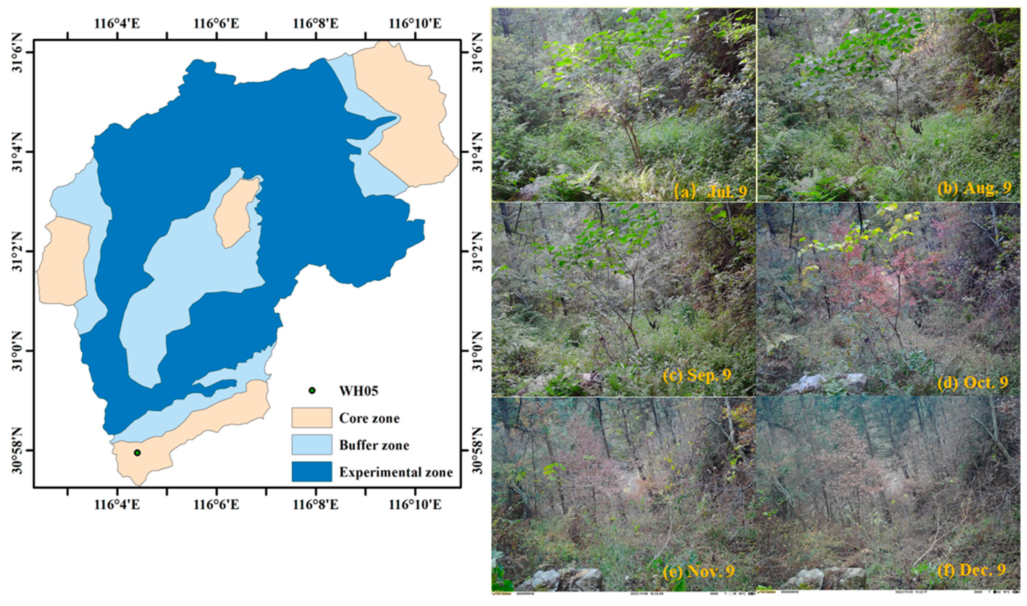
2.1. Study Site
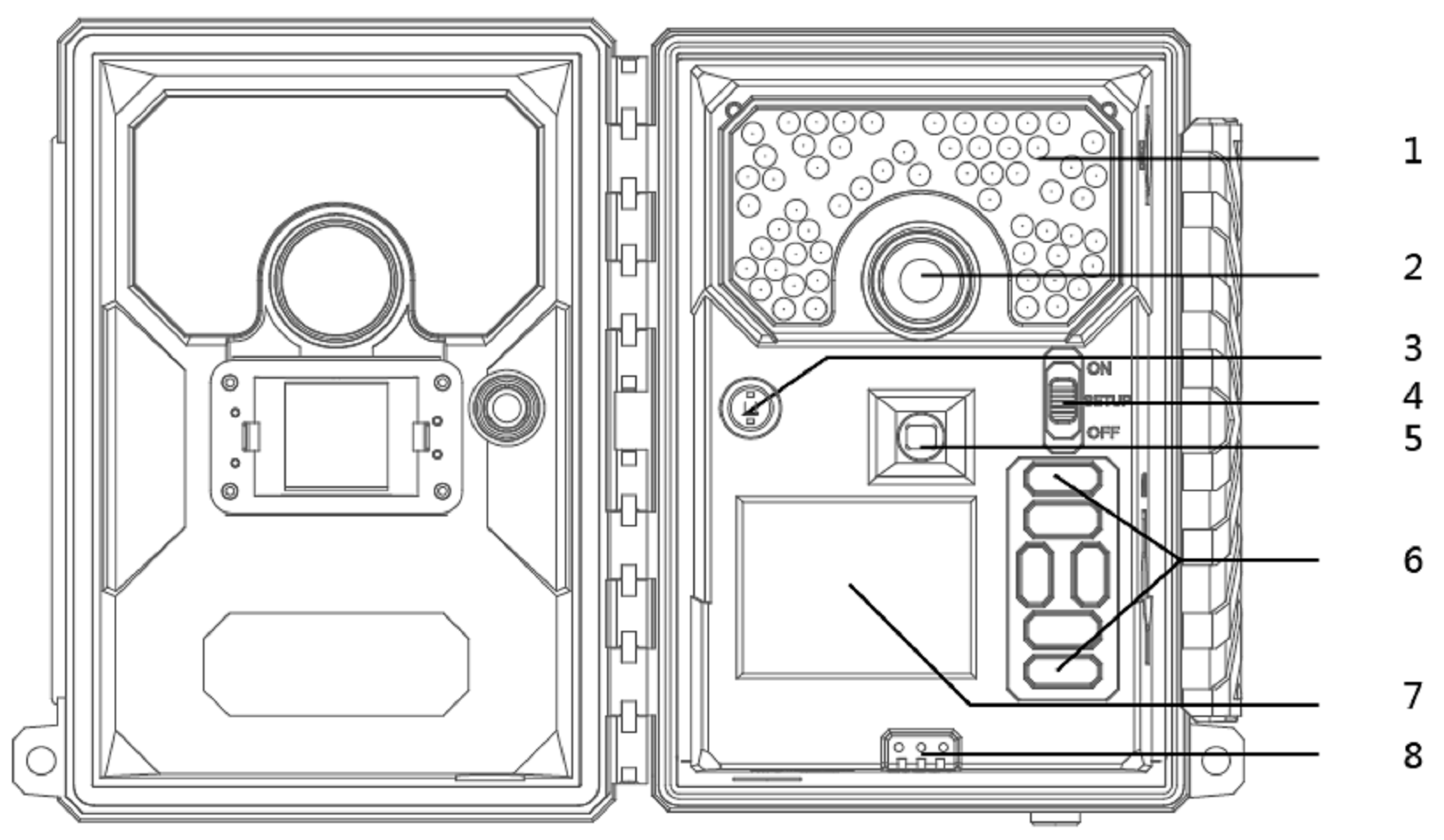
2.2. UVL4-CN IR Camera and Image Preprocessing
2.3. Methods
2.3.1. Vegetation Index
2.3.2. Calculation of the Photoperiod
2.4. Extraction of Autumn Phenology
2.4.1. Process-Based Model
2.4.2. VI Curve Fitted Method
2.4.3. Phenology Extraction Method
3. Results
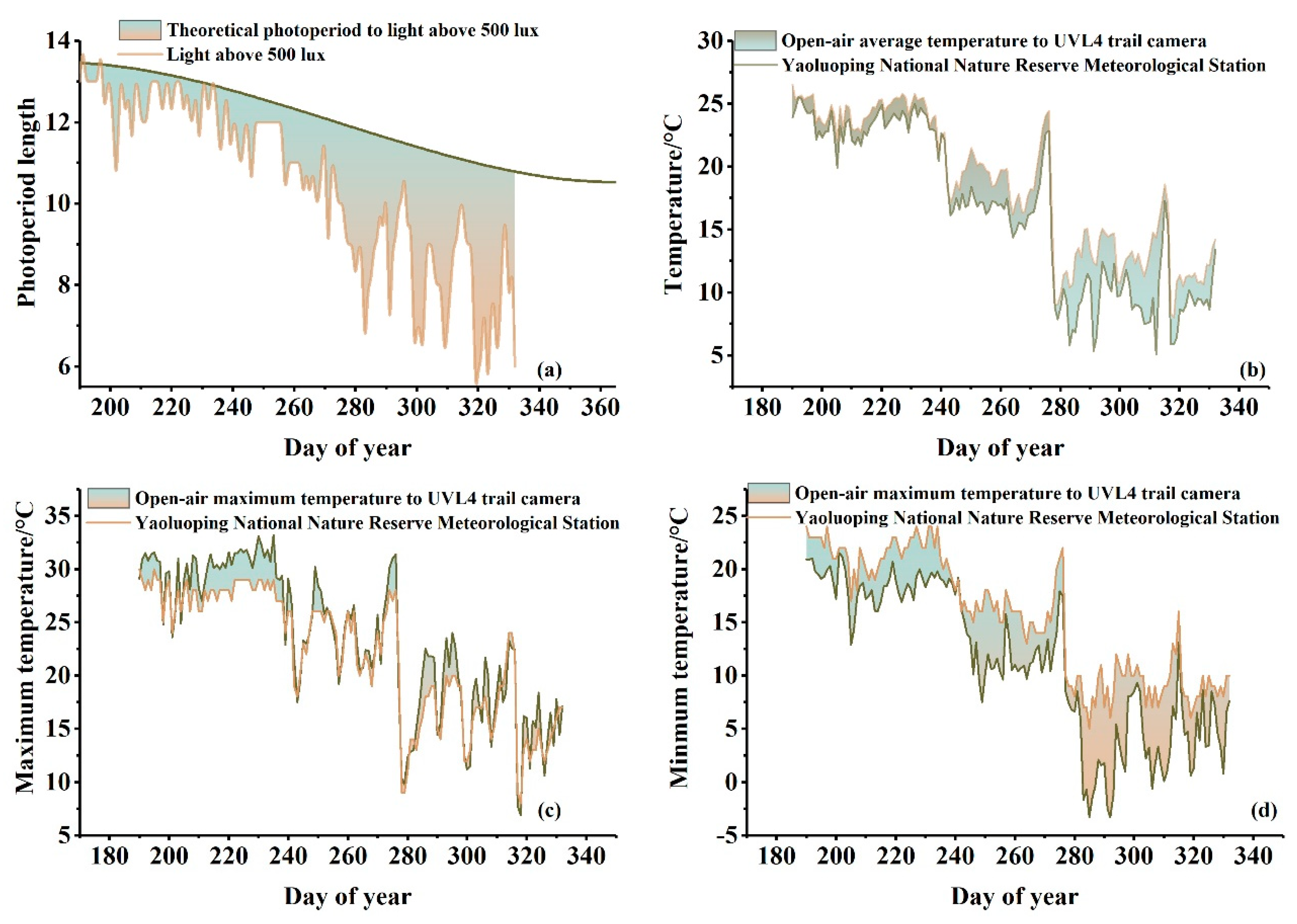
3.1. Temperature and Photoperiod Pattern of Understory Plants
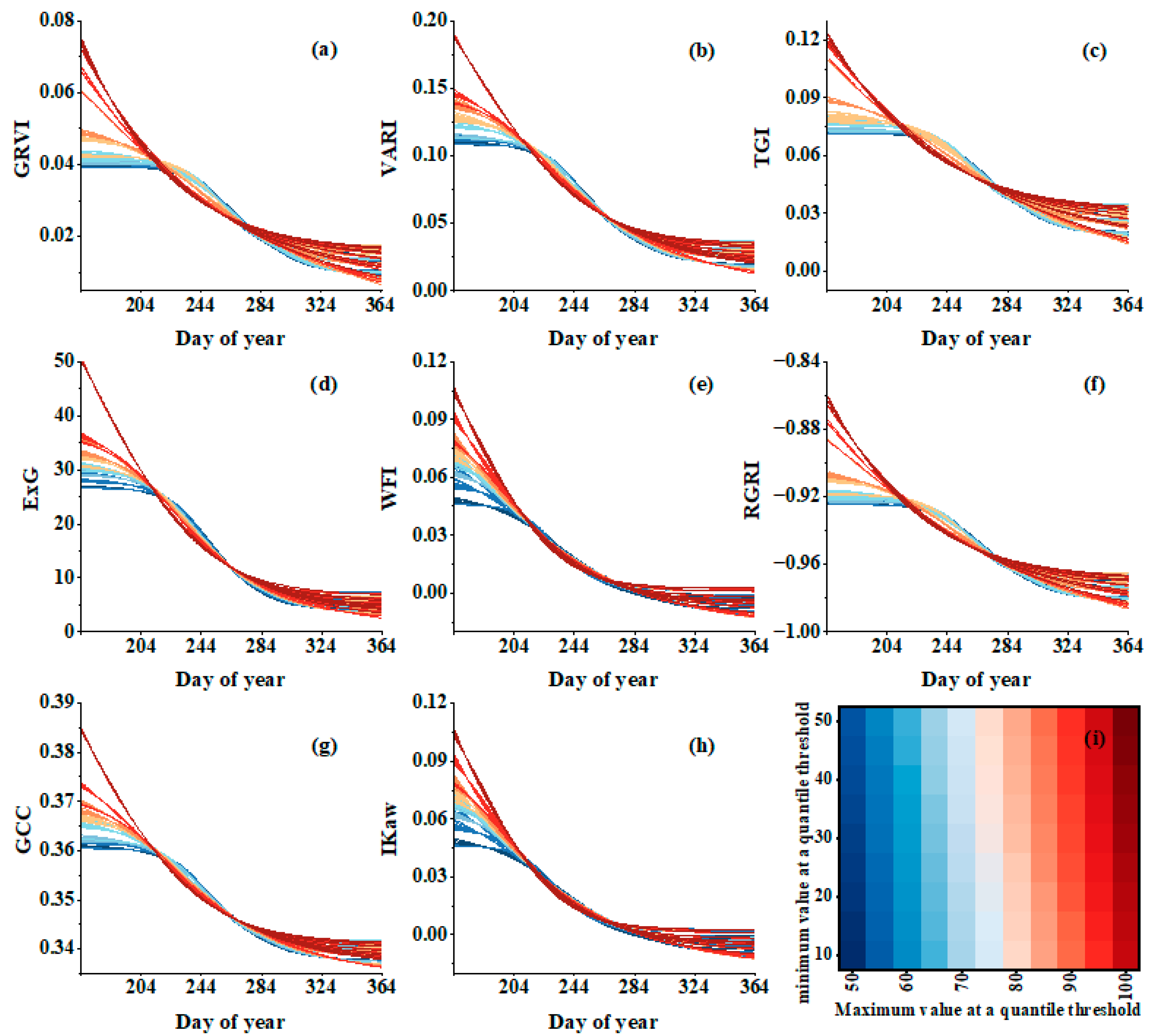
3.2. Comparison in Simulation Greenness Change
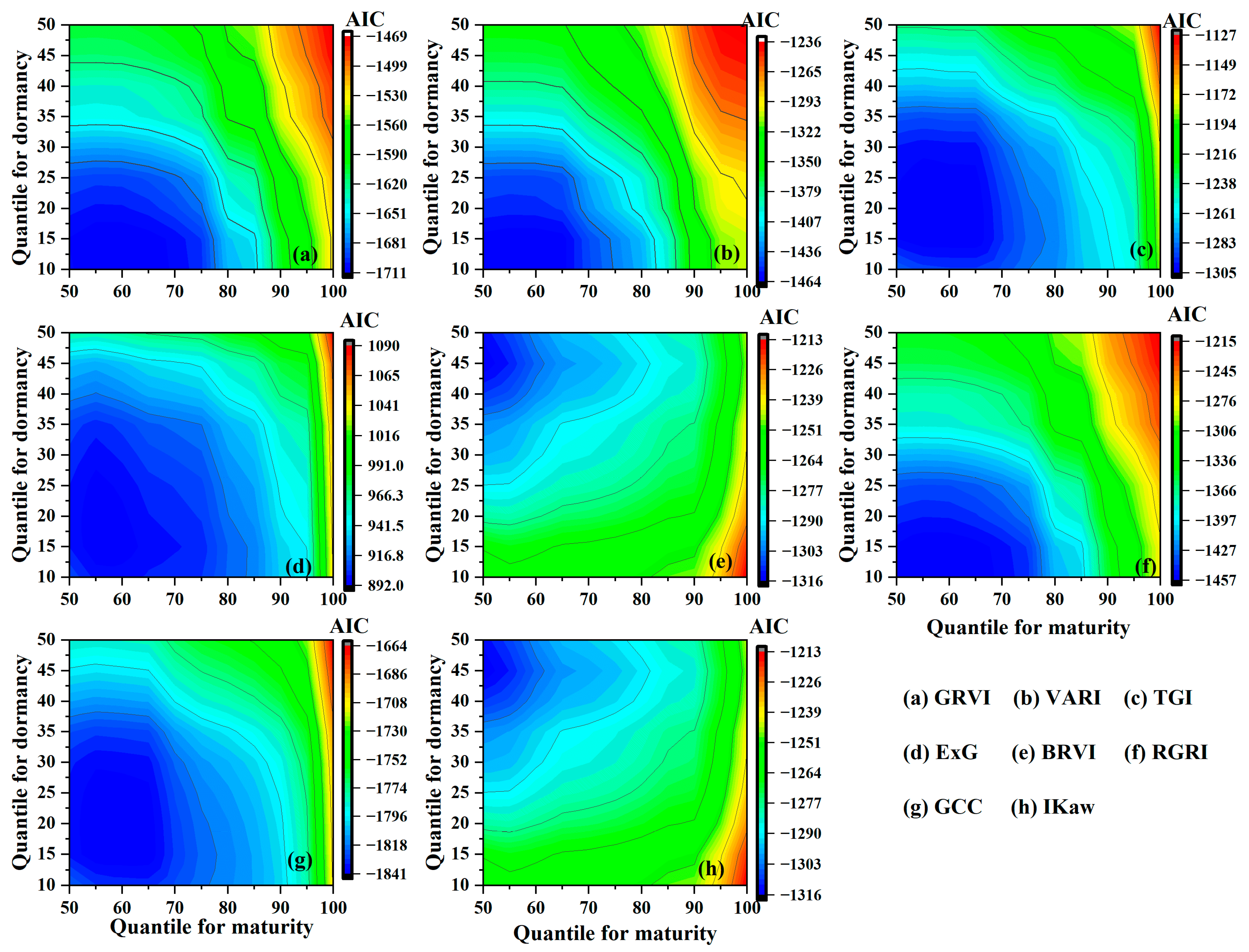
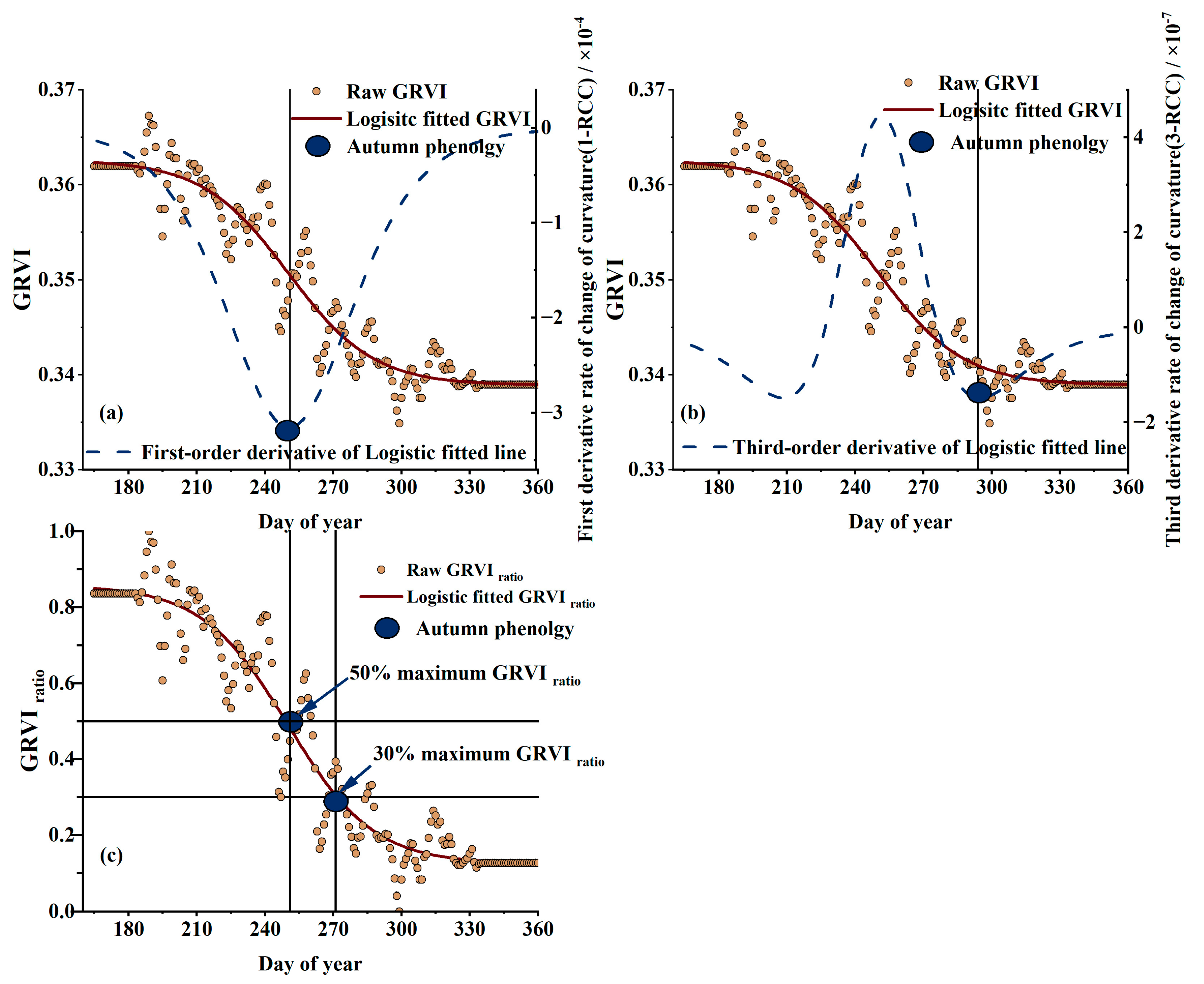
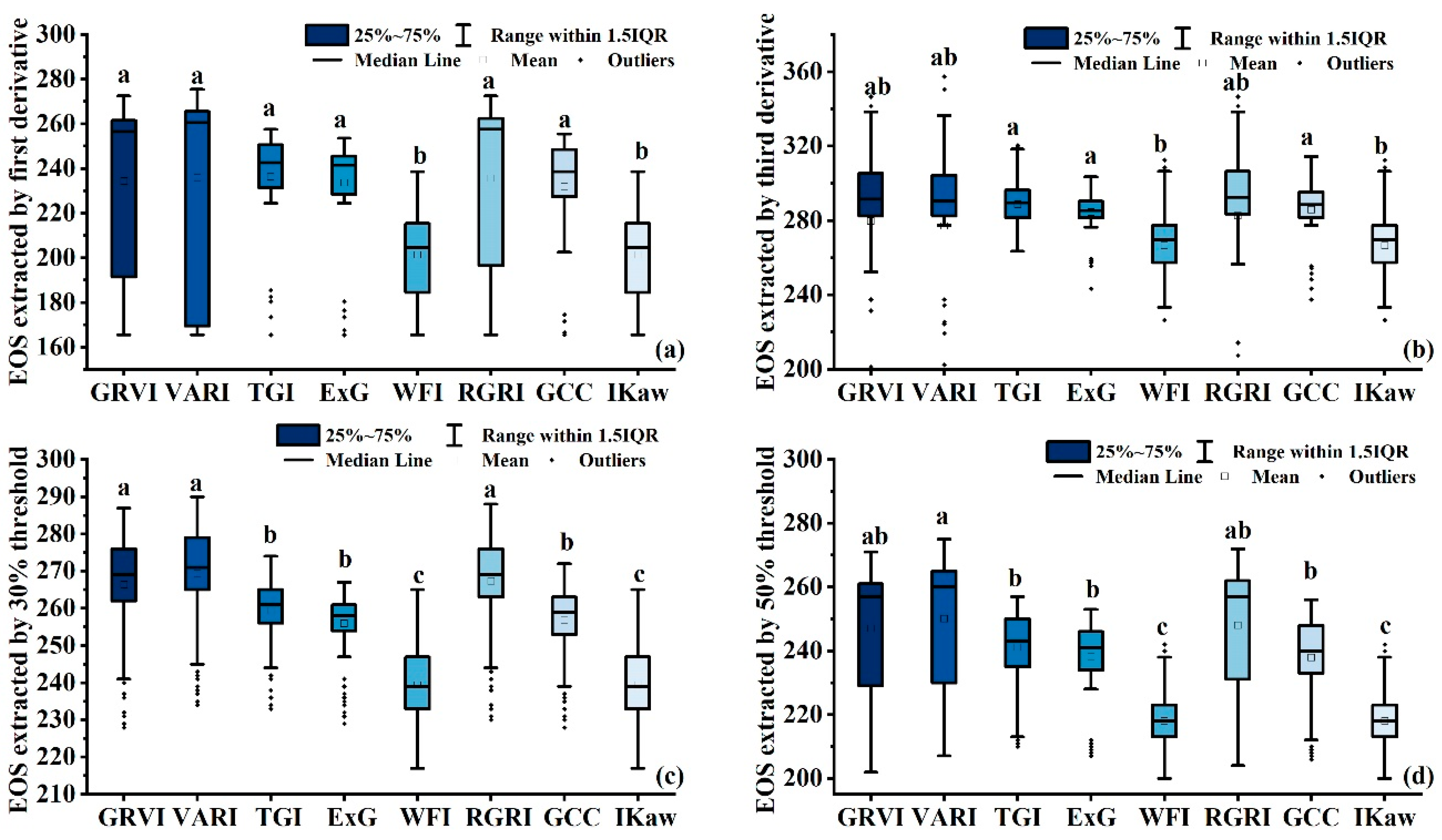
3.3. Comparisons of EOS Derived from VI Time Series
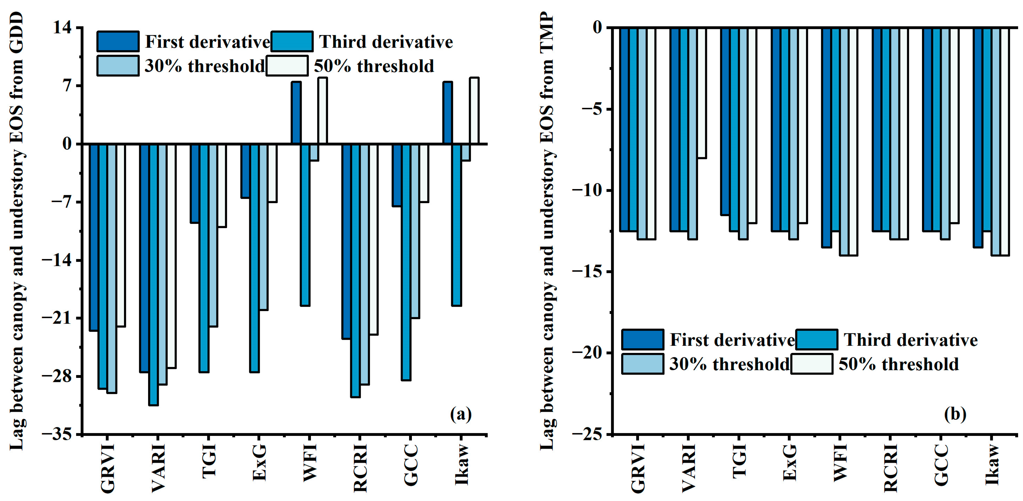
3.4. Tracking EOS from Understory to Overstory Using the CDD Model and TPM
4. Discussion
5. Conclusions
Author Contributions
Funding
Data Availability Statement
Acknowledgments
Conflicts of Interest
Abbreviations
| VI | vegetation index |
| CDD | cold degree days model |
| TPM | temperature and photoperiod multiplicative model |
| NDVI | normalized-difference vegetation index |
| EVI | enhanced vegetation index |
| NIRv | near-infrared of vegetation |
| SOS | start of the growing season |
| EOS | end of the growing season |
| AWB | auto white balance |
| LI | light intensity |
| LD | light direction |
| CCT | correlated color temperature |
| CTR | contrast |
| GL | gray level |
| Sat | saturation |
| Bri | brightness |
| GRVI | green–red vegetation index |
| VARI | visible atmospherically resistant index |
| TGI | triangular greenness index |
| ExG | excess green |
| BRVI | blue–red vegetation index |
| RGRI | red–green ratio index |
| GCC | green chromatic coordinate |
| IKaw | Kawashima index |
Appendix A

| Factor | Abbreviation | Characteristic |
|---|---|---|
| Auto White Balance | AWB | The white balance setting of the image, affecting the accurate reproduction of colors. |
| Light Intensity | LI | The intensity of the light source, affecting the exposure and brightness of the image. |
| Light Direction | LD | The direction of the light source, affecting the shadows and depth of the image. |
| Correlated Color Temperature | CCT | The color temperature of the light source, affecting the warmth or coolness of the image colors. |
| Contrast | CTR | The contrast between light and dark areas in the image, affecting its clarity and detail. |
| Gray Level | GL | The levels of gray in the image, affecting its tonal depth and detail. |
| Saturation | Sat | The purity of the colors in the image, affecting how vivid the colors appear. |
| Brightness | Bri | The overall brightness of the image, affecting its lightness or darkness. |
References
- Fang, J.; Li, X.; Xiao, J.; Yan, X.; Li, B.; Liu, F. Vegetation photosynthetic phenology dataset in northern terrestrial ecosystems. Sci. Data 2023, 10, 300. [Google Scholar] [CrossRef] [PubMed]
- Richardson, A.D.; Keenan, T.F.; Migliavacca, M.; Ryu, Y.; Sonnentag, O.; Toomey, M. Climate change, phenology, and phenological control of vegetation feedbacks to the climate system. Agric. For. Meteorol. 2013, 169, 156–173. [Google Scholar] [CrossRef]
- Wu, C.; Peng, J.; Ciais, P.; Peñuelas, J.; Wang, H.; Beguería, S.; Andrew Black, T.; Jassal, R.S.; Zhang, X.; Yuan, W.; et al. Increased drought effects on the phenology of autumn leaf senescence. Nat. Clim. Change 2022, 12, 943–949. [Google Scholar] [CrossRef]
- Zhang, Y.; Hong, S.; Liu, Q.; Huntingford, C.; Peñuelas, J.; Rossi, S.; Myneni, R.B.; Piao, S. Autumn canopy senescence has slowed down with global warming since the 1980s in the Northern Hemisphere. Commun. Earth Environ. 2023, 4, 173. [Google Scholar] [CrossRef]
- Mestre, L.; Toro-Manríquez, M.; Soler, R.; Huertas-Herrera, A.; Martínez-Pastur, G.; Lencinas, M.V. The influence of canopy-layer composition on understory plant diversity in southern temperate forests. For. Ecosyst. 2017, 4, 6. [Google Scholar] [CrossRef]
- Deng, J.; Fang, S.; Fang, X.; Jin, Y.; Kuang, Y.; Lin, F.; Liu, J.; Ma, J.; Nie, Y.; Ouyang, S.; et al. Forest understory vegetation study: Current status and future trends. For. Res. 2023, 3, 6. [Google Scholar] [CrossRef]
- Donnelly, A.; Yu, R. Temperate deciduous shrub phenology: The overlooked forest layer. Int. J. Biometeorol. 2021, 65, 343–355. [Google Scholar] [CrossRef] [PubMed]
- Saitoh, T.M.; Nagai, S.; Yoshino, J.; Kondo, H.; Tamagawa, I.; Muraoka, H. Effects of canopy phenology on deciduous overstory and evergreen understory carbon budgets in a cool-temperate forest ecosystem under ongoing climate change. Ecol. Res. 2015, 30, 267–277. [Google Scholar] [CrossRef]
- Wu, S.; Wang, J.; Yan, Z.; Song, G.; Chen, Y.; Ma, Q.; Deng, M.; Wu, Y.; Zhao, Y.; Guo, Z.; et al. Monitoring tree-crown scale autumn leaf phenology in a temperate forest with an integration of PlanetScope and drone remote sensing observations. ISPRS J. Photogramm. Remote Sens. 2021, 171, 36–48. [Google Scholar] [CrossRef]
- Piao, S.; Liu, Q.; Chen, A.; Janssens, I.A.; Fu, Y.; Dai, J.; Liu, L.; Lian, X.; Shen, M.; Zhu, X. Plant phenology and global climate change: Current progresses and challenges. Glob. Planet. Change 2019, 25, 1922–1940. [Google Scholar] [CrossRef]
- Wu, C.; Peng, D.; Soudani, K.; Siebicke, L.; Gough, C.M.; Arain, M.A.; Bohrer, G.; Lafleur, P.M.; Peichl, M.; Gonsamo, A.; et al. Land surface phenology derived from normalized difference vegetation index (NDVI) at global FLUXNET sites. Agric. For. Meteorol. 2017, 233, 171–182. [Google Scholar] [CrossRef]
- Peng, D.; Wu, C.; Li, C.; Zhang, X.; Liu, Z.; Ye, H.; Luo, S.; Liu, X.; Hu, Y.; Fang, B. Spring green-up phenology products derived from MODIS NDVI and EVI: Intercomparison, interpretation and validation using National Phenology Network and AmeriFlux observations. Ecol. Indic. 2017, 77, 323–336. [Google Scholar] [CrossRef]
- Zhang, J.; Xiao, J.; Tong, X.; Zhang, J.; Meng, P.; Li, J.; Liu, P.; Yu, P. NIRv and SIF better estimate phenology than NDVI and EVI: Effects of spring and autumn phenology on ecosystem production of planted forests. Agric. For. Meteorol. 2022, 315, 108819. [Google Scholar] [CrossRef]
- Wang, X.; Xiao, J.; Li, X.; Cheng, G.; Ma, M.; Zhu, G.; Altaf Arain, M.; Andrew Black, T.; Jassal, R.S. No trends in spring and autumn phenology during the global warming hiatus. Nat. Commun. 2019, 10, 2389. [Google Scholar] [CrossRef] [PubMed]
- Wu, X.; Niu, C.; Liu, X.; Hu, T.; Feng, Y.; Zhao, Y.; Liu, S.; Liu, Z.; Dai, G.; Zhang, Y.; et al. Canopy structure regulates autumn phenology by mediating the microclimate in temperate forests. Nat. Clim. Change 2024, 14, 1299–1305. [Google Scholar] [CrossRef]
- Moreno-Martínez, Á.; Izquierdo-Verdiguier, E.; Maneta, M.P.; Camps-Valls, G.; Robinson, N.; Muñoz-Marí, J.; Sedano, F.; Clinton, N.; Running, S.W. Multispectral high resolution sensor fusion for smoothing and gap-filling in the cloud. Remote Sens. Environ. 2020, 247, 111901. [Google Scholar] [CrossRef]
- Ye, Y.; Zhang, X.; Shen, Y.; Wang, J.; Crimmins, T.; Scheifinger, H. An optimal method for validating satellite-derived land surface phenology using in-situ observations from national phenology networks. ISPRS J. Photogramm. Remote Sens. 2022, 194, 74–90. [Google Scholar] [CrossRef]
- Richardson, A.D. Tracking seasonal rhythms of plants in diverse ecosystems with digital camera imagery. New Phytol. 2019, 222, 1742–1750. [Google Scholar] [CrossRef]
- Liu, N.; Garcia, M.; Singh, A.; Clare, J.D.J.; Stenglein, J.L.; Zuckerberg, B.; Kruger, E.L.; Townsend, P.A. Trail camera networks provide insights into satellite-derived phenology for ecological studies. Int. J. Appl. Earth Obs. Geoinf. 2021, 97, 102291. [Google Scholar] [CrossRef]
- Richardson, A.D.; Hufkens, K.; Milliman, T.; Aubrecht, D.M.; Chen, M.; Gray, J.M.; Johnston, M.R.; Keenan, T.F.; Klosterman, S.T.; Kosmala, M.; et al. Tracking vegetation phenology across diverse North American biomes using PhenoCam imagery. Sci. Data 2018, 5, 180028. [Google Scholar] [CrossRef]
- Templ, B.; Koch, E.; Bolmgren, K.; Ungersböck, M.; Paul, A.; Scheifinger, H.; Rutishauser, T.; Busto, M.; Chmielewski, F.-M.; Hájková, L.; et al. Pan European Phenological database (PEP725): A single point of access for European data. Int. J. Biometeorol. 2018, 62, 1109–1113. [Google Scholar] [CrossRef] [PubMed]
- Moore, C.; Brown, T.; Duursma, R.; van Dijk, A.; Culvenor, D.; Evans, B.; Huete, A.; Hutley, L.; Maier, S.; Restrepo-Coupe, N.; et al. Australian vegetation phenology: New insights from satellite remote sensing and digital repeat photography. Biogeosciences Discuss. 2016, 13, 5085–5102. [Google Scholar] [CrossRef]
- Nasahara, K.; Nagai, S. Review: Development of an in situ observation network for terrestrial ecological remote sensing: The Phenological Eyes Network (PEN). Ecol. Res. 2015, 30, 211–223. [Google Scholar] [CrossRef]
- Chianucci, F.; Bajocco, S.; Ferrara, C. Continuous observations of forest canopy structure using low-cost digital camera traps. Agric. For. Meteorol. 2021, 307, 108516. [Google Scholar] [CrossRef]
- Steenweg, R.; Hebblewhite, M.; Kays, R.; Ahumada, J.; Fisher, J.T.; Burton, C.; Townsend, S.E.; Carbone, C.; Rowcliffe, J.M.; Whittington, J.; et al. Scaling-up camera traps: Monitoring the planet’s biodiversity with networks of remote sensors. Front. Ecol. Environ. 2017, 15, 26–34. [Google Scholar] [CrossRef]
- Sonnentag, O.; Hufkens, K.; Teshera-Sterne, C.; Young, A.M.; Friedl, M.; Braswell, B.H.; Milliman, T.; O’Keefe, J.; Richardson, A.D. Digital repeat photography for phenological research in forest ecosystems. Agric. For. Meteorol. 2012, 152, 159–177. [Google Scholar] [CrossRef]
- Sakamoto, T.; Shibayama, M.; Kimura, A.; Takada, E. Assessment of digital camera-derived vegetation indices in quantitative monitoring of seasonal rice growth. ISPRS J. Photogramm. Remote Sens. 2011, 66, 872–882. [Google Scholar] [CrossRef]
- Kattenborn, T.; Wieneke, S.; Montero, D.; Mahecha, M.D.; Richter, R.; Guimarães-Steinicke, C.; Wirth, C.; Ferlian, O.; Feilhauer, H.; Sachsenmaier, L.; et al. Temporal dynamics in vertical leaf angles can confound vegetation indices widely used in Earth observations. Commun. Earth Environ. 2024, 5, 550. [Google Scholar] [CrossRef]
- Ide, R.; Oguma, H. Use of digital cameras for phenological observations. Ecol. Inform. 2010, 5, 339–347. [Google Scholar] [CrossRef]
- Wüller, D.; Gabele, H. The Usage of Digital Cameras as Luminance Meters; SPIE: Paris, France, 2007; Volume 6502. [Google Scholar]
- Ouedraogo, D. Interpretable Machine Learning Model Selection for Breast Cancer Diagnosis Based on K-means Clustering. Appl. Med. Inform. 2021, 43, 91–102. [Google Scholar]
- Shahrimie, M.; Mohd Asaari, M.S.; Mishra, P.; Mertens, S.; Dhondt, S.; Wuyts, N.; Scheunders, P. Close-range hyperspectral image analysis for the early detection of stress responses in individual plants in a high-throughput phenotyping platform. ISPRS J. Photogramm. Remote Sens. 2018, 138, 121–138. [Google Scholar] [CrossRef]
- Zeng, Y.; Hao, D.; Huete, A.; Dechant, B.; Berry, J.; Chen, J.M.; Joiner, J.; Frankenberg, C.; Bond-Lamberty, B.; Ryu, Y.; et al. Optical vegetation indices for monitoring terrestrial ecosystems globally. Nat. Rev. Earth Environ. 2022, 3, 477–493. [Google Scholar] [CrossRef]
- Fawcett, D.; Bennie, J.; Anderson, K. Monitoring spring phenology of individual tree crowns using drone-acquired NDVI data. Remote Sens. Ecol. Conserv. 2021, 7, 227–244. [Google Scholar] [CrossRef]
- Tucker, C.J. Red and photographic infrared linear combinations for monitoring vegetation. Remote Sens. Environ. 1979, 8, 127–150. [Google Scholar] [CrossRef]
- Xie, Y.; Civco, D.L.; Silander, J.A. Species-specific spring and autumn leaf phenology captured by time-lapse digital cameras. Ecosphere 2018, 9, e02089. [Google Scholar] [CrossRef]
- Jelínek, Z.; Balazova, K.; Starý, K.; Chyba, J.; Kumhálová, J. Comparing RGB-based vegetation indices from UAV imageries to estimate hops canopy area. Agron. Res. 2020, 18, 2592–2601. [Google Scholar]
- De Swaef, T.; Maes, W.H.; Aper, J.; Baert, J.; Cougnon, M.; Reheul, D.; Steppe, K.; Roldán-Ruiz, I.; Lootens, P. Applying RGB- and Thermal-Based Vegetation Indices from UAVs for High-Throughput Field Phenotyping of Drought Tolerance in Forage Grasses. Remote Sens. 2021, 13, 147. [Google Scholar] [CrossRef]
- Jiang, J.; Cai, W.; Zheng, H.; Cheng, T.; Tian, Y.; Zhu, Y.; Ehsani, R.; Hu, Y.; Niu, Q.; Gui, L.; et al. Using Digital Cameras on an Unmanned Aerial Vehicle to Derive Optimum Color Vegetation Indices for Leaf Nitrogen Concentration Monitoring in Winter Wheat. Remote Sens. 2019, 11, 2667. [Google Scholar] [CrossRef]
- Gamon, J.A.; Surfus, J.S. Assessing leaf pigment content and activity with a reflectometer. New Phytol. 1999, 143, 105–117. [Google Scholar] [CrossRef]
- Ligr, M.; Ron, C.; Natr, L. Calculation of the photo period length. J. Bioinform. 1995, 11, 133–139. [Google Scholar] [CrossRef]
- Xie, Y.; Wang, X.; Wilson, A.M.; Silander, J.A. Predicting autumn phenology: How deciduous tree species respond to weather stressors. Agric. For. Meteorol. 2018, 250–251, 127–137. [Google Scholar] [CrossRef]
- Lang, W.; Chen, X.; Qian, S.; Liu, G.; Piao, S. A new process-based model for predicting autumn phenology: How is leaf senescence controlled by photoperiod and temperature coupling? Agric. For. Meteorol. 2019, 268, 124–135. [Google Scholar] [CrossRef]
- Cesaraccio, C.; Spano, D.; Duce, P.; Snyder, R.L. An improved model for determining degree-day values from daily temperature data. Int. J. Biometeorol. 2001, 45, 161–169. [Google Scholar] [CrossRef] [PubMed]
- Laskin, D.N.; McDermid, G.J.; Nielsen, S.E.; Marshall, S.J.; Roberts, D.R.; Montaghi, A. Advances in phenology are conserved across scale in present and future climates. Nat. Clim. Change 2019, 9, 419–425. [Google Scholar] [CrossRef]
- Ke, M.; Wang, W.; Zhou, Q.; Wang, Y.; Liu, Y.; Yu, Y.; Chen, Y.; Peng, Z.; Mo, Q. Response of leaf functional traits to precipitation change: A case study from tropical woody tree. Glob. Ecol. Conserv. 2022, 37, e02152. [Google Scholar] [CrossRef]
- Yuan, H.; Yan, J.; Liu, Y.; Peng, J.; Wang, X. Influence of vegetation phenological carryover effects on plant autumn phenology under climate change. Agric. For. Meteorol. 2024, 359, 110284. [Google Scholar] [CrossRef]
- van Leeuwen, W.J.D.; Huete, A.R.; Laing, T.W. MODIS Vegetation Index Compositing Approach: A Prototype with AVHRR Data. Remote Sens. Environ. 1999, 69, 264–280. [Google Scholar] [CrossRef]
- Goward, S.N.; Markham, B.; Dye, D.G.; Dulaney, W.; Yang, J. Normalized difference vegetation index measurements from the advanced very high resolution radiometer. Remote Sens. Environ. 1991, 35, 257–277. [Google Scholar] [CrossRef]
- Zeng, L.; Wardlow, B.D.; Xiang, D.; Hu, S.; Li, D. A review of vegetation phenological metrics extraction using time-series, multispectral satellite data. Remote Sens. Environ. 2020, 237, 111511. [Google Scholar] [CrossRef]
- Panwar, A.; Migliavacca, M.; Nelson, J.A.; Cortés, J.; Bastos, A.; Forkel, M.; Winkler, A.J. Methodological challenges and new perspectives of shifting vegetation phenology in eddy covariance data. Sci. Rep. 2023, 13, 13885. [Google Scholar] [CrossRef]
- Nijland, W.; de Jong, R.; de Jong, S.M.; Wulder, M.A.; Bater, C.W.; Coops, N.C. Monitoring plant condition and phenology using infrared sensitive consumer grade digital cameras. Agric. For. Meteorol. 2014, 184, 98–106. [Google Scholar] [CrossRef]
- Reid, A.M.; Chapman, W.K.; Prescott, C.E.; Nijland, W. Using excess greenness and green chromatic coordinate colour indices from aerial images to assess lodgepole pine vigour, mortality and disease occurrence. For. Ecol. Manag. 2016, 374, 146–153. [Google Scholar] [CrossRef]
- Woebbecke, D.M.; Meyer, G.E.; Bargen, K.V.; Mortensen, D.A. Color indices for weed identification under various soil, residue, and lighting conditions. Trans. ASAE 1994, 38, 259–269. [Google Scholar] [CrossRef]
- Zahnd, C.; Arend, M.; Kahmen, A.; Hoch, G. Microclimatic gradients cause phenological variations within temperate tree canopies in autumn but not in spring. Agric. For. Meteorol. 2023, 331, 109340. [Google Scholar] [CrossRef]
- Gressler, E.; Jochner, S.; Capdevielle-Vargas, R.M.; Morellato, L.P.C.; Menzel, A. Vertical variation in autumn leaf phenology of Fagus sylvatica L. in southern Germany. Agric. For. Meteorol. 2015, 201, 176–186. [Google Scholar] [CrossRef]
- Kikuzawa, K.; Lechowicz, M.J. Ecosystem Perspectives on Leaf Longevity. In Ecology of Leaf Longevity; Springer Tokyo: Tokyo, Japan, 2011; pp. 109–119. [Google Scholar]
- Ismaeel, A.; Tai, A.P.K.; Santos, E.G.; Maraia, H.; Aalto, I.; Altman, J.; Doležal, J.; Lembrechts, J.J.; Camargo, J.L.; Aalto, J.; et al. Patterns of tropical forest understory temperatures. Nat. Commun. 2024, 15, 549. [Google Scholar] [CrossRef]


| VI | Abbrev. | Formula | Characteristic | Reference |
|---|---|---|---|---|
| Green–red vegetation index | GRVI | Sensitive to land cover types | [35] | |
| Visible atmospherically resistant index | VARI | Anthocyanin in plant leaves | [36] | |
| Triangular greenness index | TGI | Plant health and stress | [37] | |
| Excess green | ExG | Plant greenness | [37] | |
| Blue–red vegetation index | BRVI | Plant health and chlorophyll | [38] | |
| Red–green ratio index | RGRI | Vegetation health and vitality | [39] | |
| Green chromatic coordinate | GCC | Vegetation dynamic | [18] | |
| Kawashima index | IKaw | Leaf nitrogen concentration | [40] |
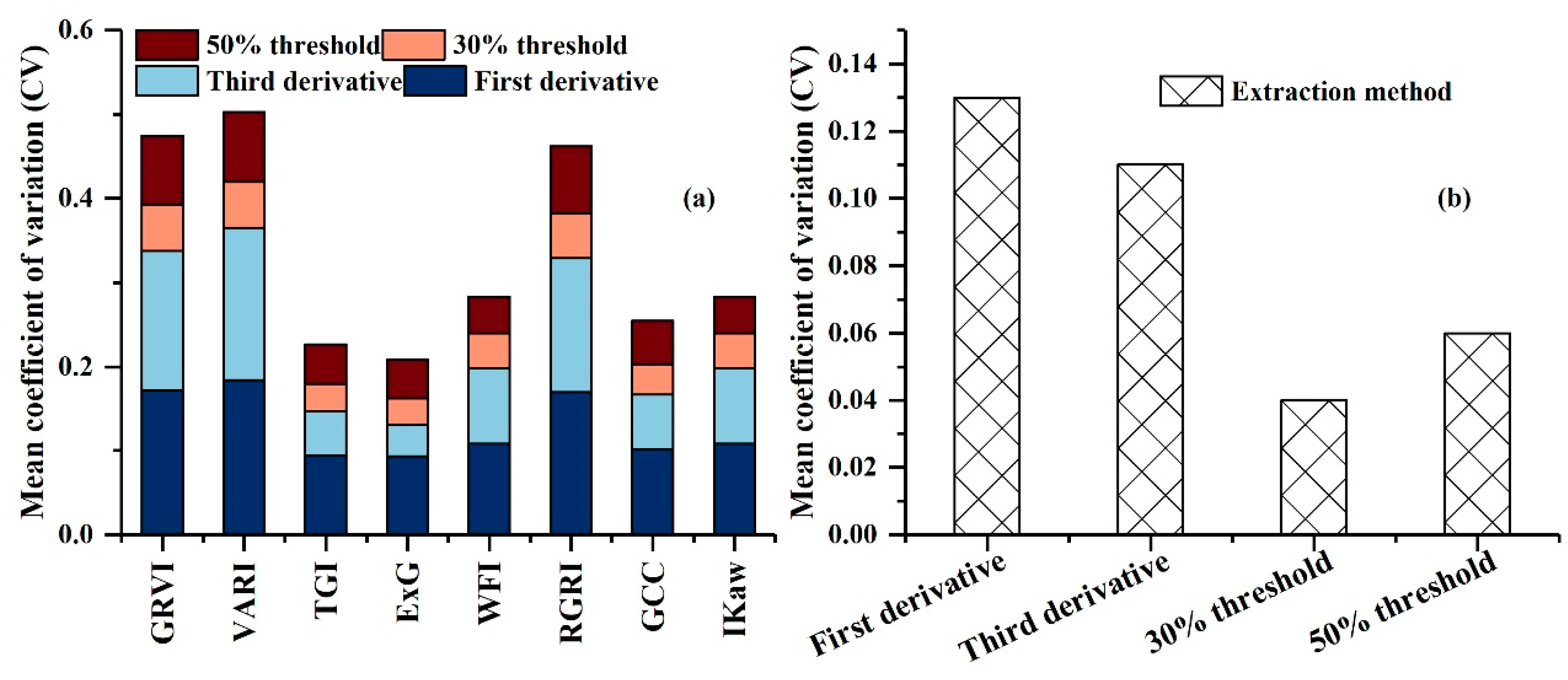
| VI | First Derivative | Third Derivative | 30% Threshold | 50% Threshold |
|---|---|---|---|---|
| GRVI | 268.5 | 312.5 | 284 | 268 |
| VARI | 273.5 | 314.5 | 288 | 273 |
| TGI | 252.5 | 291.5 | 267 | 253 |
| ExG | 249.5 | 289.5 | 264 | 250 |
| WFI | 233.5 | 262.5 | 244 | 233 |
| RCRI | 269.5 | 313.5 | 285 | 269 |
| GCC | 250.5 | 293.5 | 266 | 250 |
| Ikaw | 233.5 | 262.5 | 244 | 233 |
Disclaimer/Publisher’s Note: The statements, opinions and data contained in all publications are solely those of the individual author(s) and contributor(s) and not of MDPI and/or the editor(s). MDPI and/or the editor(s) disclaim responsibility for any injury to people or property resulting from any ideas, methods, instructions or products referred to in the content. |
© 2025 by the authors. Licensee MDPI, Basel, Switzerland. This article is an open access article distributed under the terms and conditions of the Creative Commons Attribution (CC BY) license (https://creativecommons.org/licenses/by/4.0/).
Share and Cite
Yuan, H.; Zhang, J.; Zhang, H.; Xu, W.; Peng, J.; Wang, X.; Chen, P.; Li, P.; Lu, F.; Yan, J.; et al. Monitoring Autumn Phenology in Understory Plants with a Fine-Resolution Camera. Remote Sens. 2025, 17, 1025. https://doi.org/10.3390/rs17061025
Yuan H, Zhang J, Zhang H, Xu W, Peng J, Wang X, Chen P, Li P, Lu F, Yan J, et al. Monitoring Autumn Phenology in Understory Plants with a Fine-Resolution Camera. Remote Sensing. 2025; 17(6):1025. https://doi.org/10.3390/rs17061025
Chicago/Turabian StyleYuan, Huanhuan, Jianliang Zhang, Haonan Zhang, Wanggu Xu, Jie Peng, Xiaoyue Wang, Peng Chen, Pinghao Li, Fei Lu, Jiabao Yan, and et al. 2025. "Monitoring Autumn Phenology in Understory Plants with a Fine-Resolution Camera" Remote Sensing 17, no. 6: 1025. https://doi.org/10.3390/rs17061025
APA StyleYuan, H., Zhang, J., Zhang, H., Xu, W., Peng, J., Wang, X., Chen, P., Li, P., Lu, F., Yan, J., & Wang, Z. (2025). Monitoring Autumn Phenology in Understory Plants with a Fine-Resolution Camera. Remote Sensing, 17(6), 1025. https://doi.org/10.3390/rs17061025