Article

Unsupervised Rural Flood Mapping from Bi-Temporal Sentinel-1 Images Using an Improved Wavelet-Fusion Flood-Change Index (IWFCI) and an Uncertainty-Sensitive Markov Random Field (USMRF) Model

1
Department of Photogrammetry and Remote Sensing, K. N. Toosi University of Technology, Tehran 19697-64499, Iran
2
Department of Technology and Society, Faculty of Engineering, Lund University, P.O. Box 118, SE-221 00 Lund, Sweden
*
Author to whom correspondence should be addressed.
Remote Sens. 2025, 17(6), 1024; https://doi.org/10.3390/rs17061024
Submission received: 30 January 2025 / Revised: 10 March 2025 / Accepted: 11 March 2025 / Published: 14 March 2025

Abstract

:
Synthetic aperture radar (SAR) remote sensing (RS) technology is an ideal tool to map flooded areas on account of its all-time, all-weather imaging capability. Existing SAR data-based change detection approaches lack well-discriminant change indices for reliable floodwater mapping. To resolve this issue, an unsupervised change detection approach, made up of two main steps, is proposed for detecting floodwaters from bi-temporal SAR data. In the first step, an improved wavelet-fusion flood-change index (IWFCI) is proposed. The IWFCI modifies the mean-ratio change index (CI) to fuse it with the log-ratio CI using the discrete wavelet transform (DWT). The IWFCI also employs a discriminant feature derived from the co-flood image to enhance the separability between the non-flood and flood areas. In the second step, an uncertainty-sensitive Markov random field (USMRF) model is proposed to diminish the over-smoothness issue in the areas with high uncertainty based on a new Gaussian uncertainty term. To appraise the efficacy of the floodwater detection approach proposed in this study, comparative experiments were conducted in two stages on four datasets, each including a normalized difference water index (NDWI) and pre-and co-flood Sentinel-1 data. In the first stage, the proposed IWFCI was compared to a number of state-of-the-art (SOTA) CIs, and the second stage compared USMRF to the SOTA change detection algorithms. From the experimental results in the first stage, the proposed IWFCI, yielding an average F-score of 86.20%, performed better than SOTA CIs. Likewise, according to the experimental results obtained in the second stage, the USMRF model with an average F-score of 89.27% outperformed the comparative methods in classifying non-flood and flood classes. Accordingly, the proposed floodwater detection approach, combining IWFCI and USMRF, can serve as a reliable tool for detecting flooded areas in SAR data.

Graphical Abstract

1. Introduction

Floods are catastrophic natural disasters that cause substantial damage to ecosystems, infrastructures, economies, and agricultural areas all over the world [1,2,3,4,5]. Mapping flood extent is necessary for relief operations, disaster management, and damage mitigation and assessment [6,7]. In this context, satellite-based remote sensing (RS) provides a repetitive view and vast spatial coverage over the earth’s surface, enabling continuous monitoring of flooded areas [8,9]. In recent years, optical and synthetic aperture radar (SAR) RS data have increasingly been used for flood mapping. Despite the high interpretability of the optical data, these sensors cannot collect data in cloudy weather [10], which is typical during floods [11]. In contrast, SAR satellites, supporting all-time, all-weather data acquisition, are appropriate for flood monitoring over large areas [12].
Since the floodwater results in a low return due to the specular scattering, floods in rural areas appear dark in SAR images [13]. This principle has led to the development of numerous SAR-based floodwater detection approaches that could be divided into five categories, including supervised classification [14], thresholding [15], change detection (CD) [16], segmentation [17], and deep learning [18]. Among these methods, CD algorithms can diminish misdetections to a large degree in water-like areas, such as shadows, by comparing SAR images captured before and during floods over the same geographical extent [6,19].
Change detection methods based on RS data can be generally categorized into supervised and unsupervised approaches [16,20]. Supervised CD methods are often costly and time-consuming as they rely on training samples (labeled data) for the classification task [21]. In contrast, due to no demand for training samples, unsupervised CD (UCD) techniques are independent of prior knowledge of the flooded area, allowing for near real-time automatic extraction of the flood pixels [22,23,24]. UCD approaches used for floodwater mapping generally consist of three major steps: (1) preprocessing, (2) change index (CI) formation, and (3) classifying CI into unchanged (non-flood) and changed (flood) categories [25]. In more detail, the first step intends to geometrically and radiometrically correct bi-temporal SAR data. In the second step, pre- and co-flood SAR data are compared through mathematical operators to form a feature accentuating the changed (flooded) regions. In the literature, two types of CIs, including (1) individual and (2) fused SAR CIs, have been frequently used to highlight inundated areas from SAR data. Conventional individual SAR CIs used in the flood application involve difference [26,27,28], normalized difference [23,29,30,31], ratio [32], and log-ratio [6,33,34]. However, each individual CI has some particular limitations in reflecting the flood changes. In more detail, the difference-based CIs depend on both relative backscatter changes and the backscatter values in the pre-flood (reference) SAR image [34]. Therefore, flood change patterns in these CIs vary over low- and high-backscatter areas, possibly resulting in either flood information loss or noisy changes [34,35]. Conversely, the ratio CI mostly relies on the relative backscatter changes, exhibiting similar change patterns for low- and high-backscatter pixels; however, it suffers from the speckle noise, which is an inherent issue in SAR images. The log-ratio CI is an improved variant of the ratio CI, where a logarithm operator is used to enhance low-intensity changes while suppressing the speckle noise by compressing the change variation range in the ratio image [36]. Nevertheless, this compression also weakens some high-intensity changes [37] and may reduce the contrast between the non-flood and flood classes. Lately, fused CIs have been devised to diminish the limitations of the individual CIs by integrating their complementary change information, thus raising the contrast between the non-flood and flood areas [38]. Gong et al. [37] and Moghimi et al. [39] integrated the log-ratio and mean-ratio CIs using the discrete wavelet transform (DWT) image fusion technique. The fused CI reflected changed pixels properly while restraining the background (unchanged) area. Hou et al. [40] also used the DWT algorithm to combine the Gauss log-ratio with log-ratio to increase the distinction between changed and unchanged areas.
In the third step of the UCD methods, the CI is partitioned into unchanged (non-flood) and changed (flood) classes. To perform this binary segmentation, clustering [41,42], thresholding [22,43], and Markov random fields (MRFs)-based approaches have been frequently used in previous studies. Both the clustering and thresholding approaches ignore integrating the change intensity information with the spatial context (adjacent labels), resulting in noisy change (flood) maps [44]. On the other hand, as the statistical models that carry this integration out, MRFs have frequently been used in the RS data-based UCD literature to segment the CIs [23,44,45,46,47,48,49,50]. However, the neighborhood spatial context (smoothness) used in the traditional MRF model is fixed for all the pixels throughout the flood CI. This limitation can cause the over-smoothness (over-prediction) issue to the flood pixels in the inter-class area referring to the region around the boundary between non-flood and flood classes, also regarded as the uncertainty area. A limited number of studies have tackled the MRF over-smoothness issue in these areas. Gu et al. [51] considered an uncertainty region in the inter-class area based on the fuzzy membership degrees derived from the fuzzy c-means (FCM) algorithm to decrease the over-smoothness issue in the uncertainty region. Likewise, He et al. [52] also used the fuzzy membership degrees derived from FCM to designate a local uncertainty term and incorporate it into the MRF model to diminish the over-predictions in the uncertain area.
Despite noteworthy achievements in the preceding SAR CD-based rural floodwater mapping studies, they face some shortcomings that should be addressed properly. In detail, on the one hand, previous methods mostly use generic individual CIs, including but not limited to the ratio, log-ratio, and normalized difference-based CIs. As mentioned before, due to either low inter-class contrast or many change artifacts, these CIs may result in unsatisfactory flood extent maps. On the other hand, a remarkable gap in the fused CIs introduced in [37,40] is ignoring the co-flood image in the fusion process. This can lead to a low separability between the non-flood and flood classes. As the non-flood land covers have a bright appearance in SAR images while the flooded rural areas appear in a dark tone, incorporating the flood image in the fusion process can enhance the inter-class contrast and the accuracy of recognizing flooded areas. Additionally, despite well-reflecting the high-intensity changes, the mean-ratio CI in [37] has a noisy background, which leads to substantial artifacts in the fused CI. Indeed, an efficient flood change index with minimum background artifacts and high separability between flooded and non-flooded areas is still a gap in SAR CD-based floodwater detection. Regarding the MRF models previously refined for uncertainty areas, the modifications have considerably restrained the model to the initialization algorithm, i.e., the FCM clustering algorithm. Hence, this degrades the smoothness of the MRF model even over the flood pixels with low uncertainties, which may result in flood maps missing some inundated pixels inside the flood objects.
To tackle the aforementioned challenges, the present study proposes a novel unsupervised floodwater detection method. Since it operates in an unsupervised manner and is independent from the prior information about the area, the proposed approach is highly automated and adaptable to near real-time SAR data-based mapping of flooded rural areas in all-time, all-weather conditions. In the proposed method, a new uncertainty-sensitive MRF (USMRF) model is applied to a novel improved wavelet-fusion flood-change index (IWFCI). The proposed IWFCI employs a discriminant feature derived from the co-flood image to raise the contrast between flooded and non-flooded areas. Furthermore, an adaptive weighting scheme is used in the fused CI to minimize noise and artifacts. These enable the proposed IWFCI to provide more accurate flood change information in rural areas compared to the traditional individual and fused CIs. As for the proposed USMRF model, it optimally combines the flood change intensity information with the spatial context to diminish excessive smoothness (overestimations) in uncertain regions. In this way, the synergy of the IWFCI and USMRF, shaping the proposed SAR data-based floodwater mapping approach, can offer precise floodwater extent maps. To sum up, the key contributions of the present research are listed as follows:
  • A novel fused flood-CI, namely IWFCI, is introduced in this study, where the mean-ratio CI is modified and then integrated with the log-ratio CI and flood image to accurately reflect the flood-related changes in rural areas.
  • A Gaussian-like uncertainty penalty term based on the gray values of the CI is constructed and incorporated into the MRF to decrease the errors of the model over inter-class uncertain areas.
The rest of the present study is structured as follows: Section 2 details the proposed rural flood mapping approach, study areas, and datasets considered in this work. In Section 3, the experimental results achieved for four datasets are presented and discussed. Finally, Section 4 concludes the study.

2. Materials and Methods

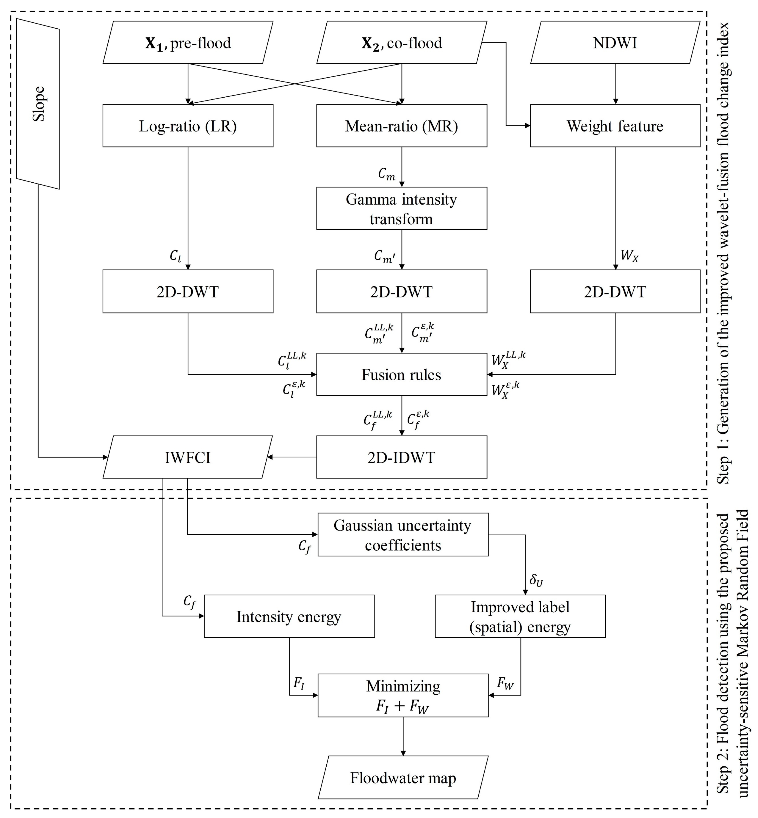
2.1. Proposed Unsupervised Floodwater Detection Approach

Suppose X 1 = x 1 i , j | 1 i a , 1 j b and X 2 = x 2 i , j | 1 i a , 1 j b represent bi-temporal geometrically and radiometrically corrected SAR images of size a × b in linear scale, captured over the same geographical area at times t 1 and t 2 , respectively. The present study mainly pursues two objectives: (1) constructing a reliable fused flood change index C f = c f i , j | 1 i a , 1 j b and (2) improving the performance of a statistical model in highly uncertain areas. Corresponding to these aims, the proposed floodwater detection approach consists of two main steps, as depicted in Figure 1. In the first step, to form an improved wavelet-fusion flood-change index (IWFCI), the mean-ratio CI is modified and combined with the log-ratio CI and a feature derived from the flood image. In the second step, IWFCI is classified by an uncertainty-sensitive MRF (USMRF) model improved in high-uncertain areas to generate a flood map. M F = m f i , j | 1 i a , 1 j b where m f i , j = 0 and m f i , j = 1 denotes the non-flood and flood pixels, respectively.

2.1.1. Improved Wavelet-Fusion Flood Change Index

Fused change indices, due to combining two individual CIs, can provide complementary change information and enhance the inter-class contrast, i.e., the contrast between change and no-change classes [38]. In [37], the wavelet-fusion change index (WFCI) was introduced, where individual CIs were integrated using the 2-dimensional discrete wavelet transform (2D-DWT) fusion technique. As a simple and computationally efficient algorithm, 2D-DWT is a multiresolution fusion algorithm that maintains image details while reducing noise during the fusion [37,53].
In general, the WFCI is generated in four steps. In the first step, the log-ratio (LR) and mean-ratio (MR) [54] CIs were computed as follows:
C m = n 1 m i n μ X 1 m i n X μ X 1 , μ X 2 , m i n X μ X 1 , μ X 2 μ X 1
C l = n l o g X 1 m i n X X 1 , X 2  
where μ X 1 and μ X 2 in C m are the local mean values of the pre-and co-flood SAR images, m i n [ . ] is an operator computing the minimum mean-ratio value, and m i n X [ . ] takes the minimum value between pre- and co-flood times as floodwaters in rural areas appear dark in X 2 . Also, n [.] maps the CIs between 0 and 1 based on the ‘min–max’ normalization. As mentioned previously, the logarithm operator in LR enhances low-intensity changes while suppressing the adverse impact of the speckle noise. However, this can weaken high-intensity changes and reduce the inter-class contrast in LR. On the other hand, although MR is superior in reflecting the changes, it has a rough background, probably owing to the amplification of the changes corresponding to the low-amplitude pixels of the bi-temporal.
In the second step, the 2D-DWT algorithm uses low- and high-pass filtering to decompose the individual CIs ( C u , u : l , m ) at each k level of decomposition ( k = 1,2 , , K ) into four sub-bands. The decomposed sub-bands include one low-frequency (approximation) sub-band ( C u L L , k ) and three high-frequency (detailed) sub-bands: horizontal ( C u L H , k ), vertical ( C u H L , k ), and diagonal ( C u H H , k ) sub-bands. The C u L L , k captures the primary characteristics of C u , while C u L H , k , C u H L , k , and C u H H , k   represent details in C u . In the second step, corresponding sub-bands are then fused using two types of fusion rules: (1) averaging the approximation sub-bands (Equations (2) and (3)) minimum local area energy selection for the detailed sub-bands (Equation (4)).
C f L L , k i , j = C l L L , k i , j + C m L L , k i , j 2
C f ε , k i , j = C m ε , k i , j ,     E m ε , k i , j < E l ε , k i , j C l ε , k i , j ,     E m ε , k i , j E l ε , k i , j ;   ε : L H , H L , H H
where l , m , and f indicate the LR, MR, and fused CIs, respectively, and E ε , k specifies the local area energy coefficient at level k , computed as follows:
E u ε , k i , j = p ϵ N i , j C u ε , k p 2 ;   u : l , m
where N i , j signifies the local window centered at ( i , j ) , involving C u ε , k p . Lastly, the 2-dimensional inverse DWT (2D IDWT) is applied on the fused sub-bands, i.e., C f L L , k and C f ε , k ( ε : L H , H L , H H ) to reach the fused index C f .
As mentioned earlier, the WFCI has two shortcomings in reflecting changed (flooded) areas. Firstly, the MR CI contains many noisy changes and artifacts in its background, causing the fused index to suffer from noisy changes as well. Secondly, WFCI does not use co-flood image information during the fusion, while the co-flood image is a beneficial source with high contrast between flood and non-flood classes.
In order to address the aforementioned limitations, two modifications were made to the typical WFCI to devise an improved WFCI (IWFCI). In detail, to tackle the first issue, an adaptive weighting scheme was proposed in this study to refine the MR CI before its integration with LR. As stated before, the LR CI enhances the low-intensity changes but suppresses some high-intensity ones due to the logarithm compression. Hence, the high-intensity changes in MR should contribute more than the low-intensity ones to complement LR in the fusion process. Thereby, MR change intensities should be weighted by an intensity transform operator that highly mitigates the noisy low-intensity changes in the background with a minimum impact on the high-intensity changes. This can diminish the adverse impact of MR’s noisy background on the fused CI to a large degree. Due to mapping low intensities into darker ones [55], the Gamma intensity transform with a power value larger than 1 can properly satisfy this condition. Motivated by this, MR was weighted with the Gamma transform as follows:
C m = C m γ
where C m characterizes the modified MR CI, and γ represents the intensity transform parameter (power) in the Gamma transform, which was set to 2.5 based on empirical analyses.
To address the second issue, the flood image was incorporated into the fusion procedure to enhance the inter-class contrast and reduce noise in the fused CI. To do so, a weighting feature based on the flood image was first obtained as follows:
W X = 1 n [ X 2 d B ]
where X 2 d B denotes the flood image in decibel (dB) scale, and n [ . ] is the normalization operator used before. Thereafter, the pixels in W X with positive NDWI were set to 0 to mask permanent waters, and W X was decomposed into the approximation ( W X L L , k ) and detailed sub-bands ( W X ε , k ; ε : L H , H L , H H ). Updating Equations (3) and (4), the decomposition coefficients of LR and the modified MR were next refined by those of W X as below:
C f L L , k i , j = W X L L , k ( i , j ) C l L L , k i , j + C m L L , k i , j 2
C f ε , k i , j = W X ε , k ( i , j ) C m ε , k i , j ,     E m ε , k i , j < E l ε , k i , j W X ε , k ( i , j ) C l ε , k i , j ,     E m ε , k i , j E l ε , k i , j ;   ε : L H , H L , H H
The IWFCI was next produced by applying the 2D IDWT on the new fused sub-bands. Finally, the changes with slopes larger than 5 degrees were also set to 0 in IWFCI to remove spurious flood pixels over flood-unlikely areas [30,56].

2.1.2. Floodwater Detection Using the Uncertainty-Sensitive MRF (USMRF)

Let X = { x d | d = 1 ,   , D } be a set of the D pixels in the proposed IWFCI, and W = { w d | d = 1 ,   , D } be their labels attained by the Otsu thresholding [57]. The MRF model relabels x d by the maximum a posteriori (MAP) theory, expressed as
W * = a r g m a x P W p Y W
where P ( W ) denotes the prior probability of the class of interest, and p Y W characterizes the probability distribution of IWFCI. The MRF theory also states the MAP solution for a pixel of interest ( x d ) is equivalent to minimizing the following total energy term:
F T ( x d ) = F I ( x d ) + F W ( x d )
where F I ( x d ) represents the intensity energy, formulated as
F I ( x d ) = 1 2 ln 2 π σ c 2 + 1 2 x d μ c 2 σ c 2
where μ c and σ c 2 signify the mean and variance of class c , respectively, and F W ( x d ) is also the spatial (label) energy, outlined as below:
F W ( x d ) = β m = 1 M I w d , w m
where β > 0 is the spatial weight parameter regulating the impact of the pixels neighboring x d , and I w d , w m is the Potts model [50,52] defined as
I w d , w m = 0 ,             w d = w m 1 ,             w d w m
where w m ( m = 1 : M ) are the labels of pixels surrounding the x d in the neighborhood Ω d .
Despite the ability of MRF to model spatial context, the model faces an inherent issue arising from using a fixed value of β in the label energy function. This leads to the over-smoothness problem in high-uncertainty areas, resulting in over-predictions. High uncertainty typically occurs near boundaries between the flood and non-flood classes, where the pixels of the two classes are close in gray value. Accordingly, an uncertainty-sensitive penalty function was proposed in this study to tackle this limitation. In the proposed approach, uncertainty coefficients ( δ U m ) for the pixels in Ω d were first calculated as follows:
δ U m x m = 1 + e x p x m μ ¯ / 2 σ μ ¯ 2 ;   m = 1 : M
where μ ¯ is the average of the mean values (centers) of the flood ( μ f ) and non-flood ( μ n f ) classes, and σ μ ¯ denotes the standard deviation of the IWFCI ( C f ) around μ ¯ , estimated as
σ μ ¯ = x d μ ¯ 2 / D ;       d = 1 , , D
Afterward, the average uncertainty coefficient ( δ ¯ U ) for each neighborhood Ω d was estimated as follows:
δ ¯ U x m = R / M A v g Ω d δ U m x m ;   m = 1 : M
where A v g Ω d is an operator conducting the averaging in Ω d , and R is a ratio computed as μ f / μ n f . In this way, the proposed uncertainty penalty term serves as a smoothness regulator, diminishing the over-smoothness in neighborhoods encompassing pixels with gray values close to μ ¯ . Considering the proposed improvement made to MRF in this study, the spatial energy of the model can be updated as below:
F W ( x d ) = β m = 1 M δ U x d , x m I w d , w m

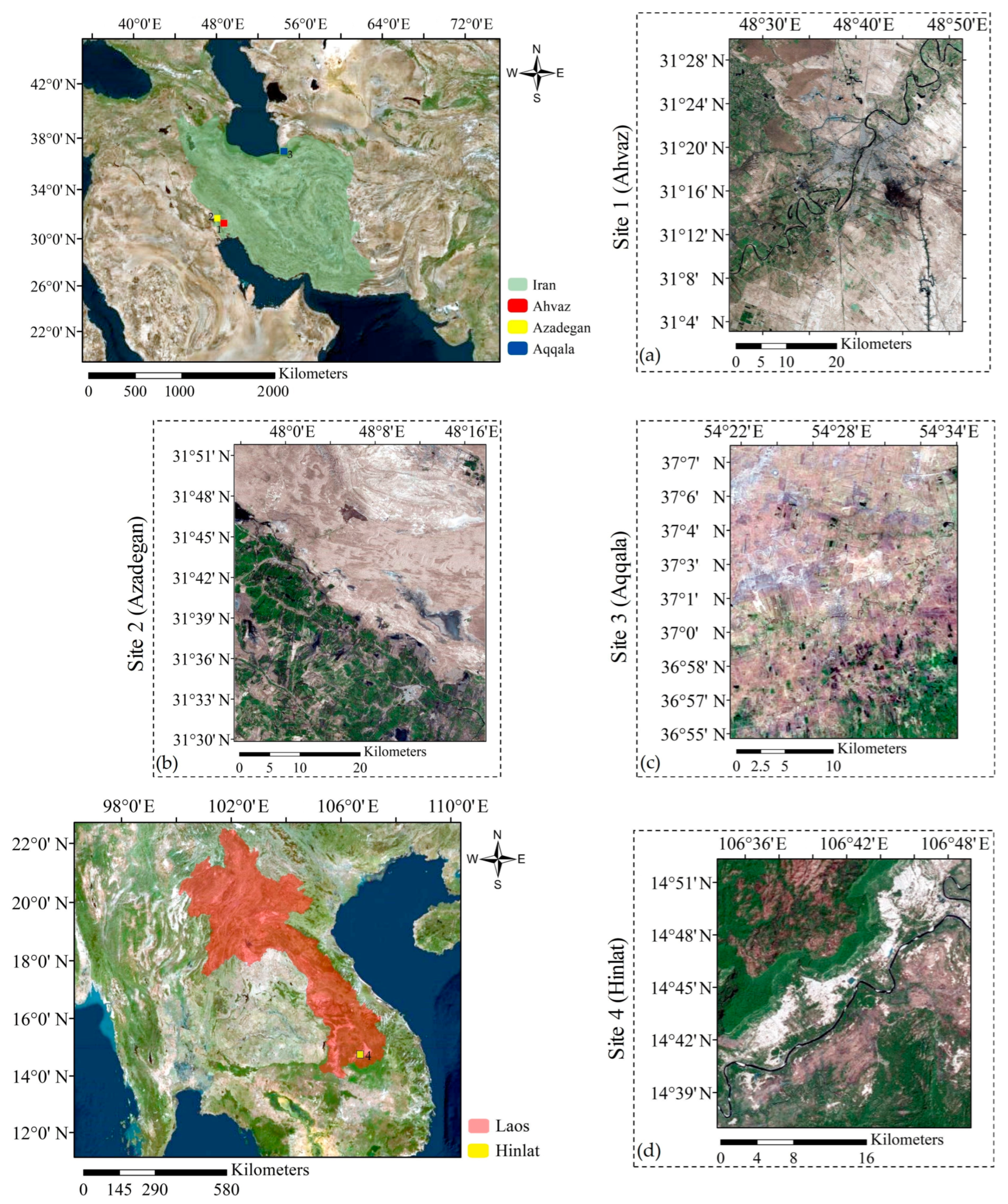
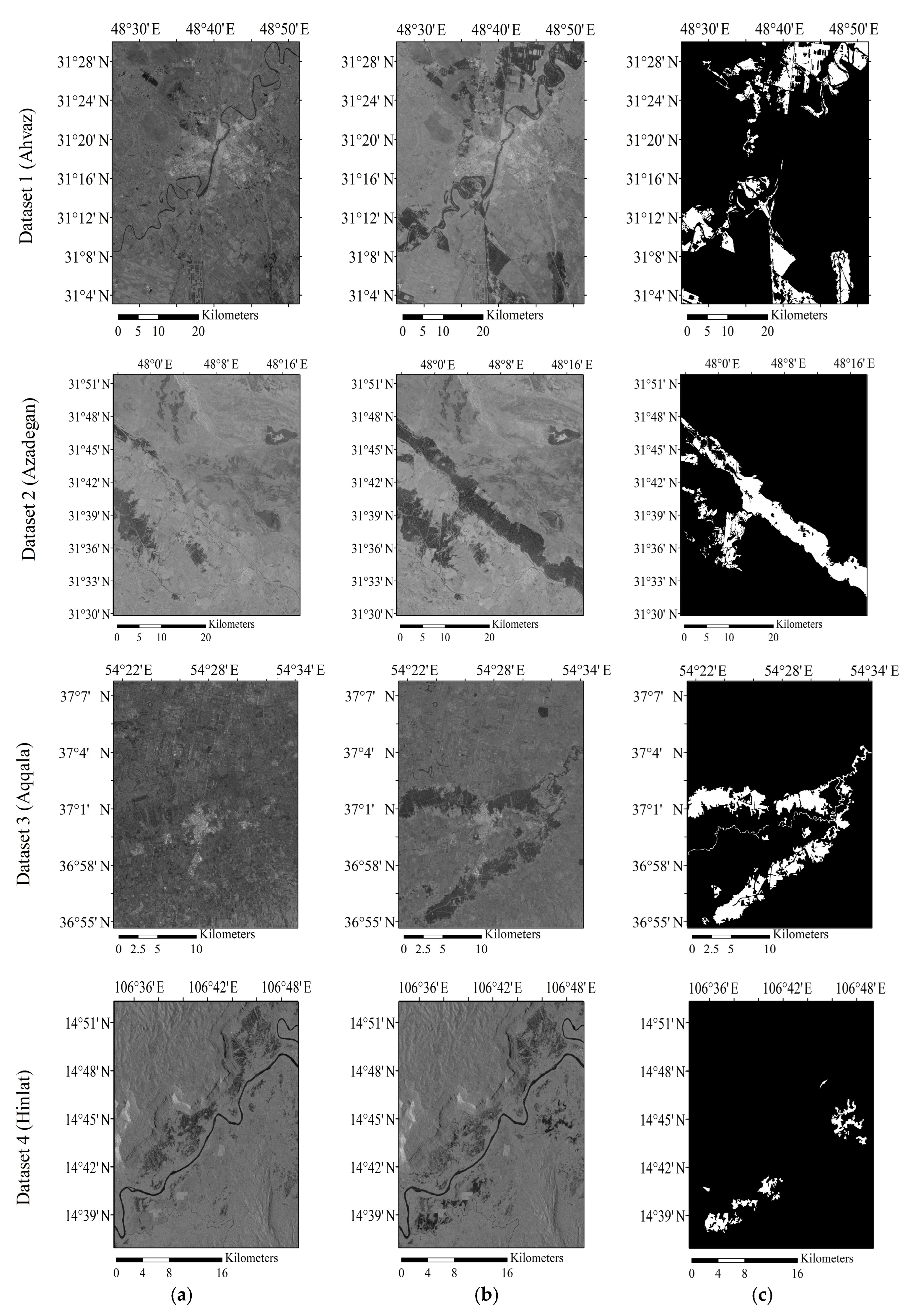
2.2. Study Areas and Datasets

The study areas in this work comprise Ahvaz, Dasht-e Azadegan (Azadegan), and Aqqala in Iran (Figure 2a), as well as the Hinlat area in Laos (Figure 2b). The Karun River, flowing through Khuzestan province in Iran, flooded on 29 March 2019, after a heavy rainfall, which caused significant damage in Ahvaz and Azadegan. These two sites cover approximately 1794.940 and 1311.638 (km2) of land, respectively, with average elevations of 15.98 (m) and 29.637 (m) above sea level. On 19 March 2019, the Aqqala site in Iran’s Golestan province was affected by a severe flood due to continuous heavy rainfall that lasted for several days. The site occupies approximately 431.280 (km2) of land and also has an average land elevation of −12.503 (m), i.e., 12.503 (m) below sea level.
In Laos, the Xe-Namnoy dam in the Champasak Province collapsed, and a huge volume of water flowed along the Vang Nagao River, resulting in a devastating flood in the Hinlat site. The Hinlat site is located on the south side of the dam and the river, covering approximately 801.383 (km2) with an average land elevation of 334.751 (m).
Importantly, these study areas vary in geographical region, land cover, surface roughness, spatial coverage, area of flooded region, and topography conditions, allowing for the assessment of the generalizability and flexibility of the proposed flood mapping approach.
In this study, the dataset for each site includes pre- and co-flood SAR Sentinel-1 (S1) data, pre-flood S2 image, Slope, and ground truth data. To gather the pre- and co-flood S1 data for detecting floodwaters, level-1 interferometric wide swath (IW) ground range detected (GRD) data with a spatial resolution of 10 (m) were obtained from the Google Earth Engine (GEE) platform (“COPERNICUS/S1_GRD”). The VV polarization of S1 data was selected here since it offers a more reasonable and accurate representation of the flooded area [58,59,60]. S1 data on GEE has also already been preprocessed by the Sentinel-1 toolbox that carries out (1) orbital error correction, (2) GRD border noise removal, (3) thermal noise removal, (4) radiometric calibration, and (5) orthorectification. In SAR data, speckle noise is an inherent issue caused by the destructive and constructive interference of the individual reflectors in each ground resolution cell. This noise appears with a “salt and pepper” pattern, decreasing the quality and interpretability of the image. To diminish the adverse impact of the speckle noise, the refined Lee filter, to preserve image details [61], was used in the Sentinel Application Platform (SNAP v.9.0). SNAP is an open-source toolbox developed by the European Space Agency (ESA) for processing Sentinel-1 data. To remove pixels in areas where flooding is topographically improbable, the slope data were obtained from the Shuttle Radar Topography Mission (SRTM) version 3 “USGS/SRTMGL1_003” offered by NASA JPL on GEE.
Furthermore, the present study exploited Sentinel-2 (S2) Level-2A orthorectified surface reflectance data, available as (“COPERNICUS/S2_SR_HARMONIZED”) on GEE, to produce and download the NDWI data for masking permanent waters from the flood extent map. S2 data, offering a wide swath width of 290 km, has 13 spectral bands with high spatial resolutions varying from 10 to 60 m. The acquisition time of the pre-flood S2 data used for generating the NDWI image was chosen close to the flooding date, implying the water level of permanent waters was beneath the alert level. Additionally, this temporal consideration enables precisely removing permanent waterbodies, ensuring a satisfactory distinction between permanent waters and floodwaters.
As the last item in each dataset, a reference flood extent map (ground truth data) was generated manually through meticulous visual inspections between the pre- and co-flood S1 images to validate flood extent maps based on the quantitative evaluation metrics. Table 1 and Figure 3 present further information on the datasets used in this research.

2.3. Performance Evaluation Metrics

To quantitatively appraise the performance of the comparative unsupervised change detection methods, four numeric criteria, including recall ( M r ), precision ( M p ), F-score ( F s ), and intersection over union ( I o U ) were used in this study. M r and M p are individual assessment metrics measuring how effective an algorithm is in classifying flood and non-flood pixels, respectively. The F s metric, however, is a combined metric calculated based on the former metrics, revealing the trade-off (balance) between M r and M p [62]. Additionally, I o U measures the overlapping area between the flood map and the ground truth data. These quantitative metrics are calculated as follows [63,64]:
M r = T P T P + F N
M p = T P T P + F P
F s = 2 × M r × M p M r + M p
I o U = T P T P + F N + F P
where T P , F P , T N , and F N represent the numbers of true positives, false positives, true negatives, and false negatives in the confusion matrix attained by comparing the flood extent map to the ground truth data according to Table 2.

3. Results

3.1. Parameter Setting

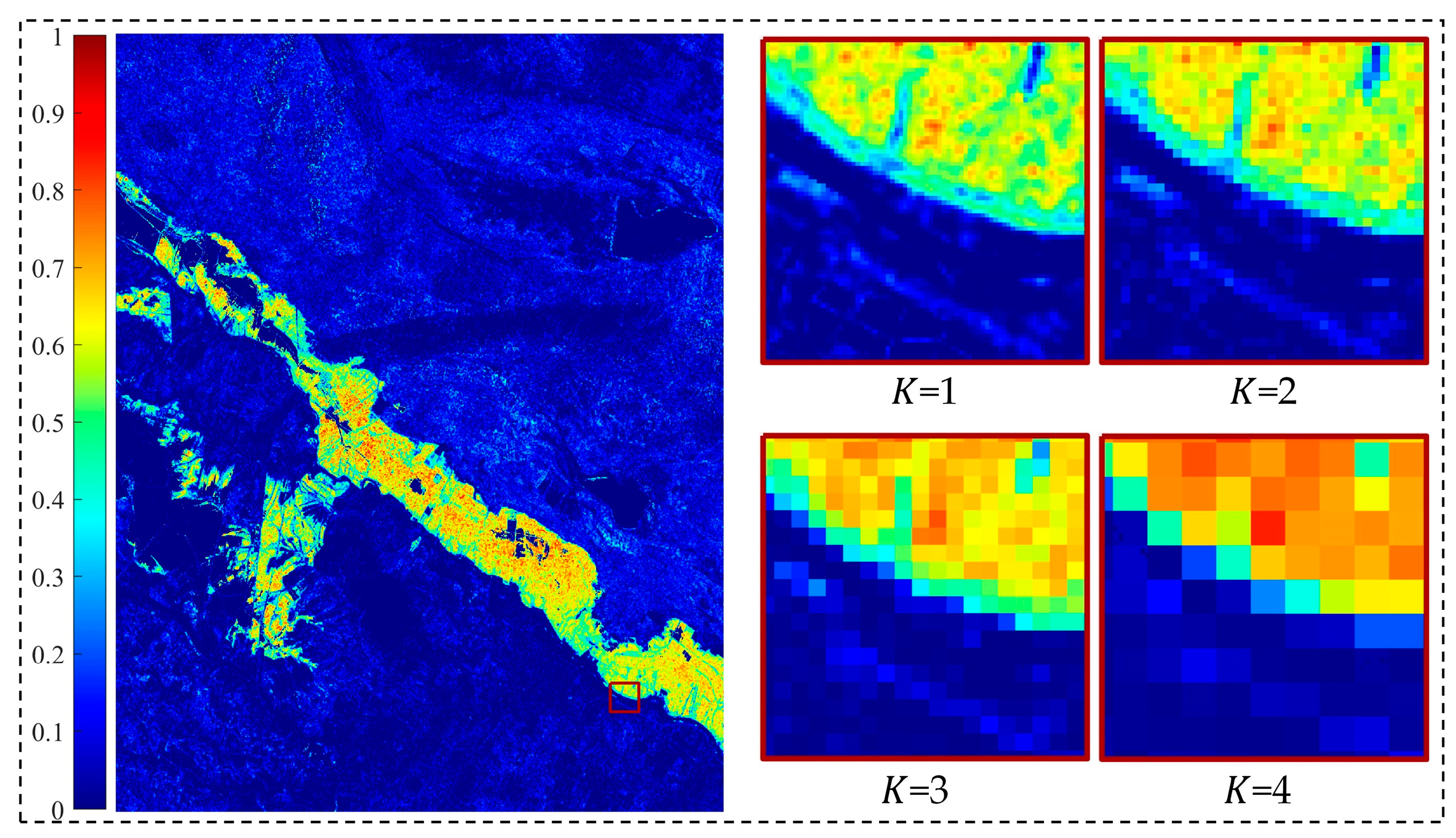
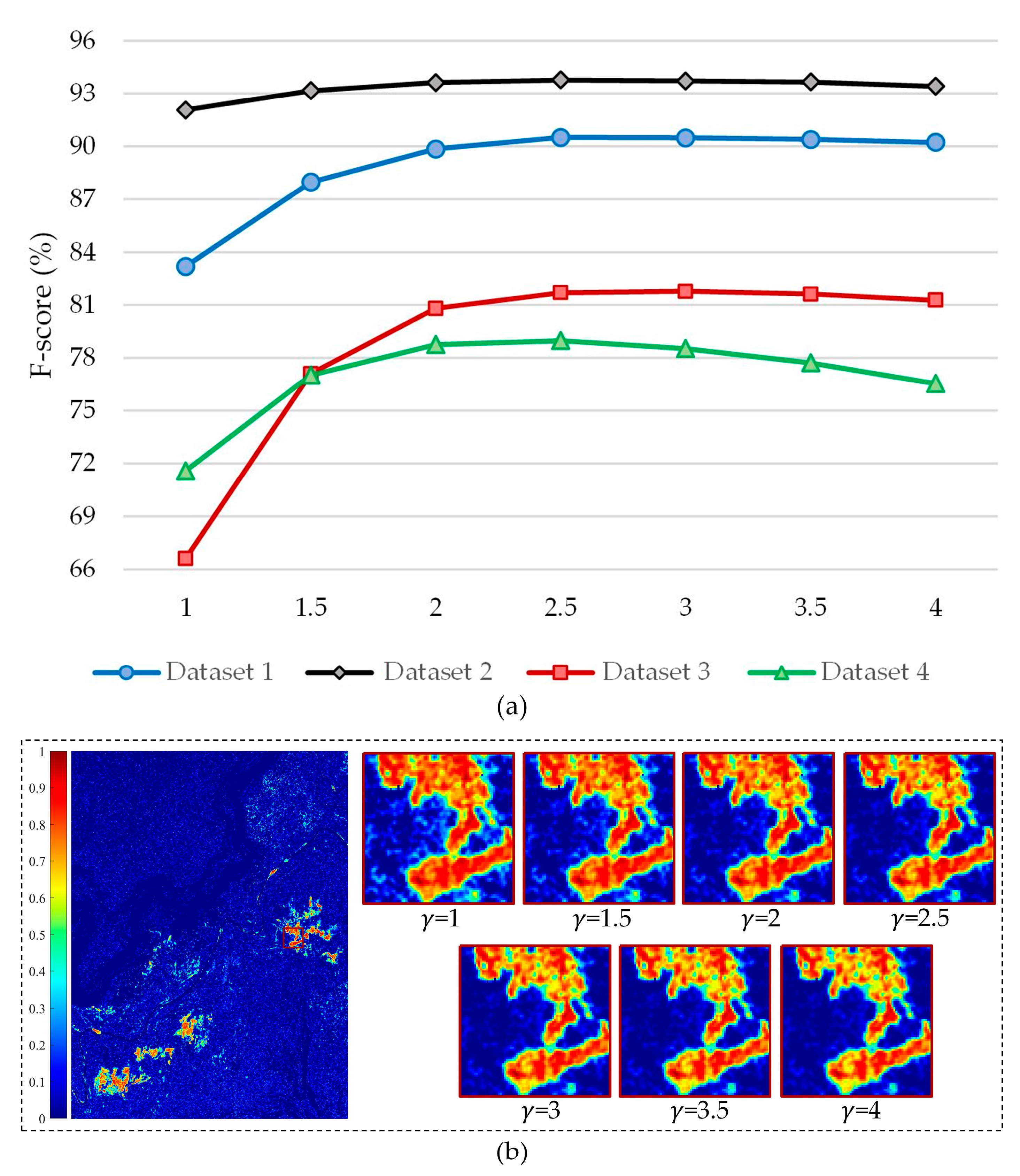
3.1.1. Level of Decomposition (K) and Intensity Transform ( γ ) Parameters in IWFCI

The decomposition level parameter (K) in the DWT fusion technique specifies how many times change indices are successively divided into lower-resolution sub-bands. Figure 4 illustrates how this parameter influences the flood change information in the proposed IWFCI for the red close-up on the CI of dataset 2.
Furthermore, the intensity transform parameter ( γ ) in the proposed fused CI is a paramount parameter regulating background noise suppression in the fusion process. A small value of the parameter diminishes the artifacts and spurious flood changes to a slight degree, while a high one may weaken the real flood changes. Here, to investigate the sensitivity of the IWFCI to the γ parameter, the quantitative and qualitative results of the proposed CI were obtained for the γ values ranging from 1 to 4 and (Figure 5). Figure 5b illustrates the impact of the parameter on flood change information over a crop of dataset 4.

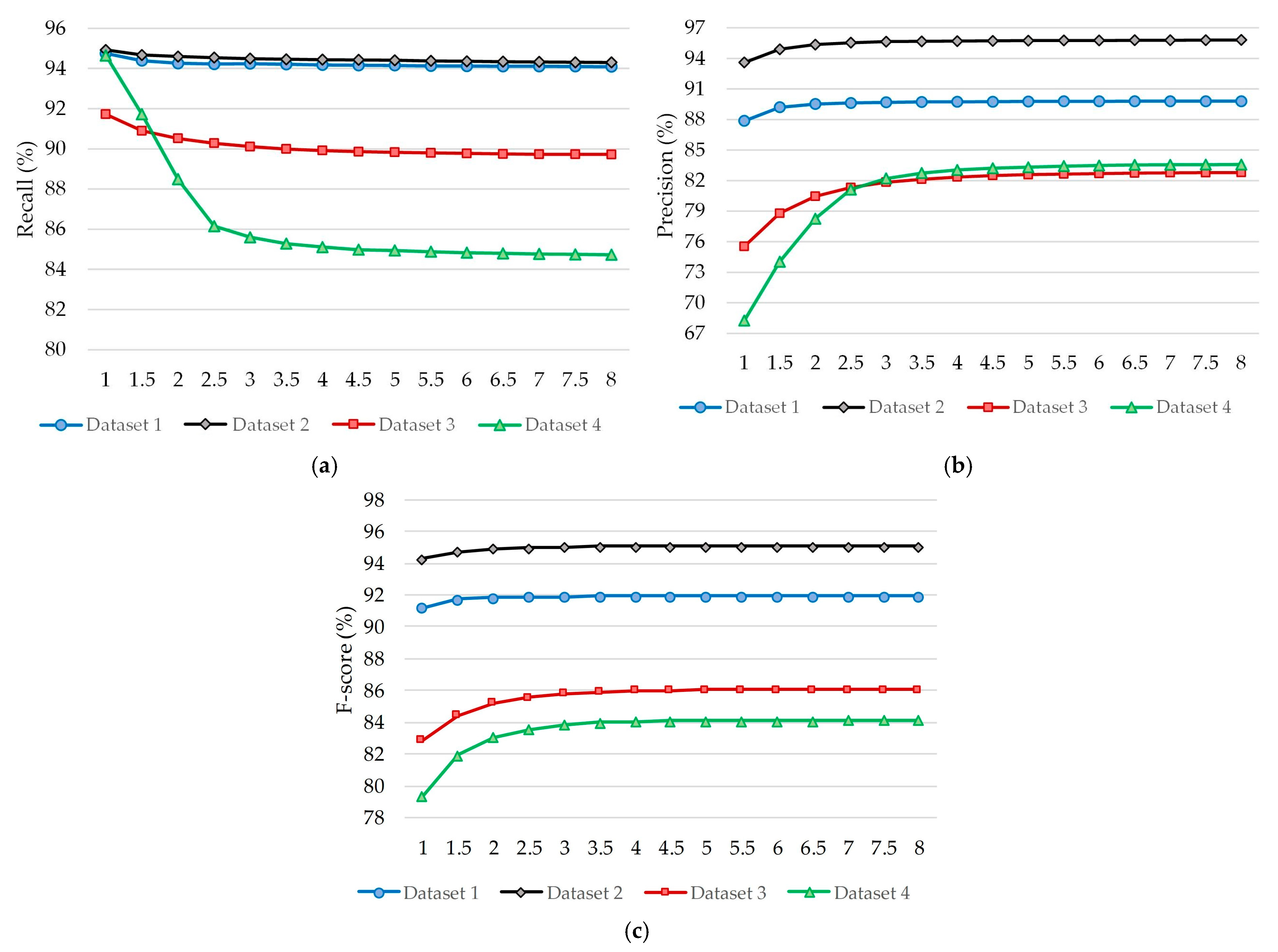
3.1.2. β Parameter in the USMRF Model

The spatial weight ( β ) in MRF-based models tunes the contribution of spatial context (smoothness) to generating the flood extent map. In detail, as the spatial weight parameter takes large values, the inherent smoothness of the proposed USMRF decreases, which, therefore, reduces the over-predictions in labeling flood information. In contrast, a small value of β causes a high smoothness and makes the flooded area over-smoothed, removing change details in the flood extent map. In this work, to evaluate the impact of β and how stable USMRF remains against different values of that, the Fs, recall, and precision values of the model were attained for β values varying from 1 to 8 (Figure 6).

3.2. Evaluating the Proposed Flood Change Index

In this study, to investigate the efficiency of the proposed IWFCI in representing flooded areas, it was compared quantitatively and visually with a number of conventional change indices, including log-ratio (LR), mean-ratio (MR), normalized difference flood index (NDFI) [30], and wavelet-fusion change index (WFCI) [37]. Figure 7 demonstrates the quantitative results attained by the Otsu thresholding-based segmentation of the compared CIs, and flood CIs are visually depicted in Figure 8.

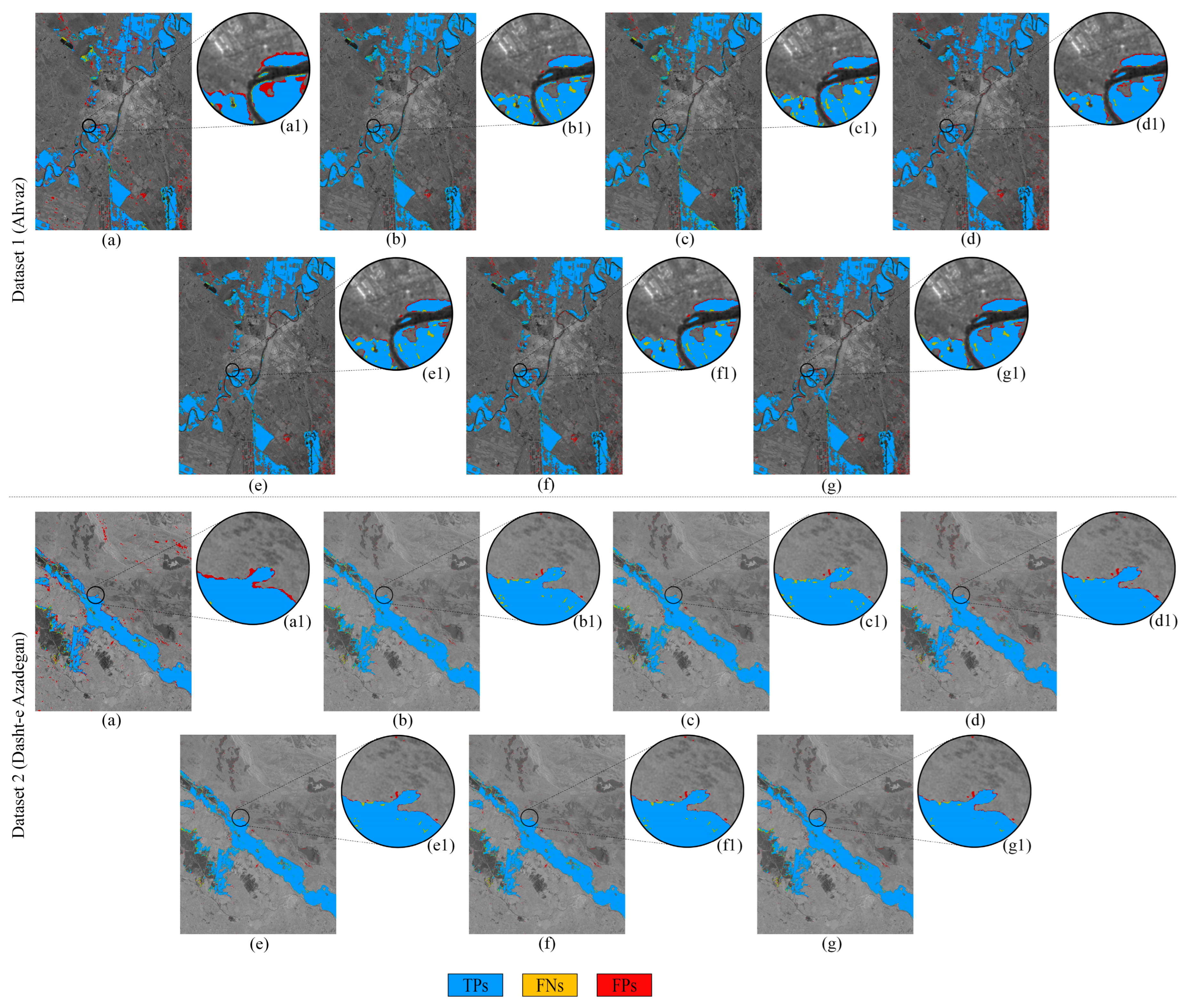
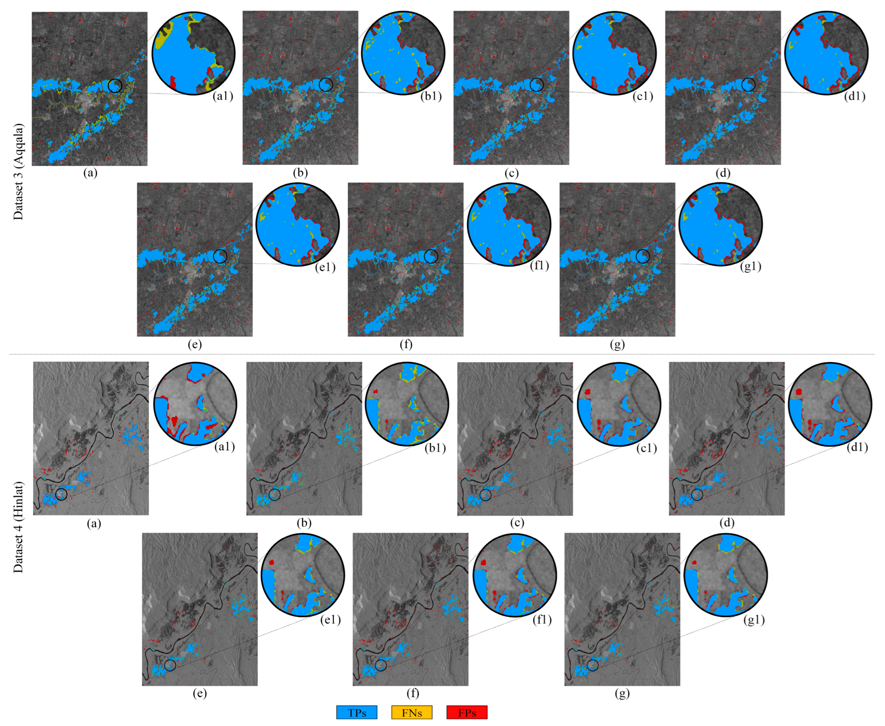
3.3. Assessment of the Proposed USMRF Model

In this work, the proposed USMRF model was compared in quantitative and qualitative results to a supervised approach and five conventional UCD algorithms, including PCAkmeans [65], distribution-based thresholding (DBT) [30], MRF, local uncertainty MRF (LUMRF) [52], and iterative feedback-based thresholding (IFBT) [16]. In PCAkmeans, the parameter h was set to 3. For the DBT approach, the value of k was considered 1.5 based on trial and error. In addition, the kernel sizes for the dilation and closing processes were 3 × 3. Spurious flood clusters smaller than 10 pixels were removed as well. In MRF and LUMRF, β was taken as 5 and 2.5, respectively. The parameters used in IFBT were also chosen as V = 1.1 , Z = 1.1 , and = 3 . All the UCD methods were applied to the same change index proposed in this study for impartial comparison. Additionally, the performance of the proposed approach was compared to the three-dimensional convolutional neural network (3D-CNN) as a supervised deep learning (DL) model [66]. The 3D-CNN model captures multi-temporal SAR images to identify flooded areas based on two convolutional layers. In 3D-CNN, the learning rate and number of epochs were set to 0.001 and 100, respectively, and the adaptive moment estimation (ADAM) was also used as the optimizer in the training phase. The quantitative and qualitative results obtained from the comparative methods are reported in Table 3 and Figure 9 and Figure 10.

4. Discussion

4.1. Performance of the Proposed IWFCI in Reflecting Flood Changes

The level of decomposition and the intensity transform ( γ ) are the two parameters used in the proposed fused CI. As evident from Figure 4, the higher the level of decomposition, the more the spatial resolution decreases, causing adverse blocky artifacts and removing the details of the flood change information in the fused CI. Accordingly, to best preserve the spatial resolution and the details of flood change information, the K value was set to 1 in this study.
According to Figure 5a, the trend of F-score change in all cases was almost the same, where the F-score values initially increased and then decreased after a particular value. In more detail, on datasets 1 and 3, the proposed IWFCI performed best when the γ value was set to 3, whereas the highest F-score values on datasets 2 and 4 were achieved for γ = 2.5. This is probably because the background of the proposed fused CI on datasets 1 and 3 contained a higher number of artifacts and accordingly required further enhancement than datasets 2 and 4. Nevertheless, the IWFCI demonstrated a satisfactory, reliable performance in all cases for γ = 2, 2.5, and 3 with slight variations. In addition, the maximum and minimum noise were observed for γ = 1 and γ = 4, respectively (Figure 5b). The change intensities related to real flood information also diminished as the γ values increased, which reveals why the performance of IWFCI degraded for the high values of γ in Figure 5a. Indeed, high values of the parameter can cause harm to the main change intensities, which leads the fused CI to lose some real flood information. Indeed, a suitable value for γ is the one that enables the IWFCI to achieve high accuracy by balancing noise suppression and reflecting real changes. This was observed across multiple datasets, which varied in different aspects, when γ was set to 2.5 (Figure 5), implying the flexibility of the proposed CI in diverse scenarios. Therefore, the γ parameter in the proposed IWFCI is recommended to be set to 2.5.
As observed in Figure 7, the proposed IWFCI showed the highest efficacy in generating flood extent maps on all datasets, confirming its superiority over the other CIs. For instance, for dataset 1, IWFCI with an IoU of 82.56% improved LR, MR, ND, and WFCI by 5.82%, 50.69%, 29.89%, and 31.14%, respectively. In addition, for dataset 4, IWFCI led to an Fs value of 78.98%, raising those of LR, MR, ND, and WFCI by 3.27%, 57.15%, 25.15%, and 20.40%, respectively. Compared to the traditional WFCI, which performed better than MR and ND only on datasets 2 and 4, IWFCI revealed the most stable performance in identifying flood pixels across all datasets. Accordingly, the proposed IWFCI, as the most stable and accurate tool, could be used to recognize floodwaters from SAR images in flood mapping applications. The superiority of the proposed flood CI over the other CIs is, firstly, because IWFCI suppresses the background artifacts in MR and only takes its high-magnitude flood changes for the fusion process, making the fused CI less affected by the artifacts. Secondly, the co-flood image, where inundated areas appear as dark pixels, refines the fusion coefficients, enhancing the contrast between the flood and non-flood areas. On the other hand, despite best highlighting severe flood changes, the MR with Fs values of 48.33%, 33.58%, 45.66%, and 21.83% led to the worst quantitative results among the CIs due to many artifacts in its background (non-flood) area.
From the change intensity images represented in Figure 8, in spite of strongly highlighting the flooded area, MR, ND, and WFCI had many artifacts in their background (non-flood) area, which potentially results in over-predictions in flood maps. In contrast, in the log-ratio operator, a minimum number of artifacts were observed, yet change intensities were low due to the logarithmic compression, leading to flood extent maps either missing or over-predicting flood pixels. Among the compared CIs, the proposed IWFCI best decreased the noise and artifacts while amplifying the changed (flooded) areas compared to LR. Accordingly, the proposed IWFCI establishes the highest distinction between flood and non-flood classes, which can consequently produce more accurate flood maps.

4.2. Performance of the Proposed USMRF Model in Generating Flood Maps

As mentioned previously, the spatial weight ( β ) parameter influences the performance of the proposed approach in detecting flooded areas. As depicted in Figure 6, USMRF demonstrated a similar precision/Fs trend across all datasets with raising β , where the precision/Fs values were low in the beginning, implying the model overly caused smoothness (i.e., many FPs) to the flood objects for small β values. In contrast, high recall values were obtained when β was set to low values (Figure 6a), revealing that the model produced more homogenous flood objects with fewer FNs. However, the higher the spatial weight value ( β ), the less smoothness the model introduces to the flood objects, resulting in more FNs and lower recall values. On the other hand, as the values of spatial weight increased, the number of FPs decreased, leading the precision/Fs values to improve and achieve stability once β reached 5, where the model balanced the integration of change intensities and spatial context information. The β value of 5, for which the model reached stability in all cases, is recommended for use in the proposed USMRF model. Importantly, despite the diversity of the multiple datasets in the form of land cover, topography, spatial coverage, and the area of flood class, the proposed model exhibited high accuracy and stable performance in various cases. This indicates the generalizability of the proposed approach in detecting floodwaters over different geographical regions.
As for the quantitative comparison made among the different methods, according to Table 3, the proposed USMRF model exhibited the best performance in Fs and IoU criteria across all datasets compared to the other methods. For example, USMRF with an Fs of 84.1% on dataset 4 improved 3D-CNN, PCAkmeans, DBT, MRF, LUMRF, and IFBT by 1.09%, 3.93%, 6.36%, 4.65%, 1.88%, and 4.17%, respectively. Similarly, the IoU values of 3D-CNN, PCAkmeans, DBT, MRF, LUMRF, and IFBT on dataset 2 were enhanced by 11.65%, 1.28%, 1.73%, 1.58%, 0.59%, and 0.68% when using the USMRF model for segmenting the IWFCI. Regarding the performance of models in classifying either of flooded and non-flooded areas separately, PCAkmeans with maximum/minimum values of TNs/FPs on datasets 2 and 4 performed better than the other algorithms, yielding the highest precision values of 96.78% and 85.2%, respectively. Furthermore, on datasets 1 and 3, the best precision values of 93.62% and 88.81% were attained by the DBT and 3D-CNN approaches, respectively. Nevertheless, 3D-CNN showed an underperformance in detecting the non-flood class with the least TNs of 15,079,349 and 11,417,982 and maximum FPs of 529,877 and 285,073 on datasets 1 and 2, respectively, reaching low precision values of 80.74% and 82.47%. On the other hand, in terms of extracting the flooded areas, best performance on datasets 1–4 corresponds to MRF with TPs/recall of 2,232,011/95.38%, 1,345,528/95.2%, 397,815/91.39%, and 132,797/94.65%, respectively, which is a result of the over-smoothness producing homogenous flood objects. However, in identifying the non-flood class, the over-smoothness in MRF caused low precision values. In contrast to MRF, the LUMRF, IFBT, and USMRF models reduced the FPs, resulting in higher precision values. Additionally, of these three methods, the proposed USMRF separated the flood and non-flood classes more accurately besides balancing the recall and precision values. Specifically, on dataset 1, USMRF yielded TPs/recall of 2,203,538/94.16% with improvements of 15,936/0.68% and 23,366/1.00% compared to LUMRF and IFBT, respectively. Analogously, the FNs of IFBT and LUMRF on dataset 3 decreased by 6,063 and 2,927 pixels, respectively, when employing USMRF for mapping floodwaters. This is because the model tunes the smoothness in diverse areas based on small penalty coefficients (high smoothness) in certain areas and large coefficients (low smoothness) in uncertain regions.
Moreover, investigating the accuracy values of the proposed approach, the method showed variations across different datasets, which could be due to their differences in (1) regional characteristics, (2) SAR backscatter, and (3) image size (i.e., spatial coverage) and the area of flood class. Datasets used in the present work include different geographical regions varying in land cover, surface roughness, and topography, which can impact flood changes and lead to varying accuracies in detecting floodwaters accordingly. Furthermore, SAR backscatter differences between the pre-flood and co-flood images vary across different datasets, possibly leading to discrepancies in their accuracy. The image size and the area of flood class are also thought to contribute to accuracy variation. The combined quantitative metrics, such as Fs and IoU, are calculated based on TPs, FNs, and FPs and are directly related to TPs. These criteria, especially TPs, depend highly on the image size and the area of flood class. Indeed, the larger the flooded area in a dataset, the higher the TPs in the quantitative assessment. In further detail, from Table 3, the lowest accuracies were obtained on datasets 3 and 4 due to their low TPs, whereas the highest values correspond to datasets 1 and 2, indicating that the difference in the image size and area of flood class can cause discrepancies in the accuracy across different datasets.
Based on the qualitative results shown in Figure 9 and Figure 10, the DL-based 3D-CNN model, despite yielding homogeneous flood objects, tended to either underestimate or overestimate the flood extent. This could be due to the few convolutional layers in 3D-CNN, preventing the model from learning more complicated and detailed flood features. In contrast, PCAkmeans resulted in the flood maps containing few over-predictions but missed many flood pixels inside the flood objects. Compared to PCAkmeans, the number of under-predictions in DBT flood maps decreased slightly; however, this method either failed to extract some flood pixels or led to many over-predictions despite employing the morphological procedures. The reason is that both approaches do not integrate change intensity with spatial context, although they consider the neighboring intensity information. Conversely, MRF delineated more homogeneous pixels by integrating the change intensity with spatial context but resulted in many FPs as over-predictions due to the over-smoothness issue. In contrast, the flood maps obtained from the IFBT method contained fewer FPs but could not recognize some of the flood pixels inside the flooded area. Compared to MRF, the contribution of spatial context to the segmentation of change index in LUMRF varies in the local uncertain areas, leading to fewer FPs in identifying flooded areas. Nevertheless, similar to the IFBT approach, the model missed some flood pixels as the performance of LUMRF is highly restricted to the membership degrees of the fuzzy c-means algorithm. In contrast to LUMRF and IFBT, the proposed USMRF algorithm resulted in the change maps extracting more flood pixels in most parts of the flooded area while reducing FPs compared to MRF. Indeed, the flood maps attained by USMRF balanced the number of FNs and FPs better than the other flood mapping methods, further confirming the superiority of the proposed approach in detecting flooded areas based on SAR Sentinel-1 data.
Despite the advantages of SAR Sentinel-1 data in flood mapping, some uncertainties may lead to underestimating the floodwaters in dense vegetation or overestimating the flood pixels in areas affected by radar shadowing, a common topography-related issue in SAR data.
On the one hand, in densely vegetated areas, Sentinel-1 data have a limited penetration due to operating at short C-band frequency, causing some uncertainties that may result in underestimating flooded areas. First, SAR signals may be scattered before reaching the floodwater, providing no information about whether the area beneath the vegetation is inundated. Second, regarding the shallow floodwaters in dense vegetation such as agricultural areas, the backscatter intensity slightly changes, which cannot be recognized properly and may also be confused with the backscatter change related to soil moisture increase, especially in rainfall-related flooding. Hence, the proposed flood detection method cannot detect the floodwater beneath the dense vegetation. However, according to Figure 11, the approach can detect floodwaters submerging the short dense vegetation as illustrated in the close-up depiction on dataset 3 (Aqqala site). The close-up area with a mean normalized difference vegetation index (NDVI) of 0.79, estimated from the pre-flood Sentinel-2 data, corresponds to the dense vegetation of agricultural type in Aqqala where farmlands dominate the region.
On the other hand, owing to the side-looking imaging geometry, the SAR antenna receives no signal from the terrains with steep slopes obscured from the view of the sensor. As a result, radar shadowing error occurs over these areas, appearing in a dark tone similar to floodwaters, which can overestimate flood pixels. To examine how the proposed method deals with this challenge, a close-up on dataset 4 was illustrated in Figure 12, where dark areas show shadows and smooth surfaces. Dataset 4, i.e., the Hinlat area, is characterized by a diverse topography, including flat plains, smooth areas, and elevated regions. According to Figure 12, the proposed approach minimizes the number of errors (FPs) over radar shadows and smooth surfaces. This confirms that the proposed flood CI can satisfactorily distinguish the floodwaters from water-like surfaces.

5. Conclusions

In the present study, a novel unsupervised floodwater mapping approach, consisting of an improved wavelet-fusion flood-change index (IWFCI) and an uncertainty-sensitive MRF (USMRF) model, was proposed to identify floods in rural areas. To construct the IWFCI, a discriminant flood feature was generated from the flood image to enhance the separability between the non-flood and flood classes in the fusion process. Thereafter, the mean-ratio change index (CI) was modified using the Gamma intensity transform to weaken its noisy changes and their adverse impact on the fusion result. The discrete wavelet transform (DWT) algorithm was finally employed to integrate the modified mean-ratio change index, log-ratio change index, and the flood feature. To devise the USMRF model for classifying the IWFCI into non-flood and flood classes, a Gaussian uncertainty penalty term was proposed and incorporated into the model to mitigate the over-smoothness issue around the separation point of the two classes, regarded as the uncertainty area.
In the present study, three sites in Iran and one site in Laos were considered to investigate the efficiency of the proposed floodwater recognition method. In order to conduct the experiments in two evaluation stages, the dataset corresponding to each study area comprised pre-flood and co-flood Sentinel-1 images, slope data calculated from the digital elevation model, and the normalized difference water index (NDWI) derived from the Sentinel-2 data acquired before the flooding. In the first stage, the proposed IWFCI was compared to the state-of-the-art (SOTA) individual and fused CIs, and the second stage intended to compare the proposed USMRF model with the SOTA change detection and flood mapping methods. According to the results obtained in the first stage, the proposed IWFCI with an average F-score of 86.20% performed best in quantitative results compared to the SOTA CIs. From qualitative results, IWFCI had a background with minimum noise and artifacts due to suppressing the noise in the background of the mean-ratio CI using the Gamma intensity transform. Moreover, incorporating the flood image-derived feature into the fusion process enhanced the contrast between the non-flooded and flooded areas. As for the results in the second stage, in the flood extent maps attained by USMRF, the number of false positives (over-predictions) decreased compared to the typical MRF in the uncertain inter-class areas. Also, USMRF, due to better balancing the recall and precision metrics, yielded an average F-score of 89.27%, outperforming the SOTA methods in distinguishing flood pixels from non-flood pixels. Further evaluations in densely vegetated areas showed the approach can identify floodwaters submerging the dense vegetation but cannot recognize shallow floods beneath dense vegetation. As for the water-like surfaces, visual analyses on a complex topography revealed that the proposed method led to a minimum number of FPs (over-predictions) in both smooth areas and topography-induced shadows. In general, it can be deduced that the proposed SAR CD-based approach, combining the IWFCI and USMRF, is a reliable, accurate method to identify rural floodwaters in all-time, all-weather conditions. The proposed method can also be generalized to other flood events due to its stable, superior performance under various geographical, topographical, and hydrological conditions.
As a beneficial SAR data-based feature, the IWFCI could also be used in forthcoming multi-source (SAR-optical fusion-based) floodwater detection studies. The intensity transform parameter ( γ ) in the proposed fused flood CI (i.e., IWFCI) and the spatial weight parameter ( β ) in the USMRF model, which were empirically determined in this study, seem to work for other rural flood events as well. However, further appraisal of their stability and automatic determination could be carried out in future efforts in the field of rural flood detection.

Author Contributions

Conceptualization, A.M. (Amin Mohsenifar), A.M. (Ali Mohammadzadeh) and S.J.; methodology, A.M. (Amin Mohsenifar) and A.M. (Ali Mohammadzadeh); investigation, all authors; writing—original draft preparation, A.M. (Amin Mohsenifar); writing—review and editing, all authors; visualization, A.M. (Amin Mohsenifar); supervision, A.M. (Ali Mohammadzadeh) and S.J.; Funding acquisition, S.J. All authors have read and agreed to the published version of the manuscript.

Funding

This research received no external funding.

Data Availability Statement

The datasets used in this article are unavailable since the data are part of an ongoing study.

Acknowledgments

The authors would like to appreciate LiDAR research laboratory of K. N. Toosi University of Technology, Tehran, Iran. They would also like to express their sincere gratitude to Sahand Tahermanesh and Armin Moghimi for their guidance. Amin Mohsenifar was also supported by the Erasmus+ ICM Student Mobility Programme for six months at Lund University, Sweden. Sadegh Jamali was partly supported by the Development Research Grant 2024–2025 from the Faculty of Engineering (LTH) at Lund University.

Conflicts of Interest

The authors declare no conflicts of interest.

References

  1. Addabbo, A.D.; Refice, A.; Pasquariello, G.; Lovergine, F.P.; Capolongo, D.; Manfreda, S. A Bayesian Network for Flood Detection Combining SAR Imagery and Ancillary Data. IEEE Trans. Geosci. Remote Sens. 2016, 54, 3612–3625. [Google Scholar] [CrossRef]
  2. Rosser, J.F.; Leibovici, D.G.; Jackson, M.J. Rapid flood inundation mapping using social media, remote sensing and topographic data. Nat. Hazards 2017, 87, 103–120. [Google Scholar] [CrossRef]
  3. Li, Y.; Martinis, S.; Wieland, M.; Schlaffer, S.; Natsuaki, R. Urban flood mapping using SAR intensity and interferometric coherence via Bayesian network fusion. Remote Sens. 2019, 11, 2231. [Google Scholar] [CrossRef]
  4. Ulloa, N.I.; Yun, S.-H.; Chiang, S.-H.; Furuta, R. Sentinel-1 Spatiotemporal Simulation Using Convolutional LSTM for Flood Mapping. Remote Sens. 2022, 14, 246. [Google Scholar] [CrossRef]
  5. Farhadi, H.; Ebadi, H.; Kiani, A.; Asgary, A. Introducing a new index for flood mapping using Sentinel-2 imagery (SFMI). Comput. Geosci. 2024, 194, 105742. [Google Scholar] [CrossRef]
  6. Li, Y.; Martinis, S.; Plank, S.; Ludwig, R. An automatic change detection approach for rapid flood mapping in Sentinel-1 SAR data. Int. J. Appl. Earth Obs. Geoinf. 2018, 73, 123–135. [Google Scholar] [CrossRef]
  7. Feng, Q.; Gong, J.; Liu, J.; Li, Y. Flood Mapping Based on Multiple Endmember Spectral Mixture Analysis and Random Forest Classifier-The Case of Yuyao, China. Remote Sens. 2015, 7, 12539–12562. [Google Scholar] [CrossRef]
  8. DeVries, B.; Huang, C.; Armston, J.; Huang, W.; Jones, J.W.; Lang, M.W. Rapid and robust monitoring of flood events using Sentinel-1 and Landsat data on the Google Earth Engine. Remote Sens. Environ. 2020, 240, 111664. [Google Scholar] [CrossRef]
  9. Farhadi, H.; Esmaeily, A.; Najafzadeh, M. Flood monitoring by integration of Remote Sensing technique and Multi-Criteria Decision Making method. Comput. Geosci. 2022, 160, 105045. [Google Scholar] [CrossRef]
  10. Khankeshizadeh, E.; Tahermanesh, S.; Mohsenifar, A.; Moghimi, A.; Mohammadzadeh, A. FBA-DPAttResU-Net: Forest burned area detection using a novel end-to-end dual-path attention residual-based U-Net from post-fire Sentinel-1 and Sentinel-2 images. Ecol. Indic. 2024, 167, 112589. [Google Scholar] [CrossRef]
  11. Shastry, A.; Carter, E.; Coltin, B.; Sleeter, R.; McMichael, S.; Eggleston, J. Mapping floods from remote sensing data and quantifying the effects of surface obstruction by clouds and vegetation. Remote Sens. Environ. 2023, 291, 113556. [Google Scholar] [CrossRef]
  12. Lang, F.; Zhu, Y.; Zhao, J.; Hu, X.; Shi, H.; Zheng, N.; Zha, J. Flood Mapping of Synthetic Aperture Radar (SAR) Imagery Based on Semi-Automatic Thresholding and Change Detection. Remote Sens. 2024, 16, 2763. [Google Scholar] [CrossRef]
  13. Schlaffer, S.; Chini, M.; Giustarini, L.; Matgen, P. Probabilistic mapping of flood-induced backscatter changes in SAR time series. Int. J. Appl. Earth Obs. Geoinf. 2017, 56, 77–87. [Google Scholar] [CrossRef]
  14. Voormansik, K.; Praks, J.; Antropov, O.; Jagomagi, J.; Zalite, K. Flood mapping with terraSAR-X in forested regions in estonia. IEEE J. Sel. Top. Appl. Earth Obs. Remote Sens. 2014, 7, 562–577. [Google Scholar] [CrossRef]
  15. Chini, M.; Hostache, R.; Giustarini, L.; Matgen, P. A hierarchical split-based approach for parametric thresholding of SAR images: Flood inundation as a test case. IEEE Trans. Geosci. Remote Sens. 2017, 55, 6975–6988. [Google Scholar] [CrossRef]
  16. Zhao, M.; Ling, Q.; Li, F. An Iterative Feedback-Based Change Detection Algorithm for Flood Mapping in SAR Images. IEEE Geosci. Remote Sens. Lett. 2019, 16, 231–235. [Google Scholar] [CrossRef]
  17. Sui, H.; An, K.; Xu, C.; Liu, J.; Feng, W. Flood Detection in PolSAR Images Based on Level Set Method Considering Prior Geoinformation. IEEE Geosci. Remote Sens. Lett. 2018, 15, 699–703. [Google Scholar] [CrossRef]
  18. Jamali, A.; Roy, S.K.; Hashemi Beni, L.; Pradhan, B.; Li, J.; Ghamisi, P. Residual wave vision U-Net for flood mapping using dual polarization Sentinel-1 SAR imagery. Int. J. Appl. Earth Obs. Geoinf. 2023, 127, 103662. [Google Scholar] [CrossRef]
  19. Shen, X.; Wang, D.; Mao, K.; Anagnostou, E.; Hong, Y. Inundation extent mapping by synthetic aperture radar: A review. Remote Sens. 2019, 11, 879. [Google Scholar] [CrossRef]
  20. Celik, T. Multiscale change detection in multitemporal satellite images. IEEE Geosci. Remote Sens. Lett. 2009, 6, 820–824. [Google Scholar] [CrossRef]
  21. Bruzzone, L.; Prieto, D.F. Automatic analysis of the difference image for unsupervised change detection. IEEE Trans. Geosci. Remote Sens. 2000, 38, 1171–1182. [Google Scholar] [CrossRef]
  22. Bazi, Y.; Bruzzone, L.; Melgani, F. An unsupervised approach based on the generalized Gaussian model to automatic change detection in multitemporal SAR images. IEEE Trans. Geosci. Remote Sens. 2005, 43, 874–887. [Google Scholar] [CrossRef]
  23. Martinis, S.; Twele, A.; Voigt, S. Unsupervised extraction of flood-induced backscatter changes in SAR data using markov image modeling on irregular graphs. IEEE Trans. Geosci. Remote Sens. 2011, 49, 251–263. [Google Scholar] [CrossRef]
  24. Giustarini, L.; Hostache, R.; Matgen, P.; Schumann, G.J.P.; Bates, P.D.; Mason, D.C. A change detection approach to flood mapping in Urban areas using TerraSAR-X. IEEE Trans. Geosci. Remote Sens. 2013, 51, 2417–2430. [Google Scholar] [CrossRef]
  25. Moghimi, A.; Mohammadzadeh, A.; Khazai, S. Integrating Thresholding With Level Set Method for Unsupervised Change Detection in Multitemporal SAR Images. Can. J. Remote Sens. 2017, 43, 412–431. [Google Scholar] [CrossRef]
  26. Kim, Y.; Lee, M.-J. Rapid Change Detection of Flood Affected Area after Collapse of the Laos Xe-Pian Xe-Namnoy Dam Using Sentinel-1 GRD Data. Remote Sens. 2020, 12, 1978. [Google Scholar] [CrossRef]
  27. Natsuaki, R.; Nagai, H. Synthetic aperture radar flood detection under multiple modes and multiple orbit conditions: A case study in japan on typhoon hagibis, 2019. Remote Sens. 2020, 12, 903. [Google Scholar] [CrossRef]
  28. Samuele, D.P.; Federica, G.; Filippo, S.; Enrico, B.-M. A simplified method for water depth mapping over crops during flood based on Copernicus and DTM open data. Agric. Water Manag. 2022, 269, 107642. [Google Scholar] [CrossRef]
  29. Amitrano, D.; Di Martino, G.; Iodice, A.; Riccio, D.; Ruello, G. Unsupervised Rapid Flood Mapping Using Sentinel-1 GRD SAR Images. IEEE Trans. Geosci. Remote Sens. 2018, 56, 3290–3299. [Google Scholar] [CrossRef]
  30. Cian, F.; Marconcini, M.; Ceccato, P. Normalized Difference Flood Index for rapid flood mapping: Taking advantage of EO big data. Remote Sens. Environ. 2018, 209, 712–730. [Google Scholar] [CrossRef]
  31. Vanama, V.S.K.; Rao, Y.S.; Bhatt, C.M. Change detection based flood mapping using multi-temporal Earth Observation satellite images: 2018 flood event of Kerala, India. Eur. J. Remote Sens. 2021, 54, 42–58. [Google Scholar] [CrossRef]
  32. Vekaria, D.; Chander, S.; Singh, R.P.; Dixit, S. A change detection approach to flood inundation mapping using multi-temporal Sentinel-1 SAR images, the Brahmaputra River, Assam (India): 2015–2020. J. Earth Syst. Sci. 2023, 132, 3. [Google Scholar] [CrossRef]
  33. Lu, J.; Giustarini, L.; Xiong, B.; Zhao, L.; Jiang, Y.; Kuang, G. Automated flood detection with improved robustness and efficiency using multi-temporal SAR data. Remote Sens. Lett. 2014, 5, 240–248. [Google Scholar] [CrossRef]
  34. Bovolo, F.; Bruzzone, L. A Split-Based Approach to Unsupervised Change Detection in Large-Size Multitemporal Images: Application to Tsunami-Damage Assessment. IEEE Trans. Geosci. Remote Sens. 2007, 45, 1658–1669. [Google Scholar] [CrossRef]
  35. Mehravar, S.; Razavi-termeh, S.V.; Moghimi, A.; Ranjgar, B.; Foroughnia, F.; Amani, M. Flood susceptibility mapping using multi-temporal SAR imagery and novel integration of nature-inspired algorithms into support vector regression. J. Hydrol. 2023, 617, 129100. [Google Scholar] [CrossRef]
  36. Bovolo, F.; Bruzzone, L. A detail-preserving scale-driven approach to change detection in multitemporal SAR images. IEEE Trans. Geosci. Remote Sens. 2005, 43, 2963–2972. [Google Scholar] [CrossRef]
  37. Gong, M.; Zhou, Z.; Ma, J. Change detection in synthetic aperture radar images based on image fusion and fuzzy clustering. IEEE Trans. Image Process. 2012, 21, 2141–2151. [Google Scholar] [CrossRef]
  38. Wang, J.; Yang, X.; Yang, X.; Jia, L.; Fang, S. Unsupervised change detection between SAR images based on hypergraphs. ISPRS J. Photogramm. Remote Sens. 2020, 164, 61–72. [Google Scholar] [CrossRef]
  39. Moghimi, A.; Khazai, S.; Mohammadzadeh, A. An improved fast level set method initialized with a combination of k-means clustering and Otsu thresholding for unsupervised change detection from SAR images. Arab. J. Geosci. 2017, 10, 293. [Google Scholar] [CrossRef]
  40. Hou, B.; Wei, Q.; Zheng, Y.; Wang, S. Unsupervised change detection in SAR image based on Gauss-log ratio image fusion and compressed projection. IEEE J. Sel. Top. Appl. Earth Obs. Remote Sens. 2014, 7, 3297–3317. [Google Scholar] [CrossRef]
  41. Zheng, Y.; Zhang, X.; Hou, B.; Liu, G. Using combined difference image and k-means clustering for SAR image change detection. IEEE Geosci. Remote Sens. Lett. 2013, 11, 691–695. [Google Scholar] [CrossRef]
  42. Giustarini, L.; Vernieuwe, H.; Verwaeren, J.; Chini, M.; Hostache, R.; Matgen, P.; Verhoest, N.E.C.; de Baets, B. Accounting for image uncertainty in SAR-based flood mapping. Int. J. Appl. Earth Obs. Geoinf. 2015, 34, 70–77. [Google Scholar] [CrossRef]
  43. Long, S.; Fatoyinbo, T.E.; Policelli, F. Flood extent mapping for Namibia using change detection and thresholding with SAR. Environ. Res. Lett. 2014, 9, 035002. [Google Scholar] [CrossRef]
  44. Fang, H.; Du, P.; Wang, X.; Lin, C.; Tang, P. Unsupervised Change Detection Based on Weighted Change Vector Analysis and Improved Markov Random Field for High Spatial Resolution Imagery. IEEE Geosci. Remote Sens. Lett. 2022, 19, 6002005. [Google Scholar] [CrossRef]
  45. Wei, C.; Zhao, P.; Li, X.; Wang, Y.; Liu, F. Unsupervised change detection of VHR remote sensing images based on multi-resolution Markov Random Field in wavelet domain. Int. J. Remote Sens. 2019, 40, 7750–7766. [Google Scholar] [CrossRef]
  46. Li, Z.; Shi, W.; Lu, P.; Yan, L.; Wang, Q.; Miao, Z. Landslide mapping from aerial photographs using change detection-based Markov random field. Remote Sens. Environ. 2016, 187, 76–90. [Google Scholar] [CrossRef]
  47. Gong, M.; Su, L.; Jia, M.; Chen, W. Fuzzy clustering with a modified MRF energy function for change detection in synthetic aperture radar images. IEEE Trans. Fuzzy Syst. 2014, 22, 98–109. [Google Scholar] [CrossRef]
  48. Wang, Z.; Wang, X.; Wu, W.; Li, G. Continuous Change Detection of Flood Extents with Multisource Heterogeneous Satellite Image Time Series. IEEE Trans. Geosci. Remote Sens. 2023, 61, 4205418. [Google Scholar] [CrossRef]
  49. Hao, M.; Zhou, M.; Jin, J.; Shi, W. An Advanced Superpixel-Based Markov Random Field Model for Unsupervised Change Detection. IEEE Geosci. Remote Sens. Lett. 2019, 17, 1401–1405. [Google Scholar] [CrossRef]
  50. Mohsenifar, A.; Mohammadzadeh, A.; Moghimi, A.; Salehi, B. A novel unsupervised forest change detection method based on the integration of a multiresolution singular value decomposition fusion and an edge-aware Markov Random Field algorithm. Int. J. Remote Sens. 2021, 42, 9376–9404. [Google Scholar] [CrossRef]
  51. Gu, W.; Lv, Z.; Hao, M. Change detection method for remote sensing images based on an improved Markov random field. Multimed. Tools Appl. 2017, 76, 17719–17734. [Google Scholar] [CrossRef]
  52. He, P.; Shi, W.; Miao, Z.; Zhang, H.; Cai, L. Advanced Markov random field model based on local uncertainty for unsupervised change detection. Remote Sens. Lett. 2015, 6, 667–676. [Google Scholar] [CrossRef]
  53. Rockinger, O.; Fechner, T. Pixel-level image fusion: The case of image sequences. In Proceedings of the Signal Processing, Sensor Fusion, and Target Recognition VII; International Society for Optics and Photonics, Orlando, FL, USA, 13–15 April 1998; pp. 378–388. [Google Scholar]
  54. Inglada, J.; Mercier, G. A New Statistical Similarity Measure for Change Detection in Multitemporal SAR Images and Its Extension to Multiscale Change Analysis. IEEE Trans. Geosci. Remote Sens. 2007, 45, 1432–1445. [Google Scholar] [CrossRef]
  55. Gonzalez, R.C.; Woods, R.E.; Prentice Hall, P. Digital Image Processing, 3rd ed.; Pearson Education: Upper Saddle River, NJ, USA, 2008. [Google Scholar]
  56. Hamidi, E.; Peter, B.G.; Munoz, D.F.; Moftakhari, H.; Moradkhani, H. Fast Flood Extent Monitoring With SAR Change Detection Using Google Earth Engine. IEEE Trans. Geosci. Remote Sens. 2023, 61, 4201419. [Google Scholar] [CrossRef]
  57. Otsu, N. Threshold Selection Method from Gray-Level Histograms. IEEE Trans Syst Man Cybern 1979, 9, 62–66. [Google Scholar] [CrossRef]
  58. Twele, A.; Cao, W.; Plank, S.; Martinis, S. Sentinel-1-based flood mapping: A fully automated processing chain. Int. J. Remote Sens. 2016, 37, 2990–3004. [Google Scholar] [CrossRef]
  59. Psomiadis, E.; Diakakis, M.; Soulis, K.X. Combining SAR and optical earth observation with hydraulic simulation for flood mapping and impact assessment. Remote Sens. 2020, 12, 3980. [Google Scholar] [CrossRef]
  60. Clement, M.A.; Kilsby, C.G.; Moore, P. Multi-Temporal SAR Flood Mapping using Change Detection. J. Flood Risk Manag. 2018, 11, 152–168. [Google Scholar] [CrossRef]
  61. Plank, S.; Juessi, M.; Martinis, S.; Twele, A. Mapping of flooded vegetation by means of polarimetric Sentinel-1 and ALOS-2/PALSAR-2 imagery. Int. J. Remote Sens. 2017, 38, 3831–3850. [Google Scholar] [CrossRef]
  62. Marjani, M.; Mohammadimanesh, F.; Mahdianpari, M.; Gill, E.W. Remote Sensing Applications: Society and Environment A novel spatio-temporal vision transformer model for improving wetland mapping using multi-seasonal sentinel data. Remote Sens. Appl. Soc. Environ. 2025, 37, 101401. [Google Scholar] [CrossRef]
  63. Khankeshizadeh, E.; Mohammadzadeh, A.; Mohsenifar, A.; Moghimi, A.; Pirasteh, S.; Feng, S.; Hu, K.; Li, J. Building detection in VHR remote sensing images using a novel dual attention residual-based U-Net (DAttResU-Net): An application to generating building change maps. Remote Sens. Appl. Soc. Environ. 2024, 36, 101336. [Google Scholar] [CrossRef]
  64. Moghimi, A.; Welzel, M.; Celik, T.; Schlurmann, T. A Comparative Performance Analysis of Popular Deep Learning Models and Segment Anything Model (SAM) for River Water Segmentation in Close-Range Remote Sensing Imagery. IEEE Access 2024, 12, 52067–52085. [Google Scholar] [CrossRef]
  65. Celik, T. Unsupervised Change Detection in Satellite Images Using Principal Component Analysis and k-means clustering. IEEE Geosci. Remote Sens. Lett. 2009, 6, 772–776. [Google Scholar] [CrossRef]
  66. Riyanto, I.; Rizkinia, M.; Arief, R. Three-Dimensional Convolutional Neural Network on Multi-Temporal Synthetic Aperture Radar Images for Urban Flood Potential Mapping in Jakarta. Appl. Sci. 2022, 12, 1679. [Google Scholar] [CrossRef]
Figure 1. The flowchart of the proposed floodwater detection method.
Remotesensing 17 01024 g001
Figure 2. Study areas considered in the present study: (a) Ahvaz, (b) Azadegan, and (c) Aqqala in Iran and (d) Hinlat in Laos.
Remotesensing 17 01024 g002
Figure 3. Visual depictions of the (a) pre-flood, (b) co-flood, and (c) ground truth data used in datasets 1 to 4.
Remotesensing 17 01024 g003
Figure 4. The impact of the level of decomposition (K) on the IWFCI, illustrated over the red square on the CI of dataset 2.
Remotesensing 17 01024 g004
Figure 5. The impact of the γ parameter on (a) quantitative F-score values for datasets 1 to 4 and (b) flood change information, illustrated over the red square on dataset 4.
Remotesensing 17 01024 g005
Figure 6. The impact of the spatial weight ( β ) parameter on the (a) recall, (b) precision, and (c) F-score values of the proposed flood detection approach.
Remotesensing 17 01024 g006
Figure 7. Quantitative results of different flood CIs, including LR, MR, ND, WFCI, and IWFCI: (a) F-score and (b) IoU.
Remotesensing 17 01024 g007
Figure 8. Flood change indices formed by (a) LR, (b) MR, (c) ND, (d) WFCI, and (e) IWFCI for datasets 1 to 4.
Remotesensing 17 01024 g008
Figure 9. Flood maps generated by various change detection methods for datasets 1 and 2: (a) 3D-CNN, (b) PCAkmeans, (c) DBT, (d) MRF, (e) LUMRF, (f) IFBT, (g) the proposed USMRF model, and (a1g1) close-up depictions.
Remotesensing 17 01024 g009
Figure 10. Flood maps generated by various change detection methods for datasets 3 and 4: (a) 3D-CNN, (b) PCAkmeans, (c) DBT, (d) MRF, (e) LUMRF, (f) IFBT, (g) the proposed USMRF model, and (a1g1) close-up depictions.
Remotesensing 17 01024 g010
Figure 11. Evaluation of the proposed approach over dense vegetation on dataset 3: (a) NDVI image, (b) flood map, (c) co-flood S1 image, and (a1c1) close-up depictions on dense vegetation.
Remotesensing 17 01024 g011
Figure 12. Evaluation of the proposed approach over water-like areas such as smooth areas and topography-related shadows on dataset 4: (a) DEM data, (b) flood map, (c) co-flood S1 image, and (a1c1) close-up depictions on water-like surfaces.
Remotesensing 17 01024 g012
Table 1. Specifications of the S1 and S2 images used in the present study to detect floodwaters.
AreaDataTemporal StatusAcquisition Time
(YYYY-MM-DD)
Pass DirectionImage Size
(Pixels)
Spatial Coverage (km2)
Site 1
(Ahvaz, Iran)
S2Pre-flood2019-03-17N/A5011 × 35821794.940
S1Pre-flood2019-03-25Ascending
S1Co-flood2019-04-12Ascending
Site 2
(Azadegan, Iran)
S2Pre-flood2019-03-12 and 2019-03-17N/A4104 × 31961311.638
S1Pre-flood2019-03-25Ascending
S1Co-flood2019-04-12Ascending
Site 3
(Aqqala, Iran)
S2Pre-flood2019-03-16N/A2396 × 1800431.280
S1Pre-flood2019-03-11 and 2019-03-18Descending
S1Co-flood2019-03-23 and 2019-03-30Descending
Site 4
(Hinlat, Laos)
S2Pre-flood2018-03-12N/A2851 × 2151801.383
S1Pre-flood2018-07-13Ascending
S1Co-flood2018-07-25Ascending
Table 2. The confusion matrix of binary flood detection.
Flood Map
Ground truthClassFloodNon-flood
FloodTPFN
Non-floodFPTN
Table 3. Quantitative results related to different change detection approaches, where the bold data denote best results.
DatasetMethodsTPsTNsFNsRecall (%)FPsPrecision (%)Fs (%)IoU (%)
13D-CNN2,221,08415,079,349119,09294.91529,87780.7487.2577.39
PCAkmeans2,141,07915,412,566199,09791.49196,66091.5991.5484.4
DBT2,082,43615,467,227257,74088.99141,99993.6291.2483.90
MRF2,232,01115,264,592108,16595.38344,63386.6290.7983.13
LUMRF2,187,60215,357,184152,57493.48252,04289.6791.5384.39
IFBT2,180,17215,369,232160,00493.16239,99490.0891.684.5
USMRF2,203,53815,357,668136,63894.16251,55889.7591.985.02
23D-CNN1,341,06811,417,98272,26194.89285,07382.4788.2478.96
PCAkmeans1,301,19311,659,802112,13692.0743,25396.7894.3789.33
DBT1,300,28611,659,131113,0439243,92496.7394.3189.23
MRF1,345,52811,604,99067,80195.298,06593.2194.1989.03
LUMRF1,323,46911,646,16389,86093.6456,89295.8894.7590.02
IFBT1,323,90311,644,16589,42693.6758,89095.7494.789.93
USMRF1,334,61911,643,41078,71094.4359,64595.7295.0790.61
33D-CNN360,7863,832,01574,52482.8845,47588.8185.7475.04
PCAkmeans374,8243,801,06360,48686.1176,42783.0684.5673.25
DBT395,2083,773,45240,10290.79104,03879.1684.5873.28
MRF397,8153,766,62637,49591.39110,86478.2184.2872.84
LUMRF385,1253,798,50050,18588.4778,99082.9885.6474.88
IFBT388,2613,782,38247,04989.1995,10880.3284.5373.2
USMRF391,1883,794,49144,12289.8682,99982.586.0275.47
43D-CNN131,5355,947,1418,76493.7545,06174.4883.0170.96
PCAkmeans106,2045,973,76034,09575.718,44285.280.1766.9
DBT126,7545,938,15513,54590.3554,04770.1178.9563.59
MRF132,7975,931,0007,50294.6561,20268.4579.4565.9
LUMRF117,0695,964,78423,23083.4427,41881.0282.2269.8
IFBT123,4415,947,05816,85887.9845,14473.2279.9366.57
USMRF119,2825,968,10021,01785.0224,10283.1984.172.56
Disclaimer/Publisher’s Note: The statements, opinions and data contained in all publications are solely those of the individual author(s) and contributor(s) and not of MDPI and/or the editor(s). MDPI and/or the editor(s) disclaim responsibility for any injury to people or property resulting from any ideas, methods, instructions or products referred to in the content.

