An Enhanced Sequential ISAR Image Scatterer Trajectory Association Method Utilizing Modified Label Gaussian Mixture Probability Hypothesis Density Filter

Abstract

In the context of 3D geometric reconstruction from sequential inverse synthetic aperture radar (ISAR) images, the accurate scatterer trajectory association is a critical step. Aiming at the above problem, an enhanced scatterer trajectory association method is proposed by designing a modified label Gaussian mixture probability hypothesis density (ML-GM-PHD) filtering algorithm. The algorithm commences by constructing a general motion model for scatterers across sequential ISAR images, followed by an in-depth analysis of their motion characteristics. Subsequently, the actual projected positions and measurements of the scattering centers of the observed target are treated as random finite sets, which allows us to reformulate the scatterer trajectory association into a maximum a posteriori (MAP) estimation problem. After that, a ML-GM-PHD filtering algorithm is proposed to realize the scatterer trajectory association. Furthermore, the proposed method is applied to ISAR images in both the forward and reverse directions, enabling the fusion of trajectories from opposing directions to bolster the completeness of the scatterer trajectories. Finally, the factorization method is performed on the scatterer trajectory matrix to implement the 3D geometry reconstruction of the scattering centers in the observed target. Experimental results based on random points and electromagnetic data verify the effectiveness and performance priority of the proposed algorithm.

1. Introduction

Inverse synthetic aperture radar (ISAR) has emerged as a pivotal tool for space target surveillance and geometric analysis, owing to its capabilities for all-weather, long-range, and high-resolution imaging [1,2,3,4]. In fact, the two-dimensional (2D) ISAR image of a space target is essentially the target’s three-dimensional (3D) structure onto the imaging plane, capturing only the projected structure of the target as viewed from the current ISAR perspective. Through long-time observation with a single-channel ISAR system, a series of sequential ISAR images can be acquired, each representing the target’s projected structure on different imaging planes. Consequently, the challenge of reconstructing the 3D geometry of the space target from these sequential ISAR images has become a focal point of research within the ISAR imaging domain.

Sequential ISAR image-based 3D reconstruction methods can be broadly categorized into the following two main classes: those relying on the factorization decomposition of the scatterer trajectory matrix and those utilizing the energy accumulation of sequential ISAR images. The first category of methods draws inspiration from multi-view stereo principles in computer vision. By extracting scatterer positions and associating trajectories across sequential ISAR images, the scatterer trajectory matrix for the target can be constructed [5,6,7,8,9,10,11,12,13]. This matrix is then decomposed using the factorization method to reveal the target’s 3D geometry [14,15,16,17,18]. Consequently, scatterer trajectory association emerges as a critical challenge for these methods.

A variety of feature point extraction and association methods, such as scaled invariant feature transform (SIFT) [5], random sampling consistency algorithm (RANSAC) [6], and speed-up robust feature (SURF) [7], have been developed for optical image analysis. However, significant differences in image characteristics between ISAR and optical images necessitate tailored approaches. ISAR images exhibit pronounced sparsity and electromagnetic scattering anisotropy, which preclude the direct application of feature point extraction and association methods used in optical images. To address these challenges, methods such as the Kalman filter [8] and Kanade–Lucas–Tomasi feature tracking algorithm [9] have been adapted for scatterer trajectory association. To address the characteristics of ISAR images, Refs. [10,11] have proposed scatterer trajectory motion models for space targets with stationary motion in the 2D ISAR imaging plane, being used as prior information for scatterer trajectory association. Subsequently, the Markov chain Monte Carlo data association (MCMCDA) and multiple hypothesis tracking (MHT) methods [12] have been employed to associate the scattering centers within the sequential ISAR images. The 3D structure of the observed target can then be obtained through the factorization decomposition of the scatterer trajectory matrix. However, the existing methods have not fully addressed the issues of trajectory interruption and the missing point phenomenon, which is primarily induced by the electromagnetic anisotropy and mutual occlusion among different components of the target. An improved expectation maximization (EM) algorithm has been proposed in Ref. [13] to estimate the missing points in incomplete scatterer trajectory matrix. The elliptical motion parameters of the scatterer trajectory can be estimated by using the known scattering point positions. Then, the complete trajectory matrix can be obtained based on the Kalman filtering and the improved EM algorithm. Similarly, the 3D geometry can be obtained through the factorization decomposition on the complete scatterer trajectory matrix. However, the scatterer trajectories are assumed to have been achieved in Refs. [13,14,15,16,17], which is often not the case in practical scenarios. A sequential factorization decomposition method was introduced in Ref. [18] to achieve the 3D reconstruction. This method sequentially applied key feature point extraction, association, and factorization decomposition to adjacent ISAR images, yielding a coarse 3D reconstruction result. The results from different image pairs were then fused to enhance the precision. However, the reconstruction points remained relatively sparse, and the resolution in the third dimension was limited due to the restricted observation angles in only adjacent images.

The second category of 3D reconstruction methods, which do not require the extraction and trajectory association of scatterers from sequential ISAR images, achieves 3D geometric reconstruction through the back projection of scatterer energy distribution. These methods are based on the analysis of the orbital motion characteristics of the space target [19,20,21,22]. In Ref. [19], a visual hull of the target was initially defined using multi-view stereo techniques applied to the silhouette information extracted from a sequence of radar images. The voxels of this visual hull were then individually assessed to determine the 3D geometry of the observed target according to the projection imaging matrix. Ref. [20] studied the 3D reconstruction problem of triaxial stabilized space targets and derived the projection relationship between the 3D structure of the space target and the ISAR imaging results. By constructing projection vectors from ISAR measurement data, the 3D reconstruction problem of space targets was formulated as an unconstrained optimization problem, with particle swarm optimization employed for the realization of 3D scattering center reconstruction. Ref. [21] focused on the 3D reconstruction of space targets with slow rotation around a fixed axis, building upon the work in Ref. [20] to jointly estimate the 3D positions of scattering centers and rotational motion parameters. Ref. [22] extended the investigation to the 3D reconstruction of space targets without prior motion information, developing an extended factorization framework that incorporated a deep learning network to extract and associate key points of typical components in sequential ISAR images. This framework utilized factorization decomposition to determine the projection vectors of the space target on the imaging plane for each ISAR image frame. Subsequently, an incoherent energy accumulation method [20] was applied to achieve the 3D reconstruction of the space target. However, the performance of this method is significantly constrained by the precision of a deep learning-based key point extraction network. In any case, the second category of methods relies heavily on the accurate estimation of projection vectors, which poses a formidable challenge in scenarios lacking prior target motion information and detailed ISAR measurement data.

From the discussion above, it is evident that methods based on factorization decomposition can achieve 3D reconstruction of the observed target without the need for prior target motion information. In essence, the scatterer trajectory association problem in sequential ISAR images parallels the multi-target association problem in radar observations. Mahle established the random finite set (RFS) theory within the framework of Bayesian recursive filtering [23], which led to the development of a series of multi-target tracking algorithms based on the probability hypothesis density (PHD) filter, addressing numerous practical multi-target tracking scenarios [24,25,26]. In PHD-based multi-target tracking methods, the states and observations of targets are initially modeled as random finite sets. Subsequently, Bayesian recursive filter is applied to achieve target tracking based on suitable motion and observation models. Given the unordered nature of elements within the random finite set, the direct generation of each target’s motion trajectory is not feasible. However, since the scattering centers in ISAR images are strictly time-ordered, RFS-based multi-target tracking methods cannot be directly applied to the scatterer trajectory association in sequential ISAR images. To address this, a modified label Gaussian mixture probability hypothesis density (ML-GM-PHD) filtering algorithm is proposed to associate the scatterer trajectories within sequential ISAR images. This algorithm eliminates the requirement for scatterer trajectories to adhere to elliptic motion, as previously assumed in Refs. [10,11].

The remainder of this paper is organized as follows: Section 2 develops the ISAR imaging and scatterer trajectory motion models for the observed target. Section 3 establishes the mathematical model of the scatterer trajectory association problem within the RFS framework. Section 4 details the procedure of the proposed ML-GM-PHD filtering method, which associates scatterer trajectories in both forward and reverse directions, followed by a discussion on the trajectory fusion processing. Finally, the experimental results using simulated point targets and electromagnetic data are presented in Section 5 to validate the effectiveness, robustness, and performance superiority of the proposed algorithm.

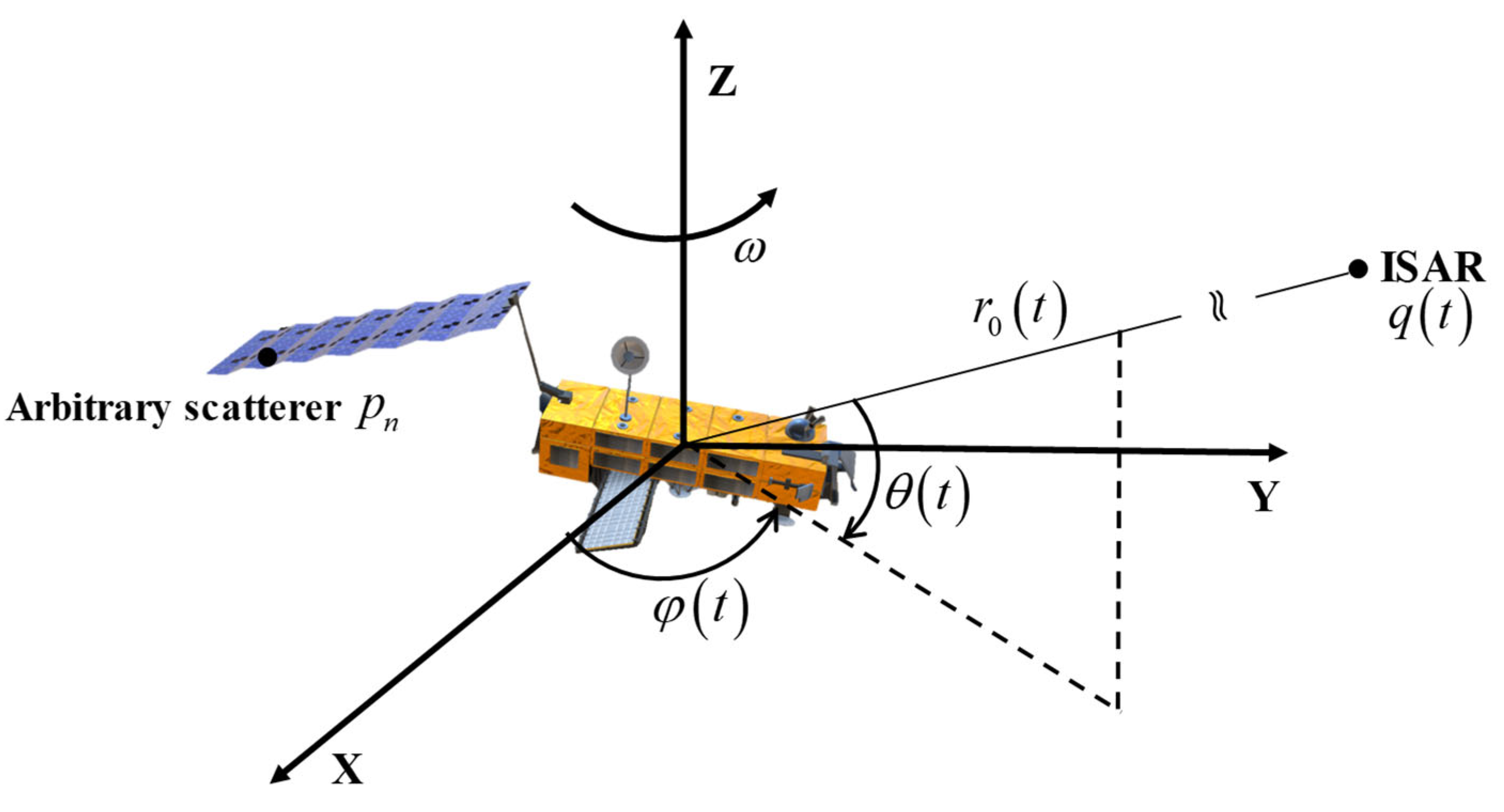
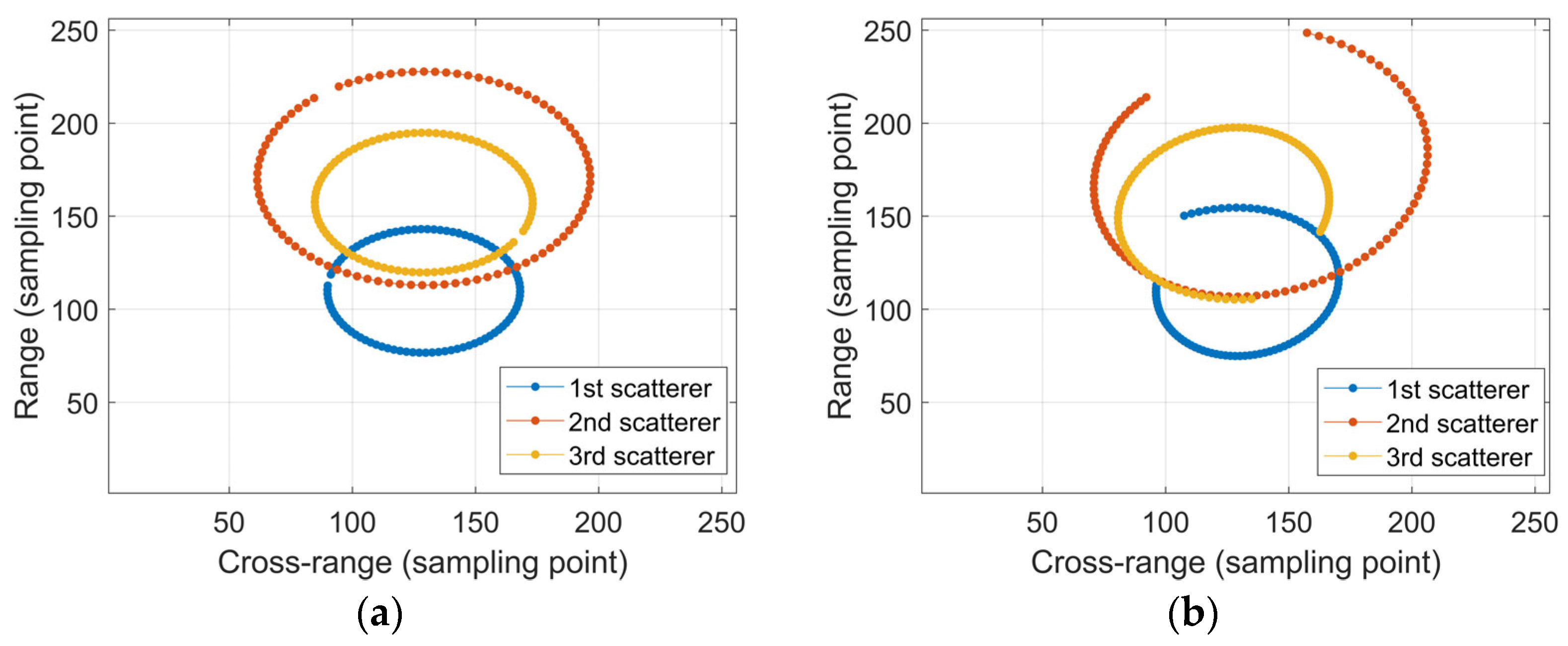
2. ISAR Imaging Model and Scatterer Trajectory Motion Characteristics Analysis

Taking a space target as an example, the ISAR observation model can be equated to the turntable model as shown in Figure 1 after the translational motion compensation. An ISAR image is the projection of the 3D geometry of the space target on the imaging plane. The range resolution of an ISAR image is dependent on the signal bandwidth of the transmitted electromagnetic wave. The larger the signal bandwidth is, the higher the range resolution is. The cross-range resolution of an ISAR image depends on the relative rotational angle of the target to the radar line of sight (LOS). The larger the relative rotational angle is, the smaller the wavelength of the transmitted electromagnetic wage is, and the higher the cross-range resolution. A simpler target observation model has been constructed in Refs. [11,13], where the motion of the observed target relative to the radar LOS during a single coherent processing interval (CPI) is approximated as if the radar LOS remains fixed while the observed target rotates around a specific axis. In Figure 1, the azimuth and pitch angles of the radar LOS vector are denoted by $\phi \left(t\right)$ and $\theta \left(t\right)$, respectively. The instantaneous radial distance and Doppler frequency of an arbitrary scatterer $p_n={\left[x_n,y_n,z_n\right]}^T$ can be represented by $r_n\left(t\right)$ and $f_n\left(t\right)$, respectively. Consequently, the projection positions of each scatterer adhere to certain relationships, which are as follows:

$$\left[\begin{array}{c}{r}_n\left(t\right)\\ {\displaystyle \frac{f_n\left(t\right)+z_n\sin \left(\theta \left(t\right)\right)}{\cos \left(\theta \left(t\right)\right)}}\end{array}\right]=\left[\begin{array}{cc}\sin \left(\omega t-\phi \left(t\right)\right)& \cos \left(\omega t-\phi \left(t\right)\right)\\ -\cos \left(\omega t-\phi \left(t\right)\right)& \sin \left(\omega t-\phi \left(t\right)\right)\end{array}\right]\times \left[\begin{array}{l}{x}_n\\ y_n\end{array}\right]$$

(1)

Figure 1. ISAR observation and imaging model.

It can be seen clearly from Equation (1) that the following equation holds:

$${\left(x_n\right)}^2+{\left(y_n\right)}^2={\left(d_n\right)}^2$$

(2)

where $d_n$ is the rotation radius of scatterer $p_n$ on the O-XY plane. Hence, we can obtain the following equation:

$${\displaystyle \frac{r_n^2\left(t\right)}{d_n^2}}+{\displaystyle \frac{{\left(f_n\left(t\right)+z_n\sin \theta \left(t\right)\right)}^2}{d_n^2{\cos }^2\theta \left(t\right)}}=1$$

(3)

It can be noted from Equation (3) that the scatterer trajectory of a space target with stationary motion will exhibit elliptical motion when the pitch angle of the LOS remains unchanged under the observation. Based on the above assumptions, Refs. [10,11] have proposed the scatterer trajectory association methods based on the improved MHT and MCMCDA algorithms, respectively. With the precise scatterer trajectory motion model, great performance can be achieved. However, the motion of a maneuvering space target may not coincide with the rotation around the fixed OZ axis in practical target observation scenarios, resulting in the equivalent radar LOS varying with the observation time. In other words, besides the rotation motion around the OZ axis, there exists additional rotation motion around an arbitrary axis for a maneuvering space target. Consequently, the short axis and the elliptic center described by Equation (3) will also change with time, forming an elliptic helix. In fact, the rotation motion of the space target around the OZ axis can be seen as the variation of the azimuth angle of the radar LOS. Hence, the motion of a maneuvering space target includes the following two parts: the variation of the azimuth angle of the radar LOS and the rotation motion around an arbitrary axis. To illustrate the differences between the scatterer trajectories of the space target with different motions, a simulation is performed as shown in Figure 2. In Figure 2a, the azimuth angle of the radar LOS varies with time, while the pitch angle of the radar LOS and the attitude of the space target remain unchanged. In Figure 2b, an additional rotation motion around an arbitrary axis is added for the space target compared with Figure 2a. It can be noted that the scatterer trajectories in Figure 2a coincide with elliptical motion while those in Figure 2b exhibit an elliptic helix, rendering the existing elliptic trajectory-based scatterer trajectory association methods inapplicable.

Figure 2. Illustration of scatterer trajectories on different imaging planes under fixed radar LOS and varied radar LOS, respectively. (a) Elliptical trajectories. (b) Non-elliptical trajectories.

To tackle this issue, a novel scatterer trajectory association method is proposed within the framework of RFS, which is independent of the elliptical trajectory model. The mathematical optimization model for the scatterer trajectory association will be established in the following section.

3. Optimization Model for Scatterer Trajectory Association Within the Framework of RFS

An RFS is characterized by a set whose elements and number of elements are both subject to randomness. Essentially, an RFS encapsulates a collection of random variables. Let $X_k=\left\{x_k^1,x_k^2,\dots ,x_k^N\right\}$ represent the state of the scatterers at the kth image frame, and the possible values of $X_k$ are as follows:

$$\begin{array}{l}\begin{array}{cc}{X}_k=\varnothing \hfill & \mathrm{when} \mathrm{no} \mathrm{scatterer} \mathrm{exists}\end{array}\\ \begin{array}{cc}{X}_k=\left\{x_k^1\right\}\hfill & \mathrm{when} \mathrm{one} \mathrm{scatterer} \mathrm{exists} \mathrm{and} \mathrm{its} \mathrm{state} \mathrm{is} x_k^1\end{array}\\ \begin{array}{cc}{X}_k=\left\{x_k^1,x_k^2\right\}\hfill & \mathrm{when} \mathrm{two} \mathrm{scatterers} \mathrm{exist} \mathrm{and} x_k^1\ne x_k^2\end{array}\\ \begin{array}{ccc}& ⋮& \end{array}\end{array}$$

(4)

where $x_k^i$ denotes the state of ith scatterer. Equation (4) illustrates that both the elements and the number of elements within an RFS are subject to randomness, and there are no identical elements within the set. Mahle proposed the PHD filtering algorithm in 2003 [23], which approximates an RFS as a Poisson RFS (PRFS). Specifically, the probability density function of a PRFS is given by the following form:

$$\lambda \left(x\right)=D\left(x\right)$$

(5)

where the following equation:

$$D\left(x\right)={\displaystyle \int p_X\left(X\right){\displaystyle \sum _{x^{\prime }\in X}\delta \left(x-x^{\prime }\right)\delta X}}$$

(6)

represents the PHD function of the RFS $X$, and $x$ is a variable of the PHD function.

The PHD function, as the first-order moment of the RFS, is also known as the intensity function of the RFS. Consequently, similar to Bayesian recursive filtering, the PHD filter’s task is to recursively determine the posteriori PHD of the scatterer state, given the motion and measurement models. This estimation process can be divided into the following two main steps [23]:

(1)

Prediction

$$\left\{\begin{array}{l}{D}_{k|k-1}\left(X_k|Z_{1:k-1}\right)={\displaystyle \int {\kappa }_{k|k-1}\left(X_k|X_{k-1}\right)D_{k|k-1}\left(X_{k-1}|Z_{1:k-1}\right)d{X}_{k-1}}+{\lambda }_{b,k}\left(X_k\right)\\ {\kappa }_{k|k-1}\left(X_k|X_{k-1}\right)=p_{s,k}\left(X_{k-1}\right)f\left(X_k|X_{k-1}\right)\end{array}\right.$$

(7)

where ${\lambda }_{b,k}\left(X_k\right)$ represents the PHD of newly born scatterers at the kth image frame, $p_{s,k}\left(X_{k-1}\right)$ denotes the survival probability of the scatterers, and $f\left(X_k|X_{k-1}\right)$ is the state transition function describing the evolution of scatterers from the (k − 1)th image frame.

(2)

Update

$$D_k\left(X_k|Z_{1:k}\right)={\vartheta }_{Z_k}\left(X_k\right)D_{k|k-1}\left(X_k|Z_{1:k-1}\right)$$

(8)

$$\begin{array}{c}{\vartheta }_{Z_k}\left(X_k\right)=1-p_{D,k}\left(X_k\right)\hfill \\ \hspace{1em}\hspace{1em}\hspace{1em} +p_{D,k}\left(X_k\right){\displaystyle \sum _{z\in Z_k}\frac{{\phi }_k\left(z|x_k\right)}{{\overline{\lambda }}_{c}c\left(z\right)+{\displaystyle \int p_{D,k}\left(X_k\right){\phi }_k\left(z|\zeta \right)}{D}_{k|k-1}\left(\zeta |Z_{1:k-1}\right)d\zeta }}\end{array}$$

(9)

where $p_{D,k}\left(X_k\right)$ represents the scatterer detection probability at the kth image frame, ${\overline{\lambda }}_c$ is the Poisson parameter, $c\left(z\right)$ denotes the clutter probability distribution, and ${\phi }_k\left(z|x_k\right)$ is the likelihood function of scatterer extraction.

It is evident from the PHD filtering process that the requirement for set integration computations restricts its application in practical scenarios. Although the computational burden has been lessened compared to the Bayesian iterative filter, this remains a challenge. Consequently, a series of related algorithms have been developed to address this issue, such as the Gaussian mixture PHD (GM-PHD) filter [26], the cardinalized probability hypothesis density (C-PHD) filter [27], and the particle probability hypothesis density (P-PHD) filter [28,29]. These algorithms have demonstrated their effectiveness in practical applications while preserving the superior performance characteristics of PHD filters. Inspired by these advancements, the GM-PHD filtering algorithm will be adapted to accommodate the specific features of the scatterer trajectory association problem.

4. Methodology

4.1. Modified Label Gaussian Mixture Probability Hypothesis Density Filter-Based Trajectory Association

The GM-PHD filter approximates the posteriori PHD as a weighted sum of multiple Gaussian distributions. This approach allows for obtaining a closed-form solution of the PHD filter under a linear Gaussian model, effectively circumventing the dimensionality challenges, often referred to as the ’curse of dimensionality’, associated with numerical integration in PHD filtering algorithms. However, the GM-PHD filter cannot be directly applied to the scatterer trajectory association problem. To address this, each Gaussian component within the GM-PHD filter is augmented with an independent label to associate the trajectory of each target [30]. Despite this modification, there remain the following three primary challenges associated with the label GM-PHD (L-GM-PHD) filter:

(1)

In practical scenarios, the prior PHD for a nascent target should be fixed in L-GM-PHD, which limits its practical application;

(2)

False alarms may persist even after pruning Gaussian components solely based on their weights;

(3)

The absence of an effective trajectory fusion strategy can lead to flawed trajectory associations.

In light of these challenges, a modified label Gaussian mixture probability hypothesis density filtering algorithm is proposed to associate the scattering center trajectories in ISAR image sequences, building upon the L-GM-PHD filter [31]. This algorithm enables the construction of a complete trajectory matrix and, subsequently, the application of factorization decomposition to achieve a 3D reconstruction of the observed target. The specific steps of the proposed algorithm are as follows:

(1)

Prediction

Assume that the PHD of the posterior distribution of the random finite set $p\left(X_{k-1}|Z_{1:k-1}\right)$ at the (k − 1)th image frame is as follows:

$$D_{k-1|k-1}\left(x\right)={\displaystyle \sum _{h=1}^{{\mathcal{H}}_{k-1|k-1}}{w}_{k-1|k-1}^h\mathcal{N}\left(x;{\mu }_{k-1|k-1}^h,P_{k-1|k-1}^h\right)}$$

(10)

where $x$ represents the scatterer state variable, and ${\mathcal{H}}_{k-1|k-1}$ denotes the number of Gaussian components in the posteriori PHD at the (k − 1)th image frame. In essence, the number of Gaussian components is equivalent to the number of scatterers. $w_{k-1|k-1}^h$, ${\mu }_{k-1|k-1}^h$ and $P_{k-1|k-1}^h$ denote the weight, mean vector, and variance matrix of the hth Gaussian component, respectively. It is important to note that since the PHD is not a probability density function, the sum of the weights does not equal 1. Given that each Gaussian component in Equation (10) corresponds to the state of each scattering center at the kth image frame, an identifiable label is assigned to each Gaussian component. This labeling process is crucial for discriminating between the scattering centers.

$$L_{k-1}=\left\{l_{k-1}^1,\dots ,l_{k-1}^{{\mathcal{H}}_{k-1|k-1}}\right\}$$

(11)

To effectively identify the starting point of a scatterer trajectory, the PHD of a newly detected scatterer trajectory can be modeled as a mixture of Gaussian distributions that encompasses all the measurements within that particular image frame. Concurrently, the PHD is updated in tandem with the iterative process. Thus, the PHD of a newly detected scatterer trajectory can be expressed as follows:

$${\lambda }_{b,k}\left(x\right)={\displaystyle \sum _{h=1}^{{\mathcal{H}}_k^b}{w}_{b,k}^h\mathcal{N}\left(x;{\mu }_{b,k}^h,P_{b,k}^h\right)}$$

(12)

where ${\mathcal{H}}_k^b$, $w_{b,k}^h$, ${\mu }_{b,k}^h$ and $P_{b,k}^h$ denote the number, weight, mean vector, and variance matrix of the newly identified scatterers at the kth image frame, respectively. Clearly, $w_{b,k}^h={\displaystyle \frac{1}{{\mathcal{H}}_k^b}}$ and ${\mu }_{b,k}^h=z_k^h$, where $z_k^h\in Z_k$ is the hth measured position at the kth image frame.

For each newly identified scatterer, its Gaussian components should be assigned new and independent labels, which are shown as follows:

$$L_{b,k}=\left\{l_k^{{\mathcal{H}}_{k-1|k-1}+1},\dots ,l_k^{{\mathcal{H}}_{k-1|k-1}+{\mathcal{H}}_k^b}\right\}$$

(13)

Equation (13) reveals that the motion of each scattering center on the ISAR imaging plane follows a quasi-sinusoidal pattern. Consequently, the velocity and acceleration of these scattering centers also exhibit quasi-sinusoidal behavior, demonstrating strong maneuverability. For highly maneuverable targets, Ref. [32] proposed a ‘current’ motion model that captures this behavior, which can be expressed as follows:

$$x_{k+1}=F_k{x}_k+A_k{G}_k+w_k$$

(14)

where $x_{k+1}$ and $x_k$ represent the state variables of the scatterer at the (k + 1)th and kth image frames, respectively. $F_k$, $G_k$ and $w_k$ denote the scatterer motion state transition matrix, control matrix, and process noise matrix, respectively. The term $A_k$ represents the average acceleration matrix of the scatterer’s Doppler and radial distance. Therefore, the detailed expression of the scatterer state at the kth image frame is given by the following:

$$x_k={\left[f_n^k,v_{f,n}^k,a_{f,n}^k,r_n^k,v_{r,n}^k,a_{r,n}^k\right]}^T$$

(15)

The aforementioned equation encompasses the two-dimensional positions of the scattering center within the ISAR image, along with the velocity $\left(v_{f,n}^k,v_{r,n}^k\right)$ and acceleration $\left(a_{f,n}^k,a_{r,n}^k\right)$ of the scattering center in the rang dimension and cross-range dimension, respectively. To simplify the analysis, it is assumed that the position variations in the range and cross-range (Doppler) dimensions are independent. Consequently, as analyzed in Ref. [32], the state transition matrix is given by the following equation:

$$F_k=\left[\begin{array}{cccccc}1& \Delta t& \left({\alpha }_f\Delta t-1+e^{-{\alpha }_f\Delta t}\right)/{\alpha }_f^2& 0& 0& 0\\ 0& 1& \left(1-e^{-{\alpha }_f\Delta t}\right)/{\alpha }_f& 0& 0& 0\\ 0& 0& -e^{-{\alpha }_f\Delta t}& 0& 0& 0\\ 0& 0& 0& 1& \Delta t& \left({\alpha }_r\Delta t-1+e^{-{\alpha }_r\Delta t}\right)/{\alpha }_r^2\\ 0& 0& 0& 0& 1& \left(1-e^{-{\alpha }_r\Delta t}\right)/{\alpha }_r\\ 0& 0& 0& 0& 0& -e^{-{\alpha }_r\Delta t}\end{array}\right]$$

(16)

where $\Delta t$ represents the observation time interval between adjacent image frames. ${\alpha }_f$ and ${\alpha }_r$ denote the predetermined acceleration parameters of the scattering center in cross-range and range dimensions, respectively. The control input matrix is as follows:

$$\begin{array}{c}{G}_k=\left[\left(-\Delta t+{\displaystyle \frac{{\alpha }_f\Delta t^2}{2}}+{\displaystyle \frac{1-e^{-{\alpha }_f\Delta t}}{{\alpha }_f}}\right)/{\alpha }_f,\Delta t-\left(1-e^{-{\alpha }_f\Delta t}\right)/{\alpha }_f,1-e^{-{\alpha }_f\Delta t},\right.\\ {\left.\left(-\Delta t+{\displaystyle \frac{{\alpha }_r\Delta t^2}{2}}+{\displaystyle \frac{1-e^{-{\alpha }_r\Delta t}}{{\alpha }_r}}\right)/{\alpha }_r,\Delta t-\left(1-e^{-{\alpha }_r\Delta t}\right)/{\alpha }_r,1-e^{-{\alpha }_r\Delta t}\right]}^T\end{array}$$

(17)

The matrix $A_k$ is a diagonal matrix and its expression is shown as follows:

$$A_k=diag\left\{\left[{\overline{a}}_f^k,{\overline{a}}_f^k,{\overline{a}}_f^k,{\overline{a}}_r^k,{\overline{a}}_r^k,{\overline{a}}_r^k\right]\right\}$$

(18)

where ${\overline{a}}_f^k$ and ${\overline{a}}_r^k$ represent the average values of the position variation accelerations of the Doppler and the radial distance of the scattering center, respectively. In practice, these average values can be replaced by the predicted accelerations, that is as follows:

$$\left\{\begin{array}{l}{\overline{a}}_f^k=a_{f,n}^{k|k-1}\\ {\overline{a}}_r^k=a_{r,n}^{k|k-1}\end{array}\right.$$

(19)

Since it is assumed that the Doppler variation and the radial distance variation of the scattering center are independent, the noise covariance matrix $w_k$ of the state transition process can be expressed as follows:

$$Q_k=\left[\begin{array}{cc}{Q}_k^f& 0\\ 0& Q_k^r\end{array}\right]$$

(20)

where $Q_k^f\in {ℝ}^{3\times 3}$ and $Q_k^r\in {ℝ}^{3\times 3}$ denote the noise covariance matrices of the Doppler state transition process and radial distance state transition process of the scattering center, respectively. The expression of $Q_k^f$ is presented as follows:

$$Q_k^f=2{\alpha }_f{\sigma }_a^2\left[\begin{array}{ccc}{q}_{11}& q_{12}& q_{13}\\ q_{12}& q_{22}& q_{23}\\ q_{13}& q_{23}& q_{33}\end{array}\right]$$

(21)

where

$$\left\{\begin{array}{l}{q}_{11}={\displaystyle \frac{1}{2{\alpha }_f^5}}\left(1-e^{-2{\alpha }_f\Delta t}+2{\alpha }_f\Delta t+{\displaystyle \frac{2{\alpha }_f^3\Delta t^3}{3}}-2{\alpha }_f^2\Delta t^2-4\alpha \Delta t{e}^{-{\alpha }_f\Delta t}\right)\\ q_{12}={\displaystyle \frac{1}{2{\alpha }_f^4}}\left(1+e^{-2{\alpha }_f\Delta t}-2e^{-{\alpha }_f\Delta t}+2{\alpha }_f\Delta t{e}^{-{\alpha }_f\Delta t}-2{\alpha }_f\Delta t+{\alpha }_f^2\Delta t^2\right)\\ q_{13}={\displaystyle \frac{1}{2{\alpha }_f^3}}\left(1-e^{-2{\alpha }_f\Delta t}-2{\alpha }_f\Delta t{e}^{-{\alpha }_f\Delta t}\right)\\ q_{22}={\displaystyle \frac{1}{2{\alpha }_f^3}}\left(4e^{-{\alpha }_f\Delta t}-3-e^{-2{\alpha }_f\Delta t}+2{\alpha }_f\Delta t\right)\\ q_{23}={\displaystyle \frac{1}{2{\alpha }_f^2}}\left(e^{-2{\alpha }_f\Delta t}+1-2e^{-{\alpha }_f\Delta t}\right)\\ q_{33}={\displaystyle \frac{1}{2{\alpha }_f}}\left(1-e^{-2{\alpha }_f\Delta t}\right)\end{array}\right.$$

(22)

and

$${\sigma }_a^2={\displaystyle \frac{4-\pi }{\pi }}{\left(a_{\max }-{\overline{a}}_f^k\right)}^2$$

(23)

The representation of $Q_k^r$ can be derived by substituting ${\alpha }_f$ and ${\overline{a}}_f^k$ by ${\alpha }_r$ and ${\overline{a}}_r^k$, respectively. The current motion model for the scattering center is capable of modeling the position variance ${\sigma }_a^2$ of the Doppler and radial distance with high precision. This is attributed to its adaptive adjustment of the acceleration deviations of the Doppler and radial distance variations during the tracking process. Consequently, this model allows for the precise tracking of highly maneuverable targets.

Drawing on the Doppler and radial distance variation models for each scatterer, the transition model for the scattering center trajectory association state can be formulated as follows:

$${\pi }_k\left(X_k|\left\{x_{k-1}\right\}\right)=\left\{\begin{array}{cc}\begin{array}{l}1-P^S\\ P^S\mathcal{N}\left(x_k;F_{k-1}{x}_{k-1}+A_{k-1}{G}_{k-1},Q_{k-1}\right)\end{array}& \begin{array}{l}{X}_k=\varnothing \\ X_k=\left\{x_k\right\}\end{array}\end{array}\right.$$

(24)

where ${\pi }_k\left(X_k|\left\{x_{k-1}\right\}\right)$ denotes the PHD of the surviving scattering centers from the (k − 1)th image frame to the kth image frame. $P^S$ represents the survival probability. The definitions of $F_{k-1}$, $A_{k-1}$, $G_{k-1}$ and $Q_{k-1}$ can be found in the previous description and will not be explained here.

Furthermore, the random finite set of scattering centers at the kth image frame is considered the union of the random finite sets of surviving scattering centers from the (k − 1)th image frame and the newly born scattering centers at the kth image frame. Utilizing the summation property of the PHD, the predicted random finite set is a PRFS with an PHD given by the following equation:

$$D_{k|k-1}\left(x\right)=D_{k|k-1}^S\left(x\right)+{\lambda }_{b,k}\left(x\right)$$

(25)

where ${\lambda }_{b,k}\left(x\right)$ represents the PHD of the newly born scattering centers, conforming to a Gaussian mixture distribution. $D_{k|k-1}^S\left(x\right)$ denotes the summation of multiple single-scatterer Gaussian distributions, which can also be modeled as a Gaussian mixture distribution. The corresponding parameters for this distribution are presented as follows:

$$\begin{array}{l}{\mathcal{H}}_{k|k-1}^S={\mathcal{H}}_{k-1|k-1}\\ w_{k|k-1}^{s,h}=P^S{w}_{k-1|k-1}^h\\ {\mu }_{k|k-1}^{s,h}=F_{k-1}{\mu }_{k-1|k-1}^h+A_{k-1}{G}_{k-1}\\ P_{k|k-1}^{s,h}=F_{k-1}{P}_{k-1|k-1}^{s,h}{F}_{k-1}^T+Q_{k-1}\end{array}$$

(26)

As the state of each scattering center is updated during the prediction process, the label of each Gaussian component in the predicted PHD at the current image frame remains consistent with that of the posterior distribution at the previous image frame, as expressed in the following equation:

$$L_{k|k-1}=L_{k-1}\cup L_{b,k}$$

(27)

Consequently, the process of generating the predicted PHD is concluded in Algorithm 1, shown as follows:

Algorithm 1. Prediction Procedure of ML-GM-PHD Filtering Algorithm.

Input: ${\mu }_{k-1|k-1}^h$ and $P_{k-1|k-1}^h$ with $h$ ranging from 1 to ${\mathcal{H}}_{k-1|k-1}$, $w_{b,k}^h$, ${\mu }_{b,k}^h$ and $P_{b,k}^h$ with $h$ ranging from 1 to ${\mathcal{H}}_k^b$, $L_{b,k}$, $L_{k-1}$, $F_{k-1}$ and $Q_{k-1}$ 1: Set the number of the Gaussian components of the prediction PHD with ${\mathcal{H}}_{k|k-1}={\mathcal{H}}_k^b+{\mathcal{H}}_{k-1|k-1}$ 2: For $h=1:{\mathcal{H}}_k^b$ 3:    $\begin{array}{cccc}{w}_{k|k-1}^h=w_{b,k}^h,& {\mu }_{k|k-1}^h={\mu }_{b,k}^h,& P_{k|k-1}^h=P_{b,k}^h,& L_{b,k|k-1}=L_{b,k}\end{array}$ 4: End for 5: For $h=1:{\mathcal{H}}_{k-1|k-1}$ 6:    $\begin{array}{ccc}{w}_{k|k-1}^{h+{\mathcal{H}}_k^b}=P^S{w}_{b,k}^h,& {\mu }_{k|k-1}^{h+{\mathcal{H}}_k^b}=F_{k-1}{\mu }_{k-1|k-1}^h+A_{k-1}{G}_{k-1},& P_{k|k-1}^{h+{\mathcal{H}}_k^b}=F_{k-1}{P}_{k-1|k-1}^h{F}_{k-1}^T+Q_{k-1},\end{array}{L}_{k|k-1}=L_{k-1}$

7: End for Output: $w_{k|k-1}^h$, ${\mu }_{k|k-1}^h$, $P_{k|k-1}^h$, $L_{k|k-1}^h$ with $h$ ranging from 1 to ${\mathcal{H}}_{k|k-1}$

(2)

Update

If the posterior PHD of the scatterer centers at the (k − 1)th image frame is a PRFS, then the prediction distribution will also be a PRFS. Consequently, the prediction PHD, as presented in Equations (25) and (26), can be expressed in the following form:

$$D_{k|k-1}\left(x\right)={\displaystyle \sum _{h=1}^{{\mathcal{H}}_{k|k-1}}{w}_{k|k-1}^h\mathcal{N}\left(x;{\mu }_{k|k-1}^h,P_{k|k-1}^h\right)}$$

(28)

It can be assumed that the standard measurement model of each scatterer center is a Bernoulli random finite set, as in the following equation:

$$g_k\left(Z_k|\left\{x_k\right\}\right)=\left\{\begin{array}{cc}\begin{array}{l}1-P^D\\ P^D\mathcal{N}\left(z_k;H_k{x}_k,R_k\right)\\ 0\end{array}& \begin{array}{l}{Z}_k=\varnothing \\ Z_k=\left\{z_k\right\}\\ \left|Z_k\right|>1\end{array}\end{array}\right.$$

(29)

where the detection probability $P^D$ is a constant, the probability density function $g_k$ is a Gaussian distribution, $H_k$ denotes the measurement matrix, and $R_k$ represents the covariance matrix of the measurement noise. Since the measurement values are the projected radial distance and Doppler frequency of the scattering center, the measurement matrix can be formulated as follows:

$$H_k=\left[\begin{array}{cccccc}1& 0& 0& 0& 0& 0\\ 0& 0& 0& 1& 0& 0\end{array}\right]$$

(30)

The posterior distribution $P\left(X_k|Z_{1:k}\right)$ is a Poisson multi-Bernoulli randomized finite set (PMBRFS), where the PHD of a PRFS is as follows:

$${\lambda }_{k|k}\left(x\right)=\left(1-P^D\right)D_{k|k-1}\left(x\right)$$

(31)

Equation (31) represents the PHD of scattering centers that are not associated with any measurements, implying that these originate entirely from the clutter. By substituting Equation (28) into Equation (31), we can derive the following result:

$${\lambda }_{k|k}\left(x\right)={\displaystyle \sum _{h=1}^{{\mathcal{H}}_{k|k-1}}\left(1-P^D\right)w_{k|k-1}^h\mathcal{N}\left(x;{\mu }_{k|k-1}^h,P_{k|k-1}^h\right)}$$

(32)

Consequently, the scattering centers depicted in Equation (32) can be regarded as the preceding Gaussian components of the posterior PHD of the scattering centers. Furthermore, the posterior PHD encompasses $m_k$ Bernoulli random finite sets, with its PHD given by the following:

$$D_{k|k}^o\left(x\right)={\displaystyle \sum _{i=1}^{m_k}{r}_{k|k}^i{p}_{k|k}^i\left(x\right)}$$

(33)

where

$$\begin{array}{l}{r}_{k|k}^i={\displaystyle \frac{P^D{\displaystyle \int \mathcal{N}\left(z_k^i;H_k{x}^{\prime },R_k\right)D_{k|k-1}\left(x^{\prime }\right)}d{x}^{\prime }}{{\lambda }_c\left(z_k^i\right)+P^D{\displaystyle \int \mathcal{N}\left(z_k^i;H_k\tilde{x},R_k\right)D_{k|k-1}\left(\tilde{x}\right)}d\tilde{x}}}\\ p_{k|k}^i\left(x\right)\propto \mathcal{N}\left(z_k^i;H_{k}x,R_k\right)D_{k|k-1}\left(x\right)\end{array}$$

(34)

Following approximation by a PRFS, the posterior PHD can be expressed as follows:

$$r_{k|k}^i{p}_{k|k}^i\left(x\right)={\displaystyle \sum _{h=1}^{{\mathcal{H}}_{k|k-1}}\left(1-P^D\right)w_k^{h,i}\mathcal{N}\left(x;{\mu }_k^{h,i},P_k^{h,i}\right)}$$

(35)

where

$$\mathcal{N}\left(x;{\mu }_k^{h,i},P_k^{h,i}\right)\propto \mathcal{N}\left(z_k^i;H_{k}x,R_k\right)\mathcal{N}\left(x;{\mu }_{k|k-1}^h,P_{k|k-1}^h\right)$$

(36)

Therefore, based on the measurement model, $\mathcal{N}\left(z_k^i;H_{k}x,R_k\right)$, $\mathcal{N}\left(x;{\mu }_k^{h,i},P_k^{h,i}\right)$ can be updated from $\mathcal{N}\left(x;{\mu }_{k|k-1}^h,P_{k|k-1}^h\right)$ using the Kalman filtering. Since the measurement model $\mathcal{N}\left(z_k^i;H_{k}x,R_k\right)$ is independent of the scattering center index $i$, that is, each scattering center adheres to the same measurement model, it is reasonable to update each Gaussian component corresponding to index $h$ individually.

Regarding the update process for each Gaussian component, there exist $\left(m_k+1\right)$ potential scenarios; the prediction could originate from the ith observation or from the Gaussian noise. Consequently, a total of $\left(m_k+1\right)$ prediction components will share the same labels.

The above description outlines the update process for the PHD of scattering centers, and the specific algorithm can be encapsulated as shown in Algorithm 2:

Algorithm 2. Update Process of ML-GM-PHD Filtering Algorithm.

Input: $w_{k|k-1}^h$, ${\mu }_{k|k-1}^h$, $P_{k|k-1}^h$, $L_{k|k-1}^h$ with $h$ ranging from 1 to ${\mathcal{H}}_{k|k-1}$, $P^D$, $H_k$ and $R_k$ 1: For $h=1:{\mathcal{H}}_{k|k-1}$ let 2:    $\begin{array}{cccc}{w}_{k|k}^h=\left(1-P^D\right)w_{k|k-1}^h,& {\mu }_{k|k}^h={\mu }_{k|k-1}^h,& P_{k|k}^h=P_{k|k-1}^h,& L_{k|k}^h=L_{k|k-1}^h\end{array}$ 3: End for 4: For $h=1:{\mathcal{H}}_{k|k-1}$ let 5:   ${\widehat{z}}_{k|k-1}^h=H_k{\mu }_{k|k-1}^h$ 6:   $S_k^h=H_k{P}_{k|k-1}^h{H}_k^T+R_k$ 7:   $K_k^h=P_{k|k-1}^h{H}_k^T{\left(S_k^h\right)}^{-1}$ 8:   $P_k^h=\left(I-K_k^h{H}_k\right)P_{k|k-1}^h$ 9: End for 10: For $h=1:m_k$ 11:    for $h=1:{\mathcal{H}}_{k|k-1}$ let 12:      ${\mu }_{k|k}^{i{\mathcal{H}}_{k|k-1}+h}={\mu }_{k|k-1}^h+K_h^h\left(z_k^i-{\widehat{z}}_{k|k-1}^h\right)$ 13:      $P_{k|k}^{i{\mathcal{H}}_{k|k-1}+h}=P_k^h$ 14:      ${\tilde{w}}_{k|k}^{i{\mathcal{H}}_{k|k-1}+h}=P^D{w}_{k|k-1}^h\mathcal{N}\left(z_k^i;{\widehat{z}}_{k|k-1}^h,S_k^h\right)$ 15:      $L_{k|k}^{i{\mathcal{H}}_{k|k-1}+h}=L_{k|k-1}^h$ 16:    end for 17:    for $h=1:{\mathcal{H}}_{k|k-1}$ let 18:    $w_{k|k}^{i{\mathcal{H}}_{k|k-1}+h}={\displaystyle \frac{{\tilde{w}}_{k|k}^{i{\mathcal{H}}_{k|k-1}+h}}{{\lambda }_c\left(z_k^i\right)+{\displaystyle \sum _{h\prime =1}^{{\mathcal{H}}_{k|k-1}}{\tilde{w}}_{k|k}^{i{\mathcal{H}}_{k|k-1}+h\prime }}}}$ 19:    end for 20: End for Output: $w_{k|k}^h$, ${\mu }_{k|k}^h$, $P_{k|k}^h$ and $L_{k|k}^h$ with $h$ ranging from 1 to $\left(m_k+1\right)\times {\mathcal{H}}_{k|k-1}$

(3)

Prune and merge

During the iterative filtering process, each corresponding case of the scattering center state and the measurements is considered, leading to the accumulation of a large number of Gaussian mixing terms in both the prediction and updating stages. The variation in the number of Gaussian mixing terms is governed by the following equation:

$$\begin{array}{l}{\mathcal{H}}_{k|k-1}={\mathcal{H}}_{k-1|k-1}+{\mathcal{H}}_k^b\\ {\mathcal{H}}_{k|k}=\left(m_k+1\right)\times {\mathcal{H}}_{k|k-1}\end{array}$$

(37)

In the prediction process, the Gaussian mixing terms encompass those that are carried over from the previous iteration as well as newly generated terms. During the update phase, each filtered result includes $\left(m_k+1\right)$ predicted Gaussian mixed terms.

Consequently, after the update process, a multitude of interfering Gaussian components are present. Notably, there may be multiple Gaussian components associated with the same scatterer state. Therefore, it becomes essential to reorganize the labels of all Gaussian components. This involves pruning the Gaussian components that correspond to false scattering centers and merging those that represent the same scattering center state. Given that the PHD of a newly born scattering center is constructed from measurement data, clutter far from the potential scattering center region cannot be solely pruned based on weights. Hence, both the weight coefficients and the spatial distribution of the Gaussian components are employed as criteria for pruning. Gaussian terms with weight coefficients below a predetermined threshold or with spatial distributions outside the scatterer areas will be pruned. Simultaneously, multiple Gaussian components exhibiting similar spatial distributions will be consolidated into a single component, with its weight set to the sum of the weights of the individual Gaussian components.

(4)

Scatterer state extraction

After pruning and merging, the interfering Gaussian components are effectively mitigated. Consequently, by extracting the Gaussian components with the largest ${\widehat{\mathcal{H}}}_{k|k}$ weights from the posterior PHD, the PHD of the scatterers at the kth image frame can be determined. Subsequently, the state of each scatterer can be derived by calculating the mean value of each corresponding PHD. The effective Gaussian distribution after extraction is assumed to be as follows:

$$D_{k|k}\left(x\right)={\displaystyle \sum _{h=1}^{{\widehat{\mathcal{H}}}_{k|k}}{w}_{k|k}^h\mathcal{N}\left(x;{\mu }_{k|k}^h,P_{k|k}^h\right)}$$

(38)

To proceed with the subsequent iteration of the solution, it is necessary to update the PHD of the newly born scattering centers as follows:

$${\lambda }_{b,k+1}\left(x\right)=D_{k|k}\left(x\right)+{\displaystyle \sum _{h=1}^{{\mathcal{H}}_{k+1}^o}\frac{1}{{\mathcal{H}}_{k+1}^o}\mathcal{N}\left(x;{\mu }_{o,k+1}^h,P_{o,k+1}^h\right)}$$

(39)

where ${\mu }_{o,k+1}^h=z_{k+1}^h$, $z_{k+1}^h\in Z_{k+1}$ represent the hth measurement value at the (k + 1)th image frame. The PHD at the kth image frame and the measurement PHD at the (k + 1)th image frame are both used as the intensity function of the newly born scattering centers. This algorithm ensures robust detection and tracking of the scattering centers.

4.2. Trajectory Integration and Management

Upon completion of the recursive filtering process within the PHD framework, the majority of scattering centers in the ISAR image sequence are able to form a complete trajectory. However, due to the presence of clutter and missed detections, the trajectories of certain scattering centers may not be confirmed at the beginning but will be recognized as real trajectories after a period of recursive filtering. Concurrently, there may be incomplete trajectories induced by a long time of leakage detection. To address these challenges, target trajectories are associated in two complementary directions, as referenced in Ref. [10]. Initially, the ML-GM-PHD filtering algorithm is applied along the forward image frame sequence. Subsequently, the trajectories are associated in the reverse direction by employing the proposed algorithm. The final step involves merging the trajectories obtained from both the forward and reverse directions, thereby enhancing the overall performance of the proposed algorithm.

During the PHD-based recursive filtering process, the algorithm will record the image frame $k$ and the label $L_k^i$ of each identified scattering center. Therefore, by comparing the state of each scattering center at the same image frame, the scatterer state can be merged to obtain a complete trajectory. Assuming that trajectories of the ith scattering center obtained from both the forward association and backward association can be represented as follows:

$$\begin{array}{l}{\mathcal{T}}^{positive,i}=\left\{x_1^{positive,i},x_2^{positive,i},\dots ,x_K^{positive,i}\right\}\\ {\mathcal{T}}^{negative,i}=\left\{x_1^{negative,i},x_2^{negative,i},\dots ,x_K^{negative,i}\right\}\end{array}$$

(40)

where $x_k^{positive,i}$ and $x_k^{negative,i}\left(k=1,2,\dots ,K\right)$ may be $\varnothing$.

Hence, the proposed fusion strategy is presented as follows. If there exists only one trajectory point for ith scatterer at the kth image frame corresponding to the forward or backward association, i.e., $x_k^{negative,i}=\varnothing$ or $x_k^{positive,i}=\varnothing$, then this trajectory point will be seen as the fused trajectory point of ith scatterer at the current moment. If not, the average of the points from both the forward trajectory and backward trajectory will be employed as the fused trajectory point for the current moment. The fusion strategy can be described in the following equation:

$$x_k^{fusion,i}=\left\{\begin{array}{cc}{x}_k^{positive,i}& x_k^{negative,i}=\varnothing \\ x_k^{negative,i}& x_k^{positive,i}=\varnothing \\ {\displaystyle \frac{x_k^{positive,i}+x_k^{negative,i}}{2}}& x_k^{positive,i},x_k^{positive,i}\ne \varnothing \end{array}\right.$$

(41)

Furthermore, there are instances where trajectory points are absent due to leakage detection. Utilizing the proposed ML-GM-PHD filtering algorithm, the missing scatterer states can be effectively predicted based on the existing filtered trajectory points.

$$\begin{array}{l}{\widehat{x}}_k^{positive,i}={\left[{\stackrel{⌢}{f}}_k^{positive,i},{\widehat{v}}_{f,k}^{positive,i},{\widehat{a}}_{f,k}^{positive,i},{\widehat{r}}_k^{positive,i},{\widehat{v}}_{r,k}^{positive,i},{\widehat{a}}_{r,k}^{positive,i}\right]}^T\\ {\widehat{x}}_k^{negative,i}={\left[{\stackrel{⌢}{f}}_k^{negative,i},{\widehat{v}}_{f,k}^{negative,i},{\widehat{a}}_{f,k}^{negative,i},{\widehat{r}}_k^{negative,i},{\widehat{v}}_{r,k}^{negative,i},{\widehat{a}}_{r,k}^{negative,i}\right]}^T\end{array}$$

(42)

Assuming that there exists a missing point at the $k_m$th image frame, the position of this point can be estimated by predicting the scatterer state based on the states of adjacent image frames. If ${\widehat{x}}_{k_m-1}^{positive,i}$ and ${\widehat{x}}_{k_m+1}^{negative,i}$ exist, the scatterer position at the $k_m$th image frame can be predicted by the following equations:

$$\begin{array}{l}{\stackrel{⌢}{f}}_{k_m}^{positive,i}={\displaystyle \frac{{\stackrel{⌢}{f}}_{k_m-1}^{positive,i}+{\stackrel{⌢}{f}}_{k_m+1}^{negative,i}+\left({\widehat{v}}_{f,k_m-1}^{positive,i}+{\widehat{v}}_{f,k_m+1}^{negative,i}\right)\Delta t+\frac{1}{2}\left({\widehat{a}}_{f,k_m-1}^{positive,i}+{\widehat{a}}_{f,k_m+1}^{negative,i}\right)\Delta t^2}{2}}\\ {\widehat{r}}_{k_m}^{positive,i}={\displaystyle \frac{{\widehat{r}}_{k_m-1}^{positive,i}+{\widehat{r}}_{k_m+1}^{negative,i}+\left({\widehat{v}}_{r,k_m-1}^{positive,i}+{\widehat{v}}_{r,k_m+1}^{negative,i}\right)\Delta t+\frac{1}{2}\left({\widehat{a}}_{r,k_m-1}^{positive,i}+{\widehat{a}}_{r,k_m+1}^{negative,i}\right)\Delta t^2}{2}}\end{array}$$

(43)

If neither ${\widehat{x}}_{k_m-1}^{positive,i}$ nor ${\widehat{x}}_{k_m+1}^{negative,i}$ exists, the scatterer state can be estimated by a one-step prediction of ${\widehat{x}}_{k_m+1}^{positive,i}$ or ${\widehat{x}}_{k_m-1}^{negative,i}$. Moreover, when the number of missing points exceeds one, scatterer positions can be estimated through multi-step prediction. However, the prediction is generally most effective when the number of missing points does not exceed three.

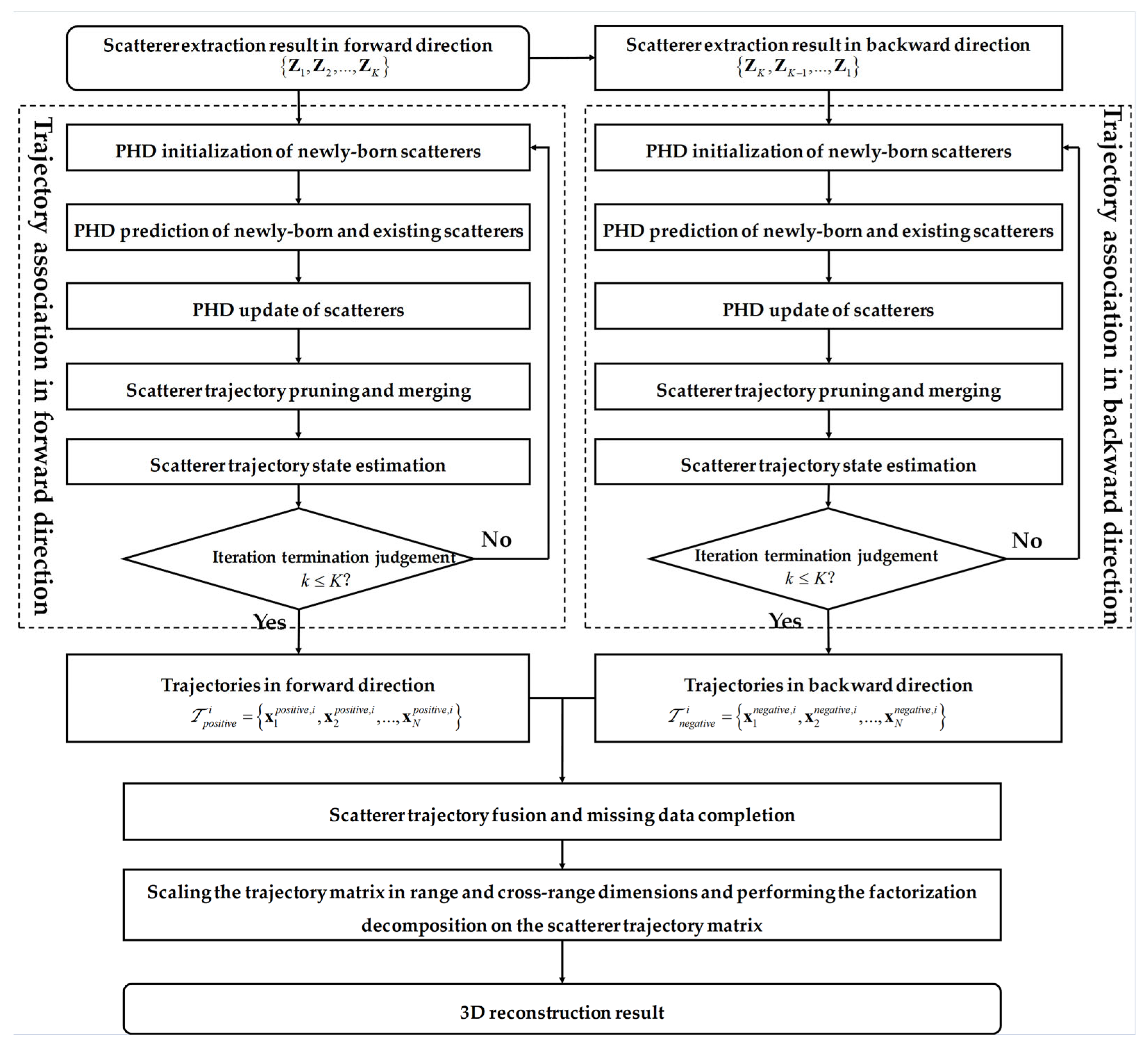
4.3. Algorithm Summation

In conclusion, complete trajectories of the scattering centers in the ISAR image sequence can be obtained by the proposed ML-GM-PHD filtering algorithm. After the trajectory association processing, the complete trajectory of ith scattering center can be rewritten as follows:

$${\mathcal{T}}_{complete}^i=\left\{x_1^{complete,i},x_2^{complete,i},\dots ,x_K^{complete,i}\right\},i=1,2,\dots ,N$$

(44)

The scatterer trajectory matrix of the space target can be constructed by rewriting each scattering trajectory into a matrix form such as the following:

$$W=\left[{\displaystyle \frac{U}{V}}\right]=\left[\begin{array}{ccc}{f}_{11}& \cdots & f_{1N}\\ ⋮& \ddots & ⋮\\ f_{K1}& \cdots & f_{KN}\\ r_{11}& \cdots & r_{1N}\\ ⋮& \ddots & ⋮\\ r_{K1}& \cdots & r_{KN}\end{array}\right]$$

(45)

where $U$ and $V$ denotes the Doppler trajectory sub-matrix and slant-range trajectory sub-matrix of scattering centers, respectively.

However, since the trajectory matrix is based on the image pixel values, the 3D geometry obtained directly from the factorization decomposition of this matrix will exhibit geometric distortion. To address this, it is essential to perform a two-dimensional scale calibration on the associated trajectory matrix. This involves multiplying the range pixel coordinates by the range resolution unit ${\rho }_r$ and multiplying the cross-range pixel coordinates by the cross-range resolution unit ${\rho }_a$, respectively. The ${\rho }_r$ can be calculated using the signal bandwidth and sampling frequency of the ISAR system, while the ${\rho }_a$ is determined by the equivalent rotational angular velocity of the target. Detailed estimation algorithms for these parameters are discussed in Refs. [33,34], which will not be reiterated here. Ultimately, the factorization decomposition of the calibrated trajectory matrix is applied to obtain the target 3D scattering center coordinates [14]. Figure 3 illustrates the specific flowchart of the proposed algorithm.

Figure 3. Flowchart of ML-GM-PHD filtering-based scatterer trajectory association and 3D reconstruction algorithm.

As presented in Figure 3, the flowchart of the proposed algorithm is presented as follows:

Step (1):

Input the scatterer extraction results of the image sequence in forward and backward directions.

Step (2):

Performing the ML-GM-PHD filtering processing along the forward and backward directions, respectively. In the ML-GM-PHD filtering processing, PHD initialization of newly born scatterers, PHD prediction, PHD update, scatterer trajectory pruning and merging, scatterer trajectory state estimation are sequentially performed on the input scatterer extraction results. Associated trajectories in forward direction and backward direction can be obtained after the iteration processing.

Step (3):

Performing the scatterer trajectory fusion processing and estimating the missing points. Consequently, complete scatterer trajectory matrix is obtained.

Step (4):

Scaling the scatterer trajectory matrix in range dimension and cross-range dimension.

Step (5):

Performing the factorization decomposition on the scatterer trajectory matrix to obtain the 3D reconstruction result.

5. Experimental Results and Analysis

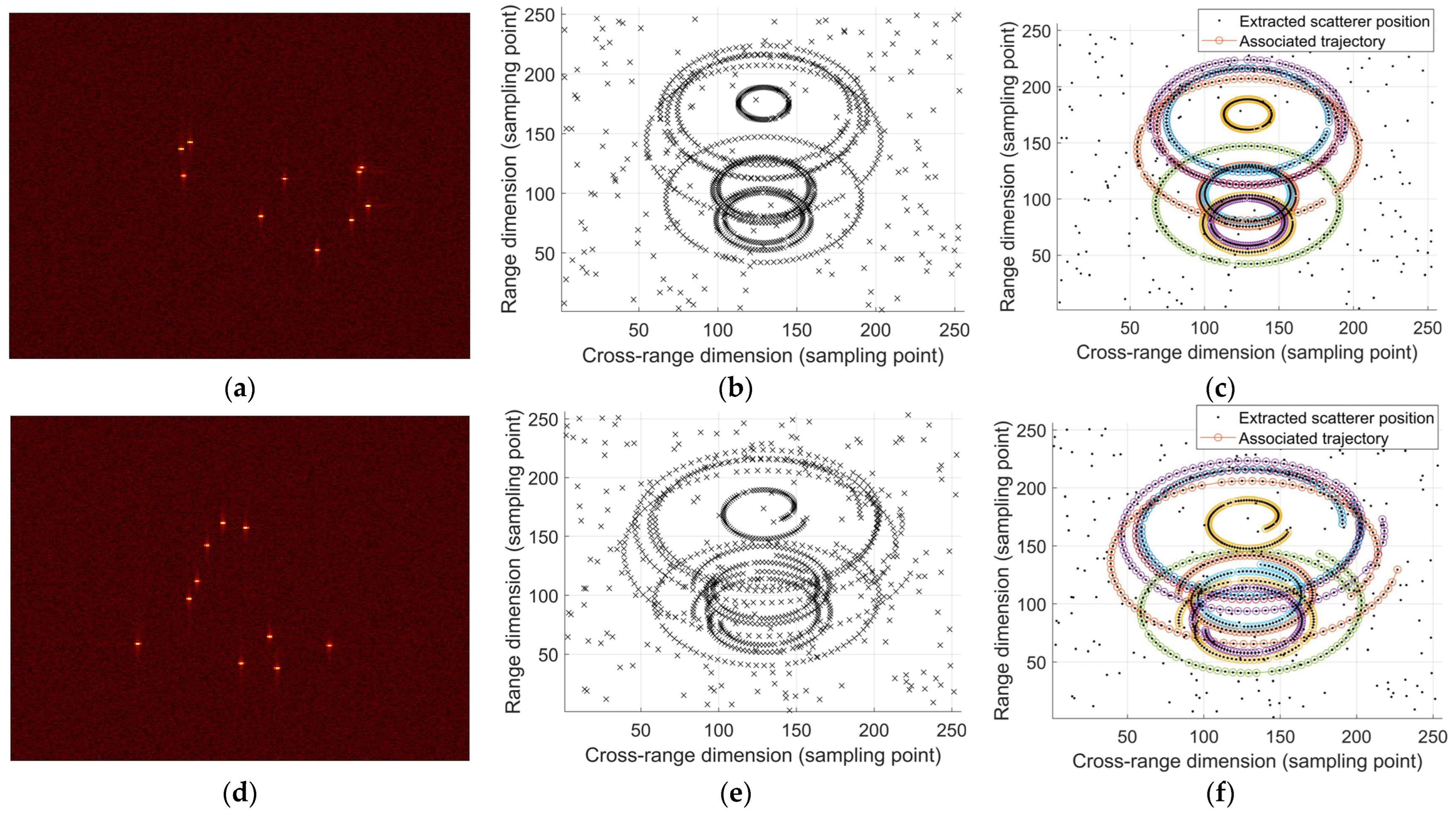
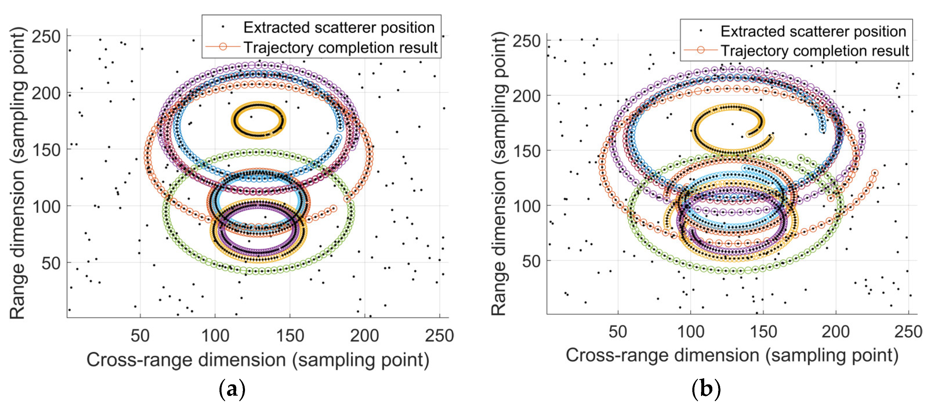
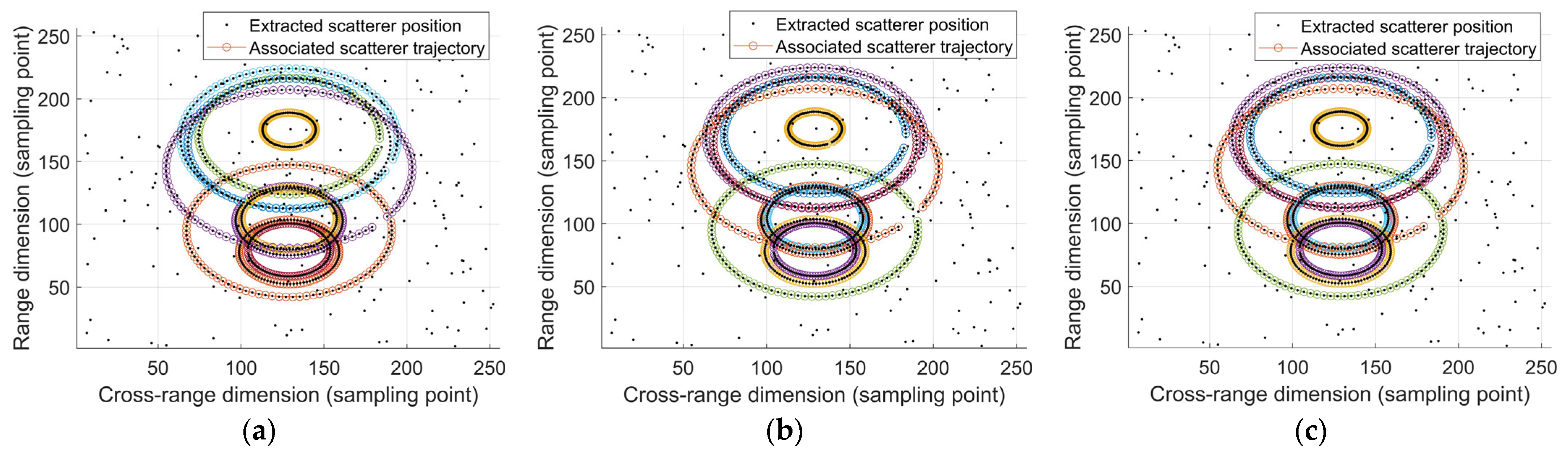
5.1. Effectiveness Analysis

To verify the effectiveness of the proposed algorithm, a simulated point model comprising 10 randomly selected points has been constructed. The details of the point model are shown in Figure 4.

Figure 4. Target model with 10 randomly selected points.

The simulated radar operates in X-band with a signal bandwidth of 1 GHz. Corresponding parameters of the observation scenario are detailed in Table 1. To assess the performance of the proposed algorithm, particularly its handling of non-elliptical trajectories, two distinct scenarios are designed. The first scenario generates elliptical trajectories, where the azimuth angle of the radar LOS changes with the observation time, while the pitch angle remains constant. Concurrently, the attitude of the space target remains unchanged throughout the observation period. In the second scenario, the space target spins around an arbitrary axis, simulating a simultaneous change in both the azimuth and pitch angles of the radar LOS, in addition to the azimuth angle variation. The specific parameters for these scenarios are presented in Table 1.

Table 1. Observation parameters of the scenarios with elliptical trajectories and non-elliptical trajectories.

Parameters	Values
	Elliptical Trajectories	Non-Elliptical Trajectories
Total observation time (second)	92	92
Image frame number	92	92
Range of the variation of the azimuth angle of the radar LOS (degree)	[0, 360] *	[0, 360] *
The pitch angle of the radar LOS (degree)	45	45
Rotation angular velocity (degree/s)	0	0.6
Pitch angle of the spin axis of the space target (degree)	0	10
Azimuth angle of the spin axis of the space target (degree)	0	5

* [a, b] denotes the variable ranging from a to b.

Based on the configured observation scenario, we have acquired a total of 12,000 echoes for each scenario. These echoes are segmented into 92 sub-apertures, with each sub-aperture having a window length of 256 and a step size of 128. Subsequently, the RD imaging algorithm is applied to each scenario, yielding 92 frames of ISAR images. To these imaging results, Gaussian white noise with a signal-to-noise ratio (SNR) of 10 dB is added. Some of the ISAR images are shown in Figure 5a,d. Following this, the 2D-ESPRIT algorithm [11] is utilized to extract the scattering centers from the sequential ISAR images under the two observation scenarios, as shown in Figure 5b,e. It is evident from Figure 5b,e that there are numerous false alarm points and leakage detections. Based on the scattering center extraction results, the detection probability of each scatterer is set to 0.95, and the clutter density is set to 3 × 10⁻⁵ per square pixel. The image size is 256 × 256 pixels.

Figure 5. Imaging results and trajectory association results under two different observation scenarios. (a) First image of the space target with elliptical trajectories. (b) The scatterer extraction results of the space target with elliptical trajectories. (c) Trajectory association results of the space target with elliptical trajectories where each color represents one associated trajectory. (d) 22nd image of the space target with non-elliptical trajectories. (e) The scatterer extraction results of the space target with non-elliptical trajectories. (f) Trajectory association results of the space target with non-elliptical trajectories where each color represents one associated trajectory.

The proposed ML-GM-PHD filtering algorithm is applied to obtain the trajectory association results in the two observation scenarios, as illustrated in Figure 5c,f. The trajectories of different scatterers are represented by curves of distinct colors. It is evident that the proposed method achieves excellent trajectory association performance in both the scenarios. Since the filtering process incorporates a high-maneuvering motion model, the constraint of elliptical motion is no longer a mandatory requirement. Additionally, the proposed method is capable of filtering out clutter and estimating missing detections, thereby demonstrating robustness in complex environments.

To quantitatively assess the performance of the proposed algorithm, we define metrics for accuracy and error rate in trajectory association. Let $N_{total}$, $N_{true}$, and $N_{false}$ denote the number of real scatterers, correctly associated scatterers, and incorrectly associated scatterers, respectively. The accuracy rate of trajectory association is then defined as follows:

$$\eta ={\displaystyle \frac{N_{true}}{N_{total}}}\times 100\%$$

(46)

The error rate of trajectory association is defined as follows:

$$\epsilon ={\displaystyle \frac{N_{false}}{N_{total}}}\times 100\%$$

(47)

In this context, an associated scatterer is deemed correctly associated if its trajectory is complete and its variation aligns with that of a real scatterer. Conversely, if the associated trajectory of a scatterer includes false alarm points or missed detections, that scatterer is considered incorrectly associated.

Therefore, by counting the number of correctly and incorrectly associated scattering centers in two observation scenarios, the accuracy and error rate can be calculated. The evaluation results are detailed in Table 2, which further demonstrates that the proposed algorithm can achieve excellent performance for space targets exhibiting both elliptical and non-elliptical trajectories.

Table 2. Evaluation results of trajectory association performance for the space target with elliptical trajectories and non-elliptical trajectories.

Trajectory Type	Number of Real Scatterers	Number of Correctly Associated Scatterers	Number of Incorrectly Associated Scatterers	Accuracy Rate	Error Rate
Elliptical trajectories	882	882	0	100%	0
Non-elliptical trajectories	879	879	0	100%	0

By applying the proposed method, a complete trajectory matrix can be obtained. Subsequently, a well-scaled trajectory matrix can be obtained by the two-dimensional calibration. The complete trajectories corresponding to the observed targets with elliptical trajectories and non-elliptical trajectories are depicted in Figure 6a and b, respectively. It is evident that the missing trajectory points are estimated with high accuracy. After that, the 3D geometry of the scatterers can be obtained by performing the factorization decomposition on the well-scaled trajectory matrix. The 3D reconstruction results under the two observation scenarios are presented in Figure 6c and d, respectively, demonstrating high reconstruction performance.

Figure 6. Complete scatterer trajectories and 3D reconstruction result. (a) Complete elliptical trajectories of scatterers where each color represents one associated trajectory. (b) Complete non-elliptical trajectories of scatterers where each color represents one associated trajectory. (c) 3D reconstruction result of scatterers with elliptical trajectories. (d) 3D reconstruction result of scatterers with non-elliptical trajectories.

Concurrently, to evaluate the 3D reconstruction performance, the root mean square error (RMSE) metric is defined in this section as follows:

$$E_{RMSE}=\sqrt{{\displaystyle \frac{1}{N}}{\displaystyle \sum _{n=1}^N{\left(p_n^{real}-p_n^{reconstructed}\right)}^2}}$$

(48)

where $N$, $p_n^{real}$, and $p_n^{reconstructed}$ denote the scatterer number, the true 3D coordinates of nth scattering center, and the reconstructed 3D coordinates of nth scattering center, respectively. The RMSE metric quantifies the absolute discrepancy between the reconstructed 3D coordinates and the true 3D coordinates of the scattering centers. The poorer the 3D reconstruction performance, the higher the RMSE will be. Conversely, a smaller RMSE indicates better reconstruction performance.

It can be calculated from Equation (48) that the RMSEs for the 3D reconstruction results under the two observation scenarios are 0.0346 m and 0.0391 m, respectively. These values further demonstrate the effectiveness and accuracy of the proposed algorithm.

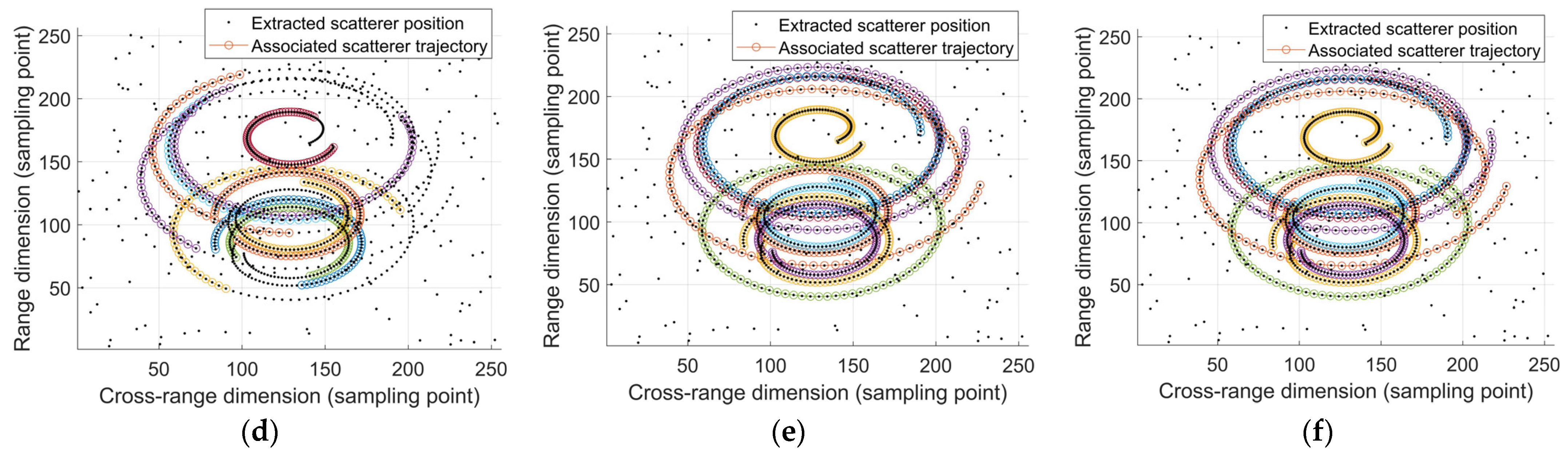
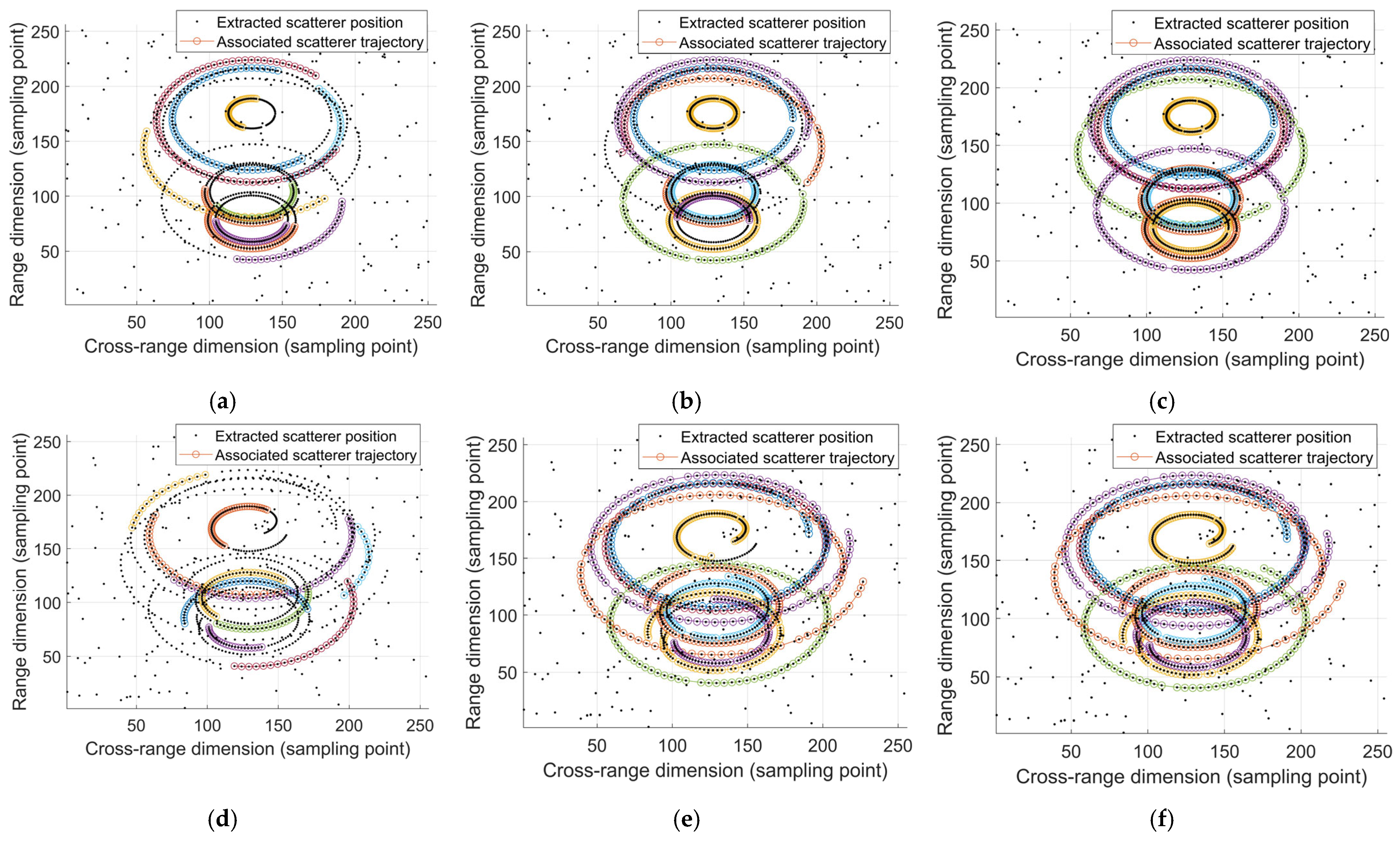
5.2. Performance Comparison and Analysis

To evaluate the performance superiority of the proposed trajectory association algorithm over other classical algorithms, the MCMCDA algorithm [11], the standard L-GM-PHD filtering algorithm [31], and the proposed algorithm are applied in the two observation scenarios as depicted in Figure 4. The trajectory association metrics defined in Equations (46) and (47) are calculated based on the results from these various algorithms. To ascertain the robustness of different algorithms concerning the scatterer detection probability, the comparison experiments are conducted with the detection probability set at 1 and 0.95, respectively.

When the detection probability of the scattering center is set to 1, the trajectory association results of different algorithms are shown in Figure 7. It is evident that the MCMCDA algorithm can achieve satisfactory trajectory association performance, as depicted in Figure 7a, when the scatterer trajectory coincides with an ellipse. However, when the ellipse constraint for the scattering center trajectory is not met, the performance of MCMCDA algorithm declines significantly, as shown in Figure 7d. A substantial number of extracted points fail to be correctly correlated, and there exist cases where multiple points from the same scattering center are incorrectly associated to different trajectories.

Figure 7. Trajectory association results of different algorithms when the scatterer detection probability is set to 1. (a) Trajectory association result of scatterers with elliptical motion model by applying MCMCDA algorithm. (b) Trajectory association result of scatterers with elliptical motion model by applying standard L-GM-PHD algorithm. (c) Trajectory association result of scatterers with elliptical motion model by applying proposed algorithm. (d) Trajectory association result of scatterers with non-elliptical motion model by applying MCMCDA algorithm. (e) Trajectory association result of scatterers with non-elliptical motion model by applying standard L-GM-PHD algorithm. (f) Trajectory association result of scatterers with non-elliptical motion model by applying proposed algorithm.

As for the standard L-GM-PHD algorithm and the proposed algorithm, better trajectory association performance is achieved than the MCMCDA algorithm since the current motion model is used. The trajectory association results are shown in Figure 7b,c,e,f. However, since the weight accumulation of the Gaussian components is needed in the standard L-GM-PHD algorithm to confirm a trajectory, it is difficult to associate the several initial points of each trajectory. The proposed algorithm solves this problem by designing bidirectional trajectory association processing and a trajectory fusion mechanism to obtain complete and accurate trajectories.

The trajectory association evaluation results of different algorithms in the two observation scenarios are detailed in Table 3. It can be noted that the proposed method outperforms both MCMCDA and L-GM-PHD algorithms in terms of trajectory association accuracy, under both the elliptical and non-elliptical trajectory scenarios.

Table 3. Trajectory association performance evaluation results when the scatterer detection probability is set as 1.

Trajectory Type	Elliptical Trajectories			Non-Elliptical Trajectories
Number of real scatterers	920			920
Algorithm	MCMCDA	L-GM-PHD	Proposed algorithm	MCMCDA	L-GM-PHD	Proposed algorithm
Number of correctly associated scatterers	891	909	920	553	907	920
Number of incorrectly associated scatterers	1	0	0	1	0	0
Accuracy rate (%)	96.85	98.8	100	60.11	98.59	100
Error rate (%)	0.11	0	0	0.11	0	0

Similarly, when the scattering center detection probability is set to 0.95, the trajectory association results of different algorithms are shown in Figure 8. As shown in Figure 8a,d, the MCMCDA algorithm exhibits numerous missing points and incorrect associations in the trajectory association results. This is because the MCMCDA algorithm does not account for interruptions and missed detections. As for the L-GM-PHD algorithm, since the PHD of newly detected scatterers is preset, it tends to create fragmented trajectories under missed detection conditions. Therefore, a normal scatterer trajectory may be segmented into two or more distinct trajectories, as illustrated in Figure 8b,e. Additionally, the confirmation of each trajectory in the L-GM-PHD method relies on the cumulative weight of each Gaussian component, which means that the initial points before trajectory confirmation often fail to associate successfully, resulting in a reduced accuracy rate. In contrast, the proposed method demonstrates robustness and achieves superior trajectory association performance, as shown in Figure 8c,f.

Figure 8. Trajectory association results of different algorithms when the scatterer detection probability is set to 0.95. (a) Trajectory association result of scatterers with elliptical motion model by applying MCMCDA algorithm. (b) Trajectory association result of scatterers with elliptical motion model by applying standard L-GM-PHD algorithm. (c) Trajectory association result of scatterers with elliptical motion model by applying proposed algorithm. (d) Trajectory association result of scatterers with non-elliptical motion model by applying MCMCDA algorithm. (e) Trajectory association result of scatterers with non-elliptical motion model by applying standard L-GM-PHD algorithm. (f) Trajectory association result of scatterers with non-elliptical motion model by applying proposed algorithm.

Similarly, comparative results of the trajectory association metrics of each algorithm can be obtained by calculating the accuracy rate and error rate for elliptical and non-elliptical trajectory targets, as shown in Table 4. It is evident that the performance of both the MCMCDA algorithm and the L-GM-PHD algorithm declines significantly in the presence of the missed detection of scattering centers. In contrast, the proposed algorithm demonstrates higher accuracy and stability of trajectory association under such conditions.

Table 4. Trajectory association performance evaluation results when the scatterer detection probability is set as 0.95.

Trajectory Type	Elliptical Trajectories			Non-Elliptical Trajectories
Number of real scatterers	886			868
Method	MCMCDA	L-GM-PHD	Proposed algorithm	MCMCDA	L-GM-PHD	Proposed algorithm
Number of correctly associated scatterers	448	696	886	317	805	868
Number of incorrectly associated scatterers	0	1	0	0	2	1
Accuracy rate (%)	50.56	78.56	100	36.52	92.74	100
Error rate (%)	0	0.11	0	0	0.23	0.12

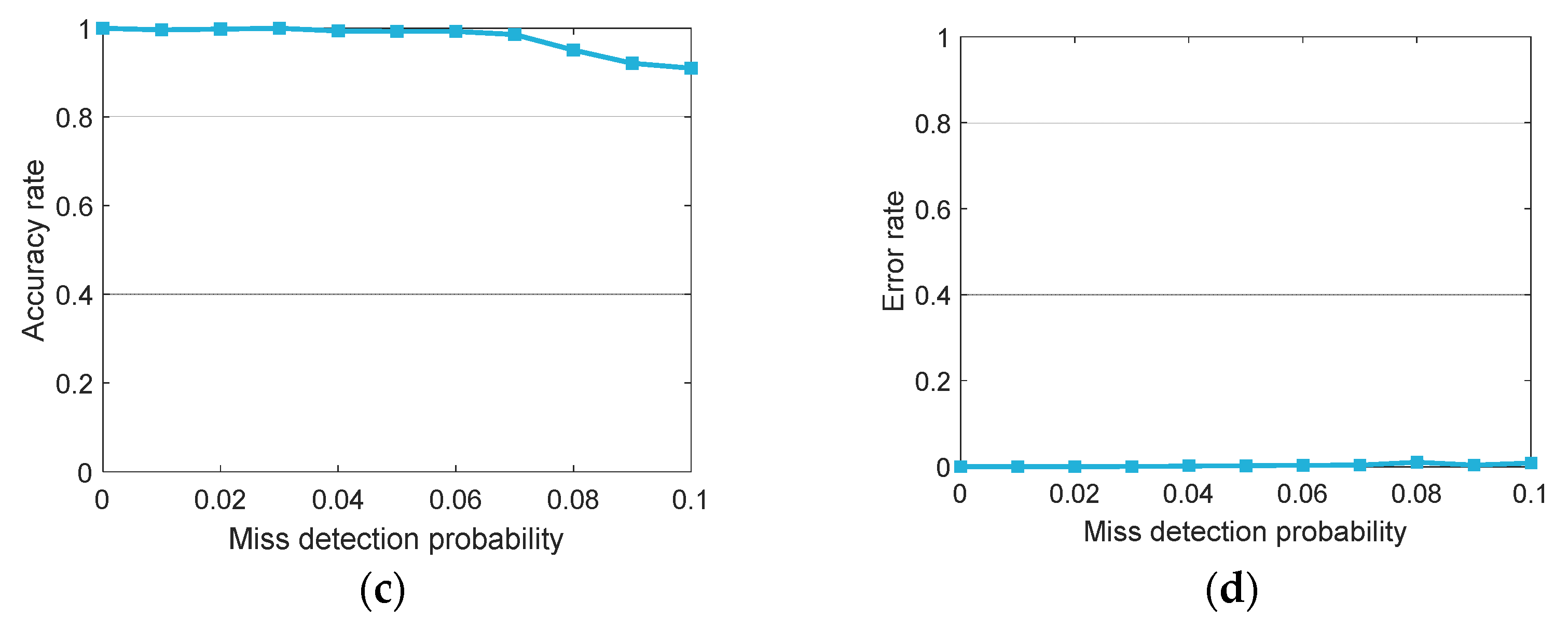
5.3. Algorithm Robustness Analysis

As detailed in Section IV, the algorithm’s performance is dependent on the accuracy of scatterer extraction and the probability of scatterer detection. To further verify the robustness of the proposed algorithm, Monte Carlo simulations are conducted in this section, varying both the scatterer extraction errors and the scatterer detection probabilities. The point target model and the observation scenario used are consistent with those described in the preceding subsection.

To evaluate the performance of the trajectory association algorithm under varying degrees of scattering center extraction error, random bias is introduced into the ideal extraction positions of the scatterers. For the sake of generality, this bias is selected to follow a Gaussian distribution, with the standard deviation ranging from 0 to 0.5 sampling points in increments of 0.05 sampling points. Under each level of bias, 50 Monte Carlo simulation experiments are performed. The trajectory association evaluation metrics are computed and statistically analyzed, as depicted in Figure 9a,b. The experimental results demonstrate the robustness of the proposed method against the scattering center extraction errors. The accuracy rate of trajectory association exceeds 90%, and the error rate remains below 1% when the standard deviation of the position bias is less than 0.3 sampling points.

Figure 9. Performance variation curves of the proposed algorithm under different scatterer extraction errors and detection probabilities. (a) Scatterer association accuracy rate variation curve with the scatterer extraction error. (b) Scatterer association error rate variation curve with the scatterer extraction error. (c) Scatterer association accuracy rate variation curve with the scatterer detection probability. (d) Scatterer association error rate variation curve with the scatterer detection probability.

Concurrently, to analyze the performance sensitivity of the proposed algorithm to the different scattering center detection probabilities, the detection probability is varied linearly from 0.9 to 1, with a step size of 0.01. For each detection probability setting, 50 Monte Carlo experiments are conducted. The accuracy and error rates of the trajectory association results are calculated and analyzed, as presented in Figure 9c,d. The experimental results reveal that the proposed algorithm demonstrates robustness across a range of scatterer detection probabilities. High accuracy rates and low error rates in trajectory association are attainable when the scatterer detection probability exceeds 0.9.

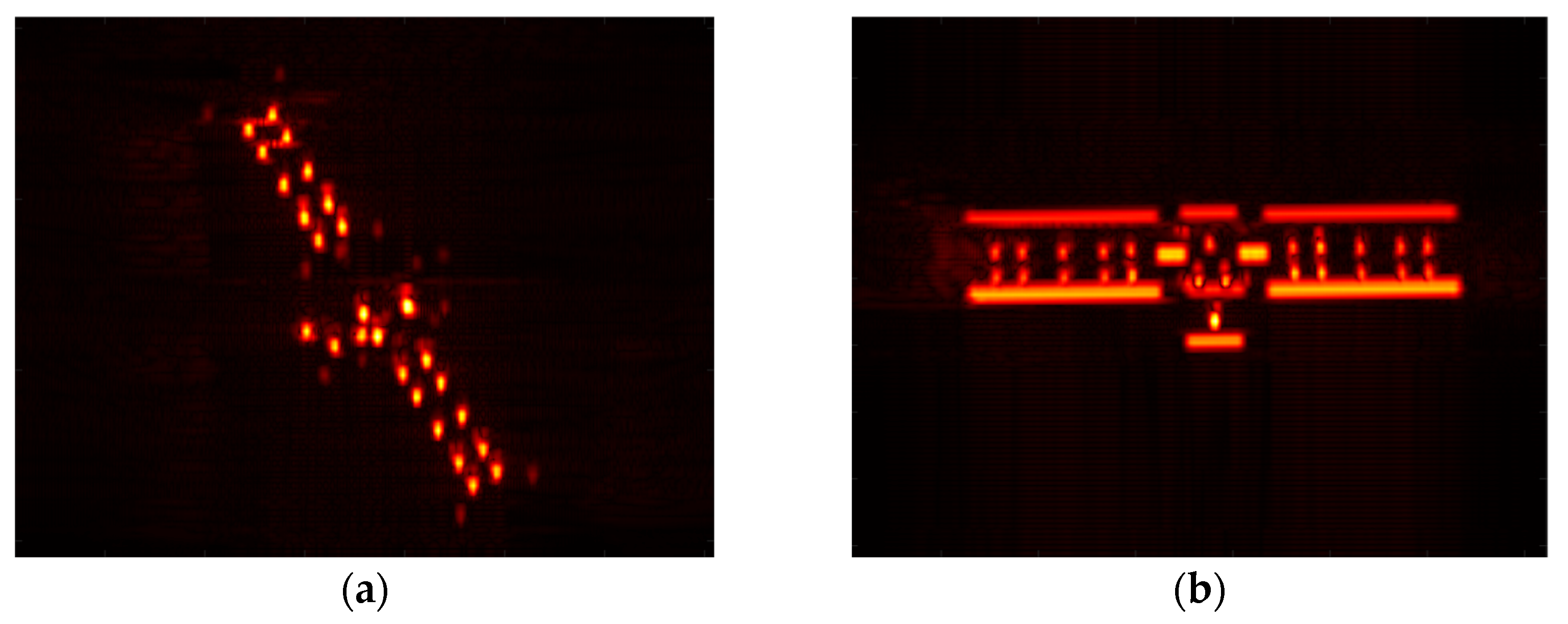
5.4. Experimental Results on Electromagnetical Data

To verify the effectiveness of the proposed method on electromagnetic data, a CAD model of a space target, as depicted in Figure 10e is constructed in this subsection. The simulated radar works in the X-band with a bandwidth of 2 GHz. The radar observation parameters and target motion parameters are detailed in Table 1, with the azimuth angle of the radar LOS ranging from 0 to 100°. A total of 4096 echoes are acquired through electromagnetic computing, which are then divided into 31 sub-apertures. The RD imaging algorithm is applied to each sub-aperture, yielding 31 image frames, with the 13th and 24th frames displayed in Figure 10a and Figure 10b, respectively. The position matrix for each major scattering center is manually extracted from the ISAR image sequence, as shown in Figure 10c. Subsequently, the scatterer trajectories are associated using the proposed method, with the association results presented in Figure 10d. It is evident that accurate and complete trajectories for each scatterer are obtained. Utilizing the trajectory matrix, the 3D positions of the dominant scatterers of the target, as shown in Figure 10f, can be obtained by applying the factorization decomposition. Compared with Figure 10e, it is clear that the precise 3D positions of the dominant scatterers are achieved, with a maximum reconstruction position error of 0.03m.

Figure 10. Experimental results on electromagnetic data. (a) Sixth image. (b) 17th image. (c) Scatterer extraction results. (d) Trajectory association results. (e) CAD model of a satellite. (f) 3D reconstruction result.

6. Conclusions

Aiming at the trajectory association challenge of scattering centers in sequential ISAR images, a modified label mixture Gaussian probability hypothesis density filtering algorithm is proposed. The proposed algorithm overcomes dependence on the elliptical motion constraint of the traditional algorithms and can effectively deal with the interruption and missing detection phenomenon. Moreover, the effectiveness and performance superiority of the proposed method have been verified by utilizing the point target data with randomly distributed positions and electromagnetic data of a space target. However, there still exist several challenges when applied in real data, e.g., precise scatterer extraction of practical ISAR image, image blurring induced by the unknown target motion, etc. In the future, scatterer extraction and focused imaging processing of the real data of space targets will be studied, which can serve as the basis for the effectiveness verification of the proposed method in real data.

References

- Gong, R.; Wang, L.; Wu, B.; Zhang, G.; Zhu, D. Optimal Space-Borne ISAR Imaging of Space Objects with Co-Maximization of Doppler Spread and Spacecraft Component Area. Remote Sens. 2024, 16, 1037. [Google Scholar] [CrossRef]
- Zhao, L.; Wang, J.; Su, J.; Luo, H. Spatial Feature-Based ISAR Image Registration for Space Targets. Remote Sens. 2024, 16, 3625. [Google Scholar] [CrossRef]
- Li, W.; Yuan, Y.; Zhang, Y.; Luo, Y. Unblurring ISAR Imaging for Maneuvering Target Based on UFGAN. Remote Sens. 2022, 14, 5270. [Google Scholar] [CrossRef]
- Anger, S.; Jirousek, M.; Dill, S.; Peichl, M. Inverse Synthetic Aperture Radar Imaging of Space Targets Using Wideband Pseudo-Noise Signals with Low Peak-to-Average Power Ratio. Remote Sens. 2024, 16, 1809. [Google Scholar] [CrossRef]
- Yang, S.; Jiang, W.; Tian, B. ISAR Image matching and 3D reconstruction based on improved SIFT Method. In Proceedings of the 2019 International Conference on Electronic Engineering and Informatics, Nanjing, China, 8–10 November 2019; pp. 224–228. [Google Scholar] [CrossRef]
- Xu, D.; Bie, B.; Sun, G.-C.; Xing, M.; Pascazio, V. ISAR Image Matching and Three-Dimensional Scattering Imaging Based on Extracted Dominant Scatterers. Remote Sens. 2020, 12, 2699. [Google Scholar] [CrossRef]
- Di, G.; Su, F.; Yang, H.; Fu, S. ISAR Image Scattering Center Association Based on Speeded-up Robust Features. Multimed. Tools Appl. 2020, 79, 5065–5082. [Google Scholar] [CrossRef]
- Wang, X.; Guo, B.F.; Shang, C.X. 3D Reconstruction of Target Geometry Based on 2D Data of Inverse Synthetic Aperture Radar Images. J. Electron. Informa. Tech. 2013, 35, 2475–2480. [Google Scholar] [CrossRef]
- Wang, F.; Xu, F.; Jin, Y.Q. Three-Dimensional Reconstruction from a Multiview Sequence of Sparse ISAR Imaging of a Space Target. IEEE Trans. Geosci. Remote Sens. 2018, 56, 611–620. [Google Scholar] [CrossRef]
- Du, R.; Liu, L.; Bai, X.; Zhou, F. A New Scatterer Trajectory Association Method for ISAR Image Sequence Utilizing Multiple Hypothesis Tracking Algorithm. IEEE Trans. Geosci. Remote Sens. 2022, 60, 5103213. [Google Scholar] [CrossRef]
- Liu, L.; Zhou, F.; Bai, X.R. Method for Scatterer Trajectory Association of Sequential ISAR Images Based on Markov Chain Monte Carlo Algorithm. IET Radar Sonar Navig. 2018, 12, 1535–1542. [Google Scholar] [CrossRef]
- Bi, Y.; Wei, S.; Wang, J.; Zhang, Y.; Sun, Z.; Yuan, C. New Method of Scatterers Association and 3D Reconstruction Based on Multi-Hypothesis Tracking. J. Beijing Uni. Aeronaut. Astronaut. 2016, 42, 1219–1227. [Google Scholar] [CrossRef]
- Liu, L.; Zhou, F.; Bai, X.R.; Paisley, J.; Ji, H. A Modified EM Algorithm for ISAR Scatterer Trajectory Matrix Completion. IEEE Trans. Geosci. Remote Sens. 2018, 56, 3953–3962. [Google Scholar] [CrossRef]
- Liu, L.; Zhou, F.; Bai, X.R.; Tao, M.L.; Zhang, Z.J. Joint Cross-Range Scaling and 3D Geometry Reconstruction of ISAR Targets Based on Factorization Method. IEEE Trans. Image Process. 2016, 25, 1740–1750. [Google Scholar] [CrossRef]
- Shang, S.; Li, M.; Hou, Y.; Yu, J. 3D Target reconstruction based on the ISAR image sequence. In Proceedings of the 12th European Conference on Synthetic Aperture Radar, Aachen, Germany, 4–7 June 2018; pp. 1142–1146. [Google Scholar]
- Xu, D.; Xing, M.; Xia, X.-G.; Sun, G.-C.; Fu, J.; Su, T. A Multi-Perspective 3D Reconstruction Method with Single Perspective Instantaneous Target Attitude Estimation. Remote Sens. 2019, 11, 1277. [Google Scholar] [CrossRef]
- Zhou, C.; Jiang, L.; Yang, Q.; Ren, X.; Wang, Z. High Precision Cross-Range Scaling and 3D Geometry Reconstruction of ISAR Targets Based on Geometrical Analysis. IEEE Access 2020, 8, 132415–132423. [Google Scholar] [CrossRef]
- Li, G.; Liu, Y.; Wu, L.; Xu, S.; Chen, Z. Three-Dimensional Reconstruction Using ISAR Sequences. In Proceedings of the 8th International Symposium on Multispectral Image Processing and Pattern Recognition, Wuhan, China, 26–27 October 2013; p. 8919. [Google Scholar] [CrossRef]
- Zhou, Y.; Zhang, L.; Xing, C.; Xie, P.; Cao, Y. Target Three-Dimensional Reconstruction from the Multi-view Radar Image Sequence. IEEE Access 2019, 7, 36722–36735. [Google Scholar] [CrossRef]
- Liu, L.; Zhou, Z.B.; Zhou, F.; Shi, X. A New 3-D Geometry Reconstruction Method of Space Target Utilizing the Scatterer Energy Accumulation of ISAR Image Sequence. IEEE Trans. Geosci. Remote Sens. 2020, 58, 8345–8357. [Google Scholar] [CrossRef]
- Zhou, Z.; Liu, L.; Du, R.; Zhou, F. Three-Dimensional Geometry Reconstruction Method for Slowly Rotating Space Targets utilizing ISAR Image Sequence. Remote Sens. 2022, 14, 1114. [Google Scholar] [CrossRef]
- Zhou, Z.; Jin, X.; Liu, L.; Zhou, F. Three-Dimensional Geometry Reconstruction Method from Multi-View ISAR Images Utilizing Deep Learning. Remote Sens. 2023, 15, 1882. [Google Scholar] [CrossRef]
- Mahler, R.P.S. Multitarget Bayes Filtering via First-order Multitarget Moments. IEEE Trans. Aerosp. Electron. Syst. 2003, 39, 1152–1178. [Google Scholar] [CrossRef]
- Vo, B.N.; Vo, B.T.; Phung, D. Labeled Random Finite Sets and the Bayes Multi-Target Tracking Filter. IEEE Trans. Signal Process. 2014, 62, 6554–6567. [Google Scholar] [CrossRef]
- Hesar, H.D.; Abrishami Moghaddam, H.; Safari, A.; Eftekhari-Yazdi, P. Multiple Sperm Tracking in Microscopic Videos Using Modified GM-PHD filter. Mach. Vis. Appl. 2018, 29, 433–451. [Google Scholar] [CrossRef]
- Vo, B.N.; Ma, W.K. The Gaussian Mixture Probability Hypothesis Density Filter. IEEE Trans. Signal Process. 2006, 54, 4091–4104. [Google Scholar] [CrossRef]
- Mahler, R. PHD Filters of Higher Order in Target Number. IEEE Trans. Aerosp. Electron. Syst. 2007, 43, 1523–1543. [Google Scholar] [CrossRef]
- Vo, B.N.; Singh, S.; Doucet, A. Random Finite Sets and Sequential Monte Carlo Methods in Multi-Target Tracking. In Proceedings of the International Conference on Radar, Adelaide, SA, Australia, 3–5 September 2003; pp. 486–491. [Google Scholar] [CrossRef]
- Vo, B.N.; Singh, S.; Doucet, A. Sequential Monte Carlo Implementation of the PHD Filter for Multi-Target Tracking. In Proceedings of the 6th International Conference of Information Fusion, Cairns, QLD, Australia, 8–11 July 2003; pp. 792–799. [Google Scholar] [CrossRef]
- Panta, K.; Clark, D.E.; Vo, B.N. Data Association and Track Management for the Gaussian Mixture Probability Hypothesis Density Filter. IEEE Trans. Aerosp. Electron. Syst. 2009, 45, 1003–1016. [Google Scholar] [CrossRef]
- Clark, D.E.; Panta, K.; Vo, B.N. The GM-PHD Filter Multiple Target Tracker. In Proceedings of the 9th International Conference on Information Fusion, Florence, Italy, 10–13 July 2006. [Google Scholar] [CrossRef]
- Zhou, H. A "Current" Statistical Model and Adaptive Tracking Algorithm for Maneuvering Targets. Acta Aeronaut. Astronaut. Sin. 1983, 4, 73–86. [Google Scholar] [CrossRef]
- Zhang, S.; Liu, Y.; Li, X.; Bi, G. Fast ISAR Cross-Range Scaling Using Modified Newton Method. IEEE Trans. Aerosp. Electron. Syst. 2018, 54, 1355–1367. [Google Scholar] [CrossRef]
- Wang, Y.; Huang, X.; Zhang, Q. Rotation Parameters Estimation and Cross-Range Scaling Research for Range Instantaneous Doppler ISAR Images. IEEE Sens. J. 2020, 20, 7010–7020. [Google Scholar] [CrossRef]
Disclaimer/Publisher’s Note: The statements, opinions and data contained in all publications are solely those of the individual author(s) and contributor(s) and not of MDPI and/or the editor(s). MDPI and/or the editor(s) disclaim responsibility for any injury to people or property resulting from any ideas, methods, instructions or products referred to in the content. |
© 2025 by the authors. Licensee MDPI, Basel, Switzerland. This article is an open access article distributed under the terms and conditions of the Creative Commons Attribution (CC BY) license (https://creativecommons.org/licenses/by/4.0/).