Reconstruction of Effective Cross-Sections from DEMs and Water Surface Elevation

Abstract

Knowledge of river bathymetry is crucial for accurately simulating river flows and floodplain inundation. However, field data are scarce, and the depth and shape of the river channels cannot be systematically observed via remote sensing. Therefore, an efficient methodology is necessary to define effective river bathymetry. This research reconstructs the bathymetry from existing global digital elevation models (DEMs) and water surface elevation observations with minimum human intervention. The methodology can be considered a 1D geometric inverse problem, and it can potentially be used in gauged or ungauged basins worldwide. Nine global DEMs and two sources of water surface elevation (in situ and remotely sensed) were analyzed across two study areas. Results highlighted the importance of preprocessing cross-sections to align with water surface elevations, significantly improving discharge estimates. Among the techniques tested, one that combines the slope-break concept with the principles of mass conservation consistently provided robust discharge estimates for the different DEMs, achieving good performance in both study areas. Copernicus and FABDEM emerged as the most reliable DEMs for accurately representing river geometry. Overall, the proposed methodology offers a scalable and efficient solution for cross-section reconstruction, supporting global hydraulic modeling in data-scarce regions.

1. Introduction

Monitoring river discharge is crucial for managing water resources, predicting floods, and understanding the global water cycle. Traditional approaches to monitoring rely heavily on in situ stations, which are sparsely distributed around the globe. The advent of satellite remote sensing (RS) has introduced novel approaches to discharge estimation [1]. However, the inability to directly measure river bathymetry using satellite instruments limits the accuracy of RS-based river flow estimates.

Global digital elevation models (DEMs) have become essential tools for flood monitoring and hydrological modeling, but improvements are needed for global modeling [2]. Due to limitations in capturing underwater topography, DEMs’ accuracy and resolution often fall short over water surfaces. This underlines the necessity of incorporating underwater bathymetric data. Neglecting bathymetry leads to inaccuracies in discharge estimation and flood forecasting, particularly at high-frequency small flood events [3].

The reconstruction of river bathymetry has traditionally relied on in situ surveys, such as Acoustic Doppler Current Profilers (ADCPs). While precise, these methods are costly, time-consuming, and impractical for large-scale or global applications. Recent advancements have focused on techniques applied to remotely sensed (RS) data. Some build the bathymetry entirely from RS observations of width and elevation [4,5,6]. In contrast, others modify the elevations of rivers in digital elevation models through geometrical or hydraulic considerations [3,7].

These methods can be broadly classified into six categories, with increasing degrees of complexity:

• Slope-break (SB) methods, which identify inflection points in the cross-section profiles to accommodate different flow conditions [6,7,8,9,10];
• Channel Bankfull (CB) methods, which seek to find the relationship between channel width, depth, and bankfull discharge using power laws [11,12,13,14];
• Hypsometric curves, which relate surface area and elevation to infer depth [5,15];
• Discharge inversion methods, which build the bathymetry from mass conservation principles [3,16,17];
• Data assimilation techniques, which reconstruct the bathymetry by integrating observational and model data [4,18,19,20,21];
• Artificial intelligence approaches have been employed for bathymetry estimation [22,23].

Despite their advancements, the existing methodologies face several limitations that this study aims to address. Although advanced data assimilation techniques and artificial intelligence show potential, their higher computational demands make them unsuitable for a global simplified approach. In a comparison between the SB method and the CB method [7], it was found that the former outperforms the latter in capturing channel depth and flow dynamics in data-sparse regions, making the slope-break method more suitable for this study. However, previous applications of the SB method were restricted to a single DEM. They did not incorporate more recent and accurate products, such as the Copernicus DEM [24], which has demonstrated superior hydraulic modeling performance [25,26]. Additionally, the slope-break methodology often neglects the continuity of the cross-section shape along the river, which might lead to abrupt changes in hydraulic estimates that compromise their reliability. Incorporating mass-conservation principles could mitigate these limitations by ensuring more consistent cross-sectional profiles.

Furthermore, some studies treat bathymetry as the sole source of uncertainty, overlooking the errors in water surface elevation observations, which may be very significant when using remotely sensed measurements [14,27]. This study addresses these gaps by exploring the impact of DEM choice, preprocessing techniques, and water surface elevation data sources on discharge estimation and bathymetry reconstruction.

In the context of global discharge estimation, the main objective of the research is to reconstruct full bathymetry as cross-sections at predefined nodes. This study is organized into seven sections. Section 2 explains the methods to extract the bathymetry from DEMs, to preprocess them, and to estimate the discharge. Section 3 details the remotely sensed datasets used: the nine global digital elevation models and the water surface elevation data. Section 4 characterizes the study areas selected due to the availability of comprehensive bathymetric reference data. Section 5 contains the results, which are further analyzed in the discussion (Section 6). The last section gives general conclusions and further recommendations.

2. Methods

In the methodology, the following notations are used:

• $t$—time; $x$—coordinate along the river centerline, $z$—vertical coordinate;
• $\left\{t_i\right\}, i=1, \dots , N_t$—set of time instants;
• $\left\{x_j\right\},j=1, \dots , N_x$—set of spatial nodes;
• $h\left(x_j,t_i\right)$—the water surface elevation, counted along the $z$-axis, at node $x_j$ and time instant $t_i$;
• $w\left(x_j, z\right)$—the cross-section width as a function of $z$ at node $x_j$;
• $Q\left(x_j,t_i\right)$—the discharge at node $x_j$ and time instant $t_i$;
• $h_{min}\left(x_j\right)$—the lowest water surface elevation observed at node $x_j, \forall t$;
• $h_{max}\left(x_j\right)$—the highest water surface elevation observed at node $x_j, \forall t$;
• $z_b\left(x_j\right)$—the cross-section bottom elevation at node $x_j$;
• $w_b\left(x_j\right)$—the cross-section bottom width at node $x_j$, $z=z_b\left(x_j\right)$;
• $b\left(x_j\right)=w\left(x_j,z_b\left(x_j\right)\right)$—the base of a rectangular cross-section;
• $z_{max}\left(x_j\right)$—the cross-section top elevation at node $x_j$;
• $w_{max}\left(x_j\right)$—the cross-section top width at node $x_j$, $z=z_{max}\left(x_j\right)$.

The methodological steps are illustrated in the flowchart in Figure 1. The methodology is designed for a single or connected set of reaches without tributaries. The required inputs are a water mask, the location of the nodes, a DEM, water surface elevation observations, and a prior mean discharge. The outputs are 1D cross-sections located at pre-defined nodes, discharge, and roughness estimates. The general steps of the methodology are explained here, while more details for specific inputs or processes are given in subsections, which are mentioned in the flowchart.

The methods can be divided into two main parts: dry and wet bathymetry estimation. In this study, we define dry bathymetry as a part of the cross-section (cs) where we have some observed data. These can be the bed elevation from the DEMs and/or the water surface elevation ($h$) obtained in situ or remotely sensed. The wet bathymetry of the river channel is where no information regarding widths or elevations is available.

Figure 2 illustrates cross-section profiles at a node and clarifies the idea of bathymetry division. The different profiles in this figure correspond to one of the blue boxes in Figure 1. The solid brown line is the symmetrical cs built from a DEM. It can be considered a first reconstruction of the dry bathymetry, and it depends only on the input DEM. At the end of this step, the bottom elevation of the cs $\left({z_b}_0\right)$ does not necessarily coincide with the lowest observed water surface elevation $\left(h_{min}\right)$, the lowest inverted blue triangle in Figure 2. We then preprocess the symmetrical cs using $h$ provided by in situ or virtual stations. In this process, we have information on $h$ but only partial knowledge of the width ($w$); the relationship between width and height is unknown when $z$ is smaller than ${z_b}_0$, $w\left(x_j, z\right)=?, \mathrm{z}\in \left[h_{min}\left(x_j\right),{z_b}_0\left(x_j\right)\right]$. Possible preprocessed profiles with varying bottom widths $\left({w_b}_{opt}\right)$ are displayed in dashed green lines in Figure 2. These constitute a second reconstruction of the dry bathymetry. At the end of this step, ${z_b}_1=h_{min}$. Under $h_{min}$ lies the wet bathymetry. In that region, no information on $h$ and $w$ is available, so the bathymetry needs to be estimated using the prior mean discharge $\left({\overline{Q}}_0\right)$ and the associated probability density function. A rectangular shape is assumed; the base is the bottom width of the dry bathymetry, while the unknown depth goes from $h_{min}$ to ${z_b}_2$. Possible outputs of the complete profile (dry and wet bathymetry) are shown in blue dotted lines.

The first step of the methodology is to define the cross-section basic segments $\left(cs\overline{AB}\right)$ to extract the elevation from the DEMs. Passing through defined nodes, these segments link the left riverbank to the right one and are perpendicular to the river centerline. In this study, we use the existing centerlines and nodes from the Surface Water and Ocean Topography (SWOT) River Database (SWORD) [28]. SWORD is a global vector database of river reaches (∼10 km long) and nodes (∼200 m spacing) whose mean width is wider than 30 m. The riverbanks are extracted from the Global Surface Water Occurrence (GSWO) [29], a raster database (∼30 m resolution) that shows where surface water occurred between 1984 and 2021. The delimited basic segments are then used to obtain the elevation from selected global DEMs. The resulting profiles are converted to symmetrical profiles (brown solid line in Figure 2). The definition of the basic segments and the extraction are explained in Section 2.1, while the digital elevation models are further described in Section 3.1.

This study suggests three methods to preprocess the cross-sections and incorporate the water surface elevation information. We call them “cross-section burning”. The idea is inspired by DEM stream burning, in which the DEM pixels’ elevations are modified to better represent flow patterns using auxiliary water masks [30,31]. In DEM stream burning, the pixels are lowered or lifted, creating rectangular shapes. Our cross-section burning procedures define the bottom widths $\left(w_b\left(x_j\right)\right)$, from which we create rectangular channels down to $h_{min}$ (green dashed lines in Figure 2). The preprocessing methods are further detailed in Section 2.2.

To estimate the wet bathymetry, we apply a redesigned version of the Integrated Modified Gauckler–Manning–Strickler (GMS) model, presented in [32]. It allows the discharge, the added depth, and the roughness coefficient to be simultaneously estimated, using a prior mean discharge $\left({\overline{Q}}_0\right)$, defined per study area over the entire study period. This value is extracted from the validation data in this study, allowing a more effective showcase of the impact of the geometry, which is the primary focus of this study.

The integrated GMS method [32] was developed using synthetic test cases that simulated SWOT data. This satellite can provide synchronized information on rivers’ width and elevation. It potentially allows a reconstruction of the river bathymetry up to the lowest observed water surface elevation $\left(h_{min}\right)$. For the bathymetry built from SWOT, the condition $z_b=h_{min}$ is always satisfied, opposing our study, in which the condition is only obtained after preprocessing.

To estimate the wet bathymetry, the authors [32] use a rectangular shape approximation. The rectangle’s base corresponds to the bottom width of the dry bathymetry (${w_b}_{opt}$ in Figure 2), while the added depth is counted from $h_{min}$ down to a certain elevation to be estimated (${z_b}_2$ in Figure 2). To account for various sources of dry bathymetry and water surface elevation data, the approach has been generalized in this study. More details are presented in Section 2.3.

The water surface elevation required for the cs burning and the wet bathymetry estimation can come from ground stations or remote sensors. In this study, we used the observations from in situ stations and traditional altimetry sensors. RS observations are meant to test the methodology’s potential in ungauged basins. We applied the same methods to both sources and did not attempt to combine them. The $h$ obtained from traditional altimetry sensors is located in virtual stations, the intersection points between the satellite’s paths and the rivers. More details on the $h$ from altimetry sensors are presented in Section 3.2.

Water surface elevation data at the node level is needed to reconstruct the bathymetry at this spatial interval. However, both data sources analyzed in this study only provide data at the location of the stations. On the observation date, the time-averaged $h$ s of the nodes between the monitored stations are filled using linear interpolation, considering the available stations and the distance along the river centerline. The long revisit time and the poor spatial sampling of traditional altimetry sensors limit the number of occasions one can apply this linear interpolation approach. When the slope between the virtual stations cannot be computed due to the lack of simultaneous overpasses, we use the average static slope for the set of reaches from IRIS, a database built from ICESat2 measurements [33].

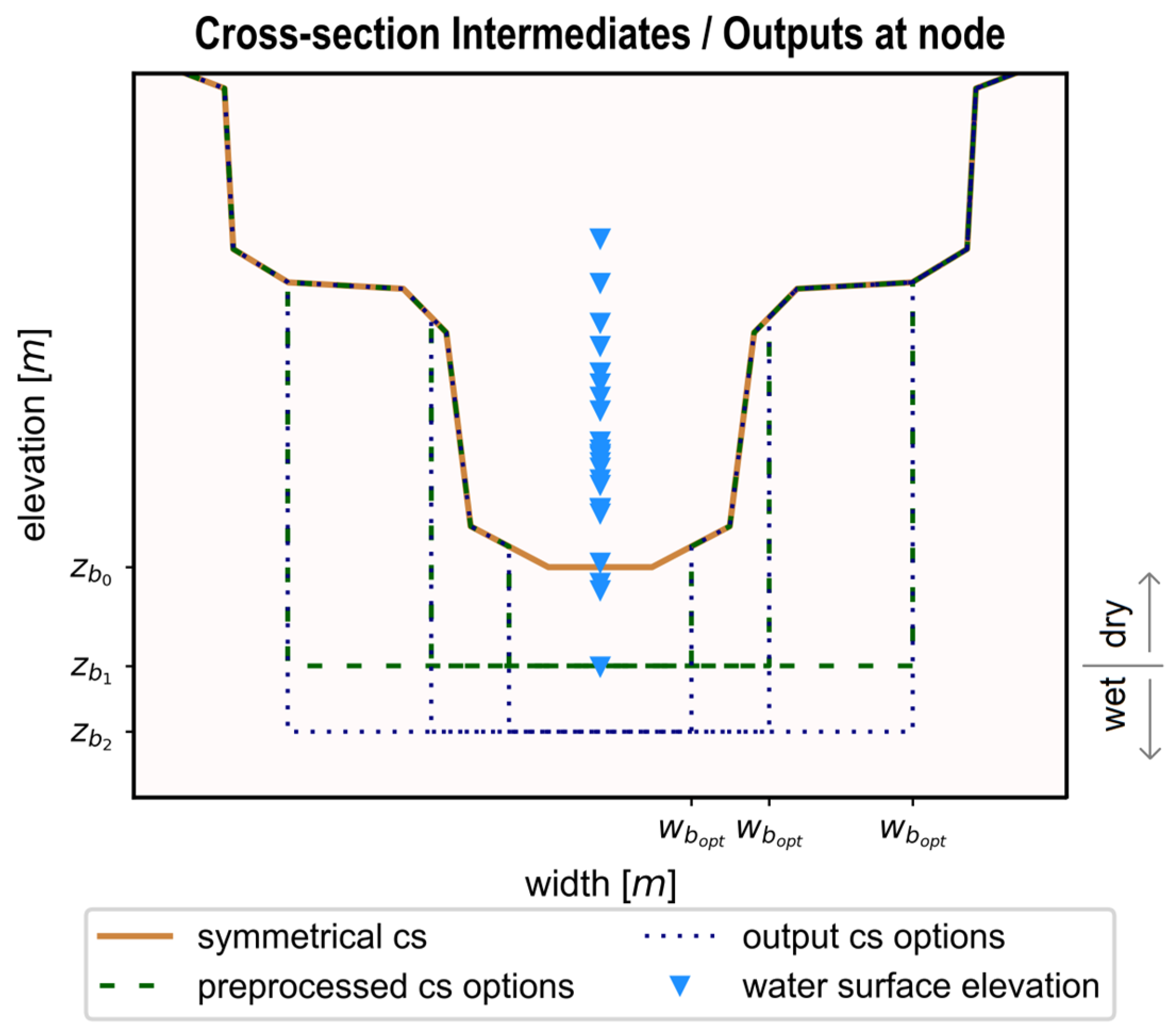
2.1. Cross-Section Definition and Extraction

The cross-section basic segments $\left(cs\overline{AB}\right)$ are defined from point $A\left(x_j,{lon}_a,{lat}_a\right)$ to point $B\left(x_j,{lon}_b,{lat}_b\right)$, in which $lon$ and $lat$ are the projected longitudes and latitudes of the riverbanks for node $x_j$. Three elements are needed to define the segments: location, orientation, and extent. Here, their location is linked to the SWORD nodes, which are distributed along SWORD river centerlines with an approximate 200 m step. To determine the orientation of $cs\overline{AB}\left(x_j\right)$, two points along the river centerline, each one located 100 m away from the node $x_j$, are used to create a perpendicular line.

For the extent of the segments, we use the GSWO masks. An occurrence of 1% is selected to build a binary water mask. This value was chosen to capture high flows but to avoid capturing exceptional flood events. After the binarization, a round of morphological binary closing is performed to bridge small gaps and smooth the boundaries of the water bodies. The centerline is used to define the pixels that belong to the river under study and to exclude adjacent water bodies. The river’s mask is vectorized. The intersection of the perpendicular lines with the vector mask defines the riverbanks for each node, the points $A$ and $B$. The resulting segments match the SWORD nodes and the preprocessed water mask. However, this procedure may result in abrupt changes in angles and the intersection of some segments. When necessary, a manual post-processing step was performed to fix these issues. For a full global approach, these editions can be automated considering the changes in orientation and the presence of intersections.

The cross-section basic segments are used to extract the bed elevation data from the selected DEMs. First, the DEMs are preprocessed so the data refer to the same geoid model (EGM2008) and are projected to the adequate UTM zone. Second, points along $cs\overline{AB}$ are determined with a horizontal one-meter step from the left bank to the right bank. Third, we extract the elevation of each point in each raster DEM. This extraction is performed using a 3 × 3 pixel window, centered in the point. The elevation is a weighted mean of the values of the nine pixels; their weight corresponds to the distance between the pixel center and the desired point. Finally, to delineate the actual riverbanks, we compute the slope from the centerline. As implemented in the Simulation and Integration of Control for Canals software version 5.39a (SIC²) [34], the banks are defined according to the last increasing slope, and points out of these banks are discarded.

The cross-sections are further converted to symmetrical profiles. This is performed by drawing horizontal lines for each elevation, considering a 0.01 m step. We define the parts that are inside of the channel and conserve the width for each elevation. This simplification has been accepted in other studies facing incomplete topographic information and uncalibrated discharge estimates [6,7,9]. The profiles are then simplified using a modified Ramer–Douglas algorithm [35]. It recursively defines which points to keep based on distances from straight lines connecting significant points, preserving the curve’s general shape. This algorithm is further explained in the next section, under the breakpoint method.

Finally, consistency tests have been implemented to verify the profiles; nodes that did not meet these conditions were discarded. The difference between the top and bottom heights must be greater than 0.5 m. The top width must be greater than the one retrieved from the Global River Widths from Landsat (GRWL) [36].

The outputs are simplified symmetrical profiles whose width and elevation were extracted from the DEMs (first blue box in Figure 1 and brown solid lines in Figure 2).

2.2. Cross-Section Burning

As illustrated in Figure 2, we have limited knowledge of the width under the cross-section bottom elevation $\left(z_{b_0}\right)$. At this step, we preprocess the cs to include the information from observed water surface elevations. The methodologies proposed in this study define bottom widths $\left(w_b\right)$ from the symmetrical cross-section profiles. The $w_b$ is then used to create a rectangular channel down to the lowest observed $h$ $\left(h_{min}\right)$. The outputs correspond to the second blue box in Figure 1 and the green dashed lines in Figure 2.

We use three methods to define the bottom width: the “breakpoint” one, based on the slope-break method [7,9]; the “continuity” method, based on the Mass Conservation Flow Inversion (McFLI) [16,17]; and the “bp-cont” one, which combines them by applying the former, smoothing the output widths, and employing the latter. For each study case, we perform a reference run with the unmodified symmetrical cross-sections, denominated as the “keep” run.

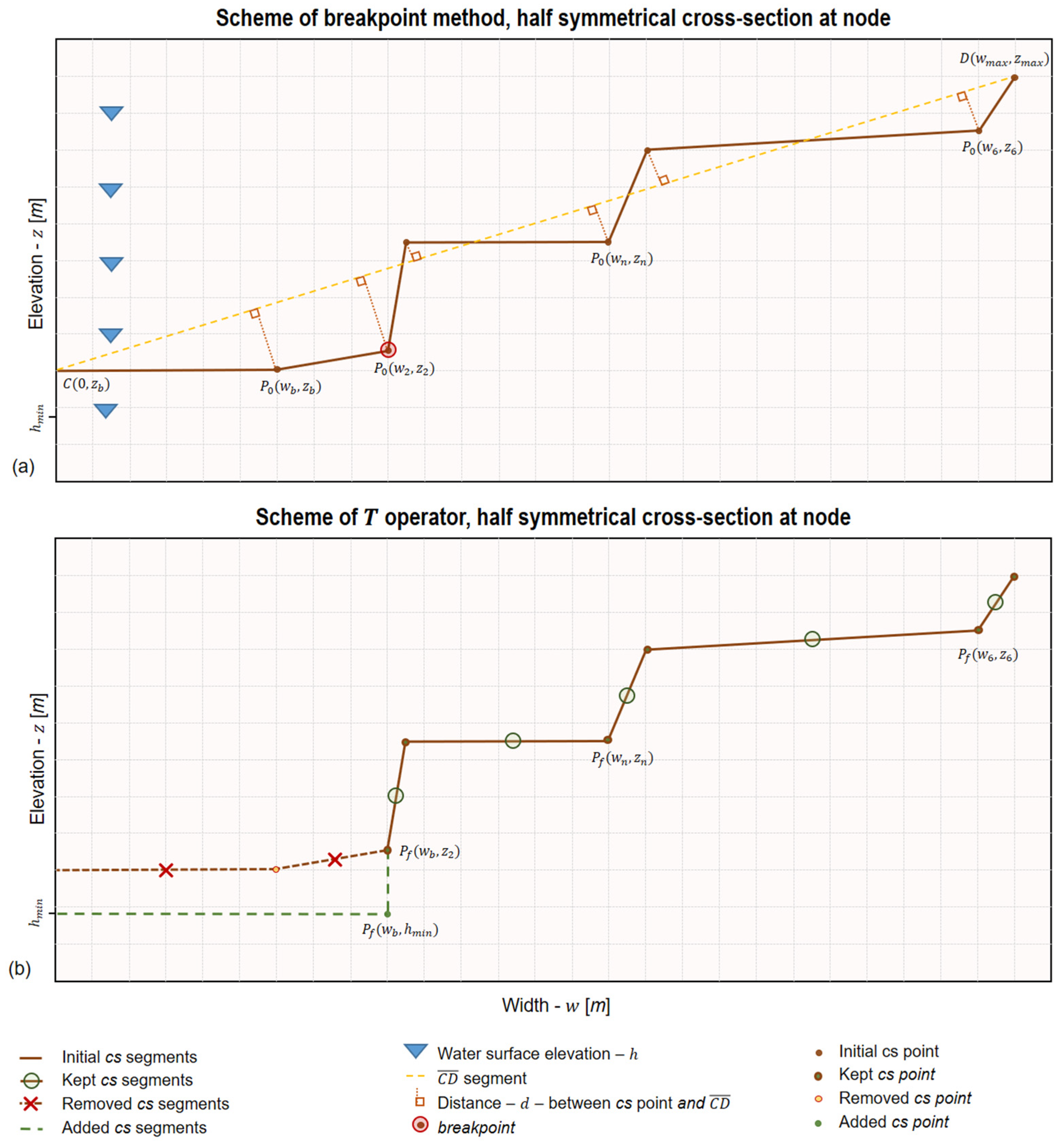
2.2.1. The Breakpoint Method

The slope-break method identifies regions in the cross-section that accommodate different types of hydrological conditions, e.g., low versus high flows. The researchers diverge on how to define these regions [6,7,9]. In our approach, the breakpoint method, we consider the first point selected in the algorithm used to simplify the cross-section profiles [35]. This procedure is shown in Figure 3a.

Consider the symmetrical profile formed by the segments connecting the points $P_0\left(w_n,z_n\right),\forall n\in \left[1,2,\dots ,N\right]$. We create a segment $\overline{CD},C\left(0,z_b\right) \mathrm{a}\mathrm{n}\mathrm{d} D(w_{max},z_{max})$. We compute the orthogonal distance from each point $P_0$ to $\overline{CD}$, $d\left(w_n,z_n\right)$. The breakpoint $P_0\left(w_{n^{\ast }},z_{n^{\ast }}\right)$ is defined as the most distant point from the segment. In Figure 3a, $P_0\left(w_{n^{\ast }},z_{n^{\ast }}\right)=P_0\left(w_2,z_2\right)$. From the defined breakpoint width ($w_{n^{\ast }}$), we add a rectangular channel until $h_{min}$. This is shown in Figure 3b and is performed by the $T$ burning operator.

The $T$ operator is responsible for the modification of the cross-section shape function $w\left(x_j,z\right)$, using a bottom width $\left(w_b\right)$ and a final bottom elevation $\left(z_{b_f}\right)$, $T(w\left(x_j,z\right),w_b,z_{b_f}$). For a given $w_b$, the operator first defines $z_b$, the elevation that corresponds to this width in the original profile (intersection of a vertical line drawn at $w_b$ in the $z\times w$ coordinate system). The operator discards the part of the cross-section located under $z_b$ and keeps the part above it (kept and removed segments in Figure 3b). Then, the operator burns a rectangular channel in the profile. The base of the rectangle is $w_b$ while the height is $z_b-z_{b_f}$ (added segments in Figure 3b).

Being a purely geometrical approach at the node level, the breakpoint method can cause sudden variations in the computed wet area and hydraulic radius along the river stretch. For given water surface elevations at a time instance, this method might create unphysical variations in the computed discharge in short distances.

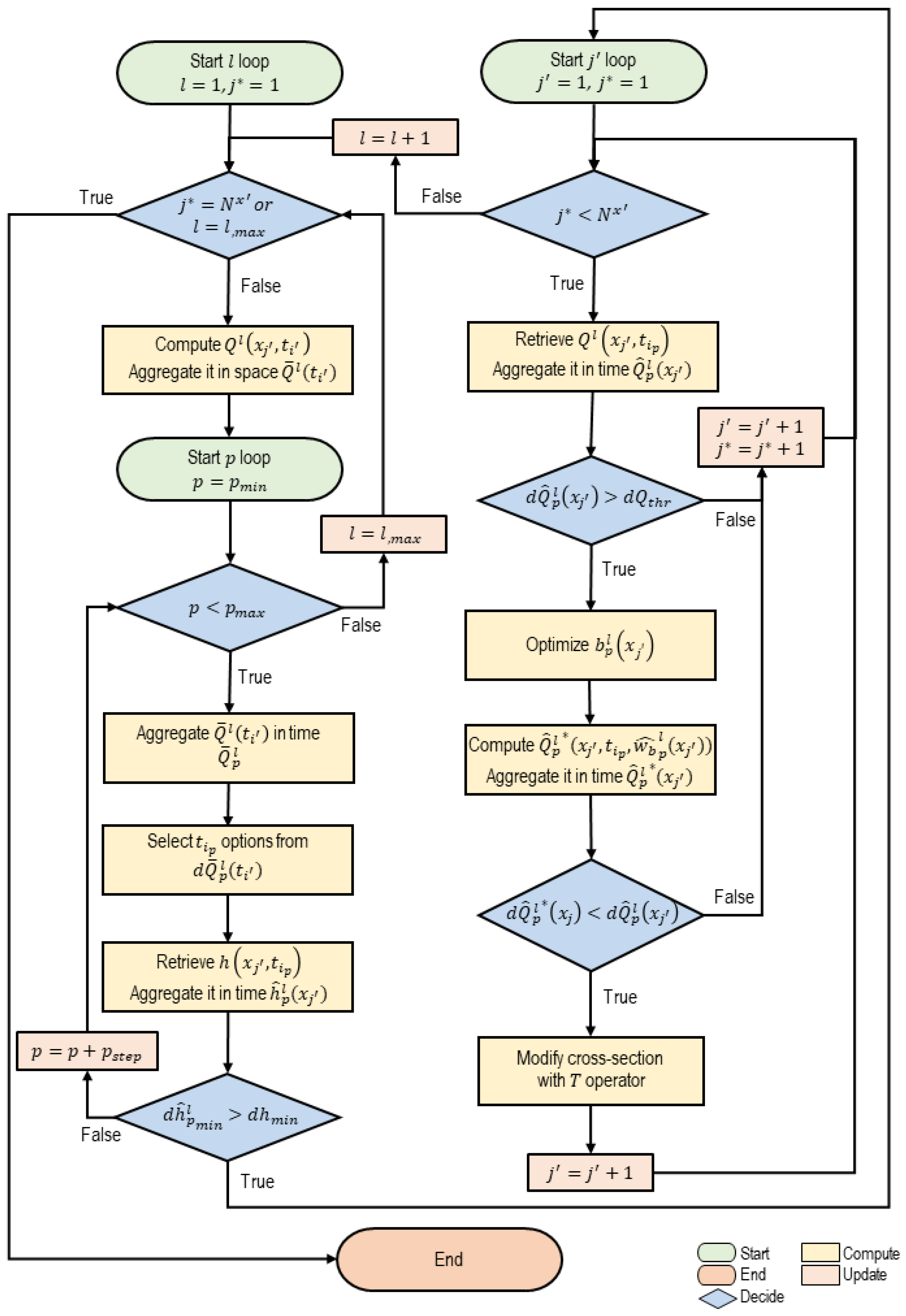
2.2.2. The Continuity Method

Consider the Gauckler–Manning–Strickler relationship (Equation (1)), where $k_m\left(x\right)$ is the roughness coefficient, $A:=A\left(h\left(x,t\right),w\left(x, z\right)\right), R:=R\left(h\left(x,t\right),w\left(x, z\right)\right)$, the wet area and hydraulic radius, respectively, for $z\in [z_b\left(x\right),h_{max}\left(x\right)]$, and $S_f\left(x,t\right)=-\partial h\left(x,t\right)/\partial x$ is the friction slope, which can be approximated as the water surface elevation slope [37,38].

$$Q=k_m A R^{2/3} S_f$$

(1)

Given the dependencies, one can notice that Equation (1) can be expressed as a function of the water surface elevation $\left(h\left(x,t\right)\right)$, the cross-section shape function $\left(w\left(x, z\right)\right)$, the friction slope, and the roughness coefficient, which is assumed constant for the reach:

$$Q\left(x,t\right)=Q\left(k_m, h\left(x,t\right),w\left(x, z\right),S_f\left(x,t\right)\right),\forall z\in \left[z_b\left(x\right),z_{max}\left(x\right)\right]$$

(2)

We introduce the continuity method, which modifies the shape of the cross-sections to ensure a (physically meaningful) flow distribution along the river channel for given water surface elevations. At a certain time instance, we assume the flow does not present large variations across a limited number of nodes, defined according to the SWORD reaches, which stretch for about 10 km.

The continuity method iteratively modifies the width shape function to accommodate a target flow $\left(Q_{target}\right)$. Preference is given to low flows, closer to the bottom of the css, to avoid modifications in the top parts, assuming they are well-represented in the DEMs. The method permits controlled variations in discharge $\left(d{Q}_{thr}\right)$, accommodating natural fluctuations. When variations exceed this threshold, the approach adjusts the width of a rectangular-shaped cross-section with base $b\left(x\right)$ to achieve $Q_{target}$, minimizing discrepancies between computed and target discharges:

$$\widehat{b}\left(x\right)=\underset{b}{\mathrm{arg\; min}}{\left(Q\left(k_m, \overline{h}\left(x\right),b\left(x\right),{\overline{S}}_f\left(x\right)\right)-Q_{target}\right)}^2$$

(3)

where $\overline{h}$ and $\overline{S}$ are averaged values of water surface elevation and slope. To mitigate potential errors in $h$ observations, we utilize an ensemble of time instances (see Appendix A). The methodology ensures continuity through a three-step procedure involving different data subsets and conditions. In all steps, we consider only time instances where at least one-third of the nodes have valid observations. The mathematical formulation of the core algorithm and further details on data subsets are provided in Appendix A.

2.3. Discharge Estimation

The discharge ($Q$) is computed using an integrated version of the GMS, given in Equation (4), where $\partial h\left(t\right)=-(h\left(x+\delta x\right)-h\left(x\right))$, assuming a constant $k_m$ throughout the reach. The deduction of the integrated version is explained in more detail in [32].

$$Q\left(t\right)={\displaystyle \frac{k_m{\left(\partial h\left(t\right)\right)}^{1/2}}{{\left({\int }_x^{x+\delta x}{A\left(x,t\right)}^{-2}{R\left(x,t\right)}^{-4/3}dx\right)}^{1/2}}}$$

(4)

Solving the discharge would be straightforward if we had full information on the river channel’s bathymetry and roughness coefficient. However, the latter is unknown, and we only have partial information on the bathymetry. We rely on a probabilistic approach to estimate the flow along with these unknown variables. We define possible candidates for the discharge by varying the roughness and the wet bathymetry. The latter is considered to be a rectangular channel defined by the bottom width of the dry bathymetry $\left(w_b\right)$ and variable bottom elevation $\left(\mathrm{z}\prime \right)$ to be estimated. For each pair of $\mathrm{z}\prime \times k_m$ candidates, we compute the mean flow in time, $\bar{Q}\left(\mathrm{z}\prime ,1\right)$, and extract its corresponding probability, $\rho \left(k_m\bar{Q}\left(\mathrm{z}\prime ,1\right)\right)$. The final estimated discharge per time, $\widehat{Q}\left(t\right)$, is given as the weighted mean solution given by the integral:

$$\widehat{Q}\left(t\right)=\underset{k_m^{lb}}{\overset{k_m^{ub}}{\int }}{k}_m\underset{{\mathrm{z}\prime }_m^{ub}}{\overset{{\mathrm{z}\prime }_m^{ub}}{\int }}Q\left(t,\mathrm{z}\prime ,1\right)\rho \left(k_m\bar{Q}\left(\mathrm{z}\prime ,1\right)\right)d\mathrm{z}\prime d{k}_m$$

(5)

To define the integration limits for the roughness Strickler coefficient, we consider a wide range of values, from 10 to 60 $\mathrm{s}/{\mathrm{m}}^{1/3}$, which covers the values expected for natural river channels [39,40]. The bounds for the wet bathymetry are defined according to the prior mean discharge by inverting the traditional GMS, similar to what is performed in the continuity approach (Equation (3)), but solving for the height instead of the width. For each bound, the target discharges are taken from the prior probability distribution, and the roughness coefficient is defined accordingly to match the lower or upper limits. The ensemble of times is selected according to the proximity to the dry bathymetry’s mean discharge.

After obtaining the discharge from Equation (5), the output roughness is picked from the candidates as the one with the lowest root mean square error compared to the discharge output. The final depths are resolved with the same inversion to compute the integration limits for the wet bathymetry. Here, we use low-flow times instead of mean times and a target discharge from the discharge output, not the prior distribution.

The output cross-sections correspond to the third blue box in Figure 1 and the blue dotted lines in Figure 2. With the keep run for the cross-section pre-processing, the probabilistic approach (Equation (5)) does not consider candidates for the bottom elevation, assuming the cross-section provided is correct.

2.4. Evaluation Metrics

The metrics Relative Root Mean Squared Error (RRMSE), percent bias (PBIAS), Pearson correlation (cor), Kling–Gupta efficiency (KGE), and KGEα (ratio of variances) are used as indicators of errors. The concept of relative is frequently employed; in these cases, the error metric is divided by the validation mean. In some parts, the data are filtered into five flow categories according to the cumulative probability distribution of the validation discharge ($Q_{val}$). Minimum flows have $Q_{val}$ smaller than 5%; for low flows $5\%\le Q_{val}<25\%$; mean flows; $25\%\le Q_{val}<75\%$; high flows $75\%\le Q_{val}<95\%$; and maximum flows have $Q_{val}\ge 95\%$.

3. Datasets

All data mentioned is openly available and listed in the Open Data section.

3.1. Global Remotely Sensed Digital Elevation Models (DEMs)

Over the past 25 years, distinct organizations have contributed to creating global DEMs.

Table 1. Summary of (quasi-)global digital elevation models.

DEM	Version	Features	Pixel Size	Main Source	Acquisition Period	Accuracy	Dataset Reference
SRTM	3.0	DSM	1″	C band SAR	February 2000 (11 days)	<9 m (LE90) [41]	[42]
ASTER	3.0	DSM	1″	Stereo NIR imagery	2000–2013	8.5 m (RMSE) [43]	[44]
TanDEM-X	1.0	DSM	3″	X band SAR	2011–2015	<10 m (CE90) [45]	[46]
AW3D30	4.0	DSM	1″	Stereo PAN imagery	2006–2011	<6 m (LE90) [47]	[48]
MERIT	1.0.3	DSM *	3″	Modified SRTM	February 2000 (11 days)	<12 m (LE90) [49]	[49]
MERIT-Hydro	1.0.1	DSM *	3″	Modified SRTM	February 2000 (11 days)	-	[50]
Copernicus	2022_1	DSM	1″	Modified Tandem-X	2011–2015	<3 m (LE90) [51]	[24]
NASADEM	1.0	DSM	1″	Reprocessed C band SAR	February 2000 (11 days)	-	[52]
FABDEM	1.2	DTM	1″	Modified Tandem-X	2011–2015	<9 m (90%) [53]	[54]

* Even though the vegetation cover was removed, MERIT and MERIT Hydro are not considered DTMs as they still represent the heights of buildings.

summarizes the (quasi) global models analyzed in this study, all of which are openly available for research purposes.

The heights represent natural and/or anthropological features of the environment (Digital Surface Models—DSMs) or the elevation of the “bare Earth” (Digital Terrain Models—DTMs). The vertical accuracy given in Table 1 corresponds to the metrics provided by the data producers or systematic validation studies. To our knowledge, these are not available for MERIT-Hydro or NASADEM.

In the column “main source” of Table 1, the models can be divided into those directly derived from remotely sensed images and those built on top of one of the existing DEMs with added processing steps.

In the first group, SAR interferometry (InSAR) was used to retrieve the heights for SRTM [55], NASADEM [56], and Tandem-X [57], while ASTER [58] and AW3D30 [59] employed stereocorrelation. InSAR limitations include (i) smooth terrain or water surfaces, where little of the emitted signal returns; (ii) dense vegetation, urban areas, or fast-moving water bodies, which can lead to a lack of coherence [60,61,62]. Stereocorrelation has limitations over dense vegetation and water surfaces, which can confuse the matching process as they lack distinct features [63,64,65,66,67,68]. The public version of Tandem-X DEM analyzed in this study has no further refinement [69], while the aforementioned products were post-processed to detect anomalies and fill voids.

The second group comprises four DEMs. The “Multi-Error-Removed Improved-Terrain” (MERIT) DEM was built by removing errors in the models SRTM and AW3D30 [49]. MERIT-Hydro is the hydrologically adjusted version of the MERIT DEM, built using auxiliary water datasets [50]. Copernicus DEM [70] is a resampling from WorldDEM^TM [71], which was, in turn, built from TanDEM-X. The “Forest And Buildings Removed Copernicus DEM” (FABDEM) modified the ESA DEM and turned it into the only DTM analyzed in this research [53].

Both InSAR and stereocorrelation are limited in retrieving elevation over water. Overcoming this, most of the global DEMs were refined by modifying the water bodies. The post-processing of SRTM [72], ASTER [73], and WorldDEM^TM [71] included a stepwise adjustment of the height of rivers from a point upstream to the sea, whose height is set to zero. To detect rivers, the first and the last one employed a minimum width criteria of 183 and 50 m, respectively. For ASTER, there was a minimum area of 0.2 km² for the detection of rivers or lakes. The size of the step of the first two is one meter, as opposed to 0.5 m for the last DEM. Along the river length, the breakpoints of the steps are a result of extensive iterations. After the correction of the heights of the water bodies, the riverbanks were lifted by one meter for ASTER and SRTM and to at least the height of the neighboring water body in WorldDEM^TM.

A core motivation for reprocessing SRTM data for the NASADEM was improving the water representation [74]. The adjustments were mainly focused on a better agreement between the adjacent terrain and the interpolated river heights. However, the authors mention that the monotonicity of the river that is present in SRTM might have been lost in some locations. As with SRTM, there was a step to ensure the banks were at least one meter higher.

For Copernicus DEM [70] and FABDEM [53], there is no mention of any extra procedures for the water bodies. According to the producers of the Copernicus DEM, the resampling made from WorldDEM^TM does not necessarily keep the hydrological consistency of the original DEM.

The authors of MERIT mention the improvement in the elevation representation of floodplains, yet no additional procedure was indicated for water bodies [49]. The producers of MERIT-Hydro used auxiliary water masks to create a likelihood mask to burn the water bodies on the DEM [50]. After properly defining the streams, the terrain was modified to enforce the desired flow direction. The river heights were modified so they are always decreasing. For AW3D30, the water surfaces were interpolated from neighboring valid pixels without further refinement [75].

3.2. Water Surface Elevation from Virtual Stations

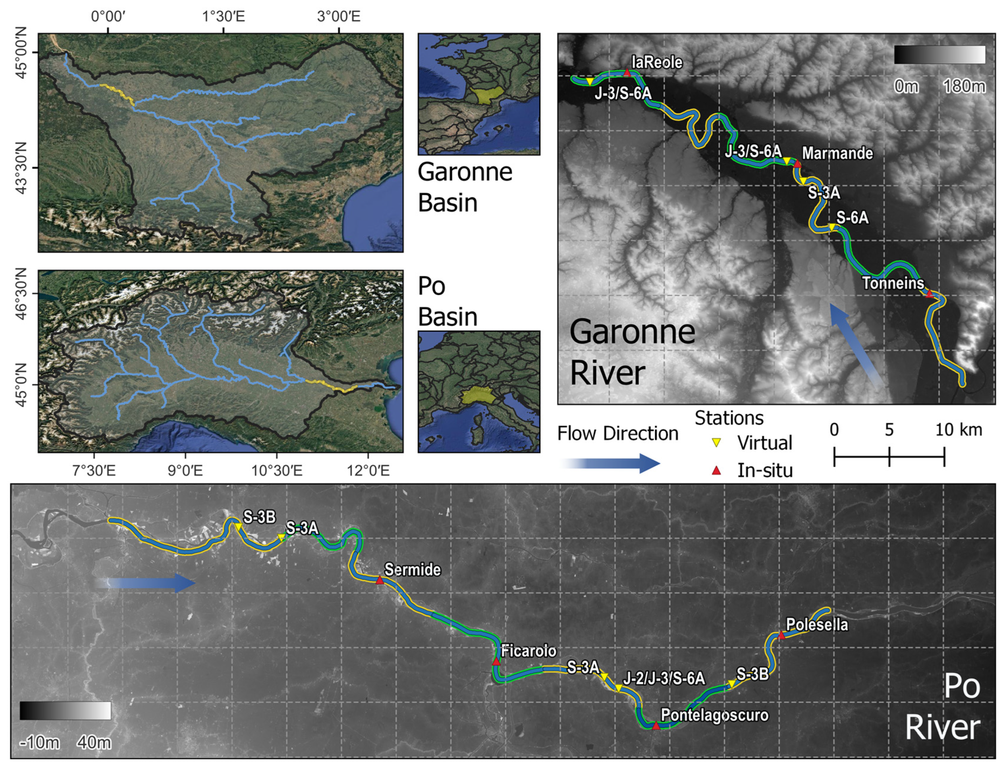
Since the early 1990s, satellite radar altimetry has enabled continuous monitoring of water surface topography by measuring the round-trip travel time of electromagnetic pulses emitted in the nadir direction. The returned signals, recorded as waveforms, are processed using retracking algorithms to determine the distance between the satellite and the water surface, with corrections for atmospheric and geophysical effects [76]. Originally designed for ocean height measurement, altimetry is also applied to lakes and rivers at “virtual stations”, where ground tracks intersect water bodies. Unlike oceans, inland water bodies produce complex waveforms due to mixed reflections, often requiring empirical models for accurate retrieval [77].

Early studies for rivers were focused on large river basins, with river widths greater than 1 km, due to the footprint size of the satellites available at the time (e.g., ERS1 and TOPEX/Poseidon [78,79]. Nowadays, with more suitable retracking algorithms and modes [80,81] and the use of SAR-like processing in newer sensors (e.g., Sentinel-3 and Sentinel-6 [82,83]), nadir altimeters can resolve water surface elevation $\left(h\right)$ for rivers in the orders of a few hundred meters in width. Some limitations of discharge modeling from radar altimetry can be connected to narrower channels and more mixed signals in the waveform [14].

Different organizations provide inland altimetry time series: DAHITI [84,85], G-REALM [86], Hydroweb.next [87], and Hydrosat [88]. In this study, we obtained data from Hydroweb.next.

The beginning of the study period of this research was defined according to the year Jason-3 and Sentinel-3A were launched: 2016. The end of the study was mid-2024. During this period, the following traditional altimetry satellite missions orbited the Earth: Jason-2, Jason-3, Sentinel-3 (A and B), and Sentinel-6.

Jason-2 was launched in 2008 and remained operational until mid-2016, when it was replaced by its successor, Jason-3. Both satellites operate with a 9.96-day repeat cycle and are equipped with conventional low-resolution mode radar altimeters [89,90]. Overland, the footprint of these sensors is in the order of a few kilometers; the exact value depends on the slope of the surface and large-scale roughness.

Each Sentinel-3 is equipped with a Synthetic Aperture Radar Altimeter (SRAL) and has a revisit time of 27 days [82]. Sentinel-3A was launched in 2016, while Sentinel-3B was launched in 2018. These sensors’ spatial resolution is much higher than that of conventional altimeters, around ~300 m [77].

Launched in 2020, Sentinel-6’s payload allows both SAR capabilities and the conventional mode of acquisition, as with Jason-3 [83]. From April 2022, Sentinel-6 took the position previously occupied by Jason-3.

4. Study Areas

Figure 4 displays the two study areas: the Garonne River in France and the Po River in Italy. They were selected due to the availability of comprehensive bathymetric reference data covering both underwater and above-water surfaces.

4.1. The Garonne River

The Garonne runs 525 km from the Pyrenees to the Gironde estuary. The reaches analyzed in this study are in the “middle Garonne”, a region characterized by strong floods, under the combined influence of the tributary rivers Tarn and Lot [91]. The lowest flows are observed in the late summer months (August–September), from which the discharge gradually increases, reaching the peak in January–February [92]. In Tonneins, the mean discharge in our study period was 490 m³/s, ranging from 60 m³/s to 6000 m³/s.

The part of the river under consideration in this study is shown in the top right part of Figure 4. It corresponds to six SWORD reaches. The widths corresponding to their mean flow, extracted from GRWL, vary from 150 to 190 m.

The data for the three in situ stations in the Garonne River can be accessed in EauFrance HydroPortail. We downloaded instantaneous measurements of water surface elevation and discharge. The interval between the collection times is 15 min, but some gaps exist. We analyzed the time series visually to detect outliers. The data were then aggregated to daily means, and the $h$ was corrected to refer to the geoid EGM08 model. Unless specified otherwise, the validation of the discharge was conducted within the reach of Tonneins.

The satellite missions Sentinel-3 (A and B), Jason-3, and Sentinel-6A fly over this study area (respectively, S-3A, S-3B, J-3, and S-6A in Figure 4). In this study, we obtained data from four virtual stations in Hydroweb.next, their locations are illustrated in Figure 4, with the respective mission. In this database, their identifiers are, from upstream to downstream: “KM201”, “KM0194”, “KM0191”, and “KM0163”. Between June 2016 and June 2024, there are a total of 376 measurements from Jason-3, 103 from Sentinel-3, and 167 from Sentinel-6. No further processing (e.g., removal of outliers or smoothing) was performed.

Between 2021 and 2026, the French National Institute of Geographic and Forest Information is working to provide DEMs acquired by aerial LiDAR (Airborne Light Detection and Ranging) surveys [93]. In 2013, an Acoustic Doppler Current Profiler (ADCP) obtained the underwater topography at defined points of the river. Our study area has twenty-seven surveyed cross-sections. The combination of these data was performed by Centre Européen de Recherche et de Formation Avancée en Calcul Scientifique (CERFACS).

4.2. The Po River

The Po River flows from the Alps towards the Adriatic Sea for about 650 km. A levee system extends for the last 420 km of the river watercourse [94]. In its alluvial plain, the Po Valley, the river follows a pluvial regime with two peak periods, one in the autumn, which reflects the intensification of rainfall, and another in the spring, corresponding to the snowmelt, while the lowest flows are observed in the summer months (July–August) [95]. In our study period, the mean discharge at Sermide was 1200 m³/s, ranging from 160 m³/s to 6000 m³/s.

Figure 4 illustrates the seven SWORD river reaches analyzed in this study. Their mean flow widths range from 280 to 480 m.

The data for the four in situ stations in the Po River is provided by Arpae-Simc Emilia-Romagna. We downloaded $h$ and $Q$ data. The interval of collection was 30 min; gaps are also present in this dataset. The data were preprocessed in the same way as with the Garonne River. Unless specified otherwise, discharge validation efforts were focused on the reach where the station Sermide is located.

These reaches are in the path of the same satellite missions as the Garonne study area, with the addition of Jason-2 (J-2 in Figure 4). In this study, we obtained data from five virtual stations from Hydroweb.next: “KM0145”, “KM0140”, “KM098”, “KM096”, and “KM082” from upstream to downstream (Figure 4). In the study period, there are a total of 206, 275, 18, and 15 measurements from J-3, S-3, S-6, and J-2, respectively.

The Po River Basin Authority produced a 2 m resolution DEM in 2005, offering detailed information on the riverbed topography across the middle-lower section of the watercourse [96]. This DEM integrates data acquired by aerial LiDAR and multibeam sonar at defined cross-sections. Eighty surveyed cross-sections are present in the study area.

5. Results

The results are separated into four sections. The first section focuses on the comparison between the DEMs and the LiDAR in the entire study area, considering only the dry bathymetry. The second section explores how the choice of DEM and the burning methods influence the discharge outputs using $h$ data from in situ stations. A total of 80 test cases were analyzed. In the third section, we study how changing the h source to virtual stations modifies the discharge estimates. In the fourth part, the focus is then shifted to the full bathymetry, comparing the effective output geometry in hydraulic terms for the whole study area.

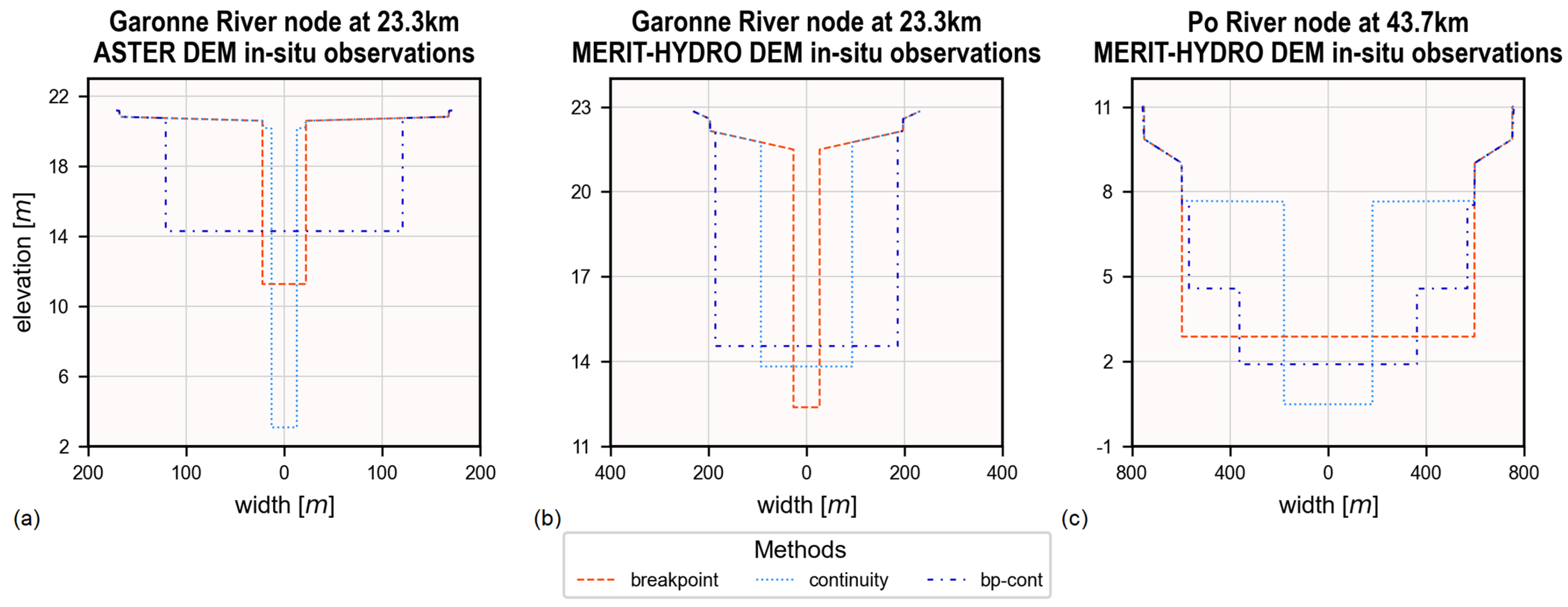
5.1. Impact of DEMs on the Dry Bathymetry

For the cross-sections’ top elevation, there is an overall agreement between the DEMs and the LiDAR. Dikes, riparian vegetation, and buildings can cause small variations. The LiDAR depth is typically lower than other DEMs. The bottom depth of the LiDAR reference for the Po shows more variations than the one of the Garonne River.

In both study areas, the post-processing stepwise procedure to decrease the water surface elevation can be observed in the SRTM, ASTER, NASADEM, Copernicus, and FABDEM. Some sinks happen because of nearby water bodies whose height was not modified. In the first 35 km of the Garonne River for ASTER, the stepwise procedure resulted in values higher than those of the adjacent terrain. Our methodology for defining and extracting the cross-section does not expect the water level to be higher, showing a shallow, narrow channel that is relatively higher (Figure 5a).

The bottom profiles of AW3D30, and especially Tandem-X, present more variations. The first has interpolation-related inconsistencies, and the last lacks special treatment for water bodies. Overall, MERIT and MERIT-Hydro exhibit higher bottom elevations, which are illustrated in the representative cross-sections (Figure 5). This is attributed to their resolution (90 m) and the width of the rivers, which increase the likelihood of capturing mixed targets (water and land).

To analyze the dry bathymetry, we focus on the common part between the LiDAR’s reference and the global DEMs. The results are presented in

Table 2. Common Depth and Relative Errors in Area.

River	DEM	Common Depth with Reference (%)			Relative Errors in Area for Common Part (%)
		25%	Median	75%	25%	Median	75%
Garonne	AW3D30	24.79	38.80	54.16	−61.73	−42.18	−28.38
	ASTER	23.85	31.50	44.68	−37.66	−16.74	−1.49
	SRTM	28.80	35.03	45.58	−40.39	−28.95	−15.62
	NASADEM	44.74	54.47	62.99	−29.90	−17.45	−7.26
	MERIT	16.96	23.39	32.26	−48.27	−26.08	−15.52
	MERIT-HYDRO	22.53	28.98	37.49	−30.43	−16.95	−7.79
	TANDEM-X	26.82	40.64	58.80	−56.66	−34.39	−20.53
	COPERNICUS	81.27	91.08	100.00	−4.71	3.40	9.64
	FABDEM	80.71	90.47	100.00	−7.55	−0.25	7.73
Po	AW3D30	35.53	46.03	57.79	−33.41	−21.31	−13.73
	ASTER	48.28	57.26	65.35	−16.64	−6.21	−0.23
	SRTM	46.43	54.45	62.81	−11.72	−5.07	0.81
	NASADEM	43.78	54.03	61.09	−15.75	−7.23	−1.75
	MERIT	28.40	35.55	41.45	−37.51	−23.28	−14.22
	MERIT-HYDRO	33.97	40.42	46.89	−32.56	−21.28	−12.18
	TANDEM-X	34.77	51.23	75.02	−60.17	−41.04	−25.31
	COPERNICUS	50.26	58.92	66.32	−8.82	−3.53	0.10
	FABDEM	48.00	56.51	64.52	−9.21	−4.18	0.14

. For each node, we first determine the lowest top elevation ($z_{{max}_c}\left(x_j\right)$) between the DEM under analysis and the reference. The cross-sections’ top is then cropped to this common height. The common depths with the LiDAR (Table 2) are then computed as:

$$\left(z_{{max}_c}\left(x_j\right)-z_{b_{DEM}}\left(x_j\right)\right)/\left(z_{{max}_c}\left(x_j\right)-z_{b_{ref}}\left(x_j\right)\right)$$

where $z_b$ is the bottom elevation of the cross-section. In the node located at 43.7 km in the Po River for FABDEM (Figure 5b), for example, this value would be $\left(14-4\right)/\left(14-1\right)=77\%$. The values presented in the corresponding columns in Table 2 are aggregated in space. We also analyzed the common area. For this, in addition to cropping to the $z_{{max}_c}\left(x_j\right)$, we also limit the bottom part to the highest elevation between the reference and the target DEM. The area difference is expressed as relative errors in Table 2.

In Table 2, one can see there is an overall tendency to underestimate the area of the dry bathymetry. Except for Tandem-X, Copernicus, and FABDEM, dry bathymetry is better represented in the Po than in the Garonne River, with smaller area underestimations and a larger common observed depth.

For both study areas, the median common depth observed by MERIT and MERIT-Hydro is the smallest compared to the other DEMs. Tandem-X’s and AW3D30’s underestimation of the area is remarkable in both study areas, indicating narrower channels, as seen in the sample cross-section for the Garonne (Figure 5a) and the Po (Figure 5b).

FABDEM and Copernicus stand out with the smaller absolute median errors, with over 50% of the errors within ±10% of the LiDAR in both regions (Table 2). This is particularly relevant as those are also the DEMs with the largest common depth. These DEMs have a strikingly high common depth with the reference for the Garonne. With a limited number of sampled locations and depth similar to these DEMs, the validation with the Garonne’s LiDAR bathymetry must be performed mindfully.

5.2. Impact of DEMs and Cross-Section Burning on the Discharge Estimate

In this section, the results presented correspond to the runs with in situ water surface elevations $\left(h\right)$. In the keep run, the depth and the width of the cross-sections (cs) are not modified. This method limits the number of time instances and nodes with outputs, as only $h$ observations inside the original css are considered.

In the keep run with the reference DEM (LiDAR), the estimated discharge for the Po River is almost a perfect fit (Figure 6b). It captures perfectly the flow dynamics (cor = 1.0), with a slight overestimation of the flows (PBIAS = 2.25%). Even with the $h$ interpolation and constant roughness, the model achieves outstanding performance.

For the Garonne River (Figure 6a), the dynamics are captured very well (cor = 0.99), but it exhibits a significant overestimation of flows (PBIAS = 31.65%), particularly at lower values. The absence of low flows (<250 m³/s) and a bottom depth that is similar to other DEMs (Table 2) suggests the lower number of surveyed cross-sections and the interpolation between them significantly influences the results. By modeling only nodes close to the surveyed sections, the estimated discharge suffers from a strong underestimation (PBIAS = −59.4%), and the low flows are constantly close to zero. This indicates the $h$ interpolation between the in situ stations and constant roughness also degrade the results for the French River.

In many cases of the keep run with the other DEMs, the discharge could not be estimated due to insufficient dates. This run generally results in inferior outcomes, as shown in the smaller KGE bars of Figure 7. Applying any of the burning methods to the symmetrical css results in KGEs closer to 1.0, the ideal value, highlighting the importance of this study.

In the keep run for the Garonne River, Copernicus and FABDEM unexpectedly outperform the LiDAR (Figure 7a); however, they underestimate the flows (PBIAS ≈ −22.45%). The good results of these elevation models are linked to their high observed depths (Table 2), which dropped the need for cross-section preprocessing.

The errors decrease when one of the burning methods is applied: breakpoint, continuity, or bp-cont (Figure 7). Overall, the Po River’s results tend to be better than those of the Garonne. With the preprocessing, most runs effectively capture flow dynamics, with cor ≥ 0.95. Exceptions occur with ASTER and MERIT-Hydro for the Garonne using the breakpoint method, where this coefficient drops to 0.81 and 0.74, respectively. ASTER’s results improve with the continuity method (cor = 0.93).

With the breakpoint method in the Garonne River, MERIT-Hydro and ASTER underperform (Figure 7a), with KGE values below 0.1, while Copernicus and FABDEM deliver exceptional results. This method performs notably better for the Po River (Figure 7b), where the breakpoint method achieves KGE > 0.65 for all DEMs except Tandem-X. Performance issues with Tandem-X stem from variability in dry bathymetry (Table 2), which is related to insufficient processing. Inconsistencies in this part of the bathymetry with AW3D30 for the French River also diminish the predictability of the discharge model for this DEM.

The continuity method degrades the estimates’ performance in the Po River for AW3D30, MERIT, and MERIT-Hydro, with KGE reductions of at least 0.25 compared to the breakpoint method (Figure 7). With this approach, Copernicus and FABDEM reach high KGEs (>0.86) in both rivers, reflecting their superior representation of dry bathymetry and high observed depths (Table 2).

The bp-cont method results in correlation coefficients consistently exceeding 0.99, absolute bias remaining below 15%, and KGE always above 0.62. This method outperforms others in 15 out of 18 variations (Figure 7), showcasing its adaptability.

In the relatively worse bad cases for the bp-cont technique (Copernicus and FABDEM for the Po), there was an increase in KGEα (~1.25). Further, the model tends to slightly overestimate the flows (PBIAS = 8%), independent of the flow patterns. The higher KGEα and the PBIAS reflect a wider bottom of the output cross-sections.

To better illustrate the outputs of the burning methods, hydrographs are presented for the ASTER in the Garonne (Figure 8a), MERIT-Hydro in the Garonne (Figure 8b), and Po (Figure 8c). Representative css for each of these cases are displayed in Figure 9.

MERIT’s and MERIT-Hydro’s performance is impacted by the low depth common depth with the LiDAR in the dry bathymetry (Table 2). In the Garonne, the breakpoints retrieved for the latter DEM are usually quite high, resulting in deep, narrow squared channels (Figure 9b), which are only able to capture very low flows (Figure 8b). High peaks, such as the one of January 2022, are properly modeled when the observed water surface elevations are within the dry bathymetry from the DEMs, e.g., above 22 m in the node represented in Figure 9b.

The narrow, deep channel is also seen in many nodes in the ASTER DEM for the Garonne with the breakpoint method (Figure 9a). As explained in Section 5.1, this channel originates from a relatively more elevated water body than the surroundings. As with MERIT-Hydro, the narrow channel of ASTER limits the model’s ability to predict higher flows (Figure 8a). The wider cross-section reconstructed in some nodes improves the results compared to MERIT-Hydro.

For the Garonne River, ASTER (Figure 8a) performs even worse with the continuity method (KGE < 0) due to the persistence of narrow channels (Figure 9a). On the other hand, MERIT-Hydro shows some improvement (Figure 8b). In the first step of this method, the time instances in which at least ⅓ of the nodes have valid observations inside the original symmetrical css are considered. Due to the high narrow channels seen in the original ASTER but not in MERIT-Hydro (Figure 5a), the continuity assumption propagates the error and further degrades the results for the first DEM but not for the latter.

An interesting anomaly is observed in the Po with MERIT-Hydro during the July 2022 drought (Figure 8c). A non-physical increase in discharge at low flows is noted for the continuity method but not for the others. This is attributed to the GMS equation (Equation (1)) with relatively narrow rectangular channels with very low water levels (Figure 9c).

The bp-cont method combines the strengths of the other methodologies. Particularly for the MERIT-Hydro in the Po, this approach frequently defines two regions with distinct widths (Figure 9c). The highest width is derived from the breakpoint and the first part of the continuity method, while the lowest is derived from the sequential parts of this algorithm. Dividing the regions allows better accommodation of distinct flow conditions (Figure 8c), resulting in a very good KGE (Figure 7b).

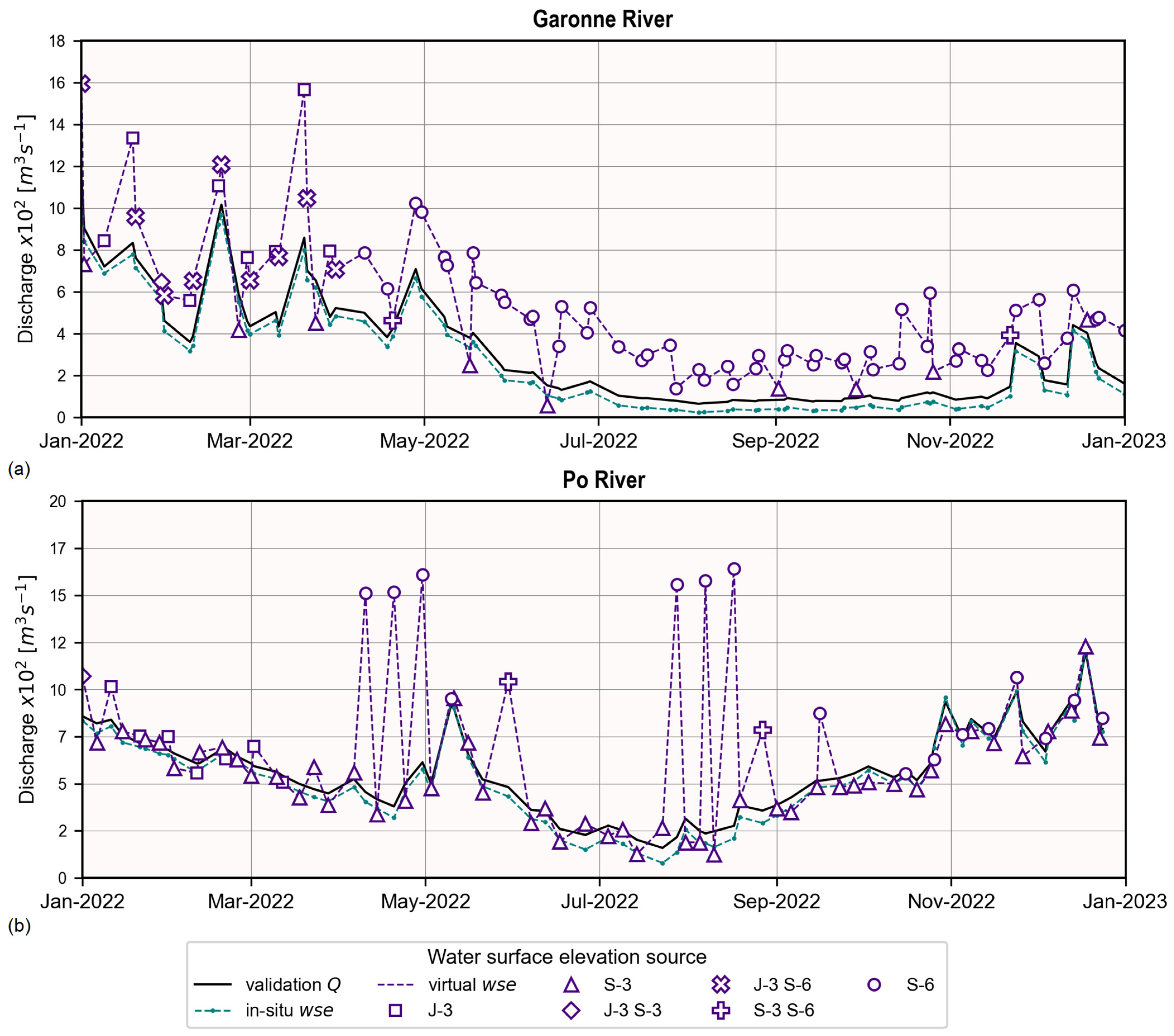
5.3. Impact of Water Surface Elevation Sources on the Discharge Estimate

When remotely sensed (RS) water surface elevation $\left(h\right)$ data are used, there is a general decline in performance. The uncertainties RS $h$ decreased the correlation coefficients by approximately 0.14 for the Garonne and 0.12 for the Po, with the resulting values ranging from 0.84 to 0.88. In the Garonne, the bias metrics also reveal critical differences, with a significant shift from underestimation (–∼15%) to overestimation (∼30%). For the Po, such shifts were not observed.

In the Italian river, the bp-cont method produces KGEs above 0.73 in all the DEMs except AW3D30, with KGE = 0.58. The model was very good for ASTER, SRTM, NASADEM, MERIT, and MERIT-Hydro (KGE ≈ 0.85). The decreased performance compared to the in situ $h$ follows the change in the correlation coefficient. In this river, AW3D30, Copernicus, and FABDEM had the best results with the breakpoint method (KGE ≥ 0.85), which is similar to the runs with in situ elevations (Figure 7b).

In the French river, the results are more limited. ASTER, AW3D30, NASADEM, and FABDEM have 0.63 ≤ KGE ≤ 0.72 for the bp-cont approach. The other DEMs have KGEα > 1.3 and a larger PBIAS (∼42%), resulting in KGEs 0.38 ≤ KGE ≤ 0.46.

The continuity method failed to find solutions for some DEMs for the Garonne (SRTM, MERIT, and MERIT-Hydro). This was primarily due to a lack of valid observations inside the original cross-sections for at least one-third of the nodes. The virtual stations reduced the probability of finding points that would fit these more elevated and shallower css (Table 2).

To further explore the differences in the output discharge when we move from in situ to remotely sensed water surface elevations, we focus on the breakpoint technique. Based exclusively on geometric considerations, the cross-sections derived from this method are similar for both $h$ sources before the discharge estimation part. Thus, any differences in the results are mostly due to the variation in the $h$ data, which influences the final discharge estimation step.

Interestingly, the breakpoint method for Copernicus DEM for the Garonne shows dramatic differences: the KGE decreases from 0.88 (in situ) to 0.51 (virtual). This deterioration can be attributed to errors introduced by the constant slope and the water surface elevation source. Comparing these to the modeled discharge, there is a weaker correlation with the slope errors (=0.4) and a stronger one (>0.8) for the mean $h$ errors, emphasizing the influence of the latter’s accuracy.

Table 3. Discharge error indicators by flow and sensor for the Copernicus DEM and the breakpoint method.

River	Flow	Date Distribution		RRMSE						PBIAS
		In Situ	All	In Situ	J-2	J-3	S-3	S-6	All	In Situ	J-2	J-3	S-3	S-6	All
Garonne	Min	4.98%	6.15%	55.45%	nd = 0	138.51%	nd = 4	242.42%	228.45%	−55.44%	nd = 0	120.25%	nd = 4	232.14%	213.40%
	Low	19.99%	23.26%	38.89%	nd = 0	131.61%	81.41%	126.83%	181.08%	−38.82%	nd = 0	121.35%	39.79%	119.36%	145.96%
	Mean	50.02%	53.49%	10.96%	nd = 0	64.64%	35.87%	74.86%	106.22%	−10.68%	nd = 0	57.70%	−30.29%	70.24%	48.51%
	High	19.99%	16.45%	5.21%	nd = 0	33.43%	28.39%	39.69%	40.14%	−5.05%	nd = 0	25.96%	−20.65%	36.22%	27.53%
	Max	5.01%	0.66%	5.62%	nd = 0	nd = 1	nd = 2	nd = 1	nd = 4	−2.13%	nd = 0	nd = 1	nd = 2	nd = 1	nd = 4
	All	100.00%	100.00%	9.97%	nd = 0	58.83%	49.51%	71.66%	60.38%	−8.97%	nd = 0	42.12%	−12.99%	66.04%	38.09%
Po	Min	5.02%	5.11%	21.09%	nd = 0	nd = 0	44.69%	nd = 5	241.29%	−20.80%	nd = 0	nd = 0	−0.62%	nd = 5	143.75%
	Low	19.98%	22.38%	11.73%	nd = 3	41.68%	36.42%	nd = 7	34.54%	4.62%	nd = 3	3.29%	14.43%	nd = 7	8.14%
	Mean	50.00%	48.42%	6.61%	nd = 5	19.29%	7.52%	nd = 6	14.26%	6.16%	nd = 5	10.95%	−3.49%	nd = 6	2.36%
	High	19.98%	20.68%	3.61%	nd = 6	9.86%	10.80%	nd = 0	5.17%	1.62%	nd = 6	0.65%	−5.85%	nd = 0	−0.80%
	Max	5.02%	3.41%	4.41%	nd = 1	nd = 5	nd = 8	nd = 0	16.12%	2.02%	nd = 1	nd = 5	nd = 8	nd = 0	−6.58%
	All	100.00%	100.00%	6.57%	11.03%	29.24%	21.67%	124.24%	26.23%	3.64%	2.93%	6.97%	−2.35%	84.10%	3.23%

, segmented by sensors and flow types, further explores the variation in the $h$ source for the breakpoint method for Copernicus DEM. As the number of samples for each flow category is not uniform, ten random dates were selected from each class to compute the error indicators. If there were not sufficient dates, the cell contains “nd” and the number of dates. The indicators for the “all” rows use all available dates.

Minimum flows are subject to larger errors with both in situ and in the RS observations. This is expected as the model estimates the discharge, roughness, and bottom depth simultaneously. Therefore, when the $h$s are closer to the lower part of the cross-sections, which was also estimated, the discharge is more prone to errors. However, the magnitude of the errors for the RS data is much larger in the min flow range, with major overestimations.

Analyzing the performance of each sensor (Table 3), Sentinel-3 (S-3) shows better indicators than Jason-3 (J-3) for both rivers. The number of observations for Jason-2 is limited as it was decommissioned just after the study period started. Similarly, fewer observations for Sentinel-6 (S-6) can be attributed to the shorter period this satellite has been in orbit.

For the Garonne River, S-6 has similar metrics to J-3, while S-3 has better indicators, especially considering the absolute bias. For the Po River, the indicators for S-6 are significantly worse than the other sensors. This is aggravated by the absence of observations of high and max flows, which are usually better estimated.

An example of how the $h$ data impact the results is shown in Figure 10 for the summer drought of 2022 in the Po River and in the same period for the Garonne. For the Italian river (Figure 10b), the hydrograph of the virtual observations contains remarkable peaks that do not capture the true dynamics, which were also not modeled with the in situ data. These peaks were all due to Sentinel-6 observations, an indicator of intersensor bias. For the French river (Figure 10a), a smaller bias between S-3 and S-6 can be seen, with the presence of sinks during the S-3 observations.

This figure also illustrates overestimation trends for low flows with all sensors in the Garonne River (Table 3). In contrast, the Po does not show systematic biases in this range. This discrepancy can be explained by differences in flow distribution between the two rivers (Table 3). We draw attention to the low number of high and especially max flows for virtual observations in the Garonne: during the 8 years of the study period, there were only 4 dates for the max category. This relative lack of high and maximum flows (16% and 1%) compared to the reference (20% and 5%) skewed the distribution and impacted the probabilistic approach used for discharge estimation, leading to systematic overestimations to compensate for the scarcity of high flows. In contrast, the Po’s distribution (21% and 3%) was closer to the in situ reference, avoiding this strong bias.

5.4. Impact on the Effective Bathymetry

To compare the effective bathymetry, we introduced the concept of debitance, which is the part of the GMS Equation (Equation (1)) that depends exclusively on the channel geometry, excluding the slope and the roughness terms. In this section, water surface elevations interpolated from in situ stations are used to compute the debitance at each node.

Table 4. Median relative debitance error.

River	Flow	Method	ALOS	ASTER	SRTM	NASADEM	MERIT	MERIT Hydro	Tandem-X	Copernicus	FABDEM
Garonne	low	breakpoint	293.07%	469.26%	500.04%	515.76%	489.25%	460.48%	516.10%	495.03%	509.12%
		continuity	564.43%	550.87%	610.58%	640.18%	603.97%	580.42%	639.74%	569.67%	556.99%
		bp-cont	362.35%	501.42%	545.02%	530.21%	519.12%	516.38%	543.06%	517.87%	544.12%
	mean	breakpoint	82.62%	177.51%	99.65%	152.37%	217.00%	211.02%	194.21%	140.04%	123.12%
		continuity	63.75%	186.48%	120.73%	119.35%	154.93%	171.06%	140.19%	143.52%	140.83%
		bp-cont	110.34%	178.98%	124.75%	143.98%	215.96%	226.94%	202.44%	151.86%	140.93%
	high	breakpoint	32.44%	61.13%	57.78%	51.66%	87.01%	89.00%	55.02%	45.58%	34.53%
		continuity	−15.32%	8.55%	23.45%	14.52%	27.95%	44.87%	18.00%	34.81%	35.76%
		bp-cont	43.34%	74.87%	37.39%	51.77%	89.24%	97.14%	68.14%	51.35%	45.45%
Po	low	breakpoint	−14.17%	−17.19%	−19.01%	−19.45%	−17.68%	−18.83%	−16.73%	−15.85%	−14.12%
		continuity	−19.54%	−17.96%	−21.21%	−16.88%	−17.37%	−14.94%	−16.31%	−12.39%	−12.28%
		bp-cont	−17.25%	−17.63%	−16.90%	−16.05%	−13.10%	−14.33%	−15.49%	−17.45%	−16.83%
	mean	breakpoint	−0.93%	−8.83%	−8.97%	−9.75%	−7.31%	−10.00%	−7.70%	−5.59%	−3.38%
		continuity	−20.90%	−6.39%	−15.38%	−10.40%	−16.74%	−12.82%	−21.91%	−10.08%	−8.61%
		bp-cont	−1.67%	−6.56%	−6.09%	−6.68%	−0.37%	−1.79%	−5.60%	−3.78%	−3.93%
	high	breakpoint	1.56%	−6.77%	−11.34%	−9.81%	−3.88%	−7.11%	−9.14%	−1.24%	−1.08%
		continuity	−36.25%	−5.69%	−16.86%	−11.78%	−20.01%	−24.27%	−34.84%	−9.98%	−11.02%
		bp-cont	8.20%	−3.75%	0.28%	0.65%	5.33%	4.13%	−0.37%	0.43%	2.81%

The cells are colored from green to orange, from the lowest to the highest absolute values in each flow type.

summarizes the median relative debitance error with the reference LiDAR cross-sections for different flow categories. For each flow, the cells are colored from green to orange, from the lowest to the highest absolute values in each type. The color coding is meant to help visualize the best and worst cases for each flow type in terms of the burning method and DEM input.

Given the uncertainties of the interpolation between the surveyed wet bathymetry sections, only nodes adjacent to the surveyed css are used, limiting the analysis to about 55 nodes in the Garonne and 155 in the Po. The similarity with the LiDAR does not necessarily mean a better discharge estimate, especially for low flows in the Garonne River, as seen with the keep run (Figure 6a).

In the Garonne River (Table 4), the general trend is to strongly overestimate the debitance, which is more pronounced in low flows. In the Po River, there is a tendency to underestimate the debitance, which is more visible at lower water levels. The absolute values are closer to the LiDAR than the Garonne, indicating the general methodology and assumptions were less limited for the Po River study case.

In the Po River, MERIT, MERIT-Hydro, Tandem-X, and especially AW3D30 have narrow channels for the continuity method, which results in widths around 44% smaller for the first three and 60% smaller for the latter. As the cross-section is filled, the underestimations become more significant for Tandem-X due to its smaller dry bathymetry (Table 2). The same pattern with a similar magnitude is observed for AW3D30, given its smaller bottom width, while the better-represented dry bathymetry of MERIT and MERIT-Hydro attenuates this pattern.

The breakpoint and bp-cont methods produce similar results for the Po at mean flows. Since the first method does not guarantee consistency between cross-sections, its interquartile range is more significant than that of the second method by, on average, 65%. Even though the former method resulted in better discharge estimates for the Po River for Copernicus and FABDEM (Figure 7b), the output cross-sections for the latter are more similar to the reference. This can be visualized in Figure 11a, which shows the spatial variability of the debitance errors for the different methods on Copernicus DEM.

For the bp-cont method, the higher overestimations observed between 5 and 10 km for the breakpoint approach are smoothed with the continuity step, reducing the overestimations for low and mean flows. As the continuity technique targets low flows, the results for higher discharges are nearly the same between the breakpoint and bp-cont methods in this stretch.

Figure 11b further explores the adaptability of the bp-cont method for this river. The location of the errors is steady across the DEMs, indicating that the methodology is applicable independent of the input cross-section. Nonetheless, noticeable divergences are present between the LiDAR and the conditioned cross-sections.

Between 5 and 10 km and just after Sermide (Figure 11b), there are smaller secondary channels. They are visibly shallower in the LiDAR, but the input DEMs show them as the same height as the main channel. This results in smaller channels overall for the reference and an overestimation by our output sections.

Just before Ficarolo, the LiDAR’s area increases by approximately 30% as the river turns 90°. However, our output does not capture this increase due to the assumption of continuity and constant friction. After Pontelagoscuro, the reconstructed channels are wider and lack depth (~70%), resulting in severe underestimations. In the reach of Polesella, there are important sinks that increase the debitance of the LiDAR but are not followed by our output.

Changing the water surface elevation source from in situ to virtual stations, the spatial pattern is similar for the Po (Figure 11c). The divergences are mostly further overestimations, which increase the median debitance at mean flows from −7% to −4% with the breakpoint method, from −14% to −13% with the continuity method, and from −4% to 1% with the bp-cont method. The median errors for the remotely sensed $h$ range between −19% for SRTM with the continuity approach to 12% with AW3D30 and bp-cont one. Considering the median error for the bp-cont method, all DEMs except the AW3D30 and Tandem-X are within ±3%.

With the Garonne River, the change in $h$ source results in further overestimations, consistent with the discharge overestimations (Table 3), and the median debitance errors at mean flows go from 155% to 280% with the breakpoint method.

6. Discussion

6.1. Impact of DEMs on the Dry Bathymetry

The results highlight both the strengths and limitations of the DEMs in capturing river cross-section features. Copernicus and FABDEM stood out as the most accurate DEMs, with 50% of the relative errors in the dry bathymetry area within ±10% of the reference and the largest observed depth in both the Garonne and Po rivers (Table 2). Copernicus was also selected as the best DEM in other recent studies. By comparing the ESA DEM, ASTER, AW3D30, SRTM, and NASADEM to the LiDAR point cloud and ICESat-2, a study concluded that Copernicus was superior in all tests across vegetation types and for both gentle and steep terrain slopes [25]. Comparing these DEMs and FABDEM to LiDAR surveys in flood-prone areas, other research stated the products based on Tandem-X were clearly superior [26]. By simulating different flow scenarios in the Licungo River with eight DEMs, Copernicus permitted a more suitable representation of the flow depth in the riverbed, which is aligned with our findings [97].

The river width required for the water body post-processing in the DEMs plays an important role in the observed depth, especially considering the widths of the rivers under study, which range from 150 to 480 m (GRWL). To define the rivers, Tandem-X-based DEMs had a minimum width requirement of 50 m [71], which is much lower than the 183 m required for the SRTM-based models [72]. In other study areas, the choice of input DEM should consider the width of the river reaches under study. With the current global DEMs, the application of the methodology proposed in this paper is limited to rivers wider than 50 m.

In the first 35 km in the Garonne for ASTER, the stepwise procedure to modify the height of rivers resulted in a channel higher than the adjacent terrain, something that was observed for SRTM in other regions and motivated the modification of the stream burning for NASADEM [74]. The performance of Tandem-X and AW3D30 was limited due to interpolation issues and insufficient treatment of water bodies, resulting in narrower channel representations. These findings emphasize the importance of waterbody treatment in the use of DEM for hydraulic modeling.

6.2. Impact of DEMs and Cross-Section Burning on the Discharge Estimate

In the Po River, the reference run with the LiDAR shows nearly perfect results (Figure 6b). In contrast, in the Garonne River (Figure 6a), the run is degraded due to the interpolation of the surveyed sections, the water surface elevation ($h$) filling between the in situ stations, and the constant roughness assumption. For this river, the hydraulic modeling could benefit from more spatially distributed data, such as from SWOT [98,99] or Fully Focused SAR with Sentinel-6 [100,101].

The errors for the hydraulic simulations with the analyzed DEMs decrease as any type of preprocessing is applied (Figure 7). Overall, the results of the Po River tend to be better than the ones of the Garonne. This can be attributed to the better representation of the dry bathymetry on the one hand (Table 2) and the fact that this river is less impacted by our assumptions of h interpolation and constant friction on the other.

The breakpoint method performs notably better for the Po River (Figure 7b). The wider river channel allowed a more consistent water body finishing process in the input DEMs, which facilitates the retrieval of the points [7]. In the Italian river, the continuity method introduces consistency across cross-sections but also propagates certain errors (Figure 7b and Figure 8c). The bp-cont method combines the strengths of the other approaches, yielding robust results across different input DEMs (Figure 7b).

For both study areas, the fine results obtained demonstrate that the errors in the filled water surface elevation are partially compensated by the reconstruction of the missing part of the cross-section and the channel roughness. Indeed, a study advocates that the calibration of roughness and depth using the GMS equation can absorb potential errors from local slope variability [14].

Ultimately, the reliability of all the estimates is determined by (i) accurately representing dry bathymetry and (ii) properly accounting for the unobserved width to accommodate the varying flow conditions. For dry bathymetry, the better representation of Copernicus and FABDEM shows smaller errors across the different methods, while the results for AW3D30 and Tandem-X are more limited (Figure 7). The errors in defining the unobserved widths are connected to the relative height and observed depth of the profiles extracted from the DEMs, as well as to the presence of narrow channels (Figure 8).

For DEMs that have relatively high channels, enforcing the double region, as performed with MERIT-Hydro for the Po (Figure 9c), could be a solution. The regions could be initially defined according to the $h$ distribution, forcefully implementing the concept of the slope-break method. They could then be further refined in the continuity approach or by reach-based averaging, as performed by [7].

6.3. Impact of Water Surface Elevation Source on the Discharge Estimate

When remotely sensed (RS) water surface elevation data are used, significant methodological challenges emerge. The presence of outliers and intersensor bias decreases the ability to predict the dynamics (Figure 10). In addition, systematic overestimations occur for the Garonne River (Table 3). Nevertheless, the model still produces good results for many scenarios.

Sensor performance varies, with Sentinel-3 discharge outputs presenting smaller errors than Jason-3 and Sentinel-6 (Table 3). S-6 is more limited than the other sensors, especially for the Po River. This finding opposes the ones from other research, which found lower RMSEs with S-6 than S-3 for water surface elevations [102]. This might be linked to the time it has been in orbit and the prevalence of the observation of flows. The intersensor bias indicates the need for a more robust approach to combining the sensor data, which was attempted by [103,104].

Given the nature of the model, worse results are expected for minimum flows for both in situ and virtual stations. However, the magnitude of the errors for the latter is much larger. As lower flows can be linked to narrower channels and more mixed signals, this finding is aligned with the literature in the field, which was reviewed in 2020 [14].

During the 8 years of the study period, there were only 4 dates for the max category in the Garonne River and 14 for the Po River (Table 3). This deficiency is consistent with the short duration of the flood waves, which are hard to capture with the large time gaps of the altimetry sensors, an inherent constraint of RS $h$ for flood modeling [105]. The scarcity of high and maximum flows for the Garonne results in a systematic discharge overestimation using the probabilistic approach. To address this challenge, future satellite missions like SMASH [106] would help capture all flow conditions with daily $h$ measurements. Another solution would be to modify the model, adjusting the probability distribution to align with expected patterns, which might be particularly relevant for intermittent rivers.

6.4. Impacts on the Effective Bathymetry

The simplified geometry adopted allows a good representation of the flow, which agrees with the literature. By checking different configurations for effective bathymetry in flood modeling, a study concluded that a rectangular shape with varying widths was the most effective simplified geometrical model for the river channel [107]. For 1D hydraulic modeling, a study analyzed bathymetric profiles with different levels of complexity [108]. According to these authors, accurately estimating the cross-sectional area is more crucial than the thalweg location or channel shape, and they recommended simplified geometries, such as triangles.

For the Garonne River, there is a tendency to overestimate the debitance, which is more pronounced in low flows (Table 4). The discharge estimation model seems to add a part of the cross-section that the LiDAR does not contain. For the Po River, there is an underestimation tendency, which is more pronounced at low flows.

At lower water levels, most or all of the cross-sections are built using the burning methods and, especially, discharge estimation (Figure 2). Therefore, there is a higher level of uncertainty in this region. In addition, problems with our assumed rectangular shape become evident, as this shape cannot express the decrease in channel width and the meandering thalweg, significant for modeling low flows [3]. As the water moves up, characteristics from the dry bathymetry start appearing (Figure 11a), so the characteristics of the DEMs, such as a general area underestimation (Table 2), become more evident.

Although the breakpoint method results in superior discharge estimates for the Po River (Figure 7), it stems in sections less similar to the LiDAR than the bp-cont method. The latter method shows good adaptability to different input DEMs for mean flows (Figure 11b).

Switching from in situ to RS h increases the overestimation in some sections of the Po River (Figure 11c). In the Italian river, the median errors for mean flows for the bp-cont method are within ±3% of the reference for seven of the nine DEMs analyzed (Table 4), highlighting the method’s applicability to ungauged basins. In the French River, the change in water surface elevation source significantly increases the bias in debitance, as it results in deeper and wider modeled sections. Consistent with the overestimated discharge (Table 3), this bias is related to the lack of observations of high to max flows. Future studies should assess how the uncertainty of the RS h propagates to the reconstructed cross-sections. This could be performed by adding uncertainty bounds to the output depths, similar to what was performed by [15] for the optimized discharge.

There are spatial discrepancies when comparing modeled and LiDAR-derived cross-sections (Figure 11). For instance, smaller secondary channels and sinks are poorly represented, leading to overestimations in narrow sections and underestimations in wider reaches. The local variations emphasize the negative impacts of the h interpolation and the constant roughness over the reach.

The limited availability of validation data for the wet bathymetry limited our study to two study regions. Future studies should include validation across a broader range of river types and basin characteristics. It should be assessed whether variations in river features such as width, depth, meandering channels, and sediment composition can influence model accuracy.

Despite the local challenges, the aggregated spatial patterns generally align with the reference, suggesting the methodology’s robustness in reconstructing the bathymetry at the node level from a single mean flow prior while highlighting the need to refine some assumptions. Our study used the mean in situ flow as the prior, further studies could use priors from globally available datasets and understand how these impact the results.

7. Conclusions

This study proposes a novel two-part methodology to reconstruct river cross-sections and estimate discharge from digital elevation models and water surface elevation $\left(h\right)$ data. Nine global DEMs are examined in two study areas using in situ and remotely sensed $h$, which enables the method’s application in ungauged basins.

The first step of the methodology involves adjusting cross-section width and elevation to align with $h$. The techniques studied include the breakpoint method for identifying different flow regions; the continuity method for mitigating large variations in flow along the river; and the bp-cont method, which merges slope-based region identification with continuity-based refinements. In the second step, the bathymetry’s bottom depth, roughness coefficients, and discharge are estimated simultaneously using a probabilistic approach.

The accuracy of the discharge estimates depends on correctly depicting dry bathymetry and effectively considering the unobserved width to account for different flow conditions. Results highlighted the critical role of cross-section preprocessing. It significantly enhances the alignment between modeled and observed flows, ensuring better discharge estimates across different DEMs. Notably, the bp-cont method permits a good representation of the discharge, independent of the input DEM for both study areas. Among the DEMs analyzed, Copernicus and FABDEM consistently outperform others, offering the most accurate representation of river geometry and demonstrating their potential for large-scale hydrological applications.

Switching from in situ to remotely sensed $h$ decreases the ability of the model to capture the dynamics. Further, it introduces a significant bias in one study area, which is linked to a lack of observations for high-flow conditions, emphasizing the need for future missions to improve the revisit time. The modeled discharge is more unreliable during low-flow conditions, as errors in RS $h$ become bigger when cross-sections are narrower and flow conditions are more sensitive to channel geometry.

The unavailability of spatially distributed $h$ data was a limitation of this study for one study area, leading to inconsistencies in flow estimates with the LiDAR reference. This limitation negatively affected the validation of the effective cross-sections, as the reconstructed profiles could not be fully interpreted with reference data. Future studies could address this by using denser spatial data from the SWOT satellite.

The methodology effectively corrects DEMs for hydraulic modeling, allowing better discharge estimates across various flow conditions and a more accurate representation of the bathymetry. However, local discrepancies with the reference cross-sections persisted, particularly in capturing narrow channels or bifurcations.

References

1. Gleason, C.J.; Durand, M.T. Remote Sensing of River Discharge: A Review and a Framing for the Discipline. Remote Sens. 2020, 12, 1107. [Google Scholar] [CrossRef]
2. Schumann, G.J.-P.; Bates, P. The Need for a High-Accuracy, Open-Access Global Digital Elevation Model. Front. Earth Sci. Front. Environ. Sci. Front. Ecol. Evol. 2021, 544, 618194. [Google Scholar]
3. Neal, J.; Hawker, L.; Savage, J.; Durand, M.; Bates, P.; Sampson, C. Estimating River Channel Bathymetry in Large Scale Flood Inundation Models. Water Resour. Res. 2021, 57, e2020WR028301. [Google Scholar] [CrossRef]
4. Oubanas, H.; Gejadze, I.; Malaterre, P.O.; Durand, M.; Wei, R.; Frasson, R.P.M.; Domeneghetti, A. Discharge Estimation in Ungauged Basins Through Variational Data Assimilation: The Potential of the SWOT Mission. Water Resour. Res. 2018, 54, 2405–2423. [Google Scholar] [CrossRef]
5. Scherer, D.; Schwatke, C.; Dettmering, D.; Seitz, F. Long-Term Discharge Estimation for the Lower Mississippi River Using Satellite Altimetry and Remote Sensing Images. Remote Sens. 2020, 12, 2693. [Google Scholar] [CrossRef]
6. Durand, M.; Dai, C.; Moortgat, J.; Yadav, B.; Frasson, R.P.d.M.; Li, Z.; Wadkwoski, K.; Howat, I.; Pavelsky, T.M. Using River Hypsometry to Improve Remote Sensing of River Discharge. Remote Sens. Environ. 2024, 315, 114455. [Google Scholar] [CrossRef]
7. Domeneghetti, A. On the Use of SRTM and Altimetry Data for Flood Modeling in Data-Sparse Regions. Water Resour. Res. 2016, 52, 2901–2918. [Google Scholar] [CrossRef]
8. Lewis, L.A. The Adjustments of Some Hydraulic Variables at Discharges Less than One Cfs. Prof. Geogr. 1966, 18, 230–234. [Google Scholar] [CrossRef]
9. Mersel, M.K.; Smith, L.C.; Andreadis, K.M.; Durand, M.T. Estimation of River Depth from Remotely Sensed Hydraulic Relationships. Water Resour. Res. 2013, 49, 3165–3179. [Google Scholar] [CrossRef]
10. Schaperow, J.R.; Li, D.; Margulis, S.A.; Lettenmaier, D.P. A Curve-Fitting Method for Estimating Bathymetry From Water Surface Height and Width. Water Resour. Res. 2019, 55, 4288–4303. [Google Scholar] [CrossRef]
11. Leopold, L.B.; Maddock, T. The Hydraulic Geometry of Stream Channels and Some Physiographic Implications; US Government Printing Office: Washington, DC, USA, 1953.
12. Fleischmann, A.; Paiva, R.; Collischonn, W. Can Regional to Continental River Hydrodynamic Models Be Locally Relevant? A Cross-Scale Comparison. J. Hydrol. X 2019, 3, 100027. [Google Scholar] [CrossRef]
13. Hilton, J.E.; Grimaldi, S.; Cohen, R.C.Z.; Garg, N.; Li, Y.; Marvanek, S.; Pauwels, V.R.N.; Walker, J.P. River Reconstruction Using a Conformal Mapping Method. Environ. Model. Softw. 2019, 119, 197–213. [Google Scholar] [CrossRef]
14. Zakharova, E.; Nielsen, K.; Kamenev, G.; Kouraev, A. River Discharge Estimation from Radar Altimetry: Assessment of Satellite Performance, River Scales and Methods. J. Hydrol. 2020, 583, 124561. [Google Scholar] [CrossRef]
15. Scherer, D.; Schwatke, C.; Dettmering, D.; Seitz, F. Monitoring River Discharge from Space: An Optimization Approach with Uncertainty Quantification for Small Ungauged Rivers. Remote Sens. Environ. 2024, 315, 114434. [Google Scholar] [CrossRef]
16. Durand, M.; Rodríguez, E.; Alsdorf, D.E.; Trigg, M. Estimating River Depth From Remote Sensing Swath Interferometry Measurements of River Height, Slope, and Width. IEEE J. Sel. Top. Appl. Earth Obs. Remote Sens. 2010, 3, 20–31. [Google Scholar] [CrossRef]
17. Gleason, C.; Garambois, P.-A.; Durand, M. Tracking River Flows from Space. Eos Earth Space Sci. News 2017, 98, 1–9. [Google Scholar] [CrossRef]
18. Durand, M.; Andreadis, K.M.; Alsdorf, D.E.; Lettenmaier, D.P.; Moller, D.; Wilson, M. Estimation of Bathymetric Depth and Slope from Data Assimilation of Swath Altimetry into a Hydrodynamic Model. Geophys. Res. Lett. 2008, 35, 1. [Google Scholar] [CrossRef]
19. Gejadze, I.; Malaterre, P. Discharge Estimation under Uncertainty Using Variational Methods with Application to the Full Saint-Venant Hydraulic Network Model. Int. J. Numer. Methods Fluids 2017, 83, 405–430. [Google Scholar] [CrossRef]
20. Brêda, J.P.L.F.; Paiva, R.C.D.; Bravo, J.M.; Passaia, O.A.; Moreira, D.M. Assimilation of Satellite Altimetry Data for Effective River Bathymetry. Water Resour. Res. 2019, 55, 7441–7463. [Google Scholar] [CrossRef]
21. Larnier, K.; Monnier, J.; Garambois, P.A.; Verley, J. River Discharge and Bathymetry Estimation from SWOT Altimetry Measurements. Inverse Probl. Sci. Eng. 2021, 29, 759–789. [Google Scholar] [CrossRef]
22. Niroumand-Jadidi, M.; Legleiter, C.J.; Bovolo, F. River Bathymetry Retrieval from Landsat-9 Images Based on Neural Networks and Comparison to SuperDove and Sentinel-2. IEEE J. Sel. Top. Appl. Earth Obs. Remote Sens. 2022, 15, 5250–5260. [Google Scholar] [CrossRef]
23. Liang, C.Y.; Merwade, V. Predicting River Bathymetry in Data Sparse Regions Using a Generative Deep Learning Model. ESS Open Arch. 2024; preprint. [Google Scholar] [CrossRef]
24. European Space Agency [ESA]. Copernicus DEM—Global and European Digital Elevation Model (COP-DEM). Available online: https://dataspace.copernicus.eu/explore-data/data-collections/copernicus-contributing-missions/collections-description/COP-DEM (accessed on 12 March 2024).
25. Guth, P.L.; Geoffroy, T.M. LiDAR Point Cloud and ICESat-2 Evaluation of 1 Second Global Digital Elevation Models: Copernicus Wins. Trans. GIS 2021, 25, 2245–2261. [Google Scholar] [CrossRef]
26. Meadows, M.; Jones, S.; Reinke, K. Vertical Accuracy Assessment of Freely Available Global DEMs (FABDEM, Copernicus DEM, NASADEM, AW3D30 and SRTM) in Flood-Prone Environments. Int. J. Digit. Earth 2024, 17, 2308734. [Google Scholar] [CrossRef]
27. Tourian, M.J.; Schwatke, C.; Sneeuw, N. River Discharge Estimation at Daily Resolution from Satellite Altimetry over an Entire River Basin. J. Hydrol. 2017, 546, 230–247. [Google Scholar] [CrossRef]
28. Altenau, E.H.; Pavelsky, T.M.; Durand, M.T.; Yang, X.; Frasson, R.P.d.M.; Bendezu, L. The Surface Water and Ocean Topography (SWOT) Mission River Database (SWORD): A Global River Network for Satellite Data Products. Water Resour. Res. 2021, 57, e2021WR030054. [Google Scholar] [CrossRef]
29. Pekel, J.F.; Cottam, A.; Gorelick, N.; Belward, A.S. High-Resolution Mapping of Global Surface Water and Its Long-Term Changes. Nature 2016, 540, 418–422. [Google Scholar] [CrossRef]
30. Chen, Q.; Mudd, S.M.; Attal, M.; Hancock, S. Extracting an Accurate River Network: Stream Burning Re-Revisited. Remote Sens. Environ. 2024, 312, 114333. [Google Scholar] [CrossRef]
31. Lindsay, J.B. The Practice of DEM Stream Burning Revisited. Earth Surf. Process. Landf. 2016, 41, 658–668. [Google Scholar] [CrossRef]
32. Gejadze, I.; Malaterre, P.O.; Oubanas, H.; Shutyaev, V. A New Robust Discharge Estimation Method Applied in the Context of SWOT Satellite Data Processing. J. Hydrol. 2022, 610, 127909. [Google Scholar] [CrossRef]
33. Scherer, D.; Schwatke, C.; Dettmering, D.; Seitz, F. ICESat-2 River Surface Slope (IRIS): A Global Reach-Scale Water Surface Slope Dataset. Sci. Data 2023, 10, 359. [Google Scholar] [CrossRef] [PubMed]
34. Malaterre, P.O.; Baume, J.P.; Dorchies, D. Simulation and Integration of Control for Canals Software (SIC2), for the Design and Verification of Manual or Automatic Controllers for Irrigation Canals. In Proceedings of the USCID Conference on Planning, Operation and Automation of Irrigation Delivery Systems, Phoenix, AZ, USA, 2–5 December 2014; pp. 377–382. [Google Scholar]
35. Douglas, D.H.; Peucker, T.K. Algorithms for the Reduction of the Number of Points Required to Represent a Digitized Line or Its Caricature. Cartogr. Int. J. Geogr. Inf. Geovis. 1973, 10, 112–122. [Google Scholar] [CrossRef]
36. Allen, G.H.; Pavelsky, T.M. Global Extent of Rivers and Streams. Science 2018, 361, 585–588. [Google Scholar] [CrossRef] [PubMed]
37. Frasson, R.P.d.M.; Durand, M.T.; Larnier, K.; Gleason, C.; Andreadis, K.M.; Hagemann, M.; Dudley, R.; Bjerklie, D.; Oubanas, H.; Garambois, P.A.; et al. Exploring the Factors Controlling the Error Characteristics of the Surface Water and Ocean Topography Mission Discharge Estimates. Water Resour. Res. 2021, 57, e2020WR028519. [Google Scholar] [CrossRef]
38. Tuozzolo, S.; Langhorst, T.; de Moraes Frasson, R.P.; Pavelsky, T.; Durand, M.; Schobelock, J.J. The Impact of Reach Averaging Manning’s Equation for an in-Situ Dataset of Water Surface Elevation, Width, and Slope. J. Hydrol. 2019, 578, 123866. [Google Scholar] [CrossRef]
39. Chow, V. Te Open-Channel Hydraulics; McGraw-Hill: New York, NY, USA, 1959; ISBN 007085906X/9780070859067. [Google Scholar]
40. Arcement, G.J.; Schneider, V.R. Guide for Selecting Manning’s Roughness Coefficients for Natural Channels and Flood Plains; US Geological Survey: Reston, VA, USA, 1989.
41. Rodríguez, E.; Morris, C.S.; Eric Belz, J. A Global Assessment of the SRTM Performance. Photogramm. Eng. Remote Sens. 2006, 72, 249–260. [Google Scholar] [CrossRef]
42. National Aeronautics and Space Administration Jet Propulsion Laboratory [NASA JPL] NASA Shuttle Radar Topography Mission Global 1 Arc Second 2013. Available online: https://lpdaac.usgs.gov/products/nasadem_hgtv001/ (accessed on 12 March 2024).
43. Gesch, D.; Oimoen, M.; Danielson, J.; Meyer, D. Validation of the ASTER Global Digital Elevation Model Version 3 over the Conterminous United States. In Proceedings of the International Archives of the Photogrammetry, Remote Sensing and Spatial Information Sciences. ISPRS Arch. Int. Soc. Photogramm. Remote Sens. 2016, 41, 143–148. [Google Scholar]
44. NASA; METI; AIST; Japan Spacesystems; U.S./Japan ASTER Science Team ASTER Global Digital Elevation Model V003 2019. Available online: https://lpdaac.usgs.gov/products/astgtmv003/ (accessed on 12 March 2024).
45. Wessel, B.; Huber, M.; Wohlfart, C.; Marschalk, U.; Kosmann, D.; Roth, A. Accuracy Assessment of the Global TanDEM-X Digital Elevation Model with GPS Data. ISPRS J. Photogramm. Remote Sens. 2018, 139, 171–182. [Google Scholar] [CrossRef]
46. German Aerospace Center [DLR] TanDEM-X-Digital Elevation Model (DEM)-Global, 90 m 2018. Available online: https://download.geoservice.dlr.de/TDM90/ (accessed on 12 March 2024).
47. Takaku, J.; Tadono, T.; Tsutsui, K.; Ichikawa, M. Validation of “AW3D” Global DSM Generated from ALOS PRISM. ISPRS Ann. Photogramm. Remote Sens. Spat. Inf. Sci. 2016, 3, 25–31. [Google Scholar]
48. Japan Aerospace Exploration Agency [JAXA] ALOS Global Digital Surface Model “ALOS World 3D-30 m (AW3D30)” 2023, 4.0. Available online: https://www.eorc.jaxa.jp/ALOS/en/dataset/aw3d30/aw3d30_e.htm (accessed on 12 March 2024).
49. Yamazaki, D.; Ikeshima, D.; Tawatari, R.; Yamaguchi, T.; O’Loughlin, F.; Neal, J.C.; Sampson, C.C.; Kanae, S.; Bates, P.D. A High-Accuracy Map of Global Terrain Elevations. Geophys. Res. Lett. 2017, 44, 5844–5853. [Google Scholar] [CrossRef]
50. Yamazaki, D.; Ikeshima, D.; Sosa, J.; Bates, P.D.; Allen, G.H.; Pavelsky, T.M. MERIT Hydro: A High-Resolution Global Hydrography Map Based on Latest Topography Dataset. Water Resour. Res. 2019, 55, 5053–5073. [Google Scholar] [CrossRef]
51. AIRBUS. Copernicus DEM Copernicus Digital Elevation Model Validation Report; Airbus Defence and Space—Intelligence: Potsdam, Germany, 2020. [Google Scholar]
52. National Aeronautics and Space Administration Jet Propulsion Laboratory [NASA JPL] NASADEM Merged DEM Global 1 Arc Second V001 2020. Available online: https://lpdaac.usgs.gov/products/nasadem_hgtv001/ (accessed on 12 March 2024).
53. Hawker, L.; Uhe, P.; Paulo, L.; Sosa, J.; Savage, J.; Sampson, C.; Neal, J. A 30 m Global Map of Elevation with Forests and Buildings Removed. Environ. Res. Lett. 2022, 17, 024016. [Google Scholar] [CrossRef]
54. Neal, J.; Hawker, L.; Uhe, P.; Paulo, L.; Sosa, J.; Savage, J.; Sampson, C. FABDEM V1-2 2023. Available online: https://data.bris.ac.uk/data/dataset/s5hqmjcdj8yo2ibzi9b4ew3sn (accessed on 12 March 2024).
55. Farr, T.G.; Rosen, P.A.; Caro, E.; Crippen, R.; Duren, R.; Hensley, S.; Kobrick, M.; Paller, M.; Rodriguez, E.; Roth, L.; et al. The Shuttle Radar Topography Mission. Rev. Geophys. 2007, 45, RG2004. [Google Scholar] [CrossRef]
56. Crippen, R.; Buckley, S.; Agram, P.; Belz, E.; Gurrola, E.; Hensley, S.; Kobrick, M.; Lavalle, M.; Martin, J.; Neumann, M.; et al. Nasadem Global Elevation Model: Methods and Progress. In Proceedings of the International Archives of the Photogrammetry, Remote Sensing and Spatial Information Sciences. ISPRS Arch. Int. Soc. Photogramm. Remote Sens. 2016, 41, 125–128. [Google Scholar]
57. Rizzoli, P.; Martone, M.; Gonzalez, C.; Wecklich, C.; Borla Tridon, D.; Bräutigam, B.; Bachmann, M.; Schulze, D.; Fritz, T.; Huber, M.; et al. Generation and Performance Assessment of the Global TanDEM-X Digital Elevation Model. ISPRS J. Photogramm. Remote Sens. 2017, 132, 119–139. [Google Scholar] [CrossRef]
58. Abrams, M.; Crippen, R.; Fujisada, H. ASTER Global Digital Elevation Model (GDEM) and ASTER Global Water Body Dataset (ASTWBD). Remote Sens. 2020, 12, 1156. [Google Scholar] [CrossRef]
59. Tadono, T.; Ishida, H.; Oda, F.; Naito, S.; Minakawa, K.; Iwamoto, H. Precise Global DEM Generation by ALOS PRISM. ISPRS Ann. Photogramm. Remote Sens. Spat. Inf. Sci. 2014, 2, 71–76. [Google Scholar] [CrossRef]
60. Zebker, H.A.; Goldstein, R.M. Topographic Mapping From Interferometric Synthetic Aperture Radar Observations. J. Geophys. Res. 1986, 91, 4993–4999. [Google Scholar] [CrossRef]
61. Ferretti, A.; Monti-Guarnieri, A.; Prati, C.; Rocca, F.; Massonnet, D. InSAR Principles: Guidelines for SAR Interferometry Processing and Interpretation; Fletcher, K., Ed.; ESA Publications: Noordwijk, The Netherlands, 2007; ISBN 92-9092-233-8. [Google Scholar]
62. Rosen, P.A.; Hensley, S.; Joughin, I.R.; Li, F.K.; Madsen, S.N.; Rodríguez, E.; Goldstein, R.M. Synthetic Aperture Radar Interferometry. Proc. IEEE 2000, 88, 333–382. [Google Scholar] [CrossRef]
63. Ackermann, F. Digital Image Correlation: Performance and Potential Application in Photogrammetry. Photogramm. Rec. 1984, 11, 429–439. [Google Scholar] [CrossRef]
64. Bobtad, P.V.; Stowe, T. An Evaluation of DEM Accuracy: Elevation, Slope, and Aspect. Photogramm. Eng. Remote Sens. 1994, 60, 1327–1332. [Google Scholar]
65. Lang, H.R.; Welch, R. Algorithm Theoretical Basis Document for: ASTER Digital Elevation Models 1999, 1–73. Available online: https://lpdaac.usgs.gov/documents/68/AST_07_ATBD.pdf (accessed on 12 March 2024).
66. Abrams, M.; Tsu, H.; Hulley, G.; Iwao, K.; Pieri, D.; Cudahy, T.; Kargel, J. The Advanced Spaceborne Thermal Emission and Reflection Radiometer (ASTER) after Fifteen Years: Review of Global Products. Int. J. Appl. Earth Obs. Geoinf. 2015, 38, 292–301. [Google Scholar] [CrossRef]
67. Tadono, T.; Nagai, H.; Ishida, H.; Oda, F.; Naito, S.; Minakawa, K.; Iwamoto, H. Generation of the 30 M-MESH Global Digital Surface Model by Alos Prism. In Proceedings of the International Archives of the Photogrammetry, Remote Sensing and Spatial Information Sciences. ISPRS Arch. Int. Soc. Photogramm. Remote Sens. 2016, 41, 157–162. [Google Scholar]
68. Yin, T.; Montesano, P.M.; Cook, B.D.; Chavanon, E.; Neigh, C.S.R.; Shean, D.; Peng, D.; Lauret, N.; Mkaouar, A.; Morton, D.C.; et al. Modeling Forest Canopy Surface Retrievals Using Very High-Resolution Spaceborne Stereogrammetry: (I) Methods and Comparisons with Actual Data. Remote Sens. Environ. 2023, 298, 113825. [Google Scholar] [CrossRef]
69. Wessel, B. TanDEM-X Ground Segment—DEM Products Specification Document; German Aerospace Center (DLR): Oberpfaffenhofen, Germany, 2018.
70. AIRBUS. Copernicus DEM Copernicus Digital Elevation Model Product Handbook. 2022. Available online: https://dataspace.copernicus.eu/sites/default/files/media/files/2024-06/geo1988-copernicusdem-spe-002_producthandbook_i5.0.pdf (accessed on 12 March 2024).
71. AIRBUS. WorldDEMTM Technical Product Specification. 2020. Available online: https://earth.esa.int/eogateway/documents/20142/37627/WorldDEM-Technical-Specification.pdf (accessed on 12 March 2024).
72. Slater, J.A.; Garvey, G.; Johnston, C.; Haase, J.; Heady, B.; Kroenung, G.; Little, J. The SRTM Data “Finishing” Process and Products. Photogramm. Eng. Remote Sens. 2006, 72, 237–247. [Google Scholar] [CrossRef]
73. Fujisada, H.; Urai, M.; Iwasaki, A. Technical Methodology for ASTER Global Water Body Data Base. Remote Sens. 2018, 10, 1860. [Google Scholar] [CrossRef]
74. Buckley, S.M.; Agram, P.S.; Belz, J.E.; Crippen, R.E.; Gurrola, E.M.; Hensley, S.; Kobrick, M.; Lavalle, M.; Martin, J.M.; Neumann, M.; et al. NASADEM; NASA JPL: Pasadena, CA, USA, 2020. [Google Scholar]
75. Takaku, J.; Tadono, T.; Tsutsui, K. Generation of High Resolution Global DSM from ALOS PRISM. In Proceedings of the International Archives of the Photogrammetry, Remote Sensing and Spatial Information Sciences. ISPRS Arch. Int. Soc. Photogramm. Remote Sens. 2014, 40, 243–248. [Google Scholar]
76. Escudier, P.; Couhert, A.; Mercier, F.; Mallet, A.; Thibaut, P.; Tran, N.; Amarouche, L.; Picard, B.; Carrere, L.; Dibarboure, G.; et al. Satellite Radar Altimetry. In Satellite Altimetry Over Oceans and Land Surfaces; Stammer, D., Cazenave, A., Eds.; CRC Press: Boca Raton, FL, USA, 2017; p. 70. [Google Scholar]
77. European Space Agency (ESA). Sentinel-3 SRAL/MWR: Land User Handbook; European Space Agency: Paris, France, 2024.
78. Koblinsky, C.J.; Clarke, R.T.; Brenner, A.C.; Frey, H. Measurement of River Level Variations with Satellite Altimetry. Water Resour. Res. 1993, 29, 1839–1848. [Google Scholar] [CrossRef]
79. Birkett, C.M. Contribution of the TOPEX NASA Radar Altimeter to the Global Monitoring of Large Rivers and Wetlands. Water Resour. Res. 1998, 34, 1223–1239. [Google Scholar] [CrossRef]
80. Frappart, F.; Calmant, S.; Cauhopé, M.; Seyler, F.; Seyler, F.; Cazenave, A. Preliminary Results of ENVISAT RA-2-Derived Water Levels Validation over the Amazon Basin. Remote Sens. Environ. 2006, 100, 252–264. [Google Scholar] [CrossRef]
81. Le Gac, S.; Boy, F.; Blumstein, D.; Lasson, L.; Picot, N. Benefits of the Open-Loop Tracking Command (OLTC): Extending Conventional Nadir Altimetry to Inland Waters Monitoring. Adv. Space Res. 2021, 68, 843–852. [Google Scholar] [CrossRef]
82. Donlon, C.; Berruti, B.; Buongiorno, A.; Ferreira, M.H.; Féménias, P.; Frerick, J.; Goryl, P.; Klein, U.; Laur, H.; Mavrocordatos, C.; et al. The Global Monitoring for Environment and Security (GMES) Sentinel-3 Mission. Remote Sens. Environ. 2012, 120, 37–57. [Google Scholar] [CrossRef]
83. Donlon, C.J.; Cullen, R.; Giulicchi, L.; Vuilleumier, P.; Francis, C.R.; Kuschnerus, M.; Simpson, W.; Bouridah, A.; Caleno, M.; Bertoni, R.; et al. The Copernicus Sentinel-6 Mission: Enhanced Continuity of Satellite Sea Level Measurements from Space. Remote Sens. Environ. 2021, 258, 112395. [Google Scholar] [CrossRef]
84. Schwatke, C.; Dettmering, D.; Bosch, W.; Seitz, F. DAHITI—An Innovative Approach for Estimating Water Level Time Series over Inland Waters Using Multi-Mission Satellite Altimetry. Hydrol. Earth Syst. Sci. 2015, 19, 4345–4364. [Google Scholar] [CrossRef]
85. Schwatke, C.; Dettmering, D.; Seitz, F. Volume Variations of Small Inland Water Bodies from a Combination of Satellite Altimetry and Optical Imagery. Remote Sens. 2020, 12, 1606. [Google Scholar] [CrossRef]
86. Birkett, C.M.; Beckley, B. Investigating the Performance of the Jason-2/OSTM Radar Altimeter over Lakes and Reservoirs. Mar. Geod. 2010, 33, 204–238. [Google Scholar] [CrossRef]
87. Cretaux, J.F.; Arsen, A.; Calmant, S.; Kouraev, A.; Vuglinski, V.; Berge-Nguyen, M.; Gennero, M.C.; Nino, F.; Abarca Del Rio, R.; Cazenave, A.; et al. SOLS: A Lake Database to Monitor in the Near Real Time Water Level and Storage Variations from Remote Sensing Data. Adv. Space Res. 2011, 47, 1497–1507. [Google Scholar] [CrossRef]
88. Tourian, M.J.; Elmi, O.; Shafaghi, Y.; Behnia, S.; Saemian, P.; Schlesinger, R.; Sneeuw, N. HydroSat: Geometric Quantities of the Global Water Cycle from Geodetic Satellites. Earth Syst. Sci. Data 2022, 14, 2463–2486. [Google Scholar] [CrossRef]
89. Desjonquères, J.D.; Carayon, G.; Steunou, N.; Lambin, J. Poseidon-3 Radar Altimeter: New Modes and In-Flight Performances. Mar. Geod. 2010, 33, 53–79. [Google Scholar] [CrossRef]
90. CNES; EUMETSAT; JPL. NOAA/NESDIS Jason-3 Products Handbook. 2021. Available online: https://www.aviso.altimetry.fr/fileadmin/documents/data/tools/hdbk_j3.pdf (accessed on 12 March 2024).
91. Syndicat Mixte d’Études et d’Aménagement de la Garonne [SMEAG] Le Bassin Versant de la Garonne. Available online: https://www.smeag.fr/le-bassin-versant-de-la-garonne.html (accessed on 30 October 2024).
92. Caballero, Y.; Voirin-Morel, S.; Habets, F.; Noilhan, J.; LeMoigne, P.; Lehenaff, A.; Boone, A. Hydrological Sensitivity of the Adour-Garonne River Basin to Climate Change. Water Resour. Res. 2007, 43, W07448. [Google Scholar] [CrossRef]
93. French National Institute of Geographic and Forest Information [IGN]. MNS Correl Version 1.0: Descriptif de contenu; French National Institute of Geographic and Forest Information: Paris, France, 2023. [Google Scholar]
94. Zanchettin, D.; Traverso, P.; Tomasino, M. Po River Discharges: A Preliminary Analysis of a 200-Year Time Series. Clim. Change 2008, 89, 411–433. [Google Scholar] [CrossRef]
95. Montanari, A. Hydrology of the Po River: Looking for Changing Patterns in River Discharge. Hydrol. Earth Syst. Sci. 2012, 16, 3739–3747. [Google Scholar] [CrossRef]
96. Po River Basin Authority [AdbPo]. Carta del Po e DTM. Available online: https://www.adbpo.it/carta-del-po-e-dtm/ (accessed on 1 February 2024).
97. Garrote, J. Free Global DEMs and Flood Modelling—A Comparison Analysis for the January 2015 Flooding Event in Mocuba City (Mozambique). Water 2022, 14, 176. [Google Scholar] [CrossRef]
98. Alsdorf, D.E.; Rodríguez, E.; Lettenmaier, D.P. Measuring Surface Water from Space. Rev. Geophys. 2007, 45, RG2002. [Google Scholar] [CrossRef]
99. Oubanas, H.; Durand, M.; Gleason, C.; Malaterre, P.; Larnier, K. The Operational Framework of the Surface Water and Ocean Topography River Discharge. In 30 Years of Progress in Radar Altimetry Symposium; ESA: Montpellier, France, 2024. [Google Scholar]
100. Egido, A.; Smith, W.H.F. Fully Focused SAR Altimetry: Theory and Applications. IEEE Trans. Geosci. Remote Sens. 2017, 55, 392–406. [Google Scholar] [CrossRef]
101. Daguzé, J.-A.; Calassou, G.; Taburet, N.; Boy, F.; Yanez, C. Exploiting the Sentinel-6MF Fully Focused SAR Waveforms over Inland Waters: Toward a New Processing Prototype for Rivers. In 30 Years of Progress in Radar Altimetry Symposium; ESA: Montpellier, France, 2024. [Google Scholar]
102. Kossieris, S.; Tsiakos, V.; Tsimiklis, G.; Amditis, A. Evaluation of Sentinel-3 and Sentinel-6 Derived Water Levels Using in Situ Data Over Narrow Rivers. In Proceedings of the IGARSS 2024—2024 IEEE International Geoscience and Remote Sensing Symposium, Athens, Greece, 7–12 July 2024; IEEE: New York, NY, USA, 2024; pp. 5036–5039. [Google Scholar]
103. Tourian, M.J.; Tarpanelli, A.; Elmi, O.; Qin, T.; Brocca, L.; Moramarco, T.; Sneeuw, N. Spatiotemporal Densification of River Water Level Time Series by Multimission Satellite Altimetry. Water Resour. Res. 2016, 52, 1140–1159. [Google Scholar] [CrossRef]
104. Nielsen, K.; Zakharova, E.; Tarpanelli, A.; Andersen, O.B.; Benveniste, J. River Levels from Multi Mission Altimetry, a Statistical Approach. Remote Sens. Environ. 2022, 270, 112876. [Google Scholar] [CrossRef]
105. Belloni, R.; Camici, S.; Tarpanelli, A. Towards the Continuous Monitoring of the Extreme Events through Satellite Radar Altimetry Observations. J. Hydrol. 2021, 603, 126870. [Google Scholar] [CrossRef]
106. Blumstein, D.; Biancamaria, S.; Guérin, A.; Maisongrande, P. A Potential Constellation of Small Altimetry Satellites Dedicated to Continental Surface Waters (SMASH Mission); AGU Fall Meeting Abstracts: Chicago, IL, USA, 2019; p. H43N-2257. [Google Scholar]
107. Grimaldi, S.; Li, Y.; Walker, J.P.; Pauwels, V.R.N. Effective Representation of River Geometry in Hydraulic Flood Forecast Models. Water Resour. Res. 2018, 54, 1031–1057. [Google Scholar] [CrossRef]
108. Dey, S.; Saksena, S.; Merwade, V. Assessing the Effect of Different Bathymetric Models on Hydraulic Simulation of Rivers in Data Sparse Regions. J. Hydrol. 2019, 575, 838–851. [Google Scholar] [CrossRef]
Figure 1. Methodology flowchart.
Remotesensing 17 01020 g001
Figure 2. Cross-section processing steps at node and division between dry and wet bathymetry.
Remotesensing 17 01020 g002
Figure 3. Breakpoint method (a) and T burning operator (b).
Remotesensing 17 01020 g003
Figure 4. Study reaches of the Garonne River (top right) and Po River (bottom) displayed over Copernicus DEM. Overview of the basins (small squares in the middle) and of the studied reaches in the basins (top left).
Remotesensing 17 01020 g004
Figure 5. Representative cross-section profiles for the Garonne (a) and the Po (b).
Remotesensing 17 01020 g005
Figure 6. Output hydrographs with the unmodified LiDAR sections with in situ observations for the Garonne (a) and the Po (b) Rivers.
Remotesensing 17 01020 g006
Figure 7. Estimated discharge KGE for the Garonne (a) and for the Po (b).
Remotesensing 17 01020 g007
Figure 8. Hydrographs with the different preprocessing methods for ASTER in the Garonne (a), MERIT-Hydro in the Garonne (b), and MERIT-Hydro for the Po (c).
Remotesensing 17 01020 g008
Figure 9. Representative cross-section profiles with the different burning methods for ASTER in the Garonne (a), MERIT-Hydro in the Garonne (b), and MERIT-Hydro for the Po (c).
Remotesensing 17 01020 g009
Figure 10. Hydrograph varying the h source focused on low flows for the breakpoint method on Copernicus DEM on the Garonne River (a) and the Po River (b).
Remotesensing 17 01020 g010
Figure 11. Spatial distribution of relative errors in debitance in the Po River. (a) Varying the burning method and the flow type, with in situ observations using Copernicus DEM. (b) Varying the DEM, with in situ observations using the bp-cont method at mean flows. (c) Varying the source of observations and the flow type, using Copernicus DEM and the bp-cont method.
Remotesensing 17 01020 g011