GLFFNet: Global–Local Feature Fusion Network for High-Resolution Remote Sensing Image Semantic Segmentation

Abstract

Although hybrid models based on convolutional neural network (CNN) and Transformer can extract features encompassing both global and local information, they still face two challenges in addressing the semantic segmentation task of high-resolution remote sensing (HR²S) images. First, they are limited by the loss of detailed information during encoding, resulting in inadequate utilization of features. Second, the ineffective fusion of local and global context information leads to unsatisfactory segmentation performance. To simultaneously address these two challenges, we propose a dual-branch network named global–local feature fusion network (GLFFNet) for HR²S image semantic segmentation. Specifically, we use the residual network (ResNet) as the main branch to extract local features. Recently, a Mamba architecture based on State Space Models has shown significant potential in image semantic segmentation tasks. Given that Mamba is capable of handling long-range relationships with linear computational complexity and relatively high speed, we introduce VMamba as an auxiliary branch encoder to provide global information for the main branch. Meanwhile, in order to utilize global information efficiently, we propose a multi-scale feature refinement (MSFR) module to reduce the loss of details during global feature extraction. Additionally, we develop a semantic bridging fusion (SBF) module to promote the full integration of global and local features, resulting in more comprehensive and refined feature representations. Comparative experiments on three public datasets demonstrate the segmentation accuracy and application potential of GLFFNet. Specifically, GLFFNet achieves mIoU scores of 84.01% on ISPRS Vaihingen, 87.54% on ISPRS Potsdam, and 54.73% on LoveDA, as well as mF1 scores of 91.11%, 93.23%, and 70.07% on these respective datasets.

1. Introduction

With the rapid development of earth observation technology, the acquisition of high-resolution remote sensing (HR²S) images has become increasingly accessible [1,2]. HR²S images can provide high-quality spatial information support for a wide range of applications, such as road extraction [3], land cover classification [4], and change detection [5]. However, the analysis and interpretation of this spatial information is a challenging task. To address these challenges, semantic segmentation has emerged as a critical task.

Semantic segmentation is a computer vision task that aims to assign a category label to each pixel in an image [6]. Semantic segmentation of HR²S images can analyze and interpret spatial information of ground objects in complex scenarios, making it one of the current research focuses [7]. Remote sensing image semantic segmentation methods can be divided into traditional segmentation methods and deep learning-based segmentation methods. Traditional segmentation methods offer advantages such as fast computation and low dependence on labeled data, but their application is limited due to their low accuracy and difficulty in handling complex scenarios [8]. In contrast, deep learning-based segmentation methods can automatically learn and extract complex features, making them well suited for handling complex scenes and diverse target categories [9,10]. Therefore, this paper focuses on the semantic segmentation methods based on deep learning.

In recent years, deep learning technology has made significant advancements in the processing of remote sensing images. Basic models based on convolutional neural networks (CNNs) possess powerful hierarchical feature extraction capabilities, making them widely used in semantic segmentation tasks of HR²S images [11,12]. To further improve segmentation performance, researchers enhance feature selectivity by adding attention modules to the basic models [13,14,15,16,17,18]. However, due to the locality of convolution, CNN-based models often face challenges in effectively learning global semantic information. The emergence of Transformer [19] provided a way to obtain global information. Subsequently, semantic segmentation models based on Transformer have achieved remarkable results [20,21,22,23,24]. However, the local information extraction capability of Transformer-based models is relatively weak, resulting in rough segmentation results.

The advent of hybrid models based on CNNs and Transformer provided a way to capture features with both local and global information in images [25,26,27]. Wu et al. [28] designed a CNN–Transformer fusion network (CTFNet), which used ResNet as the encoder to extract local features, and introduced a lightweight W/P transformer block as the decoder to capture global context information. Weng et al. [29] proposed a local and global feature coupling network based on convolution operators and self-attention modules. They additionally developed a feature coupling module to integrate local and global features. Wang et al. [30] used parallel CNN and Transformer encoders to extract local and global features, respectively. In addition, they designed a cross-stage fusion module to integrate local and global features. Although the above-mentioned methods achieved initially satisfactory segmentation performance, the high computational complexity of Transformer limits the development of such methods.

Recently, Gu et al. [31] introduced Mamba, which achieved global receptive fields with linear computational complexity and significantly improved computational speed. Subsequently, a series of hybrid models based on Mamba and CNN were proposed. For example, Ma et al. [32] introduced a dual-branch model, RS3Mamba. RS3Mamba applied visual state space (VSS) modules as an auxiliary branch to provide global auxiliary features to the main branch based on CNNs and utilized a collaborative completion module (CCM) to fuse cross-branch features. Liu et al. [33] developed a hybrid CNN–Mamba UNet (CM-UNet) that combines a CNN-based encoder and a Mamba-based decoder. Moreover, they employed an attention module to fuse local features at multiple scales. The aforementioned methods effectively extract features that incorporate both global and local information by combining Mamba with CNN, and reduce the computational complexity of the model. However, two shortcomings remain. First, they may be hindered by the loss of detailed information during hierarchical feature extraction, leading to insufficient exploitation and utilization of features. Second, due to the semantic differences that often arise in global and local features extracted using different encoding strategies at the same locations on the feature maps, directly fusing them through concatenation or addition may introduce noise and lead to the loss of important information. They may not adequately account for this semantic differences between global and local features during fusion, resulting in unsatisfactory segmentation performance.

To address the aforementioned issues, we propose a global–local feature fusion network (GLFFNet) for HR²S image semantic segmentation. Specifically, GLFFNet adopts a dual-branch architecture, in which the auxiliary branch based on VMamba extracts global features to provide global information for the main branch based on CNN. In order to reduce the loss of detailed information in the process of global feature extraction, a multi-scale feature refinement (MSFR) module is proposed to specifically enhance and integrate adjacent global features. Particularly, the MSFR module applies linear channel attention to enhance the lower-level features and spatial attention to refine the higher-level features. Then, the lower-layer features containing rich detail information are used to supplement the detailed information for the upper-layer features through cross-layer fusion, thus producing a comprehensive global feature representation combining local details and global semantics. Additionally, we propose a semantic bridging fusion (SBF) module to facilitate efficient fusion of global and local features. The SBF module performs adaptive fusion after narrowing the semantic differences between global and local features, effectively avoiding noise and key information loss. The main contributions of this paper can be summarized as follows:

• A dual-branch network named GLFFNet is proposed for the semantic segmentation of HR²S images, which reduces the loss of detailed information during global feature extraction by the MSFR module and enhances the fusion efficiency of global and local features through the SBF module.
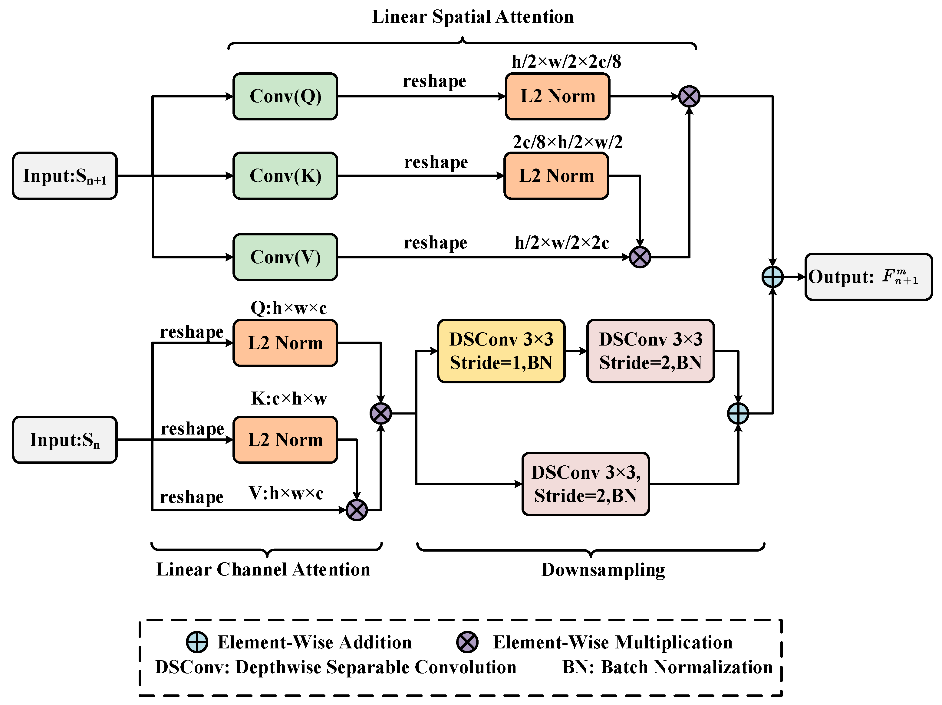
• An MSFR module is proposed to enhance and integrate adjacent global features. The MSFR module supplements the upper-layer features with details from the lower layer, reducing the loss of detailed information during global feature extraction.
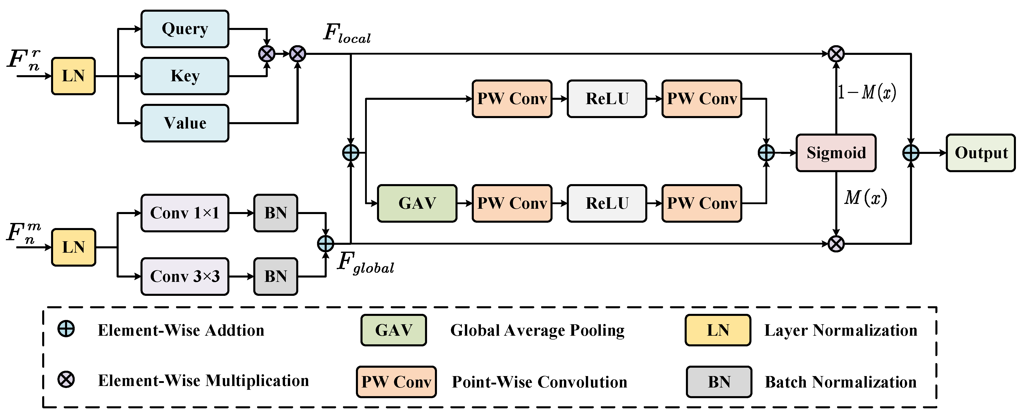
• An SBF module is introduced to facilitate efficient fusion of global and local features which performs adaptive fusion after narrowing the semantic differences between global and local features, resulting in more refined and comprehensive features.

The organization of the remaining sections is as follows. In Section 2, we briefly introduce the theoretical foundations related to Mamba and the applications of Mamba in the field of semantic segmentation tasks. In Section 3, we provide a comprehensive explanation of our proposed GLFFNet framework, including the design details of the MSFR and SBF modules. Section 4 validates the performance of the GLFFNet through experiments on three datasets. Finally, Section 5 provides a brief summary of our work.

2. Related Work

In this section, we primarily focus on the relevant applications of Mamba in image semantic segmentation tasks. To provide a comprehensive foundation for understanding the architecture of Mamba, we have included supplemental theoretical details of Mamba in Appendix A, which covers the basic principles of State Space Models (SSMs), their associated discretization and convolution computation methods, as well as the core concepts of Mamba.

Mamba in Semantic Segmentation Tasks

The core of Mamba is designed for processing 1-dimensional sequential data, whereas visual data are inherently non-sequential and contain spatial information. As a result, simple parallel selective scanning operations are not suitable for handling visual data. To adapt Mamba for visual tasks, Zhu et al. [34] proposed Vision Mamba. Vision Mamba first flattens a 2D image into 2D image patches, adds positional embeddings to preserve spatial information, and then uses bidirectional SSMs to process the image sequence. Due to the correlations between image patches, Vision Mamba adopts a sequential scanning approach that overlooks the issue of direction sensitivity. Another visual Mamba model VMamba [35] introduced an innovative 2D selective scan (SS2D) module. SS2D traverses along four scanning directions, which is beneficial for bridging the gap between the ordered nature of 1D selective scanning and the unordered structure of 2D visual data. This facilitates the collection of contextual information from various directions and perspectives. PlainMamba [36] used a zigzag scanning technique to maintain the spatial adjacency between tokens and prevent discontinuities. In order to explicitly integrate relative 2D positional information into the selective scanning process, PlainMamba also introduced a direction-aware update method. Huang et al. [37] highlighted that the effectiveness of SSMs in capturing image representations varies depending on the scanning direction. Therefore, they introduced a windowed selective scanning technique and a scanning direction search strategy, achieving significant improvements over existing models. The above methods have advanced the application of Mamba in visual tasks. Given that VMamba effectively captures the spatial structure and contextual information of visual data, we adopt VMamba [35] as an auxiliary encoder in our method.

The advantages of Mamba in extracting global information and performing efficient computations make it particularly well suited for image semantic segmentation tasks [38,39,40,41,42,43]. In the field of medical image segmentation, U-Mamba [44] represents an effective early attempt to apply Mamba to this domain. U-Mamba introduced a hybrid CNN-SSM module that combined the localized feature extraction strengths of convolutional layers with the long-range dependency modeling capabilities of SSMs. VM-UNet [45] serves as one of the most basic implementations of a pure SSM-based segmentation model. To unify the functionality of pre-trained models, Liu et al. [46] proposed Swin-UMamba for medical image segmentation. LightM-UNet [47] combines Mamba and UNet within a lightweight architecture, delivering exceptional segmentation performance. In the field of remote sensing image semantic segmentation, Samba [48] constructed Samba blocks based on Mamba blocks and employed them as encoders, effectively extracting multi-level semantic information. To address the limitation of Mamba, which is primarily designed for sequential data and lacks adaptability for 2D image data, RSMamba [49] introduced a dynamic multipath activation mechanism to enhance its capability for modeling non-sequential spatial information. RS3Mamba [32] is a novel dual-branch network designed for remote sensing image semantic segmentation. Hu et al. [50] introduced Pyramid Pooling Mamba (PPMamba), a network that combines CNN and Mamba for remote sensing semantic segmentation tasks. PPMamba performs selective scanning of feature maps from eight different directions, enabling it to capture a wide range of comprehensive feature information. Although the aforementioned works demonstrate the strong performance of Mamba in image semantic segmentation tasks, they often fail to adequately extract and utilize global and local information. Therefore, in order to further improve the segmentation performance of the model, it is urgent to propose a new method that can comprehensively and efficiently consider the global and local feature information.

3. Proposed Method

GLFFNet adopts a two-branch architecture, and the overall network structure is illustrated in Figure 1. GLFFNet consists of three parts: an auxiliary branch, main branch, and decoder. The auxiliary branch consists of a VMamba encoder and multi-scale feature refinement (MSFR) modules. The main branch adopts ResNet encoder and semantic bridging fusion (SBF) modules. The decoder consists of weight fusion (WF) modules and a final convolution module. The WF modules perform weighted feature fusion, while the final convolution module outputs the prediction results.

3.1. Global Feature Extraction and Enhancement

As shown in Figure 1, the auxiliary branch extracts global features using a VMamba encoder with linear computational complexity. Specifically, the VMamba encoder first uses the stem module to split the input image into multiple small patches, and then goes through four stages to create hierarchical feature representations. Each stage consists of downsampling layers and VSS blocks [35], where the downsampling layer is made via patch merging. When encoding, the input image $\mathrm{X}\in {\mathbb{R}}^{H\times W\times 3}$ is first decomposed into non-overlapping sub-blocks by the stem module, and then processed through four stages to generate hierarchical features $S_1\in {\mathbb{R}}^{C\times {\displaystyle \frac{H}{4}}\times {\displaystyle \frac{W}{4}}}$, $S_2\in {\mathbb{R}}^{2C\times {\displaystyle \frac{H}{8}}\times {\displaystyle \frac{W}{8}}}$, $S_3\in {\mathbb{R}}^{4C\times {\displaystyle \frac{H}{16}}\times {\displaystyle \frac{W}{16}}}$, and $S_4\in {\mathbb{R}}^{8C\times {\displaystyle \frac{H}{32}}\times {\displaystyle \frac{W}{32}}}$.

The four-layer features initially extracted by the VMamba encoder are often relatively rough. Compared with the lower-layer features, the semantic information of the upper-layer features is enhanced, but some details are lost. To reduce the loss of details during the hierarchical feature extraction, we design an MSFR module to specifically enhance and fuse the features of two adjacent layers, thereby achieving more refined global features. Specifically, to better aggregate feature information, we designed a downsampling module to adjust the feature sizes of adjacent layers. Then, based on the mechanism of linear attention [14], we developed a linear channel attention (LCA) module and a linear spatial attention (LSA) module to selectively enhance the features of the two adjacent layers. The structure of the MSFR module is shown in Figure 2. The MSFR module consists of an LCA module, LSA module, and downsampling module.

(1) Linear Spatial Attention: The LSA module is used to enhance the long-range spatial dependencies of the higher-level feature $S_{n+1}$, resulting in the feature $S_{n+1}^{\prime }$, which can be defined as follows:

$$\begin{array}{c}\hfill S_{n+1}^{\prime }={\displaystyle \frac{{\sum }_{n=1}^{N}V{\left(S_{n+1}\right)}_{c,n}+\left(\frac{Q\left(S_{n+1}\right)}{\parallel Q\left(S_{n+1}\right){\parallel }_2}\right)\left({\left(\frac{K\left(S_{n+1}\right)}{\parallel K\left(S_{n+1}\right){\parallel }_2}\right)}^{T}V\left(S_{n+1}\right)\right)}{N+\left(\frac{Q\left(S_{n+1}\right)}{\parallel Q\left(S_{n+1}\right){\parallel }_2}\right){\sum }_{n=1}^N{\left(\frac{K\left(S_{n+1}\right)}{\parallel K\left(S_{n+1}\right){\parallel }_2}\right)}_{c,n}^T}}\end{array}$$

(1)

where $Q\left(S_{n+1}\right)\in {\mathbb{R}}^{N\times D_k}$, $K\left(S_{n+1}\right)\in {\mathbb{R}}^{N\times D_k}$, $V\left(S_{n+1}\right)\in {\mathbb{R}}^{N\times D_v}$ represent the query matrix, key matrix, and value matrix generated by the convolution operation, N represents the number of pixels in the feature map, c represents the channel dimension, and n represents the flattened spatial dimension.

(2) Linear Channel Attention: Similarly, the LCA module is used to enhance the long-range channel dependencies of the lower-level feature $S_n$, resulting in the feature $S_n^{\prime }$, which can be defined as follows:

$$\begin{array}{c}\hfill S_n^{\prime }={\displaystyle \frac{{\sum }_{n=1}^{N}R{\left(S_n\right)}_{c,n}+\left(\frac{R\left(S_n\right)}{\parallel R\left(S_n\right){\parallel }_2}\right)\left({\left(\frac{R\left(S_n\right)}{\parallel R\left(S_n\right){\parallel }_2}\right)}^{T}R\left(S_n\right)\right)}{N+\left(\frac{R\left(S_n\right)}{\parallel R\left(S_n\right){\parallel }_2}\right){\sum }_{n=1}^N{\left(\frac{R\left(S_n\right)}{\parallel R\left(S_n\right){\parallel }_2}\right)}_{c,n}^T}}\end{array}$$

(2)

where $R(·)$ represents the reshape operation. Notably, both LCA and LSA modules have linear computational complexity. More details about the linear attention mechanism can be found in Reference [14].

(3) Downsampling: The purpose of the downsampling module is to adjust the shape of the enhanced features $S_n^{\prime }$ and $S_{n+1}^{\prime }$ to be consistent, which can be defined as follows:

$$\begin{array}{c}\hfill D\left({S_n}^{\prime }\right)=f_{\sigma }\left(f_{\delta }\left(S_n^{\prime }\right)+f_{\mu }\left(f_{\theta }\left(S_n^{\prime }\right)\right)\right)\end{array}$$

(3)

where D(·) represents the downsampling operation, $f_{\sigma }$ represents the ReLU activation function, $f_{\delta }$ and $f_{\mu }$ represent the $3\times 3$ depthwise separable convolution (DSConv) with a step size of 2, and $f_{\theta }$ represents the $3\times 3$ DSConv with a step size of 1. Each convolutional layer contains a batch normalization ($BN$) operation. Through the downsampling module processing, the shape of the enhanced feature $S_n^{\prime }$ is consistent with the enhanced feature $S_{n+1}^{\prime }$. Notably, compared to traditional convolutions, depthwise separable convolutions significantly reduce computational cost and model parameters with minimal impact on model performance.

Overall, the input features of the MSFR module are the adjacent layer features $S_n\in {\mathbb{R}}^{c\times h\times w}$ and $S_{n+1}\in {\mathbb{R}}^{2c\times {\displaystyle \frac{h}{2}}\times {\displaystyle \frac{w}{2}}}$ extracted by the VMamba encoder, where $n\in \{1,2,3\}$. The upper-layer feature $S_{n+1}$ is enhanced using the LSA module, which improves spatial dependency as described in Equation (1), yielding the feature $S_{n+1}^{\prime }$. Simultaneously, the feature $S_n$ is processed by the LCA module, enhancing channel dependency according to Equation (2), producing the output $S_n^{\prime }$. Afterward, the downsampling module processes the feature $S_n^{\prime }$, adjusting its shape to match $S_{n+1}^{\prime }$ as in Equation (3). Finally, the two enhanced features are added together to obtain the final enhanced feature $F_{n+1}^m$, as shown below:

$$\begin{array}{cc}\hfill F_{n+1}^m& \hfill =D\left(S_n^{\prime }\right)+S_{n+1}^{\prime }\hfill \end{array}$$

(4)

Through the above processing, the features of two adjacent layers are enhanced and aggregated through the MSFR module to obtain the global auxiliary features $F_1^m$, $F_2^m$, $F_3^m$ and $F_4^m$. The MSFR module leverages the LCA module to enhance the channel attention of lower-layer features, and the LSA module to enhance the spatial attention of high-level feature maps. Then, through cross-layer fusion, the lower-level features are used to supplement detailed information to the higher-level features. As a result, the MSFR module is capable of dynamically selecting and focusing on global features, reducing the loss of detailed information, and improving the network’s efficiency in leveraging these features.

3.2. Global–Local Feature Fusion

In order to fully leverage the advantages of both global and local features, we designed an SBF module that combines the strengths of window-based multi-head self-attention [20] and multi-scale channel attention [51]. The SBF module adaptively fuses features after reducing the semantic differences between global and local features, allowing for flexible and efficient feature integration. The structure of the SBF module is shown in Figure 3.

Given stage n, the VMamba global auxiliary feature is $F_n^m\in {\mathbb{R}}^{C_n^m\times h\times w}$, and the local feature extracted by ResNet is $F_n^r\in {\mathbb{R}}^{C_n^r\times h\times w}$, where $C_n^m$ and $C_n^r$ represent the number of channels for the two types of features, respectively. First, $F_n^r$ is processed through window-based multi-head self-attention [20] to enhance long-range dependency capabilities, resulting in the feature $F_{local}\in {\mathbb{R}}^{C_n^r\times h\times w}$. It is worth noting that this operation has linear complexity. Meanwhile, $F_n^m$ is processed through two parallel convolution branches to capture local detail information and adjust the number of channels to $C_n^r$, resulting in the feature $F_{global}\in {\mathbb{R}}^{C_n^r\times h\times w}$. The above process can be expressed by the following formula:

$$\begin{array}{cc}\hfill F_{local}& \hfill =W\left(F_n^r\right)\hfill \end{array}$$

(5)

$$\begin{array}{cc}\hfill F_{global}& \hfill ={Conv}_{1\times 1}\left(F_n^m\right)+{Conv}_{3\times 3}\left(F_n^m\right)\hfill \end{array}$$

(6)

where $W(·)$ is the window-based multi-head self-attention, ${Conv}_{1\times 1}(·)$ represents $1\times 1$ convolution with BN operation, and ${Conv}_{3\times 3}(·)$ represents $3\times 3$ convolution with BN operation. By integrating local information into global features and infusing global information into local features, the semantic differences between these features have been reduced.

To effectively fuse $F_{global}$ and $F_{local}$ at the same level, we first obtain a fused feature $F_{in}$ through simple addition of $F_{global}$ and $F_{local}$. Then, $F_{in}$ is processed through two parallel branches to obtain the local and global channel contexts, which are combined via broadcast addition to produce the fusion weight. The fusion weight is then used to perform adaptively weighted fusion on $F_{global}$ and $F_{local}$, resulting in the final fused feature. The calculation is described as follows:

$$\begin{array}{cc}\hfill {\mathrm{F}}_{in}& \hfill =F_{global}+{\mathrm{F}}_{local}\hfill \end{array}$$

(7)

$$\begin{array}{cc}\hfill \mathrm{L}\left({\mathrm{F}}_{in}\right)& \hfill =\mathcal{B}\left({\mathrm{PWConv}}_2\left(\delta \left(\mathcal{B}\left({\mathrm{PWConv}}_1\left({\mathrm{F}}_{in}\right)\right)\right)\right)\right)\hfill \end{array}$$

(8)

$$\begin{array}{cc}\hfill \mathrm{G}\left({\mathrm{F}}_{in}\right)& \hfill =\mathcal{B}\left({\mathrm{PWConv}}_2\left(\delta \left(\mathcal{B}\left({\mathrm{PWConv}}_1\left(\mathrm{g}\left({\mathrm{F}}_{in}\right)\right)\right)\right)\right)\right)\hfill \end{array}$$

(9)

$$\begin{array}{cc}\hfill \mathrm{M}\left({\mathrm{F}}_{in}\right)& \hfill =\sigma (\mathrm{L}\left({\mathrm{F}}_{in}\right)\oplus \mathrm{G}\left({\mathrm{F}}_{in}\right))\hfill \end{array}$$

(10)

$$\begin{array}{cc}\hfill {\mathrm{F}}_{output}& \hfill =\mathrm{M}\left({\mathrm{F}}_{in}\right)\otimes {\mathrm{F}}_{global}+\left(1-\mathrm{M}\left({\mathrm{F}}_{in}\right)\right)\otimes F_{local}\hfill \end{array}$$

(11)

where $L(·)$, $G(·)$ and $M(·)$ represent the operations for generating the local channel context, global channel context, and fusion weight, respectively. Specifically, $\mathcal{B}$ represents the batch normalization operation, $\sigma$ represents the sigmoid operation, $\delta$ represents the relu operation, and $\mathrm{PWConv}$ represents the point-wise convolution. The kernel size of ${\mathrm{PWConv}}_1$ is ${\displaystyle \frac{C_n^r}{t}}\times C_n^r\times 1\times 1$ and the kernel size of ${\mathrm{PWConv}}_2$ is $C_n^r\times {\displaystyle \frac{C_n^r}{t}}\times 1\times 1$, where t represents the channel reduction ratio. The symbol ⊕ represents broadcast addition, while the symbol ⊗ represents element-wise multiplication. Notably, $M\left(F_{in}\right)$ matches the dimensions of $F_{global}$ and $F_{local}$ and consists of real numbers between 0 and 1. $F_{output}\in R^{C_n^r\times h\times w}$ represents the final fused feature, which effectively combines the features from both encoders at the same stage, incorporating both global and local information.

By reducing semantic differences and controlling the fusion ratio of global and local features, we effectively mitigate noise and key information loss during the feature fusion process. At each stage of the main branch, the SBF module effectively fuses the global and local features of the same layer. The resulting fused features are then fed into the decoder via skip connections to obtain the prediction results.

4. Experiments

We conducted comparative and ablation experiments on the ISPRS Vaihingen, ISPRS Potsdam, and LoveDA datasets to validate the effectiveness of the proposed GLFFNet model. In this section, we first introduced the characteristics of these three public datasets. Next, we outlined the evaluation metrics and experimental setup used in our experiments. Following that, we performed comparative experiments, evaluating GLFFNet against several state-of-the-art semantic segmentation models on all three datasets. Then, we carried out an ablation study to assess the contribution of each module within GLFFNet to the overall performance. Finally, we analyzed the computational complexity of the model. It should be noted that the ISPRS datasets provide two types of ground truth: one with eroded boundaries and one without. In all our experiments, we used the version with eroded boundaries.

4.1. Dataset

Vaihingen: The ISPRS Vaihingen dataset consists of 33 remote sensing image tiles with an average size of $2000\times 2600$ pixels and a ground sampling distance (GSD) of 9 cm. Each image tile is composed of three spectral bands: near-infrared, red, and green. The dataset includes five foreground categories (impervious surfaces, buildings, low vegetation, trees, cars) and one background category (clutter). The clutter/background category includes other objects that are usually not of interest in semantic object classification in urban scenes. Among the 33 image tiles in the original Vaihingen dataset, we exploited ID 1, 3, 5, 7, 11, 13, 15, 17, 21, 23, 26, 28, 30, 32, 34, and 37 for training, ID 38 for validation, and the remaining 16 image tiles for testing [13]. In our experiments, all image tiles were cropped into multiple $1024\times 1024$ pixel patches to construct the training, validation, and test sets.

Potsdam: The ISPRS Potsdam dataset consists of 38 remote sensing images tiles with a GSD of 5 cm, each $6000\times 6000$ pixels. It involves the same category information as the Vaihingen dataset. The images are composed of four spectral bands: near-infrared, red, green, and blue. Note that we use only the red, green, and blue channels in our experiments. Excluding one erroneous image tile (ID: 7_10), we chose ID 2_13, 2_14, 3_13, 3_14, 4_13, 4_14, 4_15, 5_13, 5_14, 5_15, 6_13, 6_14, and 6_15 for testing, ID 7_13 for validation, and the remaining 23 image tiles for training [13]. Similar to the process for the Vaihingen dataset, all image tiles were cropped into multiple $1024\times 1024$ pixel patches to construct the training, validation, and test sets.

LoveDA: The LoveDA dataset [52] consists of 5987 high-resolution remote sensing images collected from three different cities, covering both urban and rural areas. It is well suited for semantic segmentation tasks due to its distinct characteristics, including multi-scale objects, complex background samples, and inconsistent class distributions. Each image has a GSD of 0.3 m and a size of $1024\times 1024$ pixels, with annotations covering seven categories: background, building, road, water, barren, forest, and agricultural. The original dataset is organized into three subsets, with 2522 images allocated to the training set, 1669 images designated for the validation set, and 1796 images reserved for the test set.

4.2. Experimental Setting

In the experiments, all models were implemented using the PyTorch (version 2.2.2) framework on a single NVIDIA GeForce RTX 2080 Ti GPU. The experiments were conducted on a computer equipped with a 12th Gen Intel Core i7-12700F CPU (2.10 GHz) and 32 GB of RAM. The AdamW optimizer was used with a base learning rate set to $1\times {10}^{-4}$, a weight decay set to $2\times {10}^{-4}$, and a batch size set to 4. The total epoch was set to 150. The learning rate was adjusted using a cosine annealing strategy. During training, images were randomly cropped to $512\times 512$ pixels, and data augmentation techniques such as random scaling (with scales of [0.5, 0.75, 1, 1.25, 1.5]), random vertical flipping, random horizontal flipping, and random rotation were applied. The loss function was set as the weighted average of the cross-entropy loss and the dice loss.

4.3. Evaluation Metrics

The performance of GLFFNet on the two datasets is evaluated by using the mean intersection over union (mIoU) and the F1 score, which are calculated based on the aggregated confusion matrix. The calculations are as follows:

$$\begin{array}{cc}\hfill \mathrm{P}& \hfill ={\displaystyle \frac{1}{N}}\sum _{k=1}^N{\displaystyle \frac{T{P}_k}{T{P}_k+F{P}_k}}\hfill \end{array}$$

(12)

$$\begin{array}{cc}\hfill \mathrm{R}& \hfill ={\displaystyle \frac{1}{N}}\sum _{k=1}^N{\displaystyle \frac{T{P}_k}{T{P}_k+F{N}_k}}\hfill \end{array}$$

(13)

$$\begin{array}{cc}\hfill \mathrm{F}1& \hfill =2\times {\displaystyle \frac{P\times R}{P+R}}\hfill \end{array}$$

(14)

$$\begin{array}{cc}\hfill \mathrm{mIoU}& \hfill ={\displaystyle \frac{1}{N}}\sum _{k=1}^N{\displaystyle \frac{T{P}_k}{T{P}_k+F{P}_k+F{N}_k}}\hfill \end{array}$$

(15)

where $T{P}_k$, $F{P}_k$, $T{N}_k$, and $F{N}_k$ indicate the true positive, false positive, true negative, and false negative for the specific object indexed as class k. P and R denote precision and recall, respectively.

4.4. Comparison Experiment

To validate the effectiveness of GLFFNet for semantic segmentation of HR²S images, we assessed the GLFFNet and benchmarked it against several leading supervised methods using the Vaihingen, Potsdam, and LoveDA datasets. The comparison methods can be divided into two categories. The first category includes networks that use a single model for both encoding and decoding, such as MANet [13], MAResU-Net [14], GCDNet [15], Swin-Unet [22], and VM-UNet [45]. Among them, MANet, MAResU-Net and GCDNet are CNN-based methods, Swin-Unet is a Transformer-based method, and VM-UNet is a Mambda-based method. The second category includes networks that use a hybrid model for encoding and decoding, such as UNetFormer [26], TransUNet [27] and RS3Mamba [32]. Among them, UNetFormer and TransUNet are methods based on CNN and Transformer, RS3Mamba is a method based on CNN and VMamba.

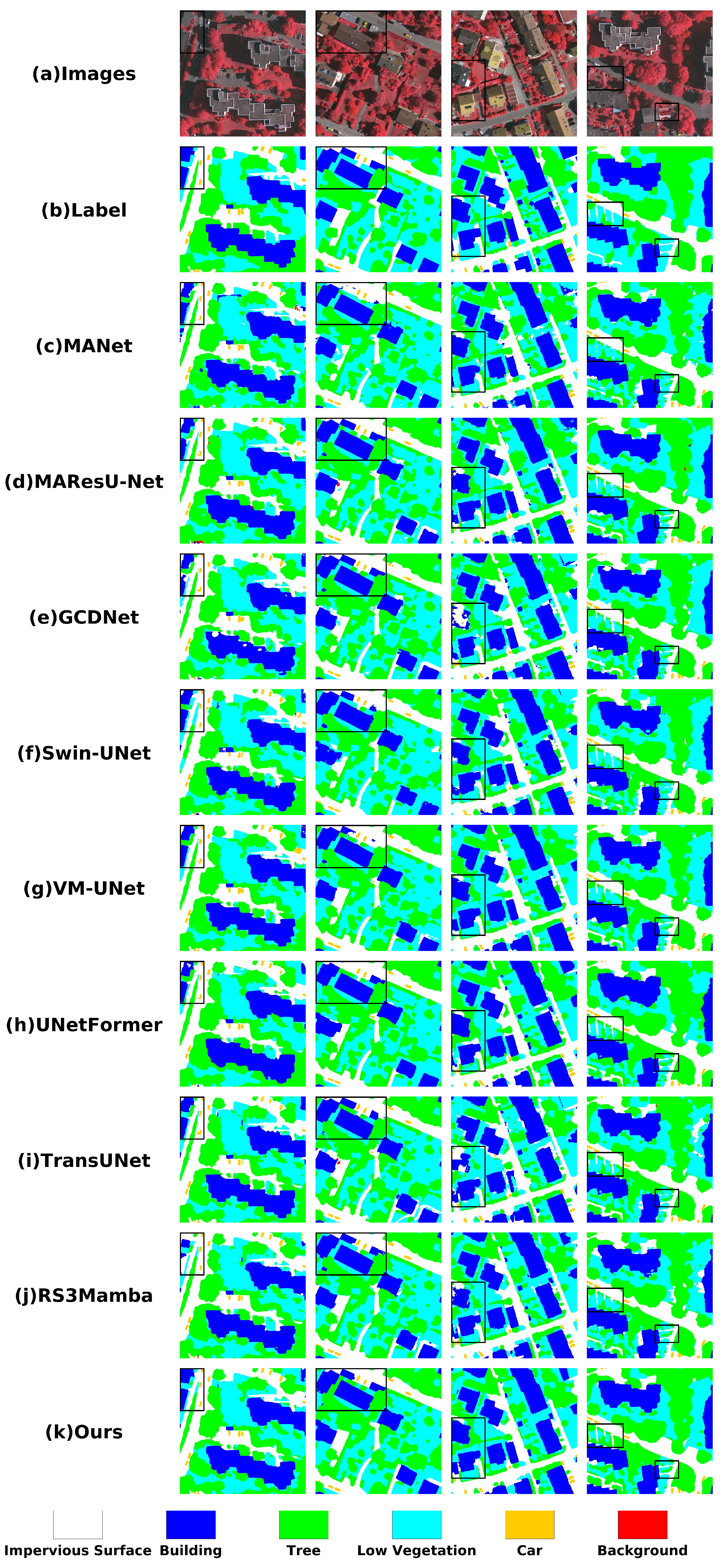
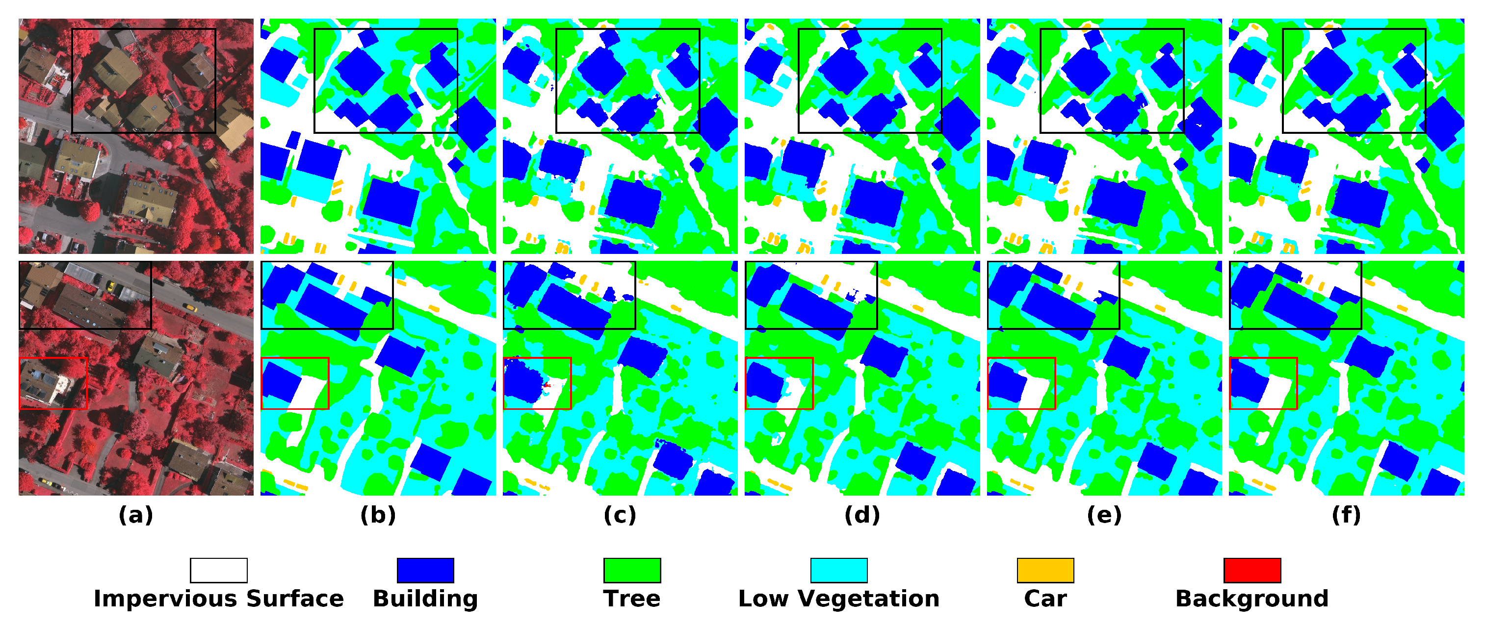
4.4.1. Results on Vaihingen

The comparative experimental results on the Vaihingen dataset are presented in

Table 1. Segmentation results of different models on the Vaihingen dataset. The accuracy of each category is presented in the format of F1/IoU (%).

Method	Imp. Surf.	Building	Low Veg.	Tree	Car	mF1 (%)	mIoU (%)
MANet [13]	96.28/92.82	94.39/89.37	83.38/71.50	89.72/81.36	86.67/76.48	90.09	82.31
MAResU-Net [14]	96.59/93.42	94.86/90.23	84.22/72.74	89.67/81.27	84.73/73.51	90.01	82.23
GCDNet [15]	95.98/92.27	93.79/88.32	83.25/71.30	89.44/80.90	86.41/76.08	89.77	81.77
Swin-Unet [22]	94.57/89.70	93.93/88.56	83.04/71.00	89.32/80.71	83.45/71.60	88.86	80.32
VM-UNet [45]	96.58/93.39	94.74/90.01	83.66/71.92	89.63/81.21	84.97/73.88	89.92	82.08
UNetFormer [26]	96.64/93.51	95.53/91.44	83.03/70.98	89.16/80.45	87.05/77.08	90.28	82.69
TransUNet [27]	95.39/91.18	95.66/91.68	84.71/73.47	90.00/81.81	87.19/77.29	90.59	83.09
RS3Mamba [32]	95.15/90.76	94.49/89.56	83.79/72.11	89.29/80.65	86.07/75.55	89.76	81.72
GLFFNet(Ours)	96.84/93.87	95.71/91.78	84.35/72.95	89.89/81.65	88.75/79.78	91.11	84.01

The values in bold represent the top-performing metrics in the table.

, where mF1 denotes the mean F1 score across all classes and values in bold represent the top-performing metrics in the table. The experimental outcomes indicate that the proposed GLFFNet achieves the highest mF1 (91.11%) and mIoU (84.01%). It outperforms networks based on a single model by at least 1.02% in mF1 and 1.70% in mIoU, underscoring the significance of global and local information in semantic segmentation. Compared to the hybrid models, GLFFNet improves the mF1 and mIoU scores by at least 0.52% and 0.92%, respectively, demonstrating superior overall performance due to the efficient utilization and comprehensive fusion of global and local feature information. Based on the results for each category, TransUNet [27] excels in the low vegetation and tree categories. However, due to the insufficient integration of global and local information, its performance in other categories and overall segmentation is inferior to that of GLFFNet. It is noteworthy that GLFFNet achieves the highest F1 score of 88.75% and an IoU score of 79.78% for the car category, indicating that it performs well in segmenting small objects.

The visualization results in Figure 4 illustrate the performance of GLFFNet on the Vaihingen dataset. The first three columns show that GLFFNet effectively delineates building boundaries with clarity and preserves complete structural shapes, while also distinguishing subtle differences between low vegetation and trees. In contrast, other methods (e.g., MANet [13], UNetFormer [26], and RS3Mamba [32]) display varying degrees of blurriness at the boundaries between buildings and other categories, resulting in less distinct class separations. In the fourth column, GLFFNet demonstrates a notable improvement in differentiating between impervious surfaces, low vegetation, and trees. Specifically, narrow impervious surface regions can be distinctly separated from the surrounding environment and exhibit clear edge contours. Conversely, other methods (e.g., MANet [13], GCDNet [15], and VM-UNet [45]) often misclassify these narrow regions, frequently interpreting them as low vegetation or trees. Overall, GLFFNet excels in capturing subtle inter-class differences in complex scenes, producing more coherent and accurate segmentation results.

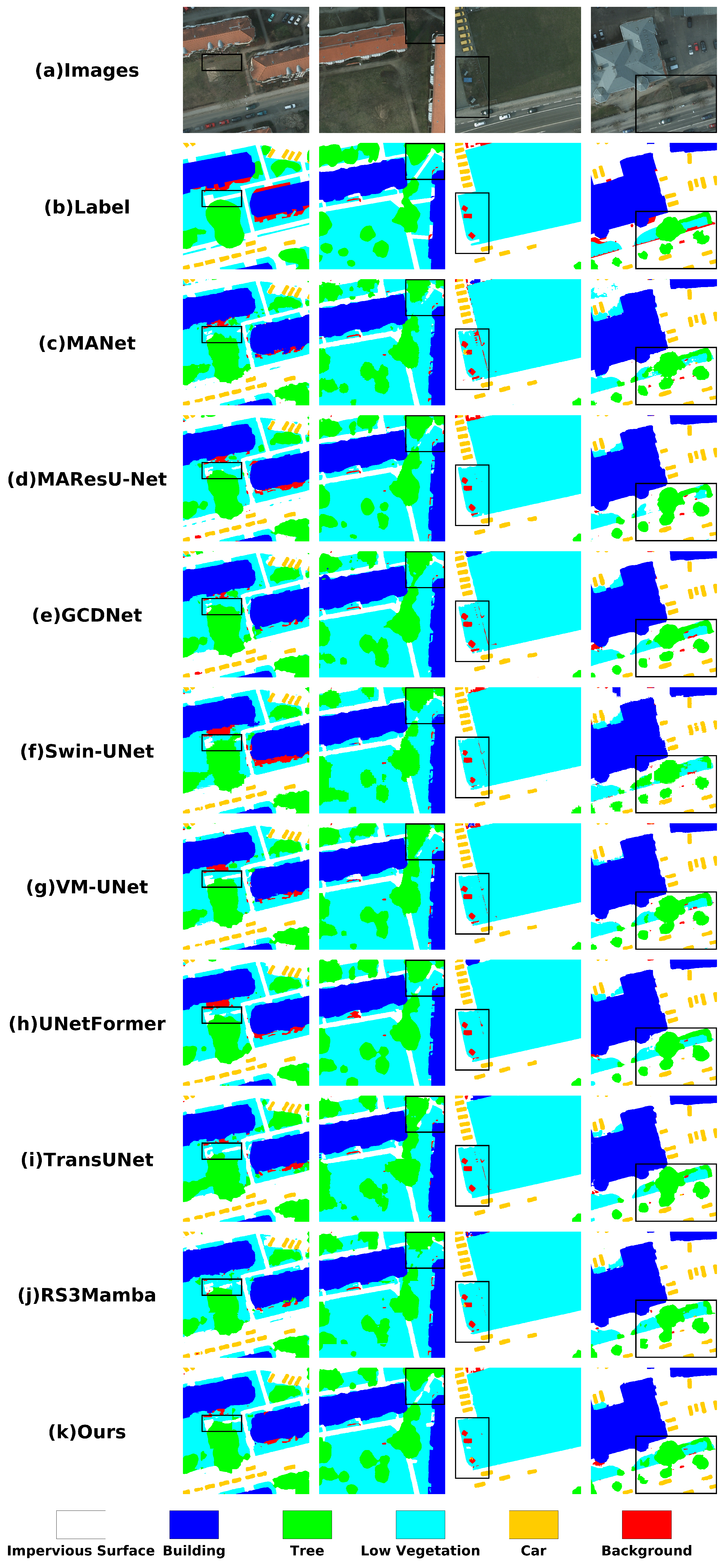
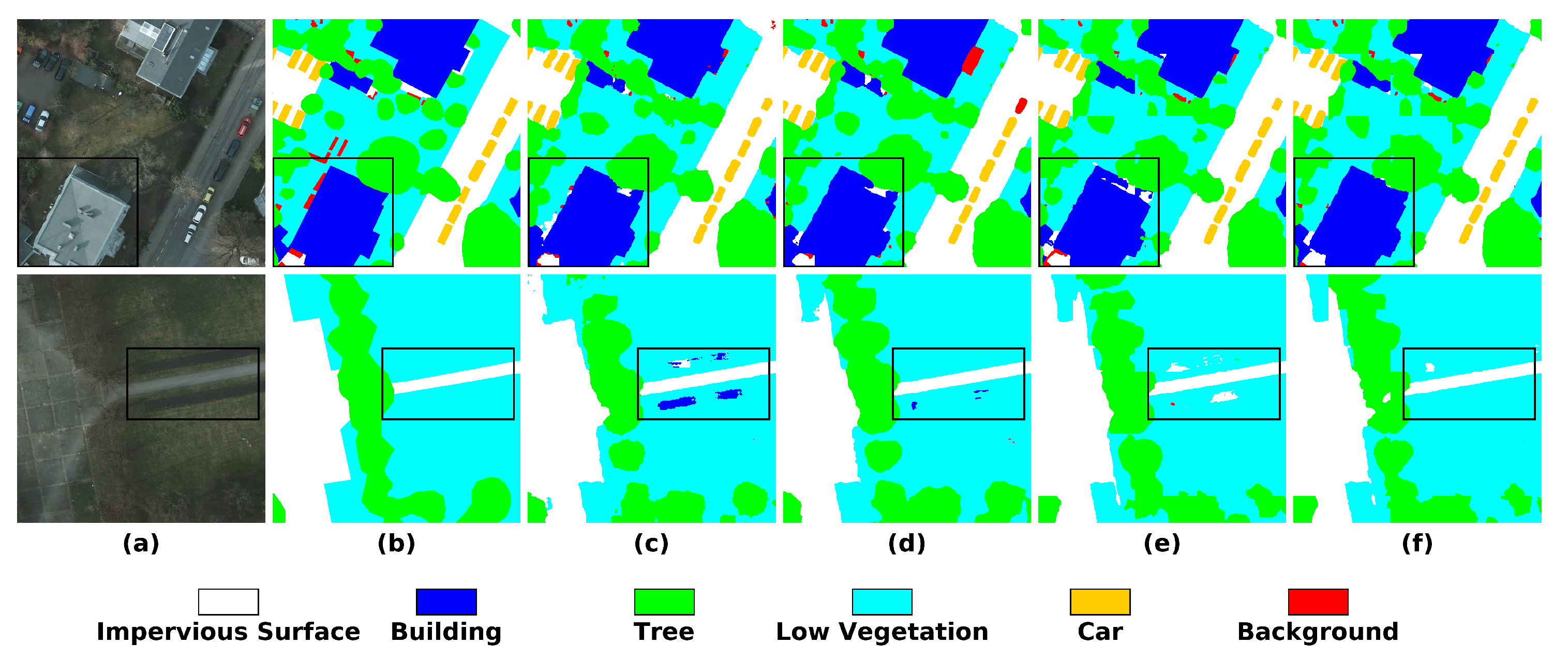
4.4.2. Results on Potsdam

Similarly, GLFFNet was evaluated on the Potsdam dataset alongside the current state-of-the-art segmentation models, with the comparative experimental results presented in

Table 2. Segmentation results of different models on the Potsdam dataset. The accuracy of each category is presented in the format of F1/IoU (%).

Method	Imp. Surf.	Building	Low Veg.	Tree	Car	mF1 (%)	mIoU (%)
MANet [13]	92.97/86.87	95.59/91.56	86.09/75.58	87.61/77.95	95.65/91.67	91.58	84.73
MAResU-Net [14]	93.19/87.26	96.20/92.69	86.47/76.16	87.88/78.38	95.68/91.73	91.88	85.24
GCDNet [15]	93.56/87.90	95.96/92.23	86.83/76.73	88.51/79.40	95.76/91.86	92.12	85.62
Swin-Unet [22]	93.00/86.93	95.52/91.42	86.11/75.61	87.63/77.98	94.30/89.21	91.31	84.23
VM-UNet [45]	93.77/88.28	96.21/92.70	86.70/76.53	87.42/77.65	95.27/90.97	91.88	85.23
UNetFormer [26]	93.77/88.28	96.48/93.20	86.61/76.38	88.09/78.72	95.81/91.96	92.15	85.71
TransUNet [27]	94.29/89.20	96.78/93.77	88.01/78.59	89.08/80.31	96.16/92.60	92.86	86.89
RS3Mamba [32]	93.83/88.38	96.83/93.86	87.61/77.96	88.39/79.20	95.56/91.50	92.45	86.18
GLFFNet(Ours)	94.47/89.52	97.30/94.75	88.46/79.32	89.53/81.05	96.39/93.04	93.23	87.54

The values in bold represent the top-performing metrics in the table.

. GLFFNet demonstrates strong overall performance, achieving an mF1 score of 93.23% and an mIoU score of 87.54%, surpassing most existing state-of-the-art methods. GCDNet [15] introduced a new dot-product attention mechanism to establish long-range dependencies across feature maps with varying receptive fields, effectively enhancing global feature representation. In comparison, GLFFNet leverages VMamba to directly extract global features and provide the main branch with enhanced global information. As a result, GLFFNet achieves a notable improvement over GCDNet [15], with mF1 increasing by 1.11% and mIoU by 1.92%. Furthermore, when compared to TransUNet [27], GLFFNet delivers additional improvements, with mF1 rising by 0.37% and mIoU by 0.65%. These performance gains can be attributed to GLFFNet’s effective integration of global and local feature information. Notably, GLFFNet exhibits strong performance across all categories when sufficient sample data are available, highlighting its robustness and adaptability.

The visualization results in Figure 5 demonstrate the performance of the GLFFNet on the Potsdam dataset. The results in the first and second columns demonstrate that GLFFNet can better distinguish impervious surfaces from low vegetation and trees. The third column reveals that GLFFNet achieves higher boundary precision and class differentiation in segmenting background regions within complex scenes. In contrast, other methods (e.g., MANet [13], GCDNet [15], and TransUNet [27]) exhibit noticeable misclassification in low-vegetation areas, where parts of the low vegetation are incorrectly identified as background regions. In the fourth column, GLFFNet excels in identifying cars, preserving their complete shapes and minimal interference from surrounding regions. Furthermore, GLFFNet effectively differentiates between low vegetation and trees, maintaining clear boundaries and a high degree of consistency between categories.

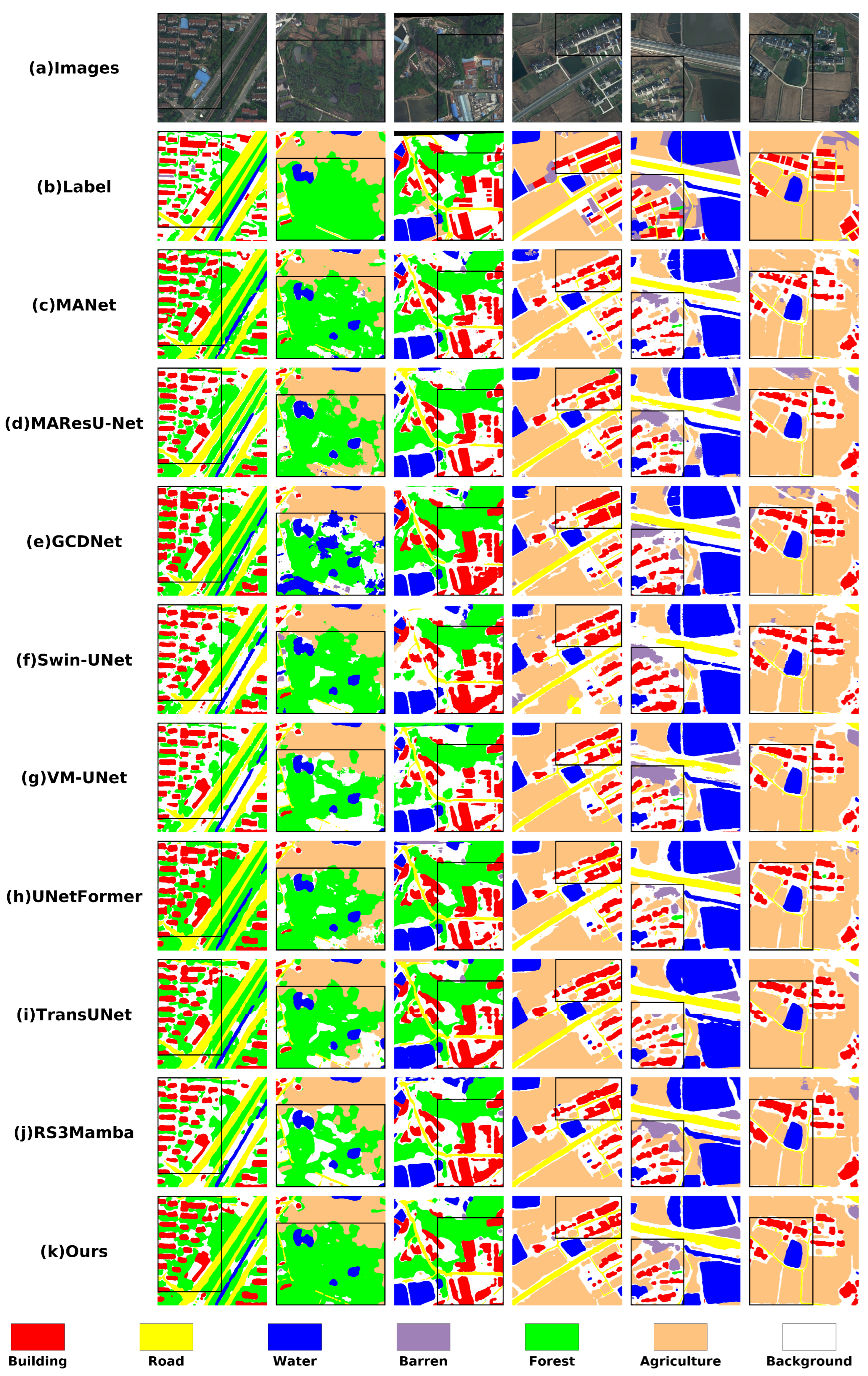
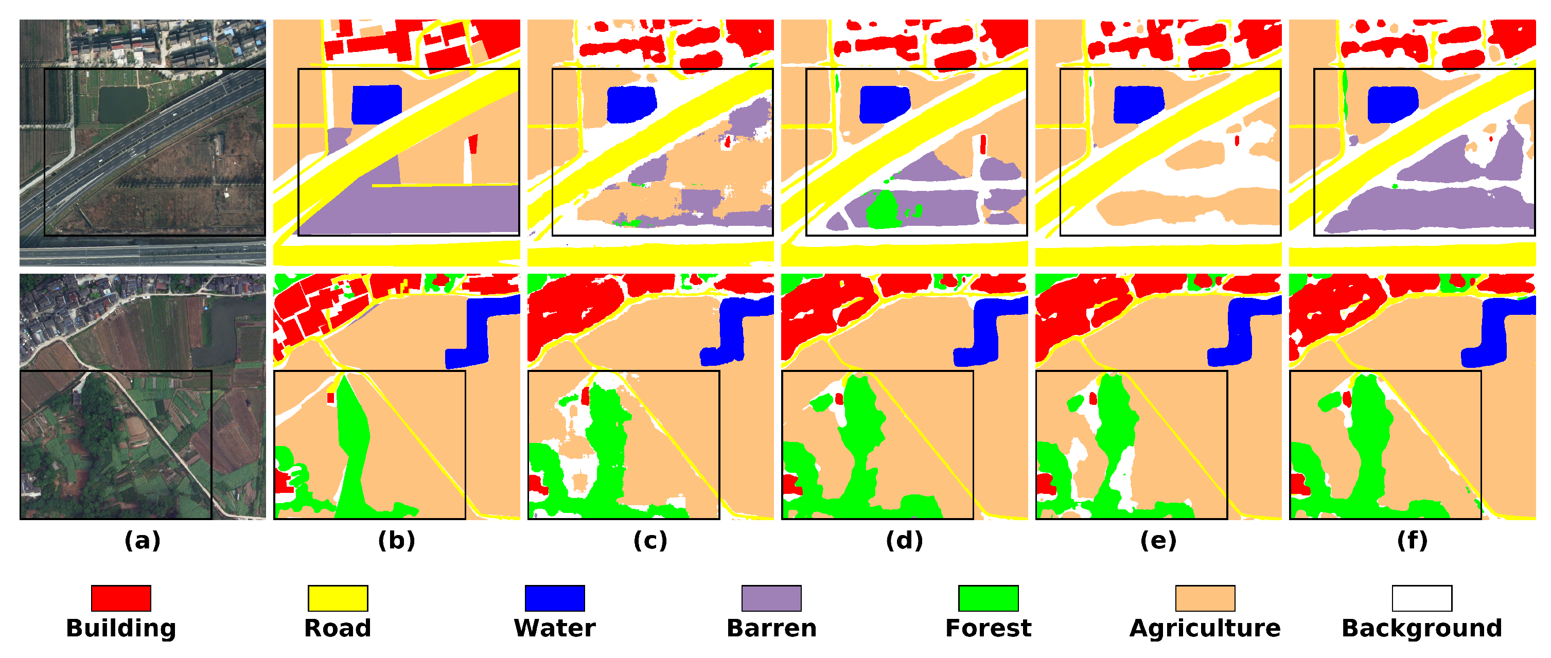
4.4.3. Results on LoveDA

The comparative experimental results on the LoveDA dataset are presented in

Table 3. Segmentation results of different models on the LoveDA dataset. The accuracy of each category is presented in the format of F1/IoU (%).

Method	Background	Building	Road	Water	Barren	Forest	Agricultural	mF1 (%)	mIoU (%)
MANet [13]	69.75/53.55	76.19/61.54	68.02/51.54	79.31/65.72	42.95/27.35	58.26/41.10	70.69/54.67	66.45	50.78
MAResU-Net [14]	69.83/53.65	76.65/62.15	70.29/54.19	77.76/63.62	49.72/33.09	59.85/42.71	71.01/55.05	67.87	52.06
GCDNet [15]	67.88/51.38	70.95/54.97	70.49/54.43	77.44/63.19	41.23/25.97	55.23/38.15	66.28/49.57	64.21	48.24
Swin-Unet [22]	68.92/52.58	72.70/57.11	67.32/50.73	80.46/67.31	47.52/31.16	60.13/42.99	65.81/49.04	66.12	50.13
VM-UNet [45]	69.42/53.17	75.63/60.82	69.69/53.49	80.68/67.62	50.75/34.00	53.92/36.91	66.87/50.23	66.71	50.89
UNetFormer [26]	66.75/50.09	76.17/61.51	71.43/55.56	80.77/67.75	46.69/30.46	59.74/42.59	67.77/51.25	67.05	51.32
TransUNet [27]	70.16/54.04	77.79/63.65	72.45/56.80	80.57/67.46	51.17/34.38	58.50/41.34	72.24/56.55	68.98	53.46
RS3Mamba [32]	70.42/54.35	78.86/65.10	71.94/56.18	82.54/70.27	50.30/33.60	57.03/39.89	75.16/60.20	69.46	54.23
GLFFNet(Ours)	68.27/51.83	79.01/65.31	71.28/55.37	80.41/67.24	53.14/36.19	60.33/43.19	78.03/63.98	70.07	54.73

The values in bold represent the top-performing metrics in the table.

. In terms of overall performance, GLFFNet achieves an mF1 score of 70.07% and an mIoU score of 54.73%, surpassing the majority of existing models. Compared to the single-encoder model VM-UNet [45] based on Mamba, GLFFNet achieves significant improvements, with an increase of 3.36% in mF1 and 3.84% in mIoU, while consistently delivering strong segmentation performance across all categories. These enhancements are attributed to GLFFNet’s dual-branch architecture, which effectively incorporates both global and local information. Compared to RS3Mamba [32], which also adopts a dual-branch structure, GLFFNet demonstrates stronger performance in the segmentation of buildings, barren, forests, and agricultural areas. However, the performance of GLFFNet is relatively weaker in the segmentation of road and water. This is likely due to the elongated and irregular shapes of these features, which challenge the network’s ability to effectively extract line-based and edge-specific characteristics. Overall, GLFFNet delivers better segmentation performance than most models, showcasing its advantages in general segmentation tasks.

The visualization results in Figure 6 showcase the performance of GLFFNet on the LoveDA dataset. The first three columns depict segmentation results in urban scenes, while the last three columns represent results in rural scenes. The black boxes in the first, third, and fourth columns highlight GLFFNet’s outstanding performance in segmenting the building category. Specifically, GLFFNet accurately identifies buildings and captures the shapes and boundaries of buildings with high precision. The second column emphasizes GLFFNet’s excellent performance in the forest category. In comparison to other methods (e.g., GCDNet [15], Swin-UNet [22], and VM-UNet [45]), which often produce redundant or irregular edges in forest segmentation, GLFFNet delivers more coherent results, effectively mitigating fragmentation and discontinuity. Similarly, the black boxes in the fifth and sixth columns underline GLFFNet’s superior segmentation performance in the agricultural category. In scenarios with complex agricultural distributions, MANet [13] and Swin-UNet [22] often misclassify parts of agricultural regions as background or other categories. Conversely, GLFFNet can accurately detect scattered agricultural regions, demonstrating its robustness and adaptability in diverse rural environments.

4.5. Ablation Study

To validate the effectiveness of GLFFNet, we conducted an ablation study on the Vaihingen, Potsdam, and LoveDA datasets to evaluate the contribution of each module to the overall performance. GLFFNet consists of four main modules: the main encode ResNet, the auxiliary encoder VMamba, the MSFR module, and the SBF module. In the ablation study, we analyzed and compared the impact of each module on the segmentation performance by gradually adding each module.

Table 4. Ablation study on the Vaihingen dataset. The accuracy of each category is presented in the format of IoU (%).

ResNet	VMamba	MSFR	SBF	Imp. Surf.	Building	Low Veg.	Tree	Car	mF1 (%)	mIoU (%)
✓				92.01	87.3	70.33	79.55	62.47	87.43	78.33
✓	✓			93.52	90.51	72.34	80.46	77.27	90.39 (↑2.96)	82.82 (↑4.49)
✓	✓	✓		93.66	90.85	73.25	81.37	78.86	90.88 (↑0.49)	83.60 (↑0.78)
✓	✓	✓	✓	93.87	91.78	72.95	81.65	79.78	91.11 (↑0.23)	84.01 (↑0.41)

The symbol ↑ indicates an improvement in evaluation metrics after adding a new module. The values in bold represent the top-performing metrics in the table.

and

Table 5. Ablation study on the Potsdam dataset. The accuracy of each category is presented in the format of IoU (%).

ResNet	VMamba	MSFR	SBF	Imp. Surf	Building	Low veg.	Tree	Car	mF1 (%)	mIoU (%)
✓				86.38	90.14	74.06	75.33	89.61	90.61	83.10
✓	✓			89.23	94.38	78.7	80.96	92.68	93.03 (↑2.42)	87.19 (↑4.09)
✓	✓	✓		89.27	94.48	79.08	80.96	93.11	93.14 (↑0.11)	87.38 (↑0.19)
✓	✓	✓	✓	89.52	94.75	79.32	81.05	93.04	93.23 (↑0.09)	87.54 (↑0.16)

The symbol ↑ indicates an improvement in evaluation metrics after adding a new module. The values in bold represent the top-performing metrics in the table.

present the results of the ablation study on the Vaihingen and Potsdam datasets, respectively.

Table 6. Ablation study on the LoveDA dataset. The accuracy of each category is presented in the format of IoU (%).

ResNet	VMamba	MSFR	SBF	Background	Building	Road	Water	Barren	Forest	Agricultural	mF1 (%)	mIoU (%)
✓				50.57	56.62	52.38	62.33	21.78	40.86	46.02	63.12	47.22
✓	✓			53.80	53.80	57.14	69.69	36.15	36.97	57.88	68.99 (↑5.87)	53.59 (↑6.37)
✓	✓	✓		55.50	64.38	51.99	69.97	34.17	40.45	62.18	69.38 (↑0.39)	54.09 (↑0.5)
✓	✓	✓	✓	51.83	65.31	55.37	67.24	36.19	43.19	63.98	70.07 (↑0.69)	54.73 (↑0.64)

The symbol ↑ indicates an improvement in evaluation metrics after adding a new module. The values in bold represent the top-performing metrics in the table.

shows the results on the LoveDA dataset. In these tables, the symbol ↑ indicates an improvement in evaluation metrics after adding a new module. It can be observed in Table 4, Table 5 and Table 6 that progressively adding various modules to the main branch ResNet results in improvements in both mF1 and mIoU metrics, demonstrating the effectiveness of each added module.

(1) Effectiveness of Global Information: After the VMamba is introduced to provide global information in the ResNet main branch, the segmentation performance for each category significantly improves. On the Vaihingen dataset, the mF1 score increases by 2.96% and the mIoU score by 4.49%. On the Potsdam dataset, the overall mF1 increases by 2.42% and the mIoU by 4.09%. On the LoveDA dataset, the overall mF1 increases by 5.87% and the mIoU by 6.37%. These results validate the importance of global information in segmentation tasks.

(2) Effectiveness of MSFR Module: After further introducing the MSFR module to refine and enhance global features at multiple scales, the segmentation performance of all categories improves to varying degrees. Notably, the performance improvement for the car category is the most significant in the Vaihingen and Potsdam datasets. This indicates that the inclusion of the MSFR module benefits segmentation tasks across various categories, with a particularly strong impact on the segmentation of small objects.

(3) Effectiveness of SBF Module: After further introducing the SBF module to the network, the overall performance on the Vaihingen dataset improves. Specifically, the segmentation accuracy for the impervious surfaces, buildings, trees, and cars categories shows effective improvement. On the Potsdam dataset, improvements are observed in the impervious surface, building, low vegetation, and tree categories, with an overall mF1 increase of 0.09% and an mIoU increase of 0.16%. On the LoveDA dataset, the inclusion of the SBF module leads to notable improvements across multiple categories, particularly in the building, barren, forest, and agricultural classes. The overall mF1 increases by 0.69%, reaching 70.07%, while the mIoU improves by 0.64%, reaching 54.73%. These results demonstrate the effectiveness of the SBF module.

Figure 7, Figure 8 and Figure 9 visually demonstrate the impact of each module on segmentation. As each module is progressively introduced, object contours become clearer and more complete, segmentation of small objects becomes more precise, and mutual interference between categories gradually decreases on the Vaihingen and Potsdam datasets. The ablation study results on the LoveDA dataset demonstrate that the introduction of each module significantly enhances the segmentation performance of the model. The VMamba module effectively mitigates boundary blurriness in categories such as buildings, roads, and forests, ensuring smoother transitions between different classes. The MSFR module strengthens multi-scale feature extraction, improving segmentation stability in complex scenes and reducing misclassification in small objects and boundary regions. The SBF module further refines the boundaries between forests and farmland, while also enhancing the shape and boundary details of barren land. Overall, these modules collectively improve the model’s class differentiation, boundary clarity, and detail preservation capabilities, resulting in more stable segmentation outcomes that closely align with the ground-truth labels.

4.6. Model Complexity Analysis

The model complexity of GLFFNet was evaluated using floating-point operation counts (FLOPs) and model parameters. FLOPs assess the computational complexity of the model, while parameters reflect its size. The training time of the model was represented by the average training time (ATT) per epoch, which was used to evaluate the model’s training efficiency. An optimal model would have lower FLOPs, fewer parameters, and shorter training time. It is worth noting that training time is influenced by various factors, such as model complexity, hardware resource utilization efficiency, optimization algorithms, and hyper-parameter settings.

Table 7. Model complexity analysis. All results are from the Vaihingen dataset.

Method	FLOPs (G)	Parameter (M)	ATT (s)	mF1 (%)	mIoU (%)
MANet	155.51	35.86	56.23	90.09	82.31
MAResU-Net	70.21	26.28	39.68	90.01	82.23
GCDNet	562.26	60.56	276.34	89.77	81.77
Swin-Unet	62.05	27.15	61.68	88.86	80.32
VM-Unet	32.96	22.04	132.19	89.92	82.08
UNetFormer	23.48	11.68	46.08	90.28	82.69
TransUNet	258.89	93.23	293.68	90.59	83.09
RS3Mamba	126.6	49.66	300.77	89.76	81.72
GLFFNet(ours)	154.46	64.22	283.79	91.11	84.01

The values in bold represent the top-performing metrics in the table.

shows the complexity analysis results for all the methods compared in this paper, where values in bold represent the top-performing metrics in the table. Notably, the FLOPs and parameter values for all methods were calculated based on two $512\times 512$ images using a single NVIDIA GeForce RTX 2080 Ti GPU. The results in Table 7 indicate that, compared to methods based on a single model, GLFFNet employs a parallel dual-branch structure, which increases the number of parameters, but achieves lower FLOPs than MANet and GCDNet. Compared to the lightweight model UNetFormer, although the FLOPs, parameter count, and training time are higher, the segmentation performance is significantly improved. Compared to RS3Mamba, GLFFNet introduces additional attention modules and feature fusion modules, leading to higher FLOPs and parameter counts. However, compared to TransUNet, which extracts features based on a Transformer architecture, GLFFNet significantly reduces the FLOPs and the number of parameters while still maintaining excellent segmentation performance. Overall, GLFFNet strikes a better balance between computational complexity and segmentation performance, highlighting its notable advantages.

5. Conclusions

In this paper, we propose a global–local feature fusion network (GLFFNet) for the semantic segmentation of HR²S images, mitigating the limitations of hybrid models in detailed information loss during feature extraction and insufficient fusion of global and local features. Specifically, GLFFNet adopts a dual-branch architecture, in which the auxiliary branch extracts global features through a VMamba encoder to provide global information for the main branch based on CNN. In addition, by introducing the MSFR module, we effectively reduce the loss of detailed information when extracting global features. This module performs cross-layer aggregation after enhancing the global features of two adjacent layers, resulting in a more comprehensive global feature representation that combines local details and global semantics. In order to avoid noise and loss of key information when fusing features, an SBF module is proposed. The SBF module performs adaptive fusion after narrowing the semantic differences between global and local features, achieving efficient fusion of global and local features. Comparative experiments and ablation studies on three public datasets fully demonstrate the effectiveness of GLFFNet. Although GLFFNet significantly improves the accuracy of semantic segmentation, it is still limited in segmenting certain objects with elongated and irregular shapes. Therefore, we will focus on addressing these limitations in future work. Additionally, we will continue to explore the potential of hybrid models for semantic segmentation tasks in HR²S images.

References

1. Wang, X.; Wang, H.; Jing, Y.; Yang, X.; Chu, J. A Bio-Inspired Visual Perception Transformer for Cross-Domain Semantic Segmentation of High-Resolution Remote Sensing Images. Remote Sens. 2024, 16, 1514. [Google Scholar] [CrossRef]
2. Alganci, U.; Soydas, M.; Sertel, E. Comparative research on deep learning approaches for airplane detection from very high-resolution satellite images. Remote Sens. 2020, 12, 458. [Google Scholar] [CrossRef]
3. Zhou, G.; Chen, W.; Gui, Q.; Li, X.; Wang, L. Split depth-wise separable graph-convolution network for road extraction in complex environments from high-resolution remote-sensing images. IEEE Trans. Geosci. Remote Sens. 2021, 60, 5614115. [Google Scholar] [CrossRef]
4. Li, Y.; Zhou, Y.; Zhang, Y.; Zhong, L.; Wang, J.; Chen, J. DKDFN: Domain knowledge-guided deep collaborative fusion network for multimodal unitemporal remote sensing land cover classification. ISPRS J. Photogramm. Remote Sens. 2022, 186, 170–189. [Google Scholar] [CrossRef]
5. Peng, D.; Bruzzone, L.; Zhang, Y.; Guan, H.; Ding, H.; Huang, X. SemiCDNet: A semisupervised convolutional neural network for change detection in high resolution remote-sensing images. IEEE Trans. Geosci. Remote Sens. 2020, 59, 5891–5906. [Google Scholar] [CrossRef]
6. Garcia-Garcia, A.; Orts-Escolano, S.; Oprea, S.; Villena-Martinez, V.; Garcia-Rodriguez, J. A review on deep learning techniques applied to semantic segmentation. arXiv 2017, arXiv:1704.06857. [Google Scholar]
7. Li, X.; Lei, L.; Kuang, G. Multilevel adaptive-scale context aggregating network for semantic segmentation in high-resolution remote sensing images. IEEE Geosci. Remote Sens. Lett. 2021, 19, 6003805. [Google Scholar] [CrossRef]
8. Tao, W.B.; Tian, J.W.; Liu, J. Image segmentation by three-level thresholding based on maximum fuzzy entropy and genetic algorithm. Pattern Recognit. Lett. 2003, 24, 3069–3078. [Google Scholar] [CrossRef]
9. Ronneberger, O.; Fischer, P.; Brox, T. U-net: Convolutional networks for biomedical image segmentation. In Proceedings of the Medical Image Computing and Computer-Assisted Intervention–MICCAI 2015: 18th International Conference, Munich, Germany, 5–9 October 2015; pp. 234–241. [Google Scholar]
10. He, K.; Zhang, X.; Ren, S.; Sun, J. Deep Residual Learning for Image Recognition. In Proceedings of the 2016 IEEE Conference on Computer Vision and Pattern Recognition (CVPR), Las Vegas, NV, USA, 27–30 June 2016; pp. 770–778. [Google Scholar] [CrossRef]
11. Wang, H.; Qiao, L.; Li, H.; Li, X.; Li, J.; Cao, T.; Zhang, C. Remote sensing image semantic segmentation method based on small target and edge feature enhancement. J. Appl. Remote Sens. 2023, 17, 044503. [Google Scholar] [CrossRef]
12. Su, Z.; Li, W.; Ma, Z.; Gao, R. An improved U-Net method for the semantic segmentation of remote sensing images. Appl. Intell. 2022, 52, 3276–3288. [Google Scholar] [CrossRef]
13. Li, R.; Zheng, S.; Zhang, C.; Duan, C.; Su, J.; Wang, L.; Atkinson, P.M. Multiattention Network for Semantic Segmentation of Fine-Resolution Remote Sensing Images. IEEE Trans. Geosci. Remote Sens. 2022, 60, 5607713. [Google Scholar] [CrossRef]
14. Li, R.; Zheng, S.; Duan, C.; Su, J.; Zhang, C. Multistage Attention ResU-Net for Semantic Segmentation of Fine-Resolution Remote Sensing Images. IEEE Geosci. Remote Sens. Lett. 2022, 19, 8009205. [Google Scholar] [CrossRef]
15. Cui, J.; Liu, J.; Wang, J.; Ni, Y. Global Context Dependencies Aware Network for Efficient Semantic Segmentation of Fine-Resolution Remoted Sensing Images. IEEE Geosci. Remote Sens. Lett. 2023, 20, 2505205. [Google Scholar] [CrossRef]
16. He, X.; Wang, Z.; Bai, L.; Fan, M.; Chen, Y.; Chen, L. Attention-Enhanced Urban Fugitive Dust Source Segmentation in High-Resolution Remote Sensing Images. Remote Sens. 2024, 16, 3772. [Google Scholar] [CrossRef]
17. Zhao, D.; Wang, C.; Gao, Y.; Shi, Z.; Xie, F. Semantic segmentation of remote sensing image based on regional self-attention mechanism. IEEE Geosci. Remote Sens. Lett. 2021, 19, 8010305. [Google Scholar] [CrossRef]
18. Song, W.; Zhou, X.; Zhang, S.; Wu, Y.; Zhang, P. GLF-Net: A Semantic Segmentation Model Fusing Global and Local Features for High-Resolution Remote Sensing Images. Remote Sens. 2023, 15, 4649. [Google Scholar] [CrossRef]
19. Vaswani, A.; Shazeer, N.; Parmar, N.; Uszkoreit, J.; Jones, L.; Gomez, A.N.; Kaiser, Ł.; Polosukhin, I. Attention is all you need. Adv. Neural Inf. Process. Syst. 2017, 30, 1–11. [Google Scholar]
20. Liu, Z.; Lin, Y.; Cao, Y.; Hu, H.; Wei, Y.; Zhang, Z.; Lin, S.; Guo, B. Swin Transformer: Hierarchical Vision Transformer using Shifted Windows. In Proceedings of the 2021 IEEE/CVF International Conference on Computer Vision (ICCV), Montreal, QC, Canada, 10–17 October 2021; pp. 9992–10002. [Google Scholar] [CrossRef]
21. Wang, L.; Li, R.; Duan, C.; Zhang, C.; Meng, X.; Fang, S. A Novel Transformer Based Semantic Segmentation Scheme for Fine-Resolution Remote Sensing Images. IEEE Geosci. Remote Sens. Lett. 2022, 19, 6506105. [Google Scholar] [CrossRef]
22. Cao, H.; Wang, Y.; Chen, J.; Jiang, D.; Zhang, X.; Tian, Q.; Wang, M. Swin-unet: Unet-like pure transformer for medical image segmentation. In Proceedings of the European Conference on Computer Vision, Tel Aviv, Israel, 23–27 October 2022; pp. 205–218. [Google Scholar]
23. Sun, Y.; Wang, M.; Huang, X.; Xin, C.; Sun, Y. Fast Semantic Segmentation of Ultra-High-Resolution Remote Sensing Images via Score Map and Fast Transformer-Based Fusion. Remote Sens. 2024, 16, 3248. [Google Scholar] [CrossRef]
24. Wang, H.; Li, X.; Huo, L.; Hu, C. Global and edge enhanced transformer for semantic segmentation of remote sensing. Appl. Intell. 2024, 54, 5658–5673. [Google Scholar] [CrossRef]
25. Song, W.; Nie, F.; Wang, C.; Jiang, Y.; Wu, Y. Unsupervised Multi-Scale Hybrid Feature Extraction Network for Semantic Segmentation of High-Resolution Remote Sensing Images. Remote Sens. 2024, 16, 3774. [Google Scholar] [CrossRef]
26. Wang, L.; Li, R.; Zhang, C.; Fang, S.; Duan, C.; Meng, X.; Atkinson, P.M. UNetFormer: A UNet-like transformer for efficient semantic segmentation of remote sensing urban scene imagery. ISPRS J. Photogramm. Remote Sens. 2022, 190, 196–214. [Google Scholar] [CrossRef]
27. Chen, J.; Lu, Y.; Yu, Q.; Luo, X.; Adeli, E.; Wang, Y.; Lu, L.; Yuille, A.L.; Zhou, Y. Transunet: Transformers make strong encoders for medical image segmentation. arXiv 2021, arXiv:2102.04306. [Google Scholar]
28. Wu, H.; Huang, P.; Zhang, M.; Tang, W. CTFNet: CNN-Transformer Fusion Network for Remote-Sensing Image Semantic Segmentation. IEEE Geosci. Remote Sens. Lett. 2024, 21, 5000305. [Google Scholar] [CrossRef]
29. Weng, L.; Pang, K.; Xia, M.; Lin, H.; Qian, M.; Zhu, C. Sgformer: A Local and Global Features Coupling Network for Semantic Segmentation of Land Cover. IEEE J. Sel. Top Appl. Earth Obs. Remote Sens. 2023, 16, 6812–6824. [Google Scholar] [CrossRef]
30. Wang, Z.; Xia, M.; Weng, L.; Hu, K.; Lin, H. Dual Encoder–Decoder Network for Land Cover Segmentation of Remote Sensing Image. IEEE J. Sel. Top Appl. Earth Obs. Remote Sens. 2024, 17, 2372–2385. [Google Scholar] [CrossRef]
31. Gu, A.; Dao, T. Mamba: Linear-time sequence modeling with selective state spaces. arXiv 2023, arXiv:2312.00752. [Google Scholar]
32. Ma, X.; Zhang, X.; Pun, M.O. RS3Mamba: Visual State Space Model for Remote Sensing Image Semantic Segmentation. IEEE Geosci. Remote Sens. Lett. 2024, 21, 6011405. [Google Scholar] [CrossRef]
33. Liu, M.; Dan, J.; Lu, Z.; Yu, Y.; Li, Y.; Li, X. CM-UNet: Hybrid CNN-Mamba UNet for Remote Sensing Image Semantic Segmentation. arXiv 2024, arXiv:2405.10530. [Google Scholar]
34. Zhu, L.; Liao, B.; Zhang, Q.; Wang, X.; Liu, W.; Wang, X. Vision mamba: Efficient visual representation learning with bidirectional state space model. arXiv 2024, arXiv:2401.09417. [Google Scholar]
35. Liu, Y.; Tian, Y.; Zhao, Y.; Yu, H.; Xie, L.; Wang, Y.; Ye, Q.; Liu, Y. Vmamba: Visual state space model. arXiv 2024, arXiv:2401.10166. [Google Scholar]
36. Yang, C.; Chen, Z.; Espinosa, M.; Ericsson, L.; Wang, Z.; Liu, J.; Crowley, E.J. Plainmamba: Improving non-hierarchical mamba in visual recognition. arXiv 2024, arXiv:2403.17695. [Google Scholar]
37. Huang, T.; Pei, X.; You, S.; Wang, F.; Qian, C.; Xu, C. Localmamba: Visual state space model with windowed selective scan. arXiv 2024, arXiv:2403.09338. [Google Scholar]
38. Zhang, Q.; Geng, G.; Zhou, P.; Liu, Q.; Wang, Y.; Kang, L. Link Aggregation for Skip Connection–Mamba: Remote Sensing Image Segmentation Network Based on Link Aggregation Mamba. Remote Sens. 2024, 16, 3622. [Google Scholar] [CrossRef]
39. Ding, H.; Xia, B.; Liu, W.; Zhang, Z.; Zhang, J.; Wang, X.; Xu, S. A novel mamba architecture with a semantic transformer for efficient real-time remote sensing semantic segmentation. Remote Sens. 2024, 16, 2620. [Google Scholar] [CrossRef]
40. Zhu, E.; Chen, Z.; Wang, D.; Shi, H.; Liu, X.; Wang, L. UNetMamba: An Efficient UNet-Like Mamba for Semantic Segmentation of High-Resolution Remote Sensing Images. IEEE Geosci. Remote Sens. Lett. 2025, 22, 6001205. [Google Scholar] [CrossRef]
41. Tsai, T.Y.; Lin, L.; Hu, S.; Chang, M.C.; Zhu, H.; Wang, X. UU-Mamba: Uncertainty-aware U-Mamba for Cardiac Image Segmentation. In Proceedings of the 2024 IEEE 7th International Conference on Multimedia Information Processing and Retrieval (MIPR), San Jose, CA, USA, 7–9 August 2024; pp. 267–273. [Google Scholar] [CrossRef]
42. Xu, Z.; Tang, F.; Chen, Z.; Zhou, Z.; Wu, W.; Yang, Y.; Liang, Y.; Jiang, J.; Cai, X.; Su, J. Polyp-mamba: Polyp segmentation with visual mamba. In Proceedings of the International Conference on Medical Image Computing and Computer-Assisted Intervention, Marrakesh, Morocco, 6–10 October 2024; pp. 510–521. [Google Scholar]
43. Wang, J.; Chen, J.; Chen, D.; Wu, J. LKM-UNet: Large Kernel Vision Mamba UNet for Medical Image Segmentation. In Proceedings of the International Conference on Medical Image Computing and Computer-Assisted Intervention, Marrakesh, Morocco, 6–10 October 2024; pp. 360–370. [Google Scholar]
44. Ma, J.; Li, F.; Wang, B. U-mamba: Enhancing long-range dependency for biomedical image segmentation. arXiv 2024, arXiv:2401.04722. [Google Scholar]
45. Ruan, J.; Xiang, S. Vm-unet: Vision mamba unet for medical image segmentation. arXiv 2024, arXiv:2402.02491. [Google Scholar]
46. Liu, J.; Yang, H.; Zhou, H.Y.; Xi, Y.; Yu, L.; Li, C.; Liang, Y.; Shi, G.; Yu, Y.; Zhang, S.; et al. Swin-umamba: Mamba-based unet with imagenet-based pretraining. In Proceedings of the International Conference on Medical Image Computing and Computer-Assisted Intervention, Marrakesh, Morocco, 6–10 October 2024; pp. 615–625. [Google Scholar]
47. Liao, W.; Zhu, Y.; Wang, X.; Pan, C.; Wang, Y.; Ma, L. Lightm-unet: Mamba assists in lightweight unet for medical image segmentation. arXiv 2024, arXiv:2403.05246. [Google Scholar]
48. Zhu, Q.; Cai, Y.; Fang, Y.; Yang, Y.; Chen, C.; Fan, L.; Nguyen, A. Samba: Semantic segmentation of remotely sensed images with state space model. Heliyon 2024, 10, e38495. [Google Scholar] [CrossRef]
49. Chen, K.; Chen, B.; Liu, C.; Li, W.; Zou, Z.; Shi, Z. RSMamba: Remote Sensing Image Classification With State Space Model. IEEE Geosci. Remote Sens. Lett. 2024, 21, 8002605. [Google Scholar] [CrossRef]
50. Hu, Y.; Ma, X.; Sui, J.; Pun, M.O. PPMamba: A Pyramid Pooling Local Auxiliary SSM-Based Model for Remote Sensing Image Semantic Segmentation. arXiv 2024, arXiv:2409.06309. [Google Scholar]
51. Dai, Y.; Gieseke, F.; Oehmcke, S.; Wu, Y.; Barnard, K. Attentional feature fusion. In Proceedings of the 2021 IEEE Winter Conference on Applications of Computer Vision (WACV), Waikoloa, HI, USA, 3–8 January 2021; pp. 3560–3569. [Google Scholar] [CrossRef]
52. Wang, J.; Zheng, Z.; Ma, A.; Lu, X.; Zhong, Y. LoveDA: A remote sensing land-cover dataset for domain adaptive semantic segmentation. arXiv 2021, arXiv:2110.08733. [Google Scholar]
53. Qu, H.; Ning, L.; An, R.; Fan, W.; Derr, T.; Liu, H.; Xu, X.; Li, Q. A survey of mamba. arXiv 2024, arXiv:2408.01129. [Google Scholar]
54. Pechlivanidou, G.; Karampetakis, N. Zero-order hold discretization of general state space systems with input delay. IMA J. Math. Control. Inf. 2022, 39, 708–730. [Google Scholar] [CrossRef]
55. Gu, A.; Dao, T.; Ermon, S.; Rudra, A.; Ré, C. Hippo: Recurrent memory with optimal polynomial projections. Adv. Neural Inf. Proces. Syst. 2020, 33, 1474–1487. [Google Scholar]
Figure 1. The overall architecture of GLFFNet.
Remotesensing 17 01019 g001
Figure 2. The detailed architecture of the MSFR module.
Remotesensing 17 01019 g002
Figure 3. The detailed architecture of the SBF module.
Remotesensing 17 01019 g003
Figure 4. Visualization results of different models on the Vaihingen dataset.
Remotesensing 17 01019 g004
Figure 5. Visualization results of different models on the Potsdam dataset.
Remotesensing 17 01019 g005
Figure 6. Visualization results of different models on the LoveDA dataset.
Remotesensing 17 01019 g006
Figure 7. Visualization results of the ablation study on the Vaihingen dataset. (a) Images. (b) Ground truth. (c) ResNet. (d) ResNet + VMamba. (e) ResNet + VMamba + MSFR. (f) ResNet + VMamba + MSFR + SBF.
Remotesensing 17 01019 g007
Figure 8. Visualization results of the ablation study on the Potsdam dataset. (a) Images. (b) Ground truth. (c) ResNet. (d) ResNet + VMamba. (e) ResNet + VMamba + MSFR. (f) ResNet + VMamba + MSFR + SBF.
Remotesensing 17 01019 g008
Figure 9. Visualization results of the ablation study on the LoveDA dataset. (a) Images. (b) Ground truth. (c) ResNet. (d) ResNet + VMamba. (e) ResNet + VMamba + MSFR. (f) ResNet + VMamba + MSFR + SBF.
Remotesensing 17 01019 g009