Abstract
To achieve high-precision positioning using the global navigation satellite system (GNSS), the onboard GNSS receiver integrates real-time kinematic (RTK) technology to enable centimeter-level positioning accuracy. Furthermore, array anti-interference technology is incorporated into the RTK receiver to enhance positioning reliability and mitigate interference in complex environments such as urban areas or regions with high electromagnetic activity. However, this approach can introduce signal distortion, which adversely affects the convergence of RTK positioning. To address the issue of bias introduced by interference suppression in RTK positioning, this paper focuses on error modeling and bias compensation through a phase bias compensation algorithm. A novel phase compensation algorithm is proposed, leveraging the anti-interference weighting coefficients of array elements and the anti-interference output signal. Compared to the conventional minimum variance distortionless response (MVDR) algorithm, the proposed method features a simpler architecture and achieves phase compensation at a lower computational cost using the power inverse (PI) algorithm. Simulation experiments demonstrate the effectiveness of the compensation method, achieving a mean phase bias of approximately 0.25 degrees and a variance of 4.62 degrees. This level of accuracy makes it highly suitable for UAVs operating in challenging environments where precision and reliability are paramount.
1. Introduction
Real-time kinematic (RTK) positioning technology has been developed to address both errors in the global navigation satellite system (GNSS) positioning process, such as those caused by ionospheric and tropospheric delays, as well as atomic clock synchronization issues [1,2]. This technology significantly enhances positioning accuracy by processing differential carrier phase observations between a reference station and a moving station in real time [3]. For unmanned aerial vehicles (UAVs), RTK positioning technology is particularly critical for applications requiring high precision, such as aerial mapping, precision agriculture, and autonomous navigation. However, the GNSS signals received by RTK systems are extremely weak, typically below −130 dBm, making them highly susceptible to interference [4]. This underscores the importance of robust anti-interference solutions to ensure reliable and precise positioning for UAV operations in challenging conditions.
In most cases, the noise power in GNSS signals is higher than the desired GNSS signal but lower than interference levels, posing a significant challenge for UAV operations that rely on precise positioning. Additionally, the direction of incoming satellite signals is often unknown to the GNSS receiver, further complicating the task of signal acquisition and interference mitigation [5]. Therefore, the primary challenge for GNSS receiver anti-interference technology lies in suppressing interference signals while ensuring that the gain of the useful GNSS signal is not compromised. To address this optimization problem, researchers have proposed the power inversion (PI) criterion. This criterion requires minimizing the output signal power after processing by an anti-interference algorithm, effectively filtering out interference while preserving the integrity of the useful GNSS signals [6]. Due to its straightforward implementation and proven effectiveness in interference suppression, the PI criterion has become the most widely adopted approach in UAV GNSS systems [7]. Other advanced criteria, such as the minimum mean square error (MMSE) criterion, maximum signal-to-interference plus noise ratio (MSINR) criterion, and minimum variance distortionless response (MVDR) criterion, have also been developed to enhance antenna anti-interference capabilities [8,9,10]. A comparative analysis of these anti-interference criteria is presented in Table 1, highlighting their respective advantages and suitability for UAV applications in challenging environments.

Table 1.
The comparison of different anti-interference criteria.
To address interference challenges in UAV operations, space array processing (SAP) and space-time array processing (STAP) have been developed based on established anti-interference criteria [11,12]. These techniques utilize antenna arrays to generate adaptive weights through anti-interference algorithms, which are applied to incoming signals to reduce interference power. However, the inherent characteristics of phased-array antennas and the weighting effects of adaptive anti-interference algorithms can compromise signal integrity, introducing measurement biases that are particularly critical for high-precision positioning systems like RTK systems. These biases arise from factors such as mutual coupling between array elements [13], amplitude and phase deviations among array units [14], inconsistencies in array RF channels [15], and phase biases directly or indirectly introduced by anti-interference algorithms [16]. Unlike common errors, these biases cannot be easily eliminated, posing significant challenges for UAV applications requiring centimeter-level accuracy, such as precision agriculture, aerial surveying, and autonomous navigation. Addressing these biases is essential to ensure reliable and precise RTK positioning in interference-prone environments.
To compensate for the deviations introduced by the anti-interference of array antennas, Kim U. S. adjusted the frequency characteristics of the signal by adding a finite impulse response (FIR) filter after each antenna element and suppressed measurement errors in the antenna array by trying to adjust the filter coefficients [17]. However, since the complexity of actual engineering implementation was not taken into account and real positioning performance tests needed to be conducted, the measurement bias system needed to be improved. Andrew O’Brien reduced the measurement bias introduced by the entire antenna array system by constraining the weights of the space-time array [18]. The simulation results indicate that this method has a good compensation effect on the carrier phase bias and meets the requirements of high-precision applications. However, the computational load is too large, and the cost in terms of engineering implementation remains too high. Jia Qiongqiong improved carrier phase estimation accuracy based on reference signal steering vector estimation combined with PI and MVDR algorithms [19]. The simulation experiments showed that a carrier phase bias of within 5 mm could be achieved. However, the hardware implementation was highly complex, significantly altered the existing receiver structure, and lacked real-time usability. Wang Yaoding proposed a distortion-less pseudo-code tracking space-time PI algorithm by keeping the coefficients of the temporal taps as real values and imposing constraints on the weights of the antenna array [20]. In addition, this algorithm was only applicable to pseudo-code ranging systems and was not applicable to carrier phase measurements. Li Song adopted a robust phase compensation technique to reduce the phase distortion. The proposed technique operates in real time and causes no processing delay while requiring only a minor modification to existing GNSS receivers [21]. Moreover, the method reduces the computational complexity. Nevertheless, the estimate uses an observation sequence with a window size of L, which will influence the estimation accuracy and the dynamic performance. In addition, the estimated phase bias is limited by the phase lock loop discriminator. If the phase bias is beyond the detection range of the discriminator, the phase bias cannot be accurately estimated [22]. Wu adopted blind adaptive beamforming based on direction lock loop. These algorithms can achieve similar effects to the MVDR algorithm by using the direction of arrival (DOA) estimation method without prior information. However, their complex hardware implementation restricts their application [23]. In conclusion, those methods require complex hardware implementation, which limits their application in low-cost general array receivers. The comparison of phase bias compensation algorithms is shown in Table 2.
Table 2.
The comparison of phase bias compensation algorithms.
The paper proposes an adaptive zeroing algorithm to compensate for the phase bias caused by the anti-interference algorithm of RTK. The algorithm consists of two steps. First, we present a rough bias compensation method based on array weighted-coefficient conjugation. Second, we propose fine bias compensation for the anti-interference output signal. The rough phase compensation is designed based on the PI algorithm, thus eliminating the need to obtain the satellite signal direction and reducing algorithm complexity compared to traditional phase bias compensation algorithms. The second step processes the anti-interference output signal, which has low hardware complexity. Therefore, the proposed algorithm does not require the direction of the incident signal and has low hardware complexity.
The structure of paper is as follows. In Section 2, the mathematical model of antenna array processing and RTK positioning are introduced. In Section 3, the characteristics of carrier phase bias are analyzed. Moreover, we introduce the algorithm. In Section 4, we simulate the anti-interference performance and discuss the phase bias compensation results.
2. Materials and Methods
This section begins by establishing the signal model for antenna array anti-interference algorithms. Following this, we analyze the impact of anti-interference effects on RTK positioning accuracy, a key consideration for UAV operations in environments prone to electromagnetic interference. In Section 2.4 and Section 2.5, we proposes the phase compensation method. First, we introduce the error analysis of the anti-interference algorithm in RTK positioning. Then, a bias compensation algorithm based on array weighted-coefficient conjugation for rough phase bias compensation. Finally, we propose a compensation algorithm based on the array anti-interference output signal for fine phase bias compensation.
2.1. Signal Model
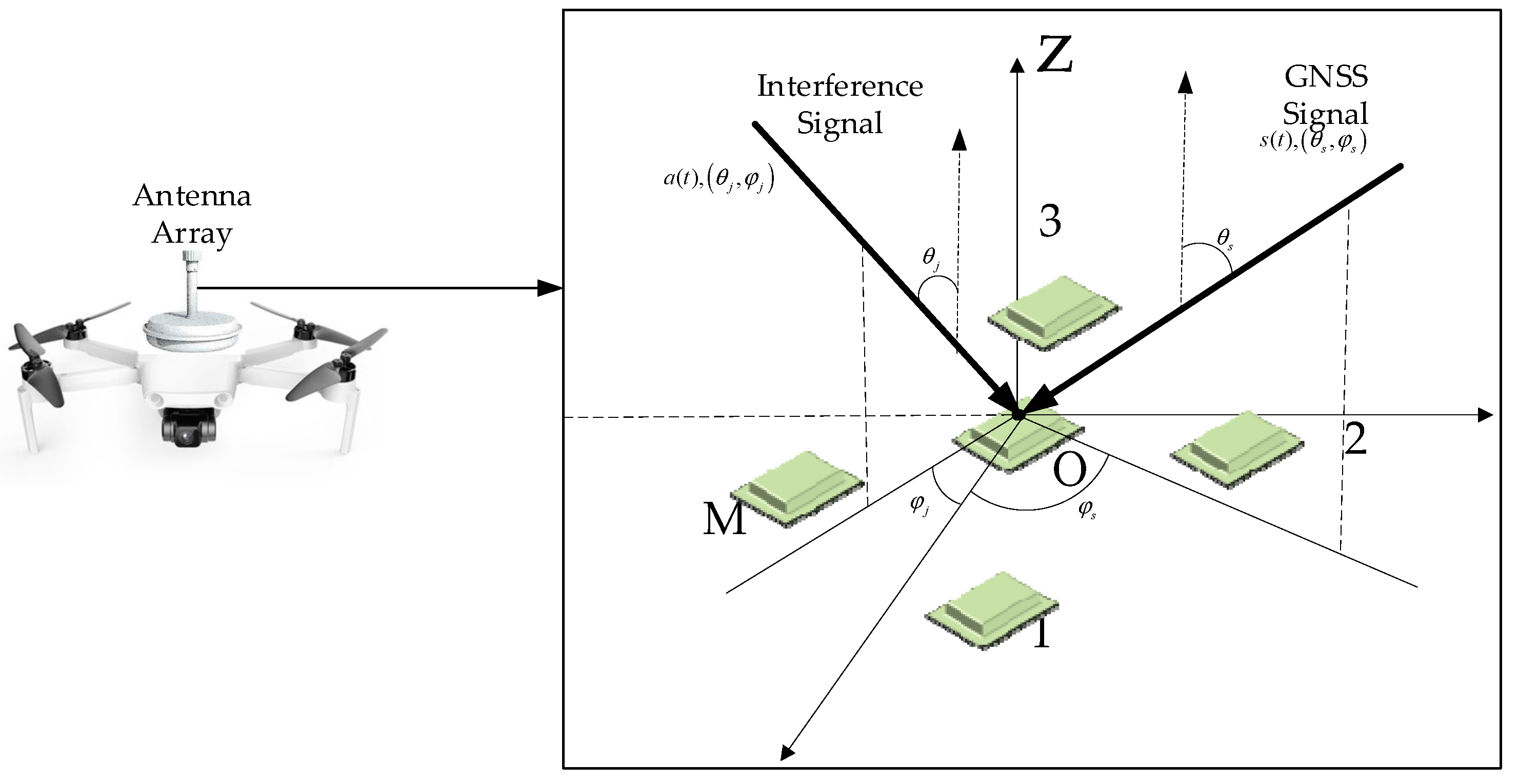
The antenna array is considered as comprising M ideal omnidirectional elements, ignoring the mutual coupling effects between elements [24,25]. Moreover, the antenna unit and radio frequency (RF) channel also meet the amplitude and phase consistency. Since the distance from the satellite signal to the ground is far greater than the array element spacing of the antenna array, it can be assumed that both the satellite signal and the interference signal are incident with plane waves. Therefore, the signal delay is only caused by the difference in the distance between the array elements.
Figure 1 is the antenna array structure. The 1, 2, 3, …, M is the antenna array number. And the incident signal with each antenna is shown in (1).
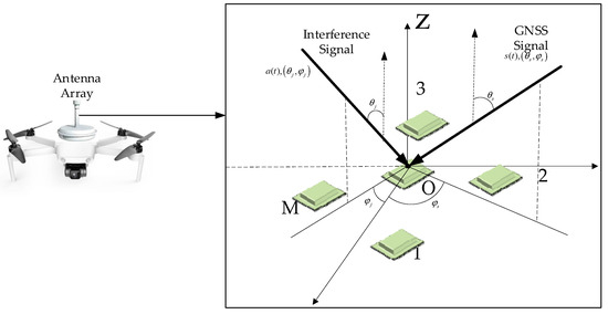
Figure 1.
The antenna array with incident signal.
Here, is the GNSS signal. . is the interference signal and is its number. is the noise that cannot be ignored.
The incident signal of the antenna array is as shown in (2).
Here, represents the steering vector of GNSS signal in each array element. represents the steering vector of the interference signal in each array element.
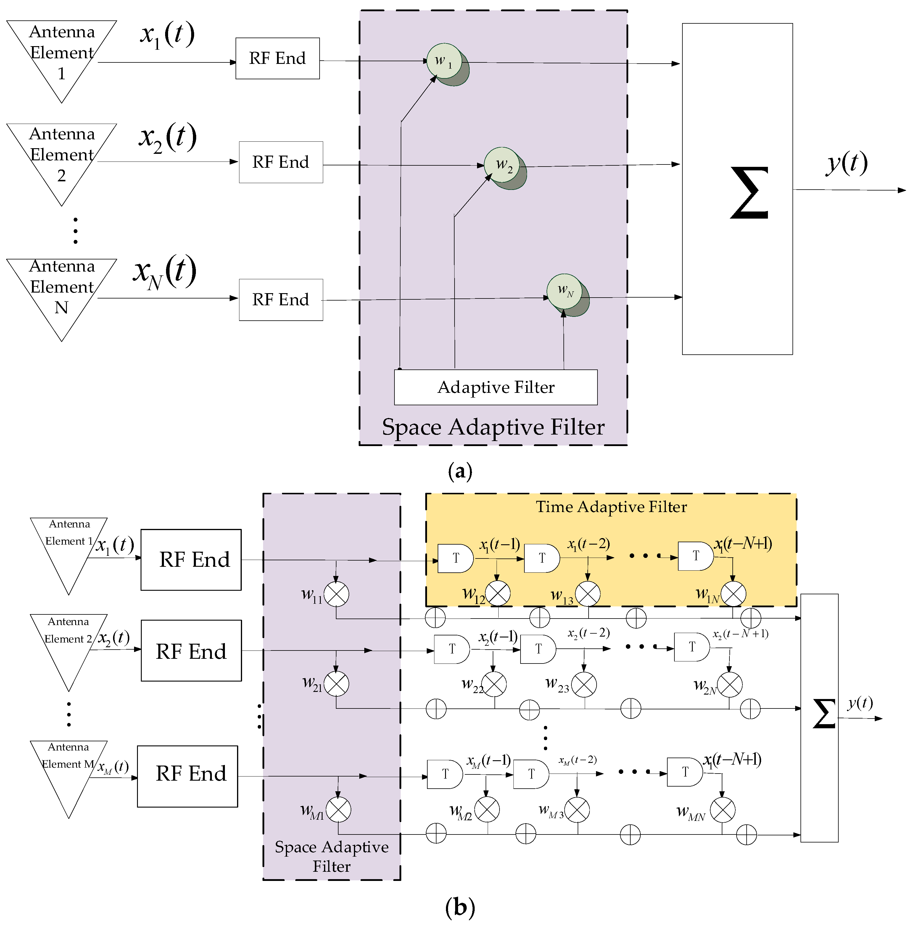
Figure 2a,b show the structures of SAP and STAP. The output signal of SAP is shown in (3).
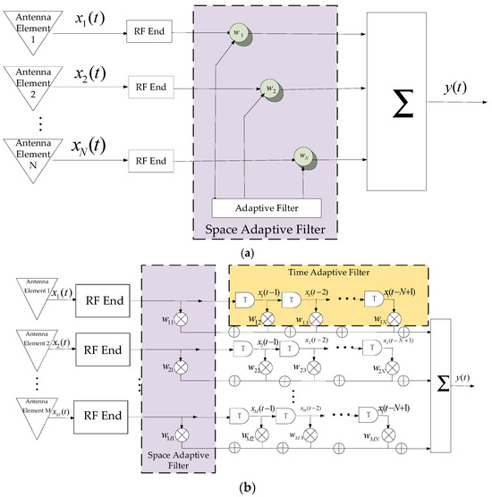
Figure 2.
The structure of SAP and STAP. (a) SAP; (b) STAP.
Here, is the antenna element weighting coefficient. is the array antenna receiving signal after RF front-end processing [26,27].
For STAP, the anti-interference weight coefficient consists of a time domain coefficient and space domain coefficient. The output signal of STAP is shown in (4).
Here, is the -dimensional space-time weighted vector. And is the -dimensional receiving signal vector [28].
2.2. Optimal Array Signal Weighting Criterion
In this section, we introduce the PI algorithm that does not need signal direction information and the MVDR algorithm that needs signal direction information.
The PI algorithm aims to minimize the output power of the array antenna and achieve the effect of filtering interference. The objective function and constraint function of the algorithm are as follows [29].
Here, is the antenna array output signal power. is the input signal autocorrelation matrix. is the antenna element weighting coefficient. is the unit vector, which ensures that the weight response of the first reference element signal is constant to ensure that the weight value solved is effective.
The optimal weight coefficient and antenna array output signal power are as follows.
The MVDR algorithm forms the beam on the desired signal based on the minimum output power. However, the algorithm should obtain the satellite signal arrival information. The objective function and constraint function of the algorithm are as follows [30].
Here, is the expected signal direction vector.
The optimal weight coefficient and antenna array output signal power are as follows.
2.3. Influence of Anti-Interference Algorithm on RTK Positioning
In RTK positioning, the motion station and the reference station receive two satellites signal at the same epoch. The receiver of the motion station makes a double difference in stations and satellites to eliminate clock difference, ionospheric delay, and tropospheric delay. And the double-difference carrier phase result is shown in (9).
Here, is the wavelength of the carrier. represents the double-difference geometric distance. represents the double-difference integer ambiguity. denotes the double-difference observation noise. And the unknown parameters in (9) are .
Then, the Kalman filter is adopted to estimate the . Its state equation and observation equation can be expressed as follows.
Here, k is the observation epoch time. is the state vector at k. Assuming the satellite number is 4, the . is the motion station location. is the double-difference integer ambiguity of satellites. is the state transition matrix. is the control-input model that is applied to the process noise . is the observation result at k. is the observation model, which maps the true state space into the observed space. is the observation noise, which is assumed to be zero-mean Gaussian white noise [31,32].
However, the phase bias introduced by the anti-interference algorithm itself will directly affect the carrier phase observations, thereby influencing the positioning distance. Therefore, the carrier phase observation is shown in (11).
In (11), is the phase bias that is introduced by the anti-interference algorithm.
According to the prediction and update process of the Kalman filter, the bias introduced in the carrier phase observation affects the observation matrix ; then, at the time of epoch k, the variable of state estimation can be shown as
And the predicted value of state at epoch k + 1 is , where . Therefore, the state estimation at k + 1 is as shown in (13):
The state estimation error at the time of k + 1 epoch is as shown in (14):
The observation matrix error of epoch k leads to the state estimation error of epoch k, and this error continues to be transmitted in the next epoch. And the impact on RTK positioning cannot be ignored, which will lead to a large RTK positioning bias or failure to obtain a position result. It is necessary to compensate for the bias introduced by the anti-interference algorithm to achieve the positioning of the RTK system.
2.4. Error Analysis
Assume the receiving signal of antenna element k is as shown in (15).
The satellite signal is . is the steering vector of the satellite signal in antenna element k. The interference signal is . is the steering vector of the interference signal in antenna element k. The noise is .
The antenna array steering vector is shown in (16):
The coordinate of antenna element k is . The unit vector of the incident signal direction is . N is the element number of the antenna array. Therefore, the output signal of the antenna array is as shown in (17).
Here, , and .
For the SAP PI algorithm, the optimal weight coefficient is a complex value that is only constrained by . Therefore, based on (3) and (17), the output of the antenna array signal is
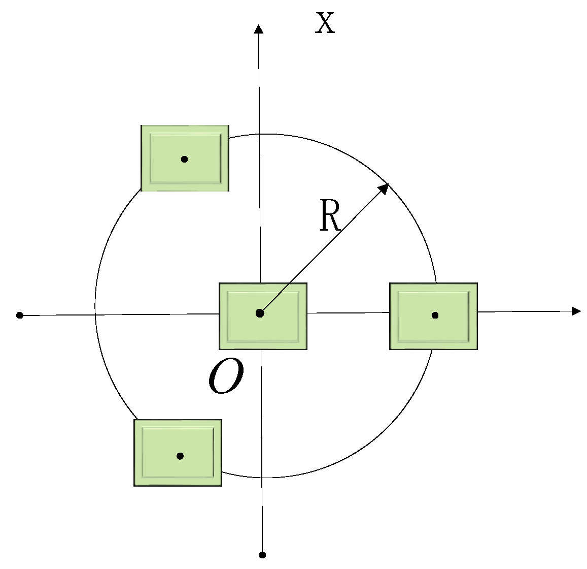
Therefore, the phase bias of SAP PI algorithm is . Taking the four-element array as an example, the array distribution is shown in Figure 3.

Figure 3.
The four-element array.
Assume that the reference element is at the origin point, the rest of the elements are evenly distributed on the circle, and the coordinates of the four elements are . And the phase bias of SAP algorithm is as shown in (19).
Figure 4 shows the distribution of the phase bias.
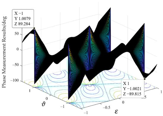
Figure 4.
The phase bias distribution of four-element antenna array.
For the STAP PI algorithm, the optimal weight coefficient is also a complex number, but the dimension adds the time domain parts compared with SAP. Therefore, the steering vector becomes the Kronecker product of the spatial domain steering vector and the time domain tap vector, which is the expansion of the dimension in the spatial domain, but also a complex number.
For the SAP MVDR algorithm and STAP MVDR algorithm, the optimal weight coefficient is a complex value constrained by . Therefore, the algorithms do not introduce phase bias.
2.5. The Bias Compensation Method for Anti-Interference Algorithm
In this section, we take a simple array element distribution as an example and provide the sufficient conditions for error compensation. First, we provide the rough bias compensation method based on array weighted-coefficient conjugation. Second, we propose the bias compensation at an anti-interference output signal.
2.5.1. Bias Compensation Method Based on Array Weighted-Coefficient Conjugation
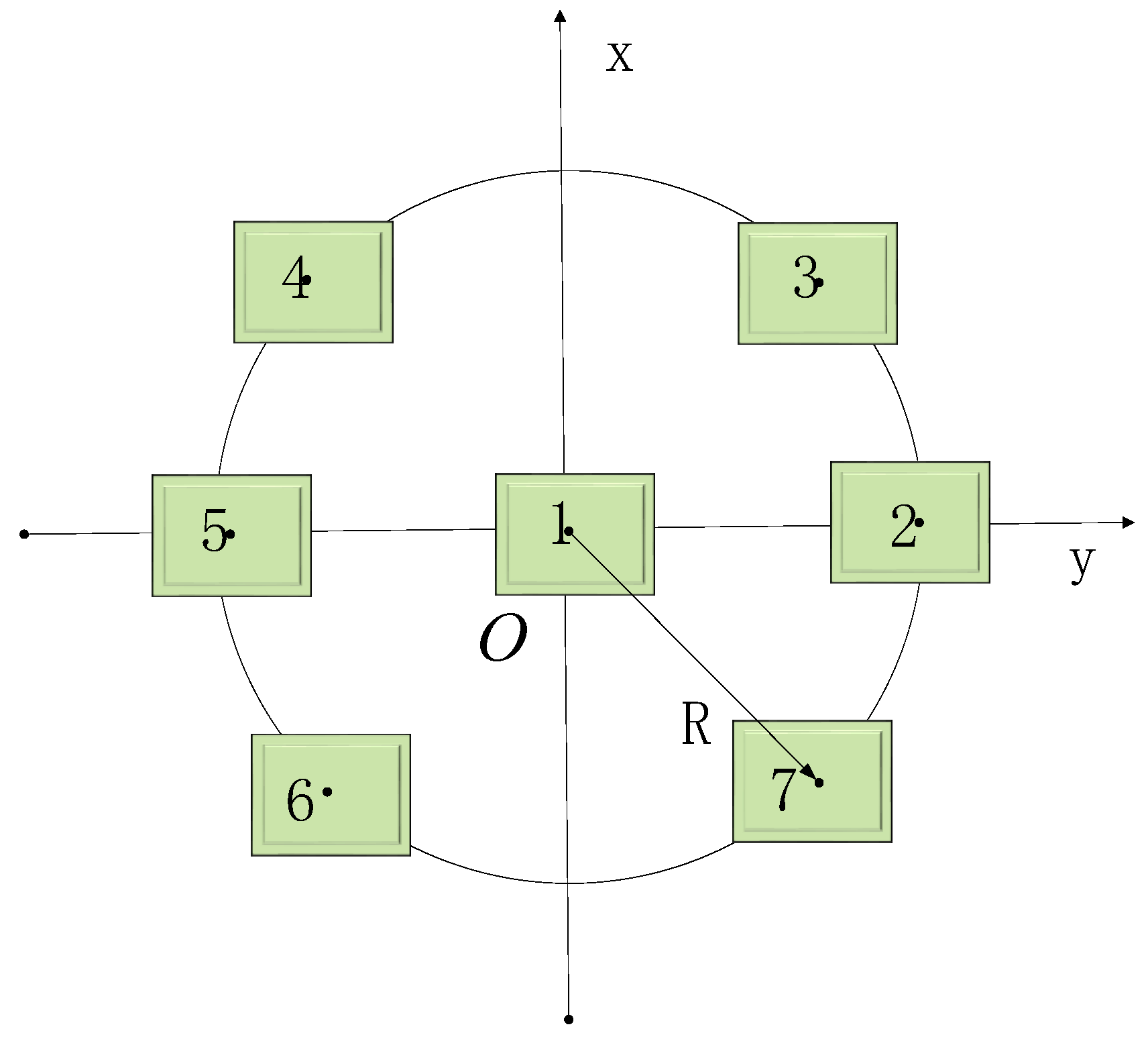
We take seven elements as an example to illustrate the bias compensation algorithm with an odd number of elements. The distribution of elements is as shown in Figure 5.
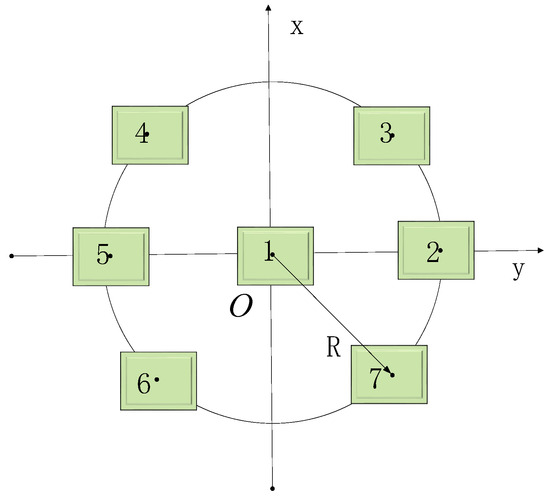
Figure 5.
The distribution of seven elements.
In the antenna array, elements 2 and 5 are symmetrical, elements 3 and 6 are symmetrical, elements 4 and 7 are symmetrical, and the coordinates are , , , , , , and . Therefore, the antenna element delay and weight coefficients have the following relationship.
The phase bias of the PI algorithm in the antenna array is shown in (21).
Therefore, the weight coefficient of the seven-element antenna array is a real value that does not introduce phase bias. Based on the analysis, we propose the seven-element zero-phase-bias PI criterion in SAP as shown in (22).
The terms in (22) can be expressed as (23) with a matrix.
Here, , and . And (23) can be simplified as (24).
The Lagrange derivation is used to obtain the optimal solution, and the Lagrange expression is shown in (25).
Here, is an unknown constant vector and partial derivative with respect to . The result is (26).
And (26) can be expressed as (27).
Substituting (27) into (23), we can obtain (28).
Combining (28), we obtain (29).
Simplifying (29), we obtain (30).
Substituting into (28) and (29), we can obtain (31).
Here, is the weight coefficient.
2.5.2. Bias Compensation at Anti-Interference Output Signal
To improve the phase bias compensation accuracy, we adopt phase bias compensation after the anti-interference algorithm to achieve bias compensation. The steps are as follows.
Step 1. Obtaining the signal after the SAP algorithm based on (31);
Step 2. Multiplying the reciprocal of as in (32).
is the output signal after the SAP algorithm.
Obviously, it is feasible in theory, and the method is simple. The structure is shown in Figure 6. At the receiver end, each channel eliminates the bias for the specific direction signal.
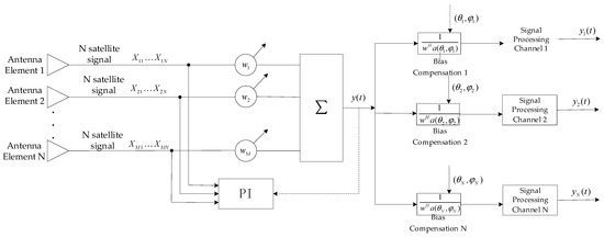
Figure 6.
The structure of phase bias compensation algorithm based on antenna array output signal.
3. Results
3.1. The Phase Bias Simulation
Assume the incident signal from . The RF is 1268.52 MHz, intermediate frequency (IF) is 46.52 MHz, and sampling frequency is 62 MHz. A broadband interference signal is taken from the nearby angular domain , . The phase biases that has introduced by the SAP PI algorithm, STAP PI algorithm, and SAP MVDR algorithm are as follows.
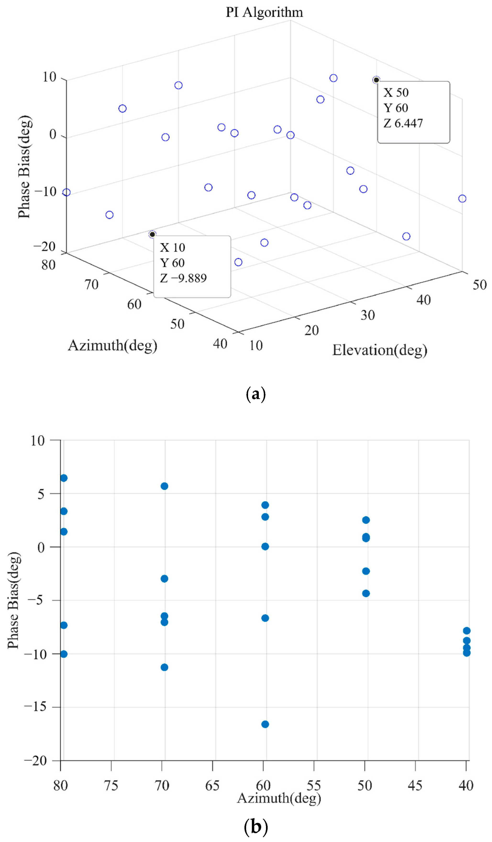
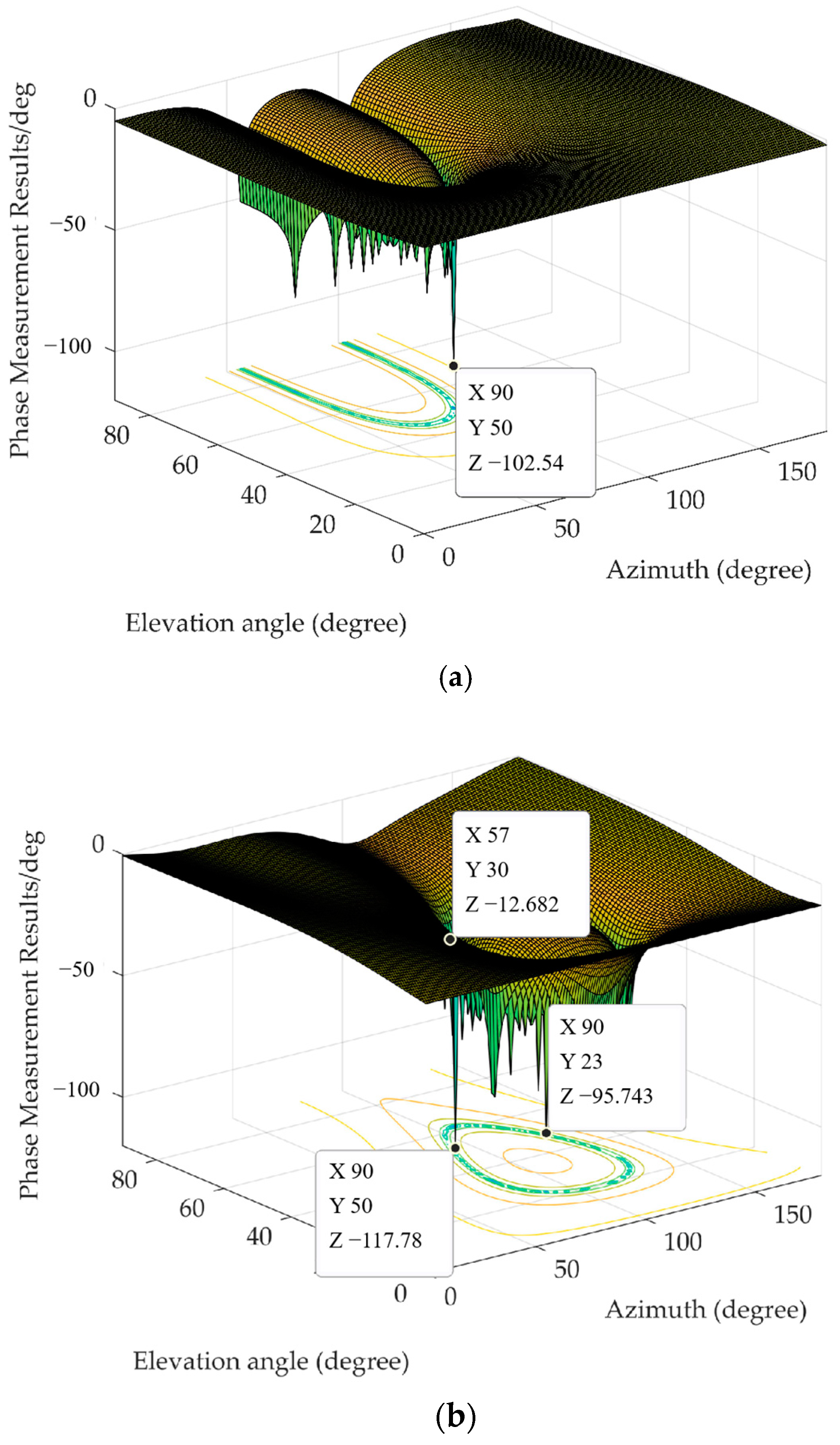
In the SAP PI algorithm, the phase biases of three-dimension distribution and two-dimension distribution are shown in Figure 7a,b. The phase bias ranges from to . When the direction of the interference signal is the same as the satellite signal, the phase bias is .
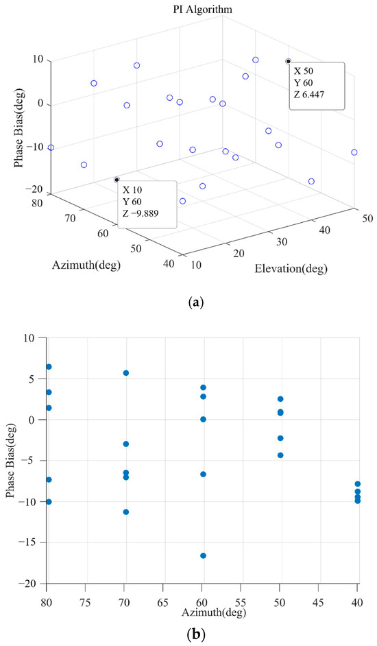
Figure 7.
The phase bias distributions of SAP PI algorithm: (a) three-dimension; (b) two-dimension.
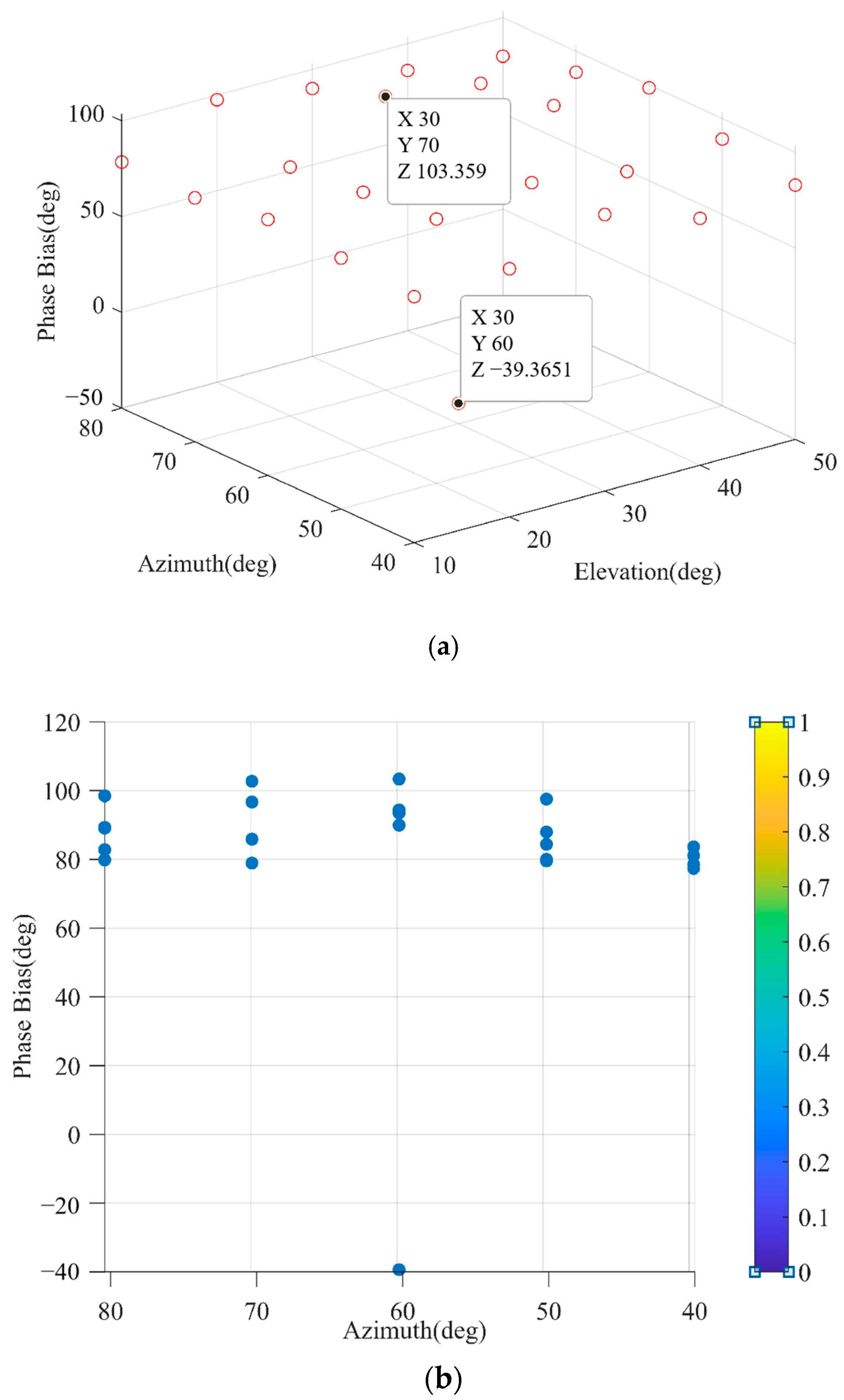
In the STAP PI algorithm, the phase biases of three-dimension distribution and two-dimension distribution are shown in Figure 8a,b. The phase bias ranges from to . When the direction of the interference signal is the same as the satellite signal, the phase bias is .
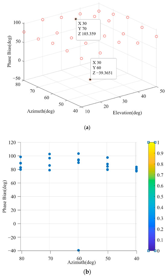
Figure 8.
The phase bias distributions of STAP PI algorithm: (a) three-dimension; (b) two-dimension.
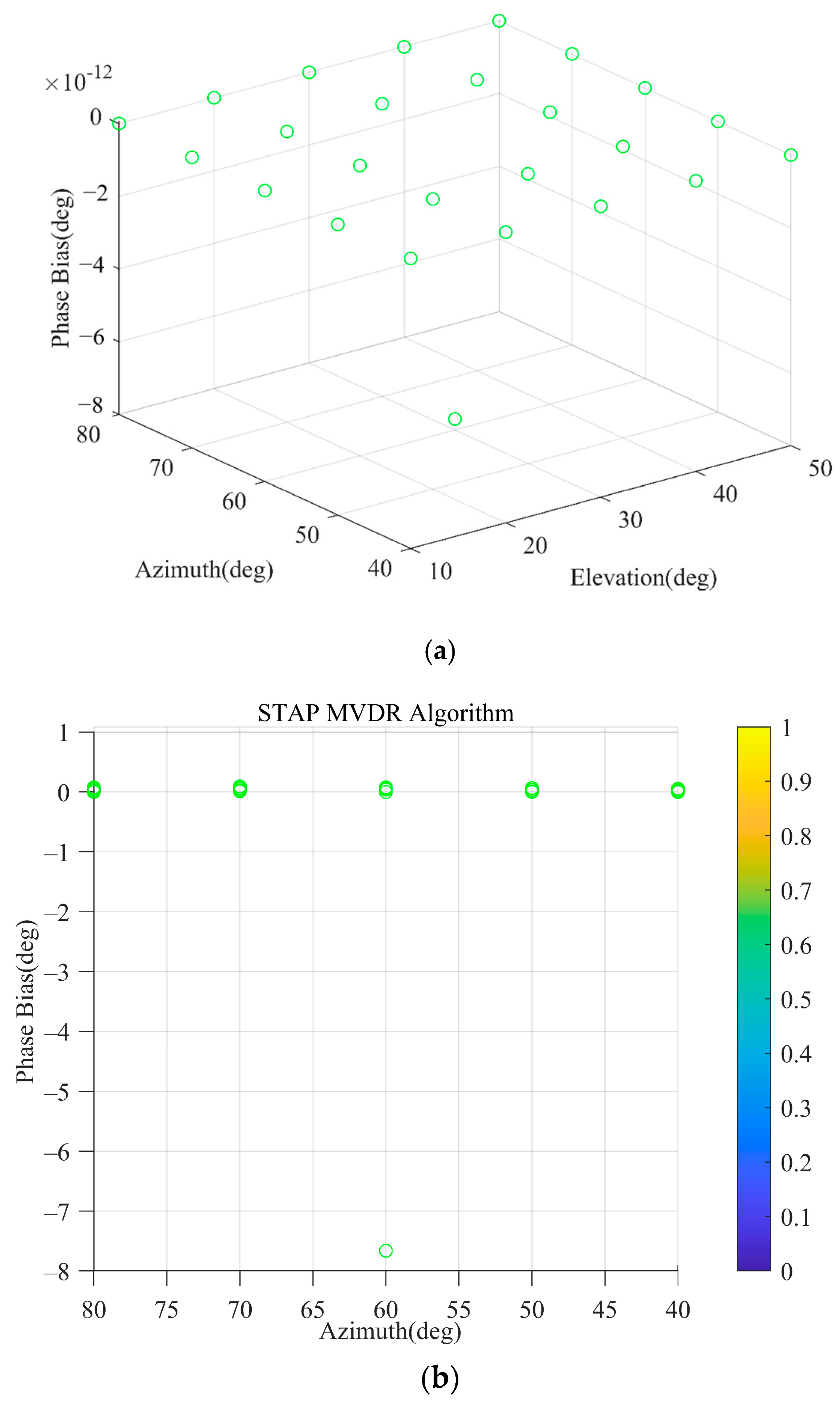
In the STAP MVDR algorithm, the phase biases of three-dimension distribution and two-dimension distribution are shown in Figure 9a,b. Based on the analysis of Section 2.5.1, the MVDR criterion will not introduce phase bias. Therefore, the phase bias in Figure 9 is .
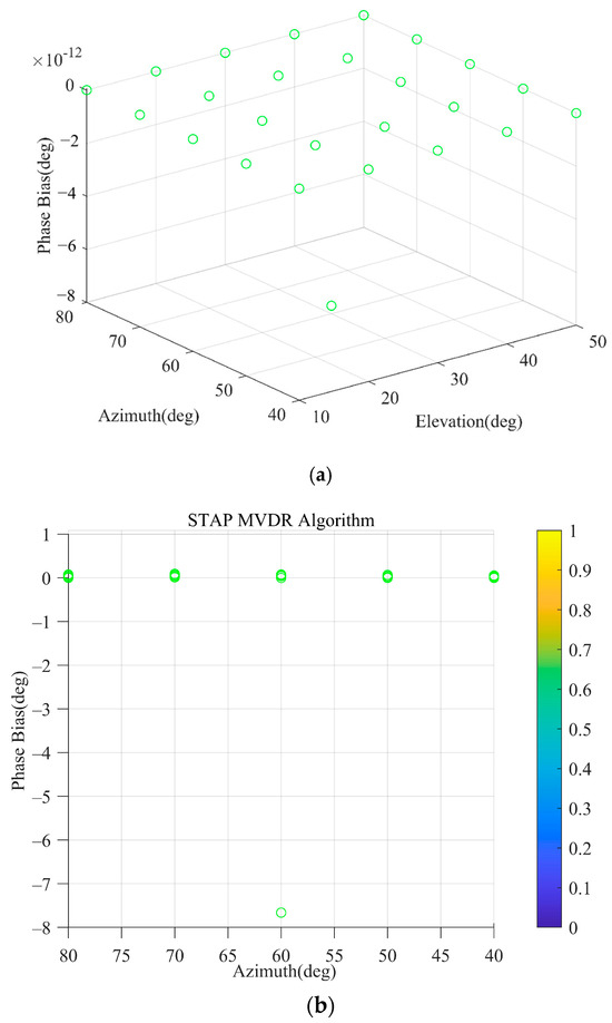
Figure 9.
The phase bias distributions of STAP MVDR algorithm: (a) three-dimension; (b) two-dimension.
3.2. The Performance of Anti-Interference Algorithm with Phase Bias Compensation
Assume the incident signal from . The RF is 1268.52 MHz, intermediate frequency (IF) is 46.52 MHz, and sampling frequency is 62 MHz. The carrier-to noise ratio (CNR) is 45 dB. A broadband interference signal is from , and the interference-to-noise ratio is 75 dB.
We take five- and seven-element antenna arrays as examples of odd-element arrays, and the weight coefficients are shown in Table 3. In Figure 10, the anti-interference performance of phase bias compensation is given.
Table 3.
Weight coefficients of bias compensation algorithm.
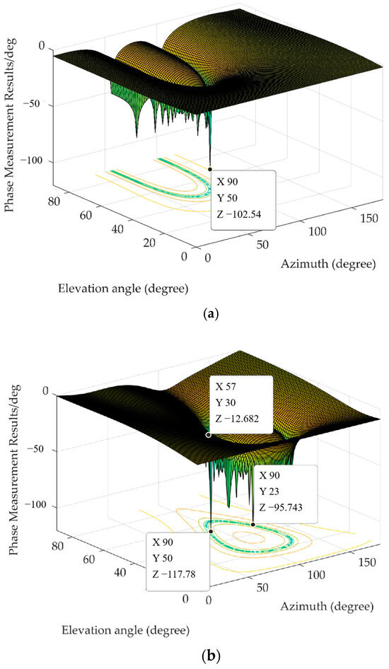
Figure 10.
Anti-interference performance of bias compensation algorithm: (a) 7 elements; (b) 5 elements.
The anti-interference algorithm with phase bias compensation creates a beam null in the direction of the interference, effectively suppressing the interference signals. However, it results in an approximately 10~12 dB attenuation of the useful signals, leading to a decrease in the output signal-to-noise ratio compared to the algorithm without bias compensation. Nevertheless, while the algorithm suppresses interference, it does so at the cost of signal-to-noise ratio loss without affecting the phase of the output signal, demonstrating the effectiveness of this algorithm.
4. Discussion
In this section, we discuss the phase compensation performance based on the tracking process of the GNSS receiver.
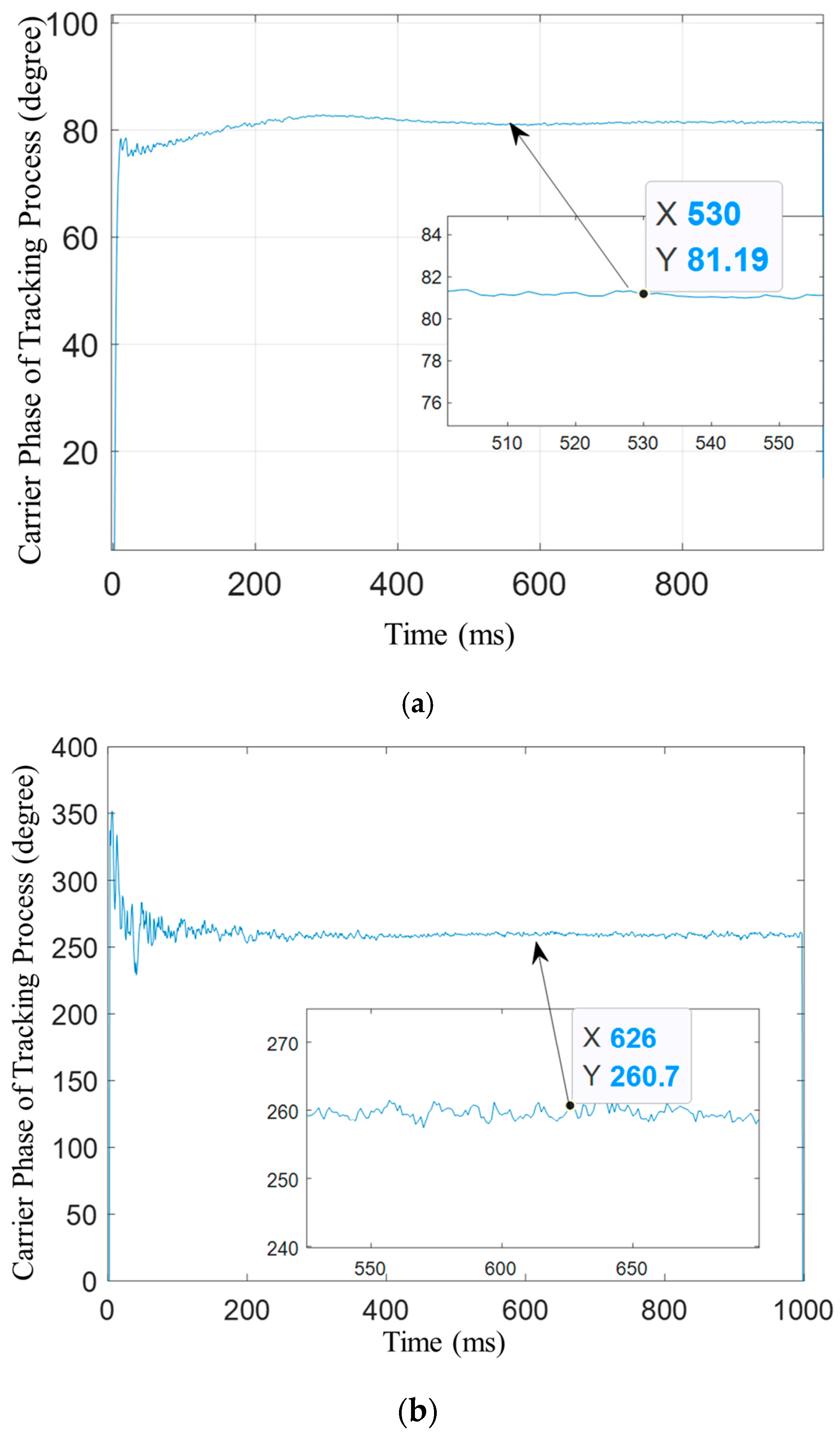
In Figure 11, we provide the carrier phase of the original satellite signal and the carrier phase after anti-interference algorithm processing. It can be observed that within one cycle, the phase bias from the original satellite signal is approximately 179.5°.
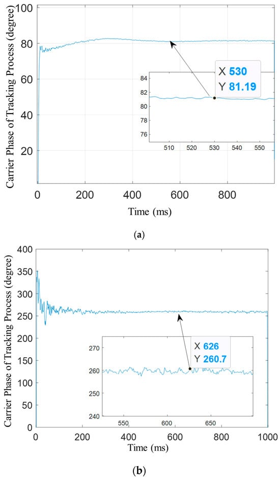
Figure 11.
The carrier phase tracking results for antenna array. (a) The original phase of satellite signal. (b) The carrier phase after anti-interference algorithm processing.
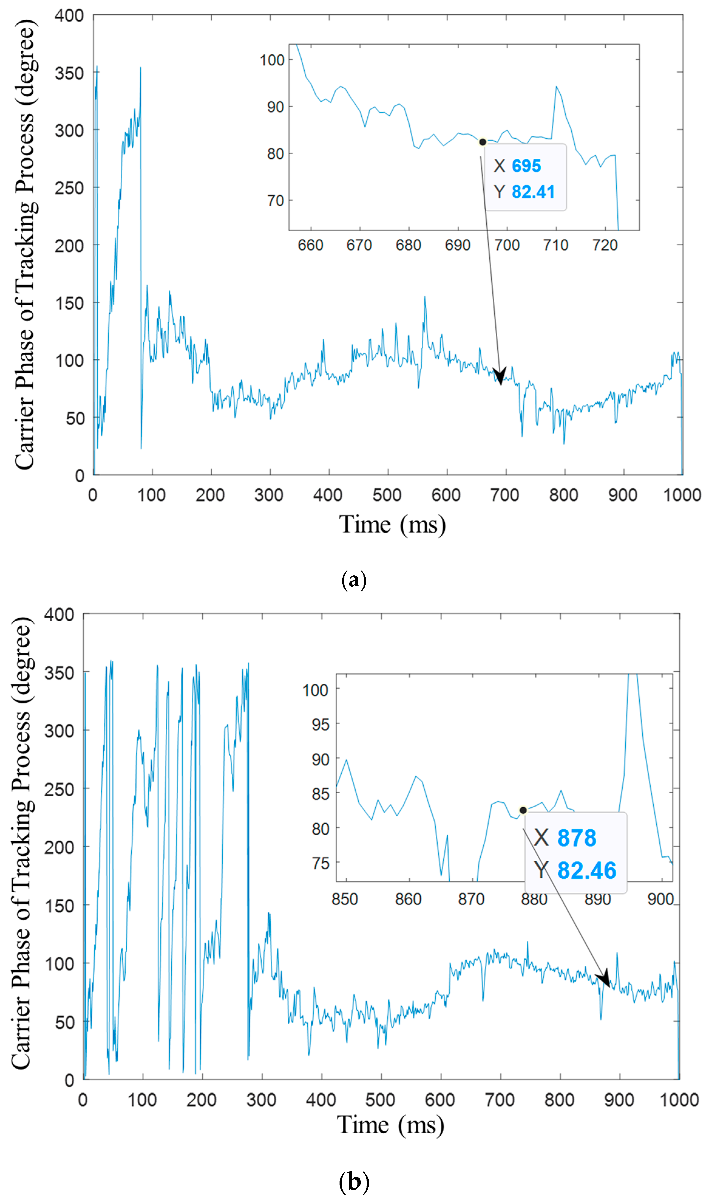
When the number of array elements is five or seven, the simulation results of the bias compensation method based on array weighted-coefficient conjugation are as follows. Figure 12a indicates the phase of the bias compensation method based on array weighted-coefficient conjugation when the number of antenna elements is five and Figure 12b indicates the phase bias compensation results when the number of antenna elements is seven. Only when the operating time is over 700 ms does the carrier phase approximate that of the original desired signal. When the rough compensation can meet the phase measurement accuracy requirements, the user can adopt the results. However, when users have higher requirements for phase measurement accuracy and stability, they need to use fine compensation to increase the accuracy.
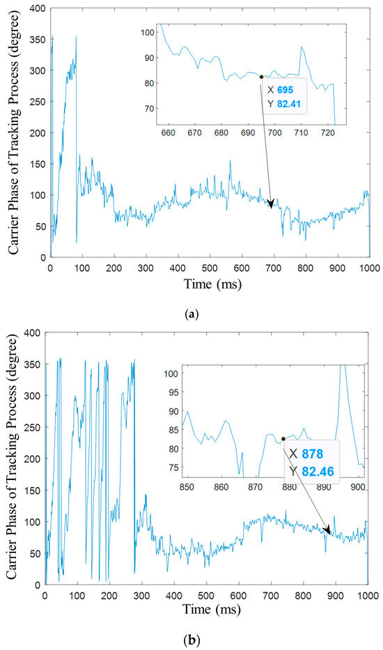
Figure 12.
The phase of bias compensation method based on array weighted-coefficient conjugation: (a) 5 antenna elements; (b) 7 antenna elements.
In Figure 13, we provide the phase bias compensation results at the anti-interference output signal. The difference between the output signal and the original satellite signal is only 2°.
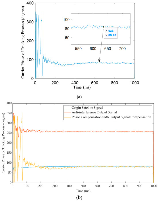
Figure 13.
The phase of bias compensation at anti-interference output signal: (a) phase compensation with output signal compensation; (b) comparison of signals before and after phase compensation.
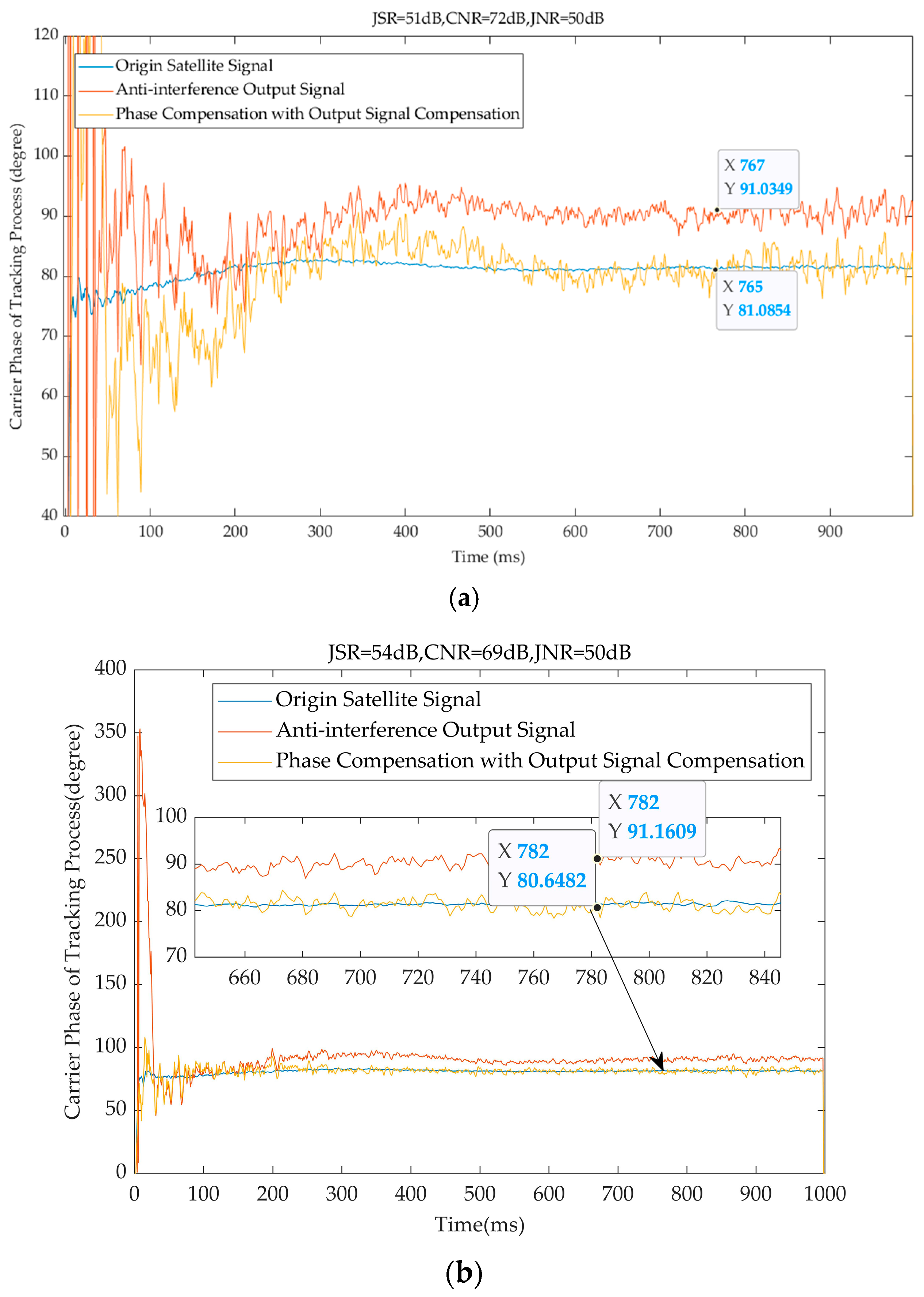
The simulation scenario of Figure 13 is established with the jammer-to-signal ratio (JSR) of 48 dB. Therefore, we analyze the effectiveness of the compensation algorithm at different JSR values. Simulation experiments are conducted with JSRs set to 51 dB and 54 dB.
As shown in Figure 14a, with a JSR of 51 dB and a carrier-to-noise ratio (CNR) of 72 dB, the carrier phase of the original satellite signal is around 82°, while the carrier phase of the output signal after anti-interference is approximately 91°, introducing a deviation of about 9°. After applying the compensation algorithm, the mean phase bias is reduced to 0.23°, and the variance phase bias is 2.77°.
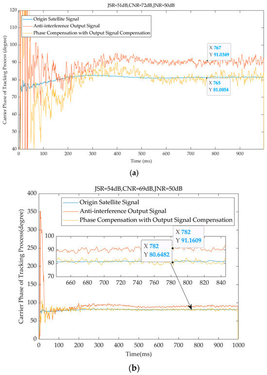

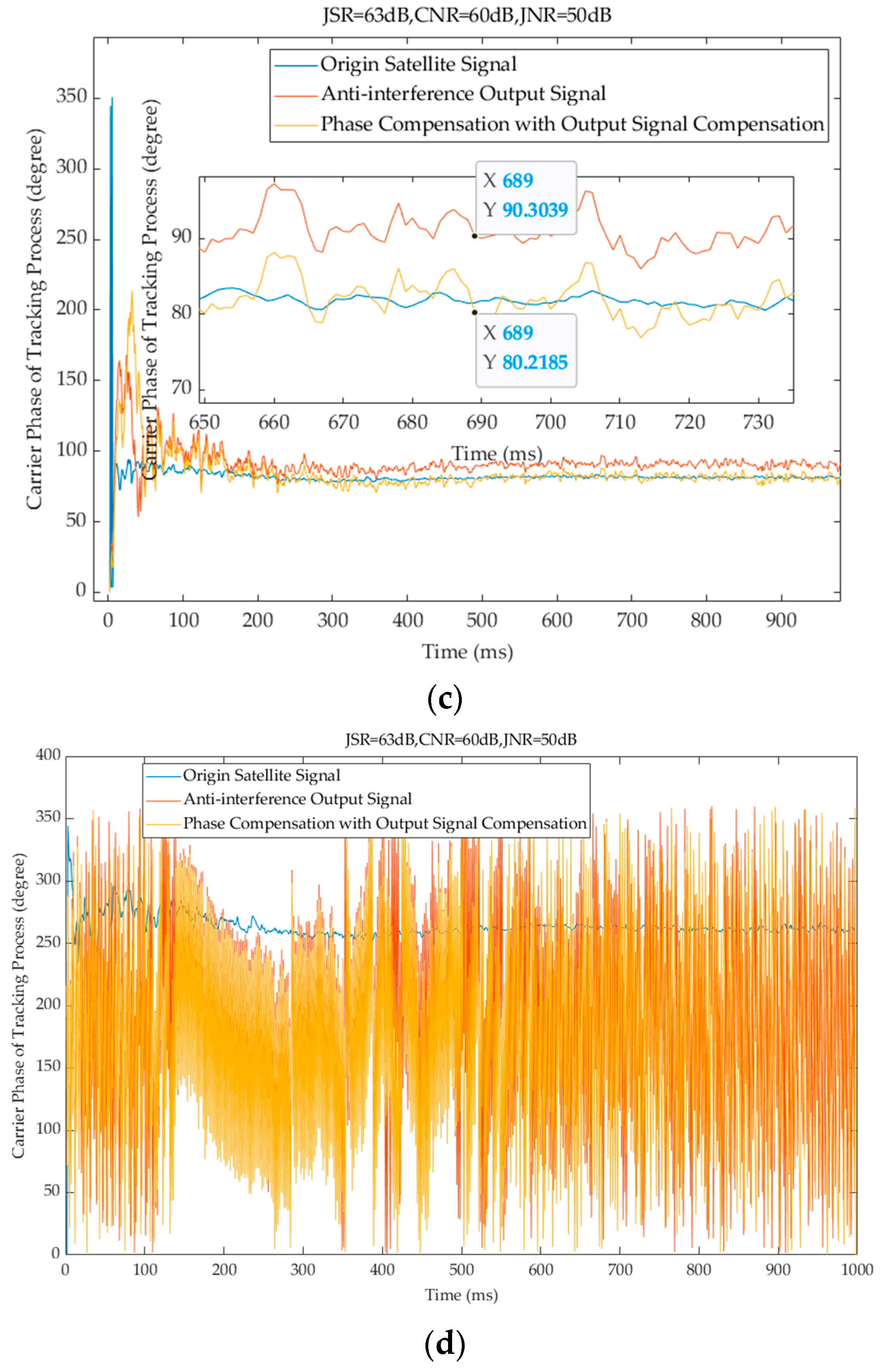
Figure 14.
The phase bias compensation at different JSR values. (a) JSR = 51 dB. (b) JSR = 54 dB. (c) JSR = 63 dB. (d) JSR = 73 dB.
In Figure 14b, with a JSR of 54 dB, a CNR of 69 dB, and a jammer-to-noise ratio (JNR) of 50 dB, the situation is similar to that of a JSR of 51 dB. Anti-interference introduces a bias of 8.6°, but the compensation algorithm can keep the mean phase bias within 0.04° and the variance phase bias within 2.41°.
In Figure 14c, with a JSR of 63 dB, CNR of 60 dB, and JNR of 50 dB, the compensation algorithm similarly achieves the desired compensation effect. After the phase bias compensation, the mean phase bias is reduced to 0.25°, and the variance phase bias is 4.62°.
In Figure 14d, with a JSR of 73 dB, CNR of 50 dB, and JNR of 50 dB, it is impossible to achieve compensation with the anti-interference algorithm.
Table 4 shows that the phase bias compensation consistently reduces the mean phase bias to near-zero levels across all JSR and CNR conditions, indicating effective compensation. However, the variance of phase bias generally increases after compensation, suggesting some variability in the compensation process, which may need further investigation or optimization. Moreover, with JSR increases and CNR decreases, the mean phase bias in the anti-interference stage increases, indicating higher interference levels. The compensation stage remains effective in reducing the mean phase bias, but the variance remains a concern.
Table 4.
The comparison of phase bias compensation results.
5. Conclusions
This paper has proposed a two-step phase bias compensation method for anti-interference antenna arrays consisting of rough bias compensation (based on array weighted-coefficient conjugation) and fine bias compensation (applied to the anti-interference output signal). Compared to the conventional MVDR algorithm, our approach achieves a significant improvement in angular accuracy with a simplified structure and lower engineering cost. There are two key contributions in the paper. First, under the simulated conditions of JSR = 63 dB, CNR = 60 dB, and JNR = 50 dB, the mean phase bias is reduced to 0.25°, and the variance phase bias is reduced to 4.62°. At the situation where CNR ≥ 60 dB, the method can compensate the phase bias successfully. Second, the two-step compensation architecture eliminates the need for complex real-time calibration, enabling high-precision positioning (via PI algorithm integration) while maintaining computational efficiency. However, this paper has not considered the error due to mutual coupling between array elements. In the applications of small arrays and receiver positioning, this omission would theoretically affect the accuracy of phase bias compensation. In the future work, we will analysis the influence of mutual coupling and extend this framework to multi-band scenarios.
Author Contributions
Methodology, J.Z.; software, J.Z.; validation, J.Z.; formal analysis, J.Z. and W.F.; investigation, W.F.; resources, W.F.; data curation, W.F.; writing—original draft, J.Z. and H.W.; writing—review and editing, J.Z.; visualization, H.W.; supervision, H.W.; project administration, H.W. All authors have read and agreed to the published version of the manuscript.
Funding
This research was funded by the National Key R&D Program of China, grant number 2024YFC3015605.
Data Availability Statement
The data presented in this study are available on request from the corresponding author due to privacy restrictions.
Conflicts of Interest
The authors declare no conflicts of interest.
References
- Li, X.; Li, X.; Huang, J. Improving PPP–RTK in Urban Environment by Tightly Coupled Integration of GNSS and INS. J. Geod. 2022, 95, 132. [Google Scholar] [CrossRef]
- Zhang, B.; Hou, P.; Zha, J.; Liu, T. PPP–RTK Functional Models Formulated with Undifferenced and Uncombined GNSS Observations. Satell. Navig. 2022, 3, 3–15. [Google Scholar] [CrossRef]
- Han, S.; Han, D. Enhancing Direct Georeferencing Using Real-Time Kinematic UAVs and Structure from Motion-Based Photogrammetry for Large-Scale Infrastructure. Drones 2024, 8, 736. [Google Scholar] [CrossRef]
- Craven, P.; Wong, R.; Fedora, N.; Crampton, P. Studying the effects of interference on GNSS signals. In Proceedings of the 2013 International Technical Meeting of the Institute of Navigation, San Diego, CA, USA, 27–29 January 2013; pp. 186–893. [Google Scholar]
- Huang, L.; Lu, Z.; Xiao, Z.; Ren, C.; Song, J.; Li, B. Suppression of jammer multipath in GNSS antenna array receiver. Remote Sens. 2022, 14, 350. [Google Scholar] [CrossRef]
- Broumandan, A.; Jafarnia-Jahromi, A.; Daneshmand, S.; Lachapelle, G. Overview of spatial processing approaches for GNSS structural interference detection and mitigation. Proc. IEEE 2016, 104, 1246–1257. [Google Scholar] [CrossRef]
- Yang, X.; Wang, F.; Liu, W.; Chen, F. A new blind anti interference algorithm based on a novel antenna array design. IET Radar Sonar Navig. 2022, 16, 1616–1626. [Google Scholar] [CrossRef]
- Shaw, A.; Jared, S.; Aboulnasr, H. MVDR Beamformer Design by Imposing Unit Circle Roots Constraints for Uniform Linear Arrays. IEEE Trans. Signal Process. 2021, 69, 6116–6130. [Google Scholar] [CrossRef]
- Lin, T.; Cong, J.; Zhu, Y.; Zhang, J.; Ben Letaief, K. Hybrid Beamforming for Millimeter Wave Systems Using the MMSE Criterion. IEEE Trans. Commun. 2019, 67, 3693–3708. [Google Scholar] [CrossRef]
- Yang, X.; Yin, P.; Zeng, T.; Sarkar, T.K. Applying Auxiliary Array to Suppress Mainlobe Interference for Ground-Based Radar. IEEE Antennas Wirel. Propag. Lett. 2013, 12, 433–436. [Google Scholar] [CrossRef]
- Fertig, L. Analytical approximations for Space-Time Adaptive Processing (STAP) performance. In Proceedings of the 2014 IEEE Radar Conference, Cincinnati, OH, USA, 19–23 May 2014; pp. 122–125. [Google Scholar]
- Sun, Y.; Xie, J.; Gong, Y.; Zhang, Z.; Wang, L. Adaptive Interference Mitigation Space-Time Array Reconfiguration by Joint Selection of Antenna and Delay Tap. IET Radar Sonar Navig. 2024, 18, 448–462. [Google Scholar] [CrossRef]
- Cheng, Q.; Hua, Y.; Stoica, P. Asymptotic performance of optimal gain-and-phase estimators of sensor arrays. IEEE Trans. Signal Process. 2000, 48, 3587–3590. [Google Scholar]
- Otaru, M.U.; Zerguine, A.; Cheded, L. Adaptive channel equalization: A simplified approach using the quantized-LMF algorithm. In Proceedings of the 2008 IEEE International Symposium on Circuits and Systems (ISCAS), Seattle, WA, USA, 18–21 May 2008; pp. 1136–1139. [Google Scholar]
- Xie, Y.; Chen, F.; Huang, L.; Liu, Z.; Wang, F. Carrier Phase Bias Correction for GNSS Space-Time Array Processing Using Time-Delay Data. GPS Solut. 2023, 27, 113. [Google Scholar] [CrossRef]
- Cao, K.; Wang, L.; Li, B.; Ma, H. A Real-Time Phase Center Variation Compensation Algorithm for the Anti interference GNSS Antennas. IEEE Access 2020, 8, 128705–128715. [Google Scholar] [CrossRef]
- Kim, U.S. Mitigation of Signal Biases Introduced by Controlled Reception Pattern Antennas in a High Integrity Carrier Phase Differential GPS System. Ph.D. Thesis, Stanford University, Stanford, CA, USA, 2007. [Google Scholar]
- Brien, J.O.; Gupta, I.J. Mitigation of Adaptive Antenna Induced Bias Errors in GNSS Receivers. IEEE Trans. Aerosp. Electron. Syst. 2011, 47, 524–538. [Google Scholar]
- Jia, Q.; Wu, R.; Wang, W.; Lu, D.; Wang, L. Adaptive blind anti-jamming algorithm using acquisition information to reduce the carrier phase bias. GPS Solut. 2018, 22, 99. [Google Scholar] [CrossRef]
- Wang, Y.; Liu, W.; Huang, L.; Xiao, Z.; Wang, F. Distortionless Pseudo-Code Tracking Space–Time Adaptive Processor Based on the PI Criterion for GNSS Receiver. IET Radar Sonar Navig. 2020, 14, 1984–1990. [Google Scholar] [CrossRef]
- Li, S.; Wang, F.; Tang, X.; Ni, S.; Lin, H. Anti-Jamming GNSS Antenna Array Receiver with Reduced Phase Distortions Using a Robust Phase Compensation Technique. Remote Sens. 2023, 15, 4344. [Google Scholar] [CrossRef]
- An, Y.; Kang, R.L.; Ban, Y.L.; Yang, S.S. Beidou Receiver Based on Anti-Jamming Antenna Arrays with Self-Calibration for Precise Relative Positioning. J. Syst. Eng. Electron. 2024, 35, 1132–1147. [Google Scholar] [CrossRef]
- Wang, J.; Liu, W.; Chen, F.; Lu, Z.; Ou, G. GNSS array receiver faced with overloaded interferences: Anti-jamming performance and the incident directions of interferences. Journal of Systems Engineering and Electronics. J. Syst. Eng. Electron. 2023, 34, 335–341. [Google Scholar] [CrossRef]
- Wu, J.; Tang, X.; Huang, L.; Ni, S.; Wang, F. Blind adaptive beamforming for a global navigation satellite system array receiver based on direction lock loop. Remote Sens. 2023, 15, 3387. [Google Scholar] [CrossRef]
- Fertig, L.B. Analytical Expressions for Space-Time Adaptive Processing (STAP) Performance. IEEE Trans. Aerosp. Electron. Syst. 2015, 51, 42–53. [Google Scholar] [CrossRef]
- Sun, Y.; Chen, F.; Lu, Z.; Wang, F. Anti interference Method and Implementation for GNSS Receiver Based on Array Antenna Rotation. Remote Sens. 2022, 14, 4774. [Google Scholar] [CrossRef]
- Jin, Y.; Zhang, H.; Lu, T.; Yang, H.; Gulliver, T.A. A Novel Power Inversion Antenna Array for the Beidou Navigation Satellite System. IEEE Access 2019, 7, 25382–25397. [Google Scholar] [CrossRef]
- Xiao, Y.; Yin, J.; Qi, H.; Yin, H.; Hua, G. MVDR Algorithm Based on Estimated Diagonal Loading for Beamforming. Math. Probl. Eng. 2017, 2017, 7904356. [Google Scholar] [CrossRef]
- Zhang, H. A LiDAR–INS-Aided Geometry-Based Cycle Slip Resolution for Intelligent Vehicle in Urban Environment with Long-Term Satellite Signal Loss. GPS Solut. 2024, 28, 61–80. [Google Scholar] [CrossRef]
- Xue, L.; Li, X.; Wu, W.; Wang, L.; Zhang, J. The Uplink VLBI Receiving System for Deep Space Exploration in the Spacecraft. IEEE Trans. Instrum. Meas. 2024, 73, 8507711. [Google Scholar]
- Shu, B. Performance Analysis of BDS Medium-Long Baseline RTK Positioning Using an Empirical Troposphere Model. Sensors 2018, 18, 1199. [Google Scholar] [CrossRef]
- Choi, B.K.; Su, Y.H.; Jeong, L.S. Performance Analysis of Long Baseline Relative Positioning using Dual-frequency GPS/BDS Measurements. J. Position. Navig. Timing 2019, 8, 87–94. [Google Scholar]


Disclaimer/Publisher’s Note: The statements, opinions and data contained in all publications are solely those of the individual author(s) and contributor(s) and not of MDPI and/or the editor(s). MDPI and/or the editor(s) disclaim responsibility for any injury to people or property resulting from any ideas, methods, instructions or products referred to in the content. |
© 2025 by the authors. Licensee MDPI, Basel, Switzerland. This article is an open access article distributed under the terms and conditions of the Creative Commons Attribution (CC BY) license (https://creativecommons.org/licenses/by/4.0/).