Article

VibrantVS: A High-Resolution Vision Transformer for Forest Canopy Height Estimation

Vibrant Planet, Public Benefit Corporation, 11025 Pioneer Trail Suite 200A, Truckee, CA 96161, USA
*
Author to whom correspondence should be addressed.
Remote Sens. 2025, 17(6), 1017; https://doi.org/10.3390/rs17061017
Submission received: 22 January 2025 / Revised: 8 March 2025 / Accepted: 11 March 2025 / Published: 14 March 2025

Abstract

:
This paper explores the application of a novel vision transformer (ViT) model for the estimation of canopy height models (CHMs) using 4-band National Agriculture Imagery Program (NAIP) imagery across the western United States. We compare the effectiveness of this model in terms of accuracy and precision aggregated across ecoregions and class heights versus three other benchmark peer-reviewed models. Key findings suggest that, while other benchmark models can provide high precision in localized areas, the VibrantVS model has substantial advantages across a broad reach of ecoregions in the western United States, with higher accuracy, higher precision, the ability to generate updated inference at a cadence of three years or less, and high spatial resolution. The VibrantVS model provides significant value for ecological monitoring and land management decisions, including for wildfire mitigation.

1. Introduction

During the past three decades, increases in the number of wildfires and burned areas across the western United States have negatively impacted human health, assets, and ecological structure and function [1,2]. This fire activity, compounded by recent widespread drought and historic fire suppression [3], has led to forest conditions that lack sufficient resilience to recover from natural disturbances and thereby threaten the ecosystem services on which human communities depend [4,5]. Such conditions have required forest managers to prioritize the restoration of historical fire regimes and the treatment and maintenance of forests to reduce the potential for high-severity fire [6]. A major requirement in the identification of appropriate treatments and restoration actions is access to current spatial data that accurately describes the horizontal and vertical structure of vegetation.
Canopy height models (CHMs) describe the height of the canopy top from the ground. The availability of current canopy height data in a three-dimensional georeferenced surface [7] is crucial for various ecological applications, including biomass estimation [8], predicting fire behavior [9,10], individual tree detection [11,12], and habitat quality assessment [13]. Accurate quantification of canopy height not only enhances our understanding of forest dynamics [14,15,16] but also facilitates strategic, tactical, and operational planning decisions to improve forest health, promote biodiversity, and protect threatened and endangered species [17]. Therefore, the development of a high-resolution continuous CHM across large (in excess of 1 million ha), multi-jurisdictional landscapes such as the western United States is critical for the successful restoration, monitoring, and management of forests.
Lidar has emerged as the gold standard for the three-dimensional mapping of vegetation structure due to its high spatial fidelity and ability to penetrate forest canopies [14,18,19]. However, even with economies of scale [20] and cost effectiveness compared to conducting field inventories over large areas [8], lidar datasets are constrained by their limited spatial and temporal coverage. These constraints limit the ability of lidar acquisitions to reflect up-to-date forest structure because of the dynamic nature of forest ecosystems as they respond to disturbances, treatments, natural growth, or climate change [21]. On the other hand, the proliferation of freely available, remotely sensed data with consistent temporal revisit periods, such as the satellite-based imagery of Sentinel-2 [22], or aerial imagery from NAIP, has opened new avenues to methodologies that can be tailored to model vegetation structure with high spatial and temporal resolution over longer periods of time and over larger areas [23,24].
The availability of large remotely sensed image libraries in conjunction with newer deep-learning methods has allowed for the emergence of a suite of modeled canopy height products providing continuous high-resolution (1–30 m) forest structure measurements across broad spatial extents [25,26,27]. This paper aims to benchmark a selection of the latest peer-reviewed deep-learning/machine-learning-based CHMs across varied ecosystems in the western United States. Additionally, we describe our own vision transformer model based on NAIP imagery as an input: VibrantVS. We present an analysis that will (1) address which model is optimal based on standard machine-learning metrics compared to aerial lidar measurements to serve as a benchmark for the broad remote sensing community, and (2) compare model estimates across a variety of ecoregions in the western United States to better understand the utility of these models for fine-grained ecological management and decision-making.

2. Materials and Methods

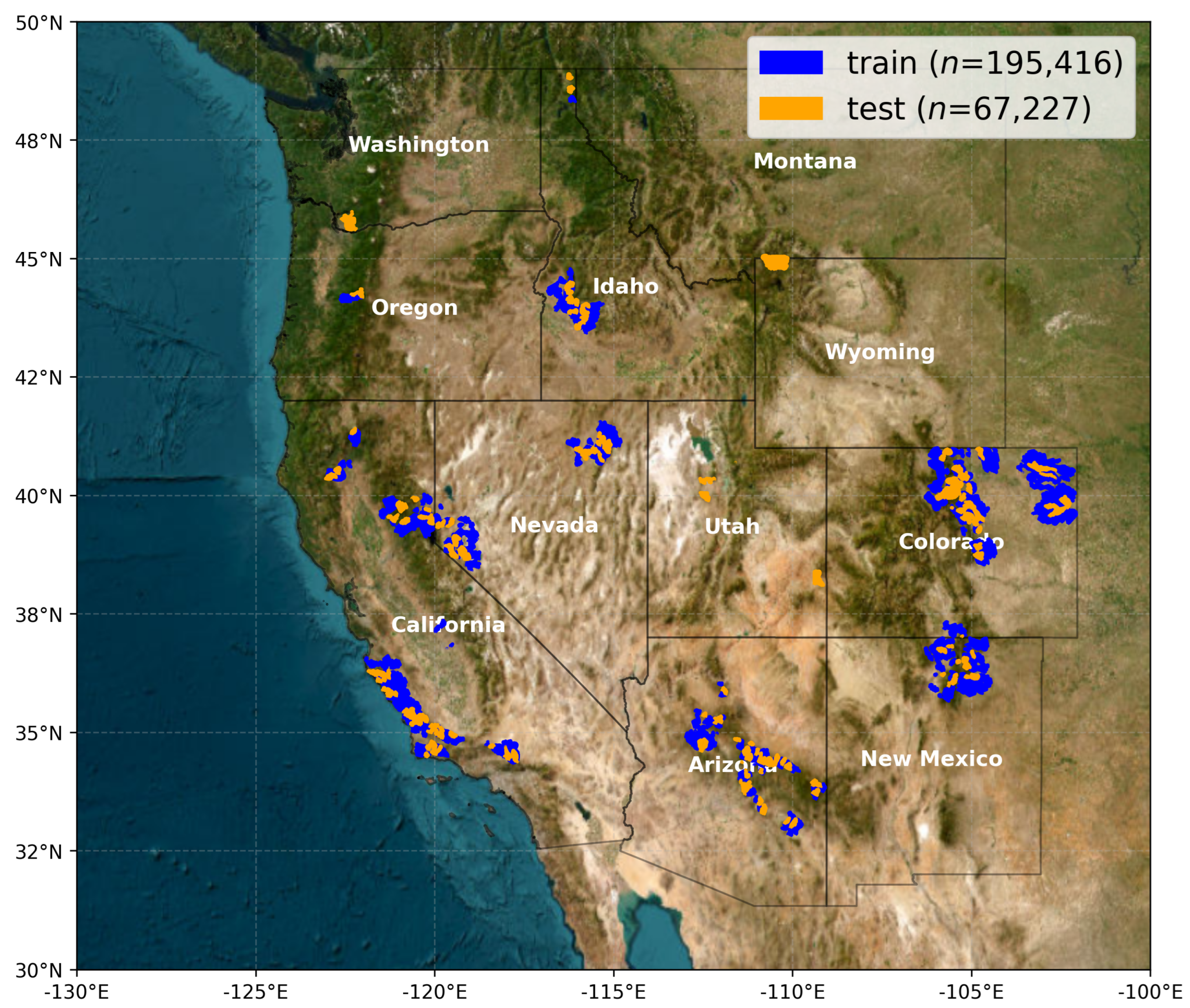
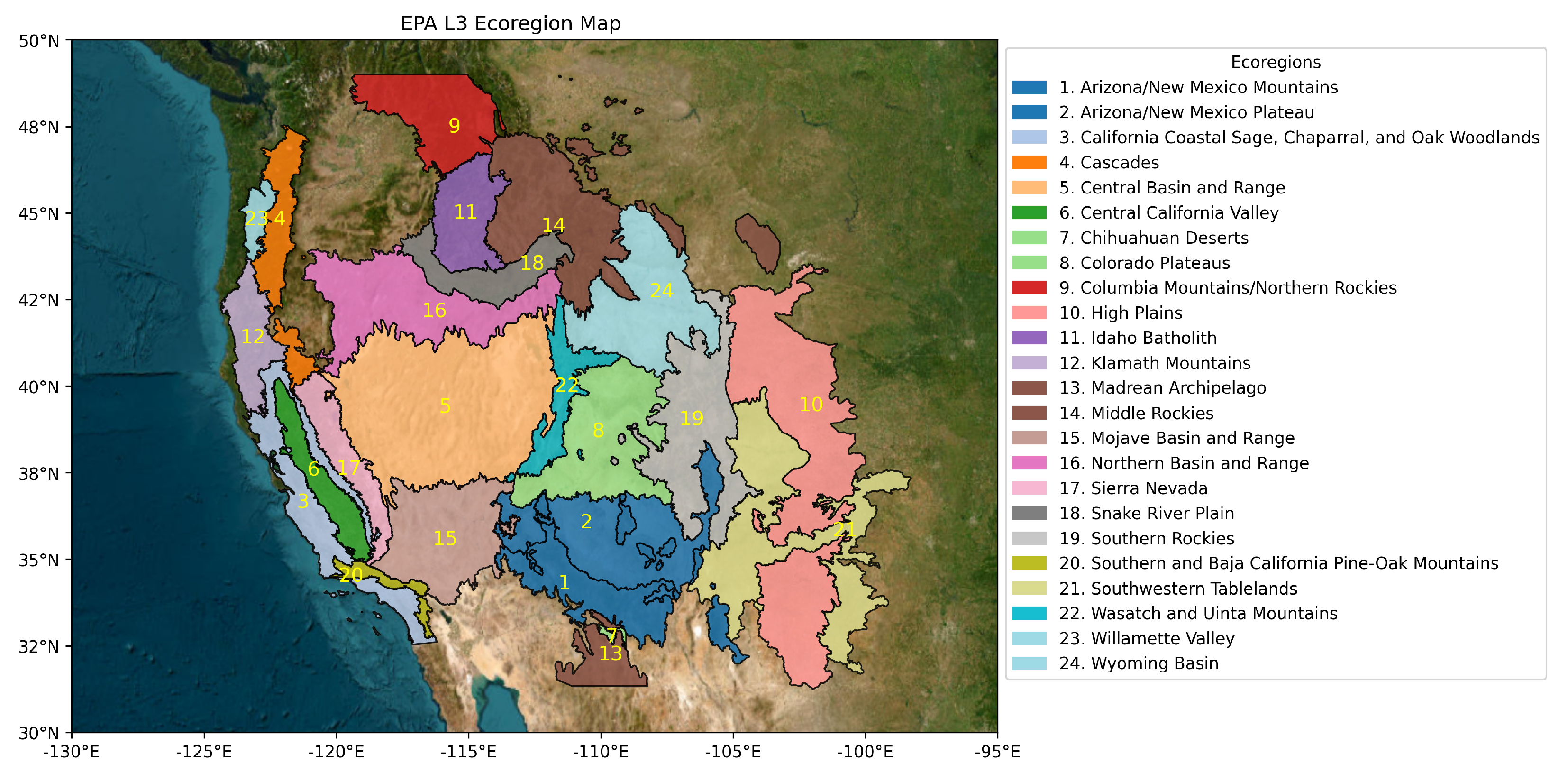
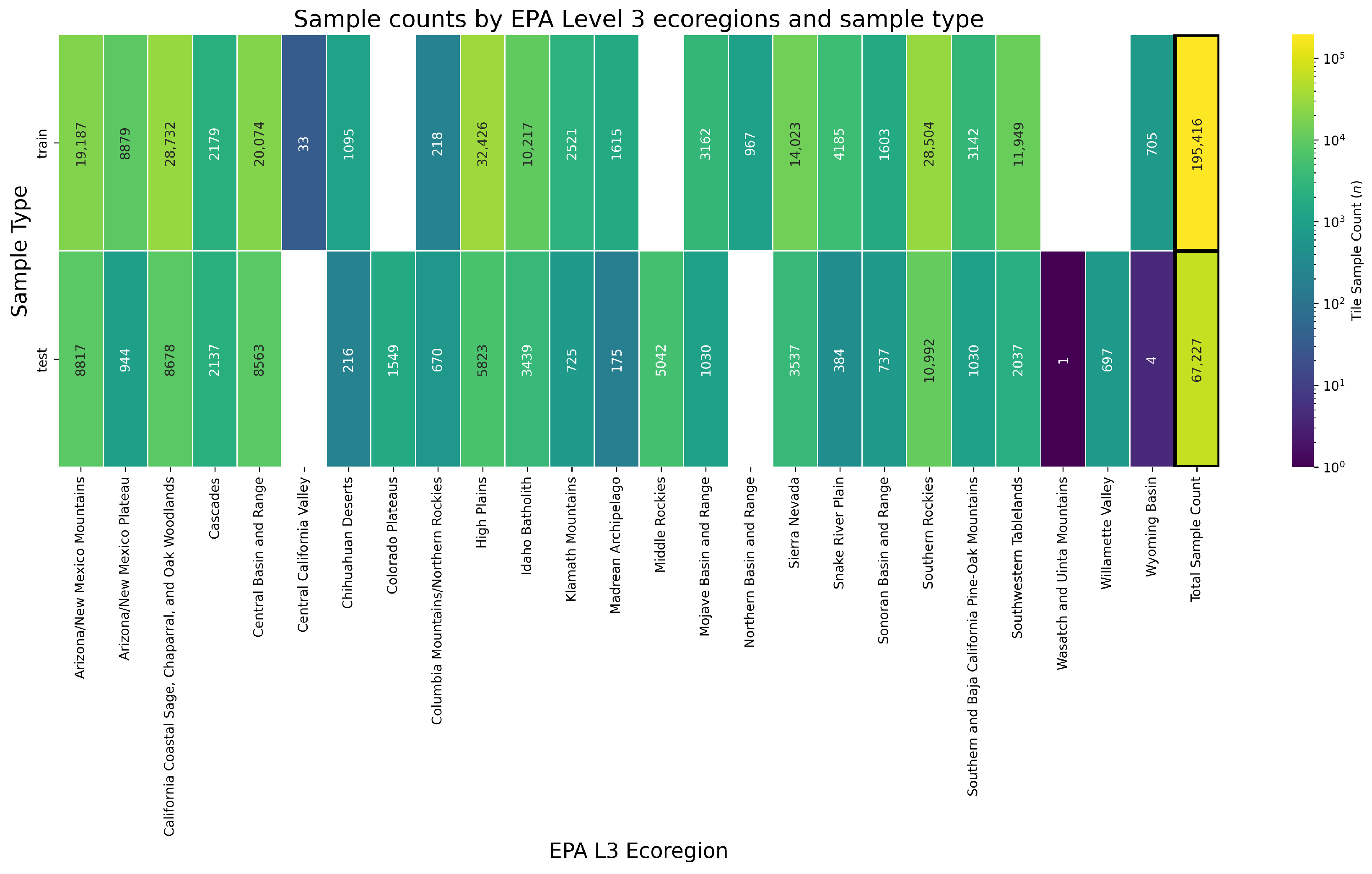
2.1. Study Area and Data

In this study, we compare CHMs for the western contiguous United States. Given our focus on forest structure data that would have the greatest utility in understanding wildfire impacts, we focus our sampling to intersect the following (Figure 1):
  • The Wildfire Crisis Strategy (WCS) landscapes defined by the United States Forest Service (USFS) to prioritize regions at the greatest risk of severe wildfire [28].
  • National Ecological Observatory Network (NEON) research sites within the western United States, due to their independent collection of individual field-based tree-height measurements and aerial lidar against which to validate model predictions [29].
  • Areas that intersect the spatial extent for the 3D Elevation Program (3DEP) work units in the Work Unit Extent Spatial Metadata (WESM) dataset [30] that meet the seamless and 1 m DEM quality criteria.
Figure 1. Sampling of tiles within Hydrologic Units 12 (HUC12) watersheds of the western United States that covers 24 EPA L3 ecoregions containing sufficient quality 3DEP lidar data and spatially/temporally intersecting NAIP data. Regions were additionally selected within WCS areas to optimize for model evaluation in regions where wildfire risk mitigation is a priority.
Remotesensing 17 01017 g001
To quantify the ability of the models to robustly predict forest canopy height across an ecological gradient, we stratify our data by Environmental Protection Agency (EPA) Level 3 (L3) ecoregions [31] (Figure 2). EPA L3 ecoregions are delineated based on relatively homogeneous environmental conditions, such as vegetation types, soil, climate, and landforms. This coherence reduces variability in environmental factors unrelated to canopy height within each ecoregion, making it easier to evaluate the performance of the baseline models across a well-defined set of environmental conditions. Additionally, EPA L3 ecoregions provide a manageable range of dominant species and climate variability while still capturing key regional distinctions. Finally, evaluating CHM performance at this ecoregion scale can directly inform practices in forest management, carbon accounting, and biodiversity conservation.
We generated a total of 262,643 sample tiles with a spatial footprint of 0.5 × 0.5 km2 (1000 × 1000 pixel rasters at 0.5 m resolution) that crossed a total of 24 different EPA L3 ecoregions, providing us with a robust representation of tree vegetation data and lidar CHM heights (Figure A1). To ensure broad ecological diversity in model training, we randomly selected sample tiles while enforcing balanced representation across the 24 ecoregions (Figure 3). This stratified sampling approach prevents overrepresentation of highly sampled regions and ensures that all ecoregions contribute meaningfully to model training and evaluation. We split the data into two groups: (1) a training set of 195,416 samples, which contains data for training and validation of the VibrantVS ViT model; (2) a test set of 67,227 samples, which contain tiles withheld from the model to evaluate performance. The lidar collection dates range from 2014 to 2021 (Table 1).
To ensure consistency in training and evaluation, each sample was composed of a matched NAIP and aerial lidar CHM sample. Each NAIP sample was spatially and temporally paired with its corresponding lidar CHM. Spatial pairing was conducted by intersecting NAIP imagery tiles with the matching lidar acquisition footprint, while temporal pairing ensured that each NAIP tile was acquired within one year prior of the corresponding lidar dataset. This alignment reduces inconsistencies arising from vegetation growth, land cover changes, or disturbances such as wildfires, allowing the model to learn from accurate and time-matched canopy height labels. These carefully curated NAIP–lidar pairs were then distributed across the training and test sets to ensure robust generalization across diverse forested landscapes.

2.2. Predictor Data

NAIP Imagery

We utilized 4-band NAIP imagery, which includes RGB and near-infrared (NIR) bands [32]. These NAIP images are standard 4-band orthorectified aerial imagery and not stereoscopic in nature. To ensure consistency across training, validation, and inference datasets, we obtained NAIP imagery from the AWS Open Data Registry [33]. NAIP data are collected at the state level at varying temporal frequencies (originally at five-year cycles and every three years or less since 2009) and at varying spatial resolutions from 0.3 m to 1 m since the year 2002 to the present. To create uniform training, test, and inference datasets, we collected data from the AWS Open Data Registry [33] and preprocessed the data for the years 2014–2022. The preprocessing steps included the following:
  • Resampling all images to a uniform spatial resolution of 0.5 m using bilinear interpolation to ensure consistency across different acquisition years and states.
  • Tiling the images into standardized 1 × 1 km2 spatial footprint tiles for efficient storage and processing.
  • Storing processed imagery in AWS S3 storage buckets using the Cloud-Optimized GeoTIFF (COG) format to facilitate fast retrieval and scalable cloud-based processing.
  • Filtered NAIP tile data to be within one year prior of the spatially coincident lidar acquisition date to reduce opportunities for incorrect labels for the same tile due to disturbances such as wildfires.
These preprocessing steps ensure that the NAIP data used in our study maintain spatial, spectral, and temporal consistency, thereby improving the robustness and accuracy of model training and inference.

2.3. Label Data

3DEP Lidar

We downloaded available lidar data developed by the USGS 3DEP program [34]. All lidar geospatial metadata are available by work unit in the Work Unit Extent Spatial Metadata (WESM) GeoPackage that is published daily [30]. The WESM contains information about lidar point clouds and which source digital elevation model (DEM) work units have been processed and made available to the public. It includes metadata about work units, including quality level, data acquisition dates, and links to project-level metadata. To ensure consistency in data quality and spatial alignment, we applied a series of preprocessing steps to standardize the lidar data before model training. We developed automated scripts using the ‘lidR’ package version 4.1.2 in R version 4.4.0 [35] to systematically retrieve, process, and tile lidar data for efficient storage and analysis. The processing steps included the following:
  • Downloading, reprojecting, and tiling raw lidar point cloud data to a common coordinate system (EPSG: 6931, NSIDC EASE-Grid 2.0 North).
  • Filtering outliers and noise from the raw point clouds using statistical-based and density-based methods to remove erroneous elevation points.
  • Generating Digital Terrain Models (DTMs) by interpolating ground-classified lidar points to create a continuous representation of the bare-earth surface.
  • Creating Digital Surface Models (DSMs) by using the highest return point in each grid cell to capture canopy top elevations.
  • Computing Canopy Height Models (CHMs) by subtracting the DTM from the DSM, ensuring that derived canopy heights are accurately represented.
Additionally, we also masked out lidar CHM pixels with heights below 2 m to focus on tree canopy structure and exclude low-lying vegetation and ground artifacts. These processed lidar assets are stored in 0.5 × 0.5 km2 tiles within our AWS S3 storage buckets in Cloud-Optimized GeoTIFF format at a 0.5 m pixel size (1000 × 1000 pixels).

2.4. Baseline Evaluation Data

In this study, we evaluate data from three existing forest canopy height models as a baseline in comparison to the VibrantVS model. In order to have greater uniformity in the data, all baseline model outputs were resampled to a 0.5 m resolution with nearest neighbor resampling and tiled into 1 × 1 km2 spatial footprint tiles.

2.4.1. Meta Data for Good (Meta) High-Resolution Canopy Height—DINOv2 Architecture

To assess the benefit of the self-supervised training phase on satellite data, we use output data from Meta’s state-of-the-art DINOv2 vision encoder as baseline CHM data [25]. Meta’s approach consists of three different models trained in separate stages, namely an encoder, a dense prediction transformer, and a correction and rescaling network. Four different datasets are used: Maxar Vivid2 0.5 m resolution mosaics [36], NEON aerial lidar surveyed CHMs, Global Ecosystem Dynamics Investigation (GEDI) data, and a labeled 9000 tile tree/no tree segmentation dataset [37]. At the time of writing this manuscript, this model was one of the only global CHMs with documented performance at 1 m spatial resolution for the year representing 2020. We downloaded these data provided by the World Resources Institute, which are stored on AWS [38], for analysis.

2.4.2. LANDFIRE Forest Canopy Height Model

The Landscape Fire and Resource Management Planning Tools (LANDFIRE) Project is a program developed to map the characteristics of wildland fuels, vegetation, and fire regime in the United States since 2001 [39]. Due to the national scope and complete spatial coverage across the entire United States, the LANDFIRE fuels dataset is a standard data input in North American fire models [40,41,42]. In this study, we compare the LANDFIRE Forest Canopy Height (FCH) dataset with lidar estimates. The LANDFIRE FCH layer uses regression-tree-based methods to model the relationships between field-measured height with spectral information from Landsat, as well as landscape feature information such as topography and biophysical gradient layers [43]. We collected these data from the LANDFIRE data portal for the year 2020 [44].

2.4.3. ETH Global Canopy Height Model

The Lang et al. [26] multi-modal model is a deep-learning ensemble. This ensemble was trained using a multi-modal set of data, namely 10 m resolution Sentinel-2-L2A multi-spectral images, sine–cosine embeddings of longitudinal coordinates, and sparse GEDI lidar data. These input data are used to model canopy top height and variance.
Model inference in this ETH model represents the year 2020, and all tiles were downloaded from the ETH Zurich library catalog and repository system [45].

3. Methodology

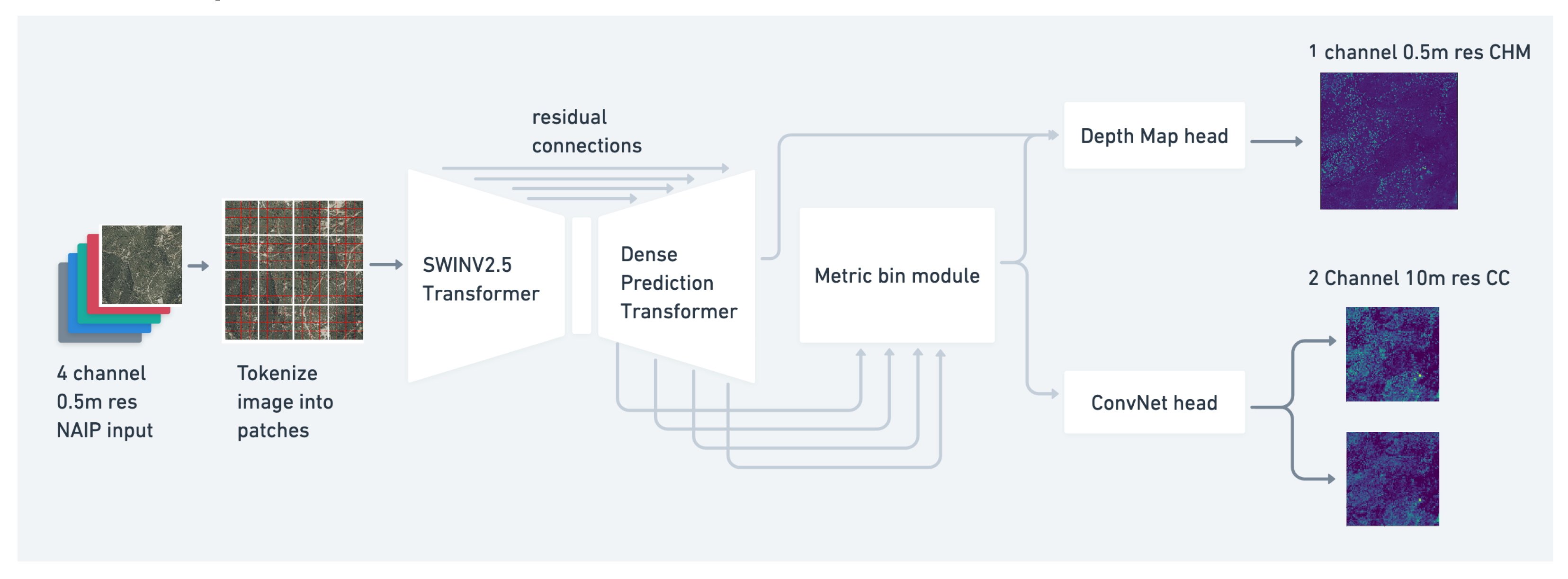
3.1. Vibrant Planet Multi-Task Vegetation Structure ViT: VibrantVS

We implemented the VibrantVS model using the PyTorch deep-learning framework [46], leveraging its efficient tensor operations, automatic differentiation, and GPU acceleration for large-scale model training. The VibrantVS model consists of three main components: a base model and two heads. The base model employs an encoder–decoder Vision Transformer (ViT) architecture, while the heads are a metric-bin module head [47] and a light-weight convolution head. The encoder is derived from a modified version of the SWINv2 model [48], while the decoder uses a dense prediction transformer (DPT) [49] (Figure 4). The DPT module processes features generated by the encoder to produce a normalized relative depth map. These features, along with dense features from the encoder via skip connections, are subsequently input into the metric-bin module head to predict canopy height and into the convolutional prediction head to predict canopy cover (CC).
The metric-bin module head learns the height distribution for each pixel, represented by 64 bins. These bins are linearly combined to generate dense features that are subsequently merged with feature tensors from the encoder through residual layers. The final output provides tree-height metrics at a resolution of 0.5 m and canopy cover at a resolution of 10 m. Note that although this model produces both CHM and CC, we only evaluated the CHM portion in this research.
VibrantVS uses a custom modified version of SWINv2 to incorporate the latest transformer-architecture advancements, including token registers, as described in [50]; this stabilized training and reduced noise in latent-attention features. Furthermore, we reconfigured the attention module to use grouped query attention [51], Flash Attention V2 [52], and SWIGLU [53] activation with RMSNORM [54]. These modifications result in reduced training time and improved model convergence stability.
Certain recent optimization techniques, such as schedule-free optimization [55], did not converge effectively. However, the 8-bit Adam optimizer [56] demonstrated satisfactory performance and accelerated training compared to the traditional float32-based AdamW optimizer.
We extended the inference context window from 384 × 384 pixels to 1536 × 1536 pixels, enabling the model to produce more consistent and artifact-free outputs when handling NAIP inputs of varying quality, including optical artifacts such as seam lines resulting from the merging of data from different flight paths.
The model was trained end to end in a multi-task learning setting to predict both canopy height and canopy cover. Empirical results indicated that L1 loss outperformed Sigloss, providing improved training stability while requiring fewer learnable hyperparameters. The model was trained using input NAIP tiles, paired with dense canopy height data at a 0.5 m resolution and canopy cover data at a 10 m resolution. The model training on this dataset, approximately 10 terabytes in size, took 2688 A100 GPU hours. Training was conducted for 318,528 steps, with a batch size of 16 per A100 node, using a learning rate of 4 × 10⁻⁵ and a one cycle learning rate scheduler [57].
The scheduler was configured by setting the initial learning rate equal to the maximum learning rate of 4 × 10⁻⁵ and a division factor of 1000, thereby reducing the learning rate to 1/1000 of its peak value by the end of training. A warm-up phase was implemented, during which, on 30% of the training batches, the learning rate was gradually increased to the maximum learning rate before decay commenced. The decay followed a single-cycle schedule with a polynomial annealing exponent of 1.0 [57].
Momentum was adjusted cyclically, ranging from a base momentum of 0.85 to a maximum of 0.95, to facilitate adaptive optimization. This configuration stabilized training, mitigated oscillations, and led to faster convergence by improving the efficiency of the optimization process [58].
To mitigate tiling checkerboard artifacts during inference, the PyTorch functions ‘fold’ and ‘unfold’ were replaced with an in-memory buffer cache that makes use of memory pointers. This optimization facilitates the seamless merging of multiple inferences across tiles much larger than the model’s context window, enabling inference over regions up to 100,000 × 100,000 pixels using a single Nvidia 24 GB A10G GPU.
We summarize VibrantVS and the baseline models (Meta, LANDFIRE, and ETH) in Table A1.

3.2. Calculating Error Metrics

We applied a number of error metrics to all baseline models to evaluate the performance of the CHMs that include mean absolute error (MAE), coefficient of determination (R²), Block-R2, root mean squared error (RMSE), mean absolute percent error (MAPE), mean error (ME), and edge error metric (EE) (see Appendix for error metric equations). These metrics were applied to VibrantVS and the baseline models after masking lidar CHM pixels < 2 m in order to only include pixels that had a high potential to represent trees or higher vegetation. This reduced noise from low-lying vegetation or surface features, which were not relevant for our canopy height study [59]. We also masked out lidar pixels where there were no data due to incomplete test tiles that may border flight path edges. To apply our error metrics, we spatially intersected all lidar CHM test tiles (500 × 500 m2 area; 1000 × 1000 pixels at 0.5 m spatial resolution) with VibrantVS and the baseline model CHMs. We then calculated the pixel-wise error metric across all 1,000,000 pixels in the test tile, accounting for all masked pixels. We repeated this for all test tiles and took the median error metric across tiles aggregated by the following:
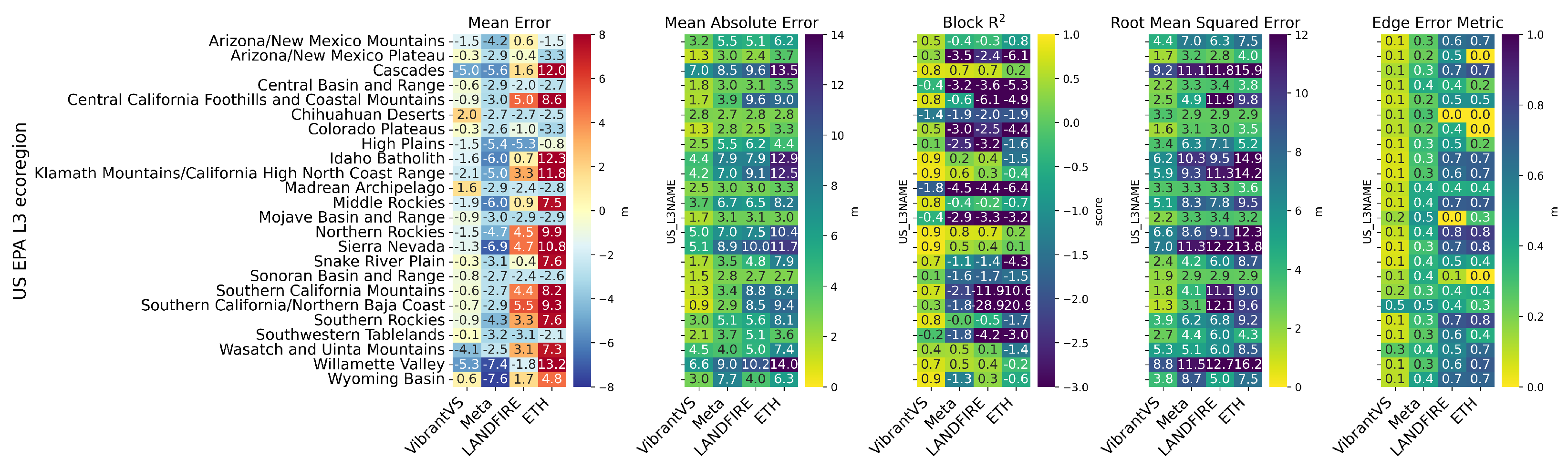
  • The majority spatial intersection of tiles with the corresponding EPA L3 ecoregion to determine ecoregion-level accuracies.
  • Individual height bins within each tile to determine height-class accuracies.

4. Results

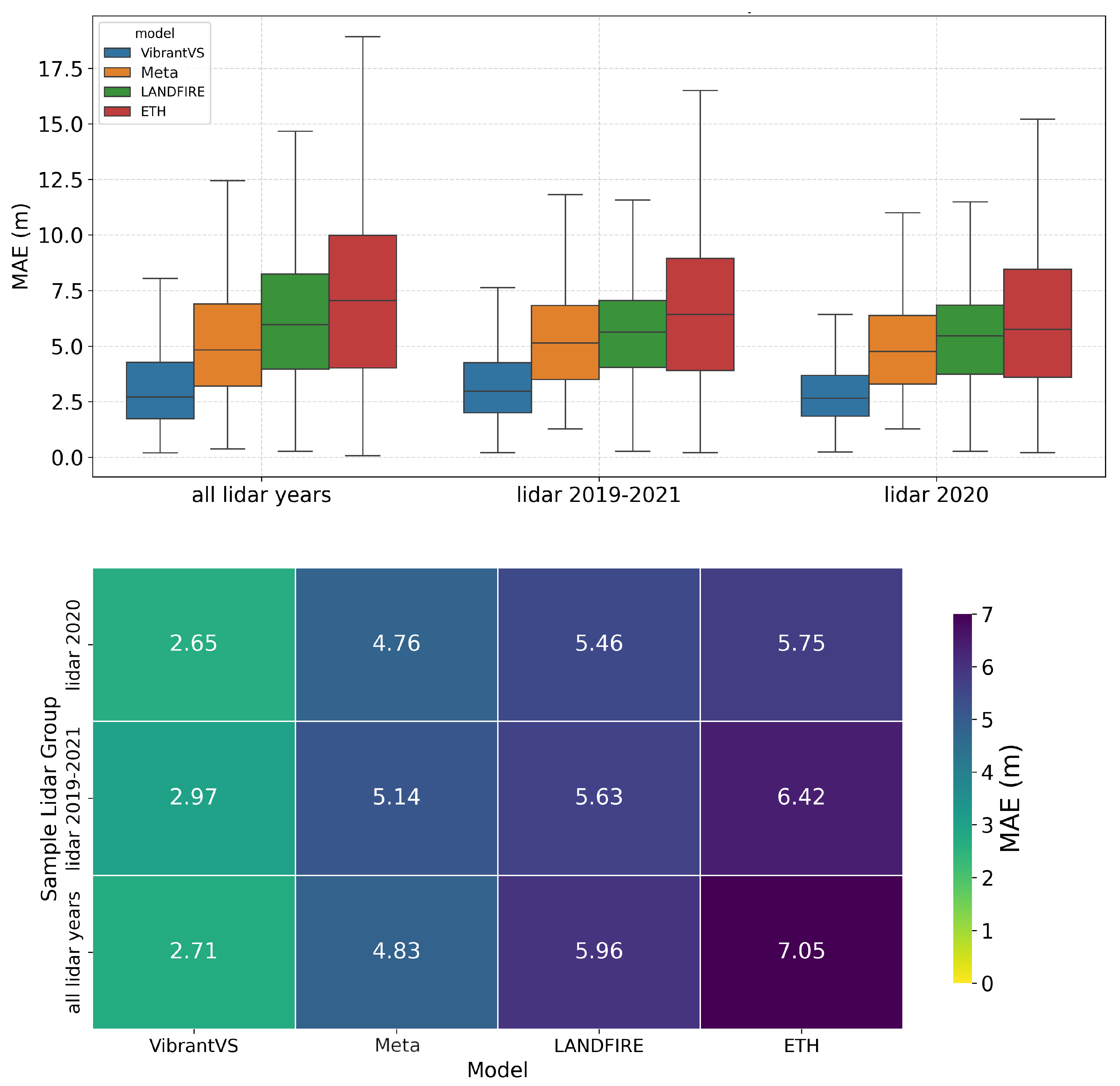
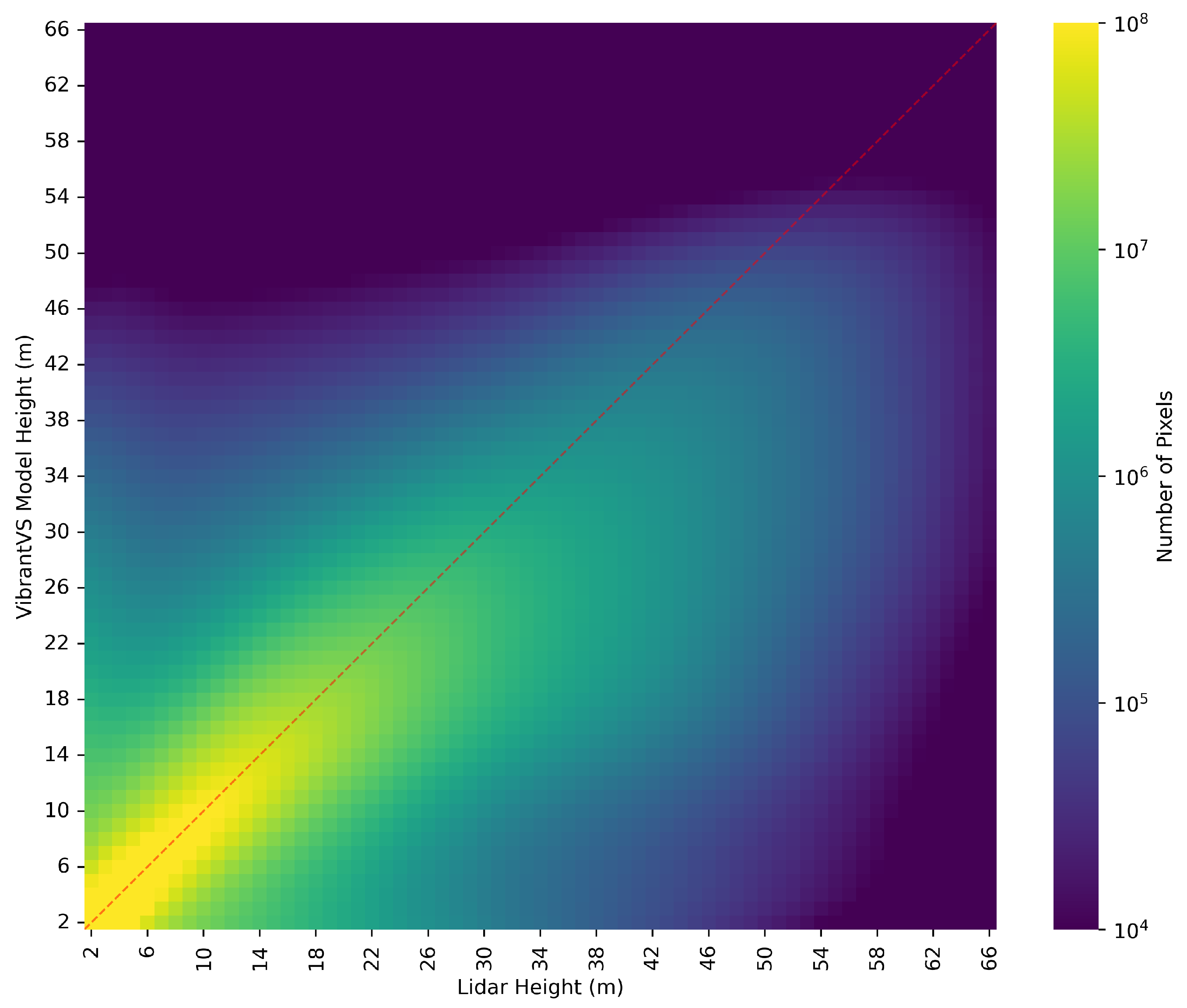
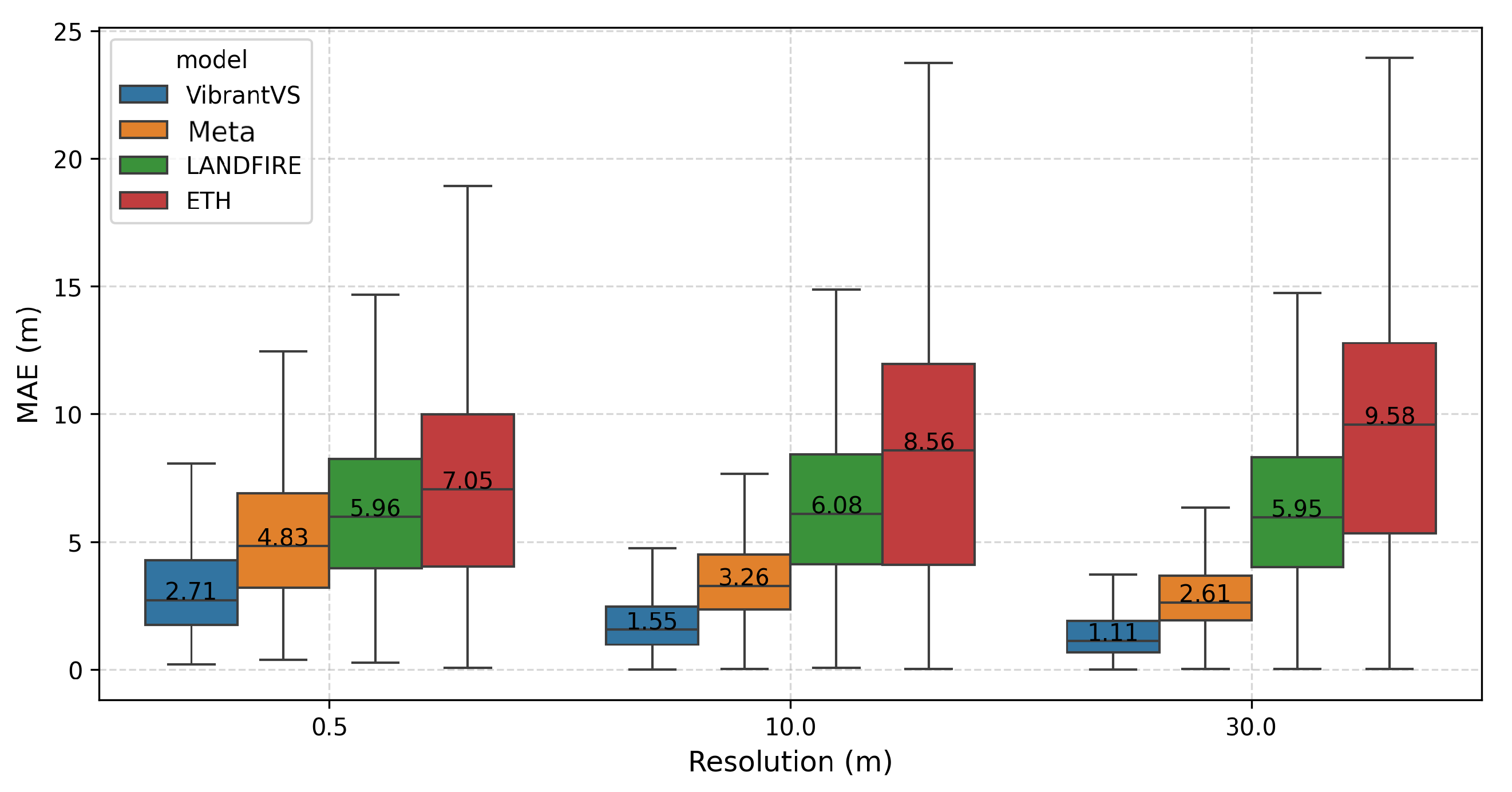
4.1. Overall Model Performance

VibrantVS outperforms all baseline models, with an overall median MAE of 2.71 m, Meta: 4.83 m; LANDFIRE: 5.96 m; and ETH: 7.05 m (Table 2). The overall mean error results show a median underestimation of canopy heights of 1.11 m by VibrantVS, 4.03 m by Meta, and a median overestimation by LANDFIRE of 0.92 m and by the ETH model of 5.65 m (Table 2).
The summaries in Table 2 indicate that VibrantVS outperforms the other baseline models for mean absolute error (MAE), Block-R2, and edge error metrics, suggesting a better ability to synthesize lidar-like CHM outputs. The median Block-R2 [25] numbers across all tiles also reflect the performance trend of MAE and ME (compare Table 2).

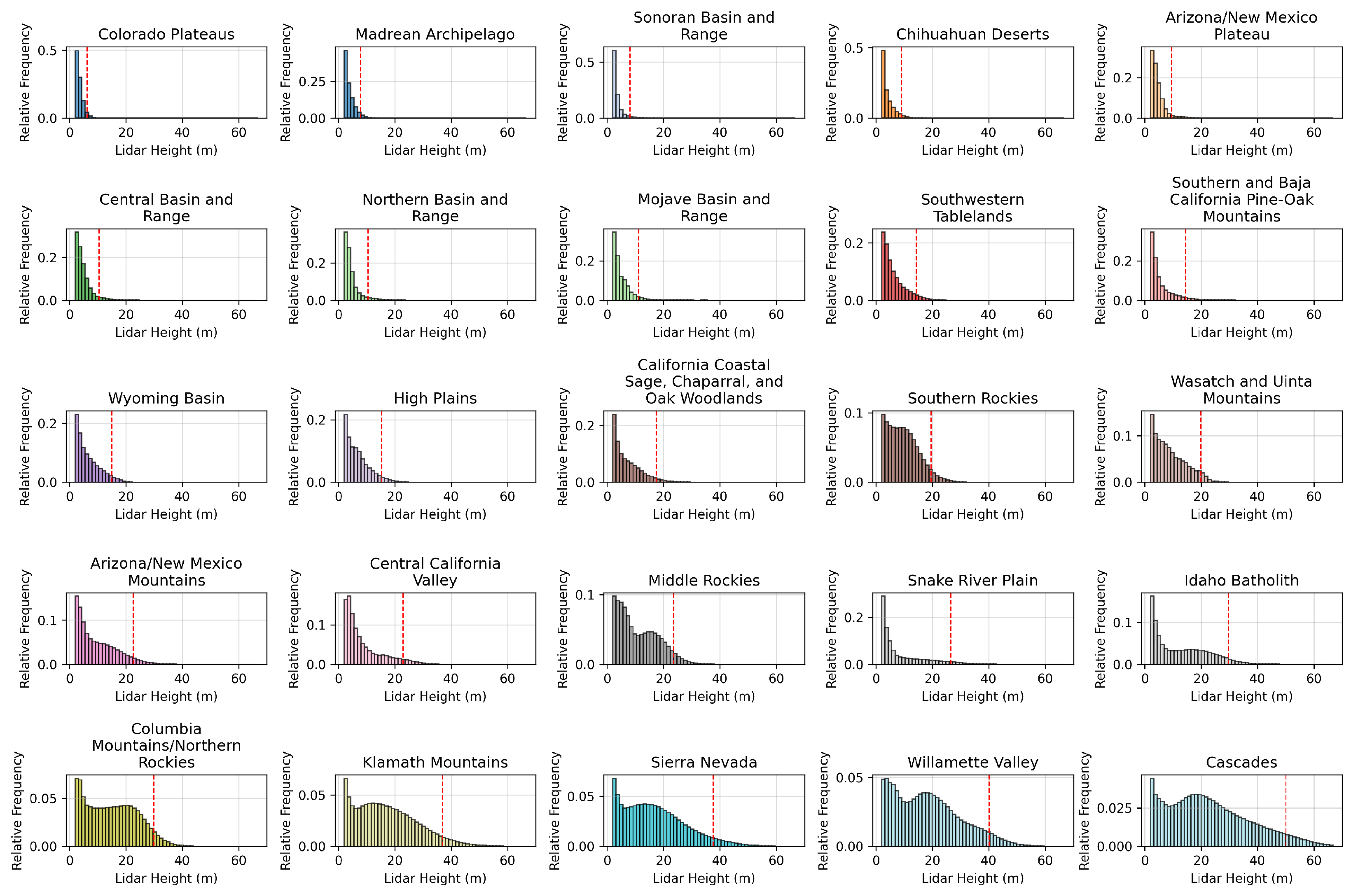
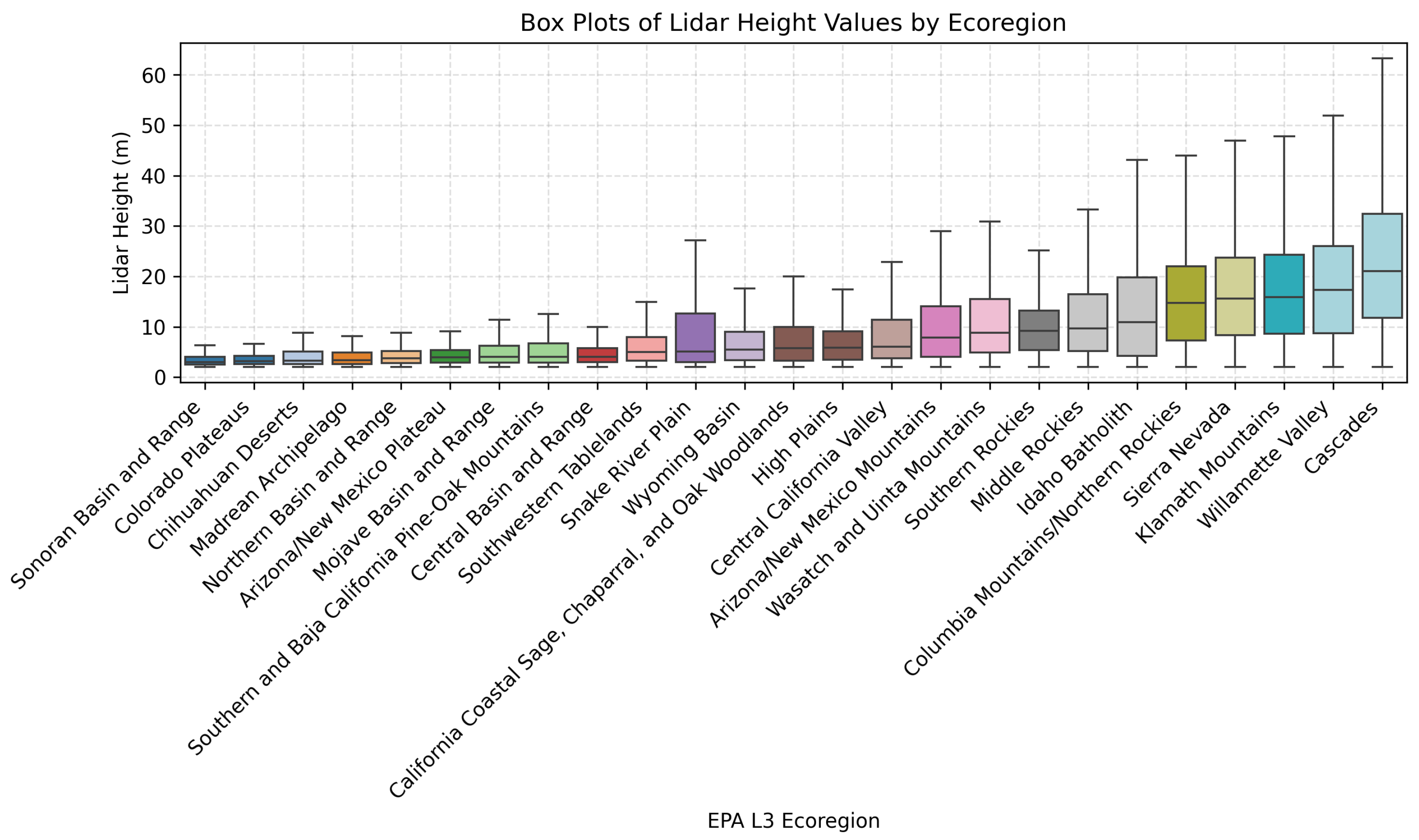
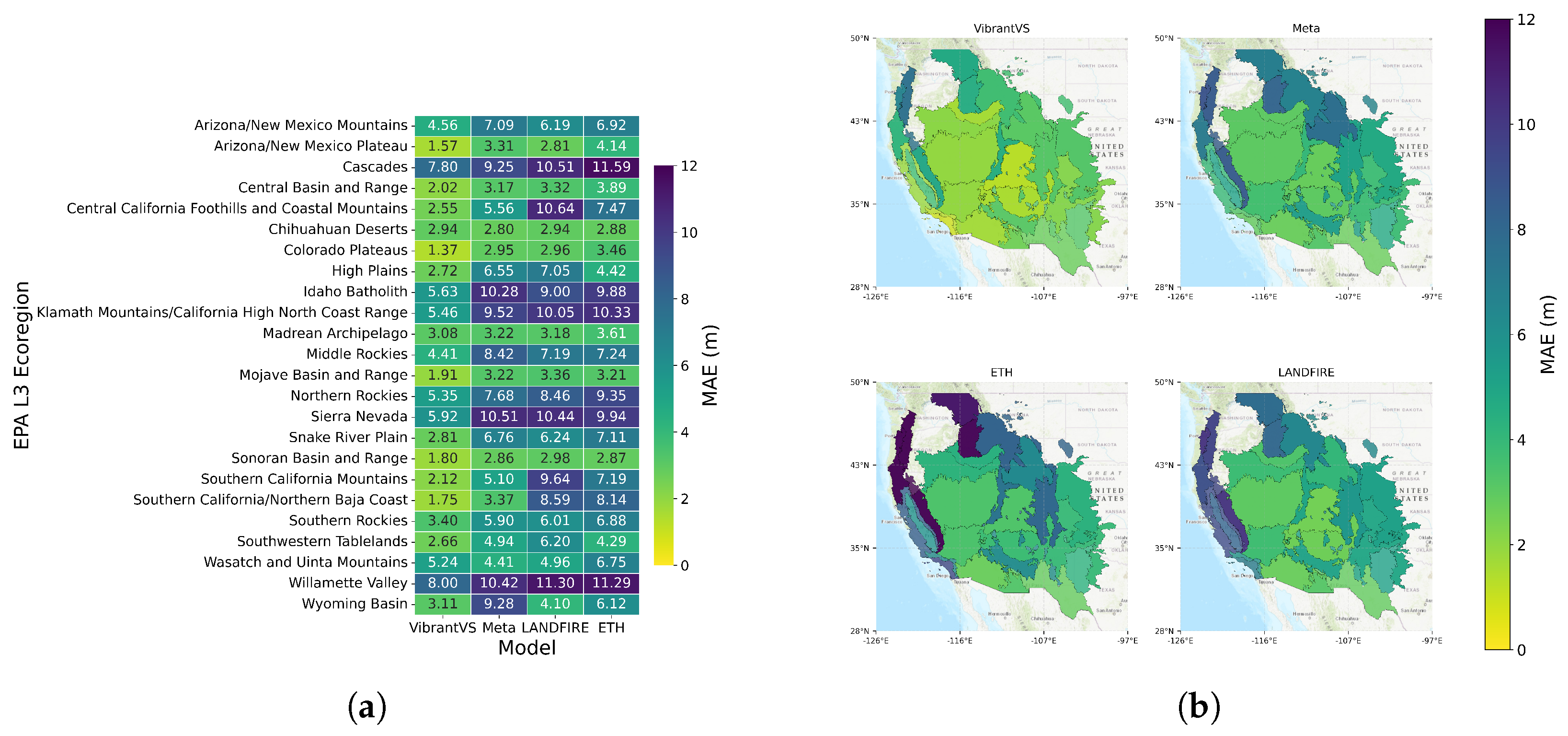
4.2. Performance Across Ecoregions

The VibrantVS model consistently demonstrates lower error ranges in nearly all ecoregions analyzed, as evidenced by the narrower box plot widths for MAE for this model (Figure 5). This highlights the higher CHM accuracy of VibrantVS at the tile level.
The observed error of VibrantVS is consistently the lowest in desert and low-elevation ecoregions, where vegetation heights are typically below 10 m in height, demonstrating high accuracy in shrub and grass systems. As shown in Figure 6, the error increases substantially in western forests, where the 95th percentile of lidar heights is above 25 m, suggesting that taller long-lived trees such as coastal redwoods and cedars pose a substantial challenge for all baseline models and the VibrantVS model (Figure 5 and Figure 6). This is reflected in the MAE map (Figure 7b), where MAE increases within ecoregions where there are larger species of western trees (see Figure A2 for lidar canopy height box plots by ecoregion). VibrantVS’s largest MAE values occur in the Cascades and Willamette Valley ecoregions, in which the other models also tend to perform worst (Figure 5).
The observed error of VibrantVS is consistently the lowest in desert and low-elevation ecoregions, where vegetation heights are typically below 10 m, demonstrating high accuracy in shrub and grassland systems. However, as shown in Figure 6, errors increase substantially in dense western forests, where the 95th percentile of lidar heights exceeds 25 m. This suggests that taller, long-lived tree species such as coastal redwoods and cedars pose a substantial challenge for all baseline models, including VibrantVS (Figure 5 and Figure 6).

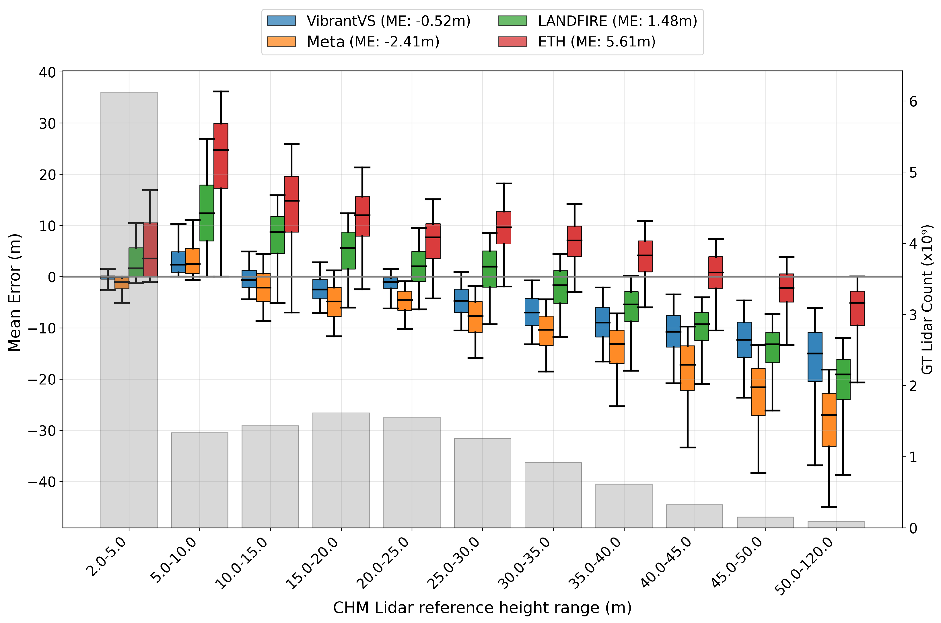
4.3. Performance Across Binned Tree Heights

Our evaluation shows that all four models tend to truncate tree heights above 50 m, with ETH’s model performing best in this height range (Figure 6 and Figure 8).
The mean-error results by canopy height bins show that VibrantVS has less bias than the other baseline models in the range of 2 to 25 m. These height classes coincide with the majority of the lidar pixels in our test data. Beyond these heights, LANDFIRE and ETH tend to outperform VibrantVS when compared to lidar (Figure 9). However, while the VibrantVS and Meta models tend to show increasingly negative mean errors at higher height bins, both LANDFIRE and ETH strongly overestimate lower canopy height bins.
Figure 8 shows the complete 2D histogram of the range of VibrantVS’s predicted tree heights versus lidar-based tree heights.

4.4. Qualitative Analysis

The Meta and VibrantVS CHM estimates provide finer resolution data that are visually closer to the corresponding aerial lidar data, resulting in higher fidelity for fine-scale applications (Figure 10). This is made evident by the lower median edge errors (EEs) observed for these models compared to ETH and LANDFIRE (see Appendix A, Equation (A5)) between the models, where VibrantVS’s EE equals 0.08, compared to Meta with 0.3, and ETH and LANDFIRE at 0.63 and 0.64 (Table 2, Figure 11). Considering the coarser resolution of the LANDFIRE and ETH data, their estimates often result in a constant value and a general overestimation of the CHM values compared to lidar and a lower underestimation in canopy heights beyond 30 m (Figure 6). When we aggregate VibrantVS’s results to 10 m and 30 m and compare them with the baseline models at the same resolution, we find that the trends in differences between the overall median MAEs are consistent with the 0.5 m results. At 10 m resolution, VibrantVS’s median MAE is the lowest, with 1.55, compared to a median MAE of 3.26 and above for the baseline models. At 30 m resolution, VibrantVS has a median MAE of 1.11, compared to 2.61 and higher values of the baseline models (Figure 12).

5. Discussion

In this paper, we evaluate a novel vision transformer model against other baseline canopy height models. Our results demonstrate that the VibrantVS model produces a high-accuracy, high-precision CHM across ecoregions in the western United States.
The overall performance of the VibrantVS model is likely better than the baseline models because we use a larger quantity of training data from a broader set of ecoregions (Table 1, Figure 3). Our training and test data are based on a canopy height model created from aerial lidar from a wide range of ecoregions in the western United States, with a total surface area of about 190,000 km2, allowing our model to learn a wider range of landscape canopy-height patterns. In contrast, the baseline models were trained on more limited regions: NEON sites, Forest Inventory and Analysis (FIA) field plots, or select GEDI plots, that may represent sets of conditions that are too limited to create a robust model. Although other factors such as the use of higher resolution NAIP imagery have contributed as well, we attribute most of our performance gains to our robust training dataset and especially to our selection of model improvements for our ViT. Wagner et al. [24] used a U-Net-based approach with the same type of NAIP input data to estimate canopy heights, but evaluated the performance only in California, and therefore we could not include them in this analysis.
The temporal alignment of our NAIP images is within a single year of the acquisition date of the aerial lidar for the data used to train VibrantVS. However, this is not the case for the other baseline models. They all aim to represent a CHM from the year 2020; however, their source data come from a wider range of acquisition years: Maxar mosaic data from 2018 to 2022 [25], Landsat data from 2016 [44], or Sentinel-2-L2A data from 2020 [26]. The temporal discrepancy with the acquisition years from 2016 to 2021 of the aerial lidar led to larger estimation errors. However, even when we only compare the models with corresponding lidar data from 2019 to 2021, the trend in the difference in MAE numbers is maintained (Figure A3). This highlights a specific advantage of the use of NAIP imagery as a model input, given NAIP’s three-year-or-less temporal return interval. This cadence across states allows for the monitoring of canopy heights following major disturbances and can provide updated information of the forest structure without the cost of lidar acquisition.
VibrantVS utilizes higher resolution source image data from NAIP compared to the other models. A resolution of 0.5 m provides better granularity of the features within the image and allows us to provide native estimates at 0.5 m, which aligns with the aerial lidar CHM that we compare against. Meta provides a CHM at 1 m resolution, ETH at 10 m, and LANDFIRE at 30 m. Given our use of nearest-neighbor resampling to compare our baselines versus lidar, we expected high-resolution comparisons to inflate MAE for baseline models due to their lower native resolutions compared to VibrantVS, but this is not the case when observing MAE for aggregations at spatial resolutions at 10 m and 30 m. When we compare all models at 10 m and 30 m resolutions to the lidar CHM at these same resolutions, the trend in differences of overall median MAE is maintained relative to the 0.5 m results (Figure 12).
The coarser resolution of the ETH and LANDFIRE models restricts their use to coarse-level applications, for which the trends in overestimation and underestimation at different tree heights could be accounted for with correction factors by height bins. The high resolution of the VibrantVS model provides the opportunity to generate downstream forest structure products such as Tree Approximate Object (TAO) segmentation [60]. The spatial resolution of a CHM is a critical factor in accurately segmenting individual trees, which often serve as inputs for various forest management activities. Higher resolutions, such as 0.5 m, can provide detailed canopy representations that a 1 m pixel resolution model might not capture, leading to less precise segmentation [61]. Furthermore, CHM rasters can serve as input to wildfire spread models, allowing practitioners to better capture discontinuities in fuels that may slow or stop fire progression [62].
All models tend to perform worse in high-altitude areas and areas with steep slopes (Figure 5 and Figure 7), for example, in the Cascades ecoregion. In VibrantVS’s case, this could be caused by an imbalance in training data, as the map of the location of training and test samples shows (Figure 1). For example, in high-altitude areas from which more training data were sampled, the performance of VibrantVS is better: the median MAE in the Klamath Mountains and Sierra Nevada ecoregions is lower than the MAE of the Cascades (Figure 5).
The underestimation of heights in very tall trees is likely caused by an imbalance in our training data, as such trees constitute a low percentage of the total number of trees and occur only in a few ecoregions.
The training and test data used in this study cover only a small fraction of the total area of the western United States and its variety of environmental and ecological conditions. However, even in ecoregions with little or no training data, the model performs as good or better than the baseline models, but performs worse there than in ecoregions with more training data (compare Figure 3 and Figure 5).
From our analysis, we determine that the following improvements can be made in future research:
  • More refinements can be made to the evaluations of the lowest height bin. MAE values are higher in this category because the spatial footprint of tree crowns appear larger in NAIP data compared to lidar-based tree crowns. This aerial image-based effect causes the VibrantVS model to infer a wider canopy crown that results in an overestimation of values where the lidar data are closer to 0. If we use the block metrics of Tolan et al. [25], rather than the pixel-wise metrics of Lang et al. [26], then we expect the lowest bin error of overestimation to disappear.
  • More importantly, we have to address the underestimation of height among trees that are taller than 35 m, and especially trees taller than 50 m. There is an imbalance in the number of training samples of tall trees. Trees taller than 50 m represent less than 0.5% of our training data. We are undertaking a specific retraining exercise to address this underestimation and to compensate for the label imbalance.
  • We would like to integrate topography data into our model, as we suspect that this could improve accuracy, especially on steep slopes and in high-altitude regions.
  • We are also planning to expand our range of applications to more ecoregions, especially in the central and eastern United States. This would allow us to include additional tree species and also shrub vegetation types and to evaluate CHMs at heights lower than 2 m.

6. Conclusions

This paper presents a comprehensive analysis of three baseline CHM models and our custom vision transformer model (VibrantVS), which is based on NAIP imagery. Our findings indicate that, while each model has its strengths, their success varies significantly between different ecoregions. VibrantVS outperforms all three baseline models in both accuracy and precision across the majority of ecoregions and ranges of canopy heights. It comes with the distinct advantage of being able to produce a very high resolution (0.5 m) CHM and can be updated with a cadence of three years or less. Furthermore, VibrantVS is based on publicly and freely available data in the United States and can be an alternative to collecting aerial lidar at high costs to monitor forests.
The very high resolution CHMs from VibrantVS can be used in the TAO segmentation process, which allows for the downstream estimation of key forest-structure variables, such as trees per acre, basal area, timber volume, canopy base height, and biomass. These variables are essential for decision-making in forestry and land management and are also key to planning in many conservation efforts. These derived variables can also be integrated into existing fire models to predict fire risk and behavior at high resolution.
Future research will expand the training and application of VibrantVS to areas in the central and eastern United States, as well as internationally.

Author Contributions

Conceptualization, T.C., K.N. and S.C.; methodology, K.N. and A.G.; software, K.N., V.A.L. and B.S.; validation, T.C., K.N. and L.J.Z.; formal analysis, T.C. and K.N.; investigation, K.N. and V.A.L.; resources, B.S. and M.A.G.; data curation, V.A.L., L.J.Z. and M.A.G.; writing—original draft preparation, T.C., K.N., A.G. and C.W.M.; writing—review and editing, T.C., A.G., V.A.L., L.J.Z. and N.E.R.; visualization, T.C. and K.N.; supervision, T.C., A.G., N.E.R. and G.B.; project administration, T.C., N.E.R. and G.B.; funding acquisition, T.C. and S.C. All authors have read and agreed to the published version of the manuscript.

Funding

This research was funded by the United States Department of Agriculture, grant number NR233A750004G042, and the National Aeronautics and Space Administration, grant number 80NSSC22K1734.

Data Availability Statement

The model test data can be found here: https://osf.io/kh4x3.

Acknowledgments

The authors would like to thank Leo Tsourides and Derek Young for their support and consulting in this research. Additional gratitude is extended to Ian Reese, Fabian Döweler, Finlay Thompson, and the rest of the Dragonfly Data Science team for initial proof-of-concept work. The authors thank NASA and USDA for their support.

Conflicts of Interest

Tony Chang, Kiarie Ndegwa, Andreas Gros, Vincent A. Landau, Luke J. Zachmann, Bogdan State, Mitchell A. Gritts, Colton W. Miller, Nathan E. Rutenbeck, Scott Conway, and Guy Bayes are employed by the company Vibrant Planet PBC. The grant funders had no role in the design of the study; in the collection, analyses, or interpretation of data; in the writing of the manuscript; or in the decision to publish the results.

Abbreviations

The following abbreviations are used in this manuscript:
3DEP3D Elevation Program
AWS S3Amazon Web Services Simple Storage Service
CCCanopy Cover
CHMCanopy Height Model
DEMDigital Elevation Model
DINOv2       Self DIstillation With NO Labels
DPTDense Prediction Transformer
DSMDigital Surface Model
DTMDigital Terrain Model
EEEdge Error
EPAEnvironmental Protection Agency
ETHEidgenössische Technische Hochschule Zürich
FCHForest Canopy Height
FIAForest Inventory and Analysis
GEDIGlobal Ecosystem Dynamics Investigation
GPUGraphics Processing Unit
LANDFIRELandscape Fire and Resource Management Planning Tools
L3Level 3 Ecoregion
MAEMean Absolute Error
MEMean Error
NAIPNational Agriculture Inventory Program
NEONNational Ecological Observatory Network
RMSERoot Mean Squared Error
RMSNORMRoot Mean Square Layer Normalization
SWIGLUSwish Gated Linear Unit
SWINv2Shifted Window
TAOTree Approximate Object
TIFFTagged Image File Format
USFSUnited States Forest Service
USGSUnited States Geological Survey
ViTVision Transformer
WCSWildfire Crisis Strategy
WESMWork Unit Extent Spatial Metadata

Appendix A

Appendix A.1. Additional Tables and Figures

Figure A1. Lidar sample pixel-wise height distributions within each of the EPA Level 3 ecoregions. Red dashed line represents the 95th percentile of the height distribution.
Remotesensing 17 01017 g0a1
Figure A2. Lidar sample tile height box plots within each EPA Level 3 ecoregion.
Remotesensing 17 01017 g0a2
Figure A3. Comparison of model performance at different year groups of lidar acquisition determine temporal mismatch error.
Remotesensing 17 01017 g0a3
Table A1. Summary of CHM models, spatial resolutions, predictor data, and label data.
ModelSpatial ResolutionSpatial ExtentTemporal CoverageArchitecturePredictor DataLabel Data
VibrantVS0.5 mWestern United States2014–2021Multi-task vision transformer4-band NAIP imageryUSGS 3DEP aerial lidar
Meta [25]1 mGlobal2020Encoder, dense prediction transformer, correction and rescaling networkMaxar Vivid2 0.5 m resolution mosaicsNEON aerial lidar CHMs, GEDI data, and a labeled 9000 tile tree/no tree segmentation dataset
LANDFIRE [43]30 mUnited States2016, 2020, 2022, 2023Regression-tree based methodsSpectral information from Landsat, landscape features such as topography, and biophysical informationField-measured height
ETH [26]10 mGlobal2020Deep learning ensembleSentinel-2-L2A multi-spectral imagery, sin-cos embeddings of longitudinal coordinatesSparse GEDI lidar data

Appendix A.2. Error Metrics

  • Mean Absolute Error (MAE)
    MAE = 1 n i = 1 n y i y ^ i
  • Block-R2
    R block 2 = 1 b = 1 B i b ( y i y ^ i ) 2 b = 1 B i b ( y i y ¯ b ) 2
    where B is the number of blocks, y b is the ground truth value in block b, y ^ b is the model estimate for block b, and y ¯ b is the mean of the ground-truth values in block b.
  • Root Mean Square Error (RMSE)
    RMSE = 1 n i = 1 n y i y ^ i 2
  • Mean Error (ME)
    ME = 1 n i = 1 n y ^ i y i
  • Edge Error Metric (EE)
    EE = 1 n i = 1 n E ( y ^ i ) E ( y i )
    where E ( · ) represents Sobel edge detection operation on the data (also compare Tolan et al. [25]).

References

  1. Moritz, M.A.; Batllori, E.; Bradstock, R.A.; Gill, A.M.; Handmer, J.; Hessburg, P.F.; Leonard, J.; McCaffrey, S.; Odion, D.C.; Schoennagel, T.; et al. Learning to coexist with wildfire. Nature 2014, 515, 58–66. [Google Scholar] [CrossRef] [PubMed]
  2. Westerling, A.L. Increasing western US forest wildfire activity: Sensitivity to changes in the timing of spring. Philos. Trans. R. Soc. B Biol. Sci. 2016, 371, 20150178. [Google Scholar] [CrossRef] [PubMed]
  3. Abatzoglou, J.T.; Williams, A.P. Impact of anthropogenic climate change on wildfire across western US forests. Proc. Natl. Acad. Sci. USA 2016, 113, 11770–11775. [Google Scholar] [CrossRef]
  4. Stevens-Rumann, C.S.; Kemp, K.B.; Higuera, P.E.; Harvey, B.J.; Rother, M.T.; Donato, D.C.; Morgan, P.; Veblen, T.T. Evidence for declining forest resilience to wildfires under climate change. Ecol. Lett. 2018, 21, 243–252. [Google Scholar] [CrossRef] [PubMed]
  5. Hessburg, P.F.; Agee, J.K.; Franklin, J.F. Dry forests and wildland fires of the inland Northwest USA: Contrasting the landscape ecology of the pre-settlement and modern eras. For. Ecol. Manag. 2005, 211, 117–139. [Google Scholar] [CrossRef]
  6. Hoffman, K.M.; Davis, E.L.; Wickham, S.B.; Schang, K.; Johnson, A.; Larking, T.; Lauriault, P.N.; Quynh Le, N.; Swerdfager, E.; Trant, A.J. Conservation of Earth’s biodiversity is embedded in Indigenous fire stewardship. Proc. Natl. Acad. Sci. USA 2021, 118, e2105073118. [Google Scholar] [CrossRef]
  7. Van Leeuwen, M.; Nieuwenhuis, M. Retrieval of forest structural parameters using LiDAR remote sensing. Eur. J. For. Res. 2010, 129, 749–770. [Google Scholar] [CrossRef]
  8. Means, J.E.; Acker, S.A.; Harding, D.J.; Blair, J.B.; Lefsky, M.A.; Cohen, W.B.; Harmon, M.E.; McKee, W.A. Use of large-footprint scanning airborne lidar to estimate forest stand characteristics in the Western Cascades of Oregon. Remote Sens. Environ. 1999, 67, 298–308. [Google Scholar] [CrossRef]
  9. Riaño, D.; Meier, E.; Allgöwer, B.; Chuvieco, E.; Ustin, S.L. Modeling airborne laser scanning data for the spatial generation of critical forest parameters in fire behavior modeling. Remote Sens. Environ. 2003, 86, 177–186. [Google Scholar] [CrossRef]
  10. Andersen, H.E.; McGaughey, R.J.; Reutebuch, S.E. Estimating forest canopy fuel parameters using LIDAR data. Remote Sens. Environ. 2005, 94, 441–449. [Google Scholar] [CrossRef]
  11. Silva, C.A.; Hudak, A.T.; Vierling, L.A.; Loudermilk, E.L.; O’Brien, J.J.; Hiers, J.K.; Jack, S.B.; Gonzalez-Benecke, C.; Lee, H.; Falkowski, M.J.; et al. Imputation of individual longleaf pine (Pinus palustris Mill.) tree attributes from field and LiDAR data. Can. J. Remote Sens. 2016, 42, 554–573. [Google Scholar] [CrossRef]
  12. Popescu, S.C.; Wynne, R.H. Seeing the trees in the forest. Photogramm. Eng. Remote Sens. 2004, 70, 589–604. [Google Scholar] [CrossRef]
  13. Vierling, K.T.; Vierling, L.A.; Gould, W.A.; Martinuzzi, S.; Clawges, R.M. Lidar: Shedding new light on habitat characterization and modeling. Front. Ecol. Environ. 2008, 6, 90–98. [Google Scholar] [CrossRef]
  14. Lefsky, M.A.; Cohen, W.B.; Parker, G.G.; Harding, D.J. Lidar remote sensing for ecosystem studies. BioScience 2002, 52, 19–30. [Google Scholar] [CrossRef]
  15. Beland, M.; Parker, G.; Sparrow, B.; Harding, D.; Chasmer, L.; Phinn, S.; Antonarakis, A.; Strahler, A. On promoting the use of lidar systems in forest ecosystem research. For. Ecol. Manag. 2019, 450, 117484. [Google Scholar] [CrossRef]
  16. Wulder, M.A.; Bater, C.W.; Coops, N.C.; Hilker, T.; White, J.C. The role of LiDAR in sustainable forest management. For. Chron. 2008, 84, 807–826. [Google Scholar] [CrossRef]
  17. White, J.C.; Coops, N.C.; Wulder, M.A.; Vastaranta, M.; Hilker, T.; Tompalski, P. Remote sensing technologies for enhancing forest inventories: A review. Can. J. Remote Sens. 2016, 42, 619–641. [Google Scholar] [CrossRef]
  18. Olszewski, J.H.; Bailey, J.D. LiDAR as a Tool for Assessing Change in Vertical Fuel Continuity Following Restoration. Forests 2022, 13, 503. [Google Scholar] [CrossRef]
  19. Kramer, H.A.; Collins, B.M.; Kelly, M.; Stephens, S.L. Quantifying ladder fuels: A new approach using LiDAR. Forests 2014, 5, 1432–1453. [Google Scholar] [CrossRef]
  20. Franklin, S.E.; Lavigne, M.B.; Wulder, M.A.; Stenhouse, G.B. Change detection and landscape structure mapping using remote sensing. For. Chron. 2002, 78, 618–625. [Google Scholar] [CrossRef]
  21. Dubayah, R.O.; Drake, J.B. Lidar remote sensing for forestry. J. For. 2000, 98, 44–46. [Google Scholar] [CrossRef]
  22. Drusch, M.; Del Bello, U.; Carlier, S.; Colin, O.; Fernandez, V.; Gascon, F.; Hoersch, B.; Isola, C.; Laberinti, P.; Martimort, P.; et al. Sentinel-2: ESA’s optical high-resolution mission for GMES operational services. Remote Sens. Environ. 2012, 120, 25–36. [Google Scholar] [CrossRef]
  23. Valbuena, R.; O’Connor, B.; Zellweger, F.; Simonson, W.; Vihervaara, P.; Maltamo, M.; Silva, C.A.; Almeida, D.R.A.D.; Danks, F.; Morsdorf, F.; et al. Standardizing ecosystem morphological traits from 3D information sources. Trends Ecol. Evol. 2020, 35, 656–667. [Google Scholar] [CrossRef] [PubMed]
  24. Wagner, F.H.; Roberts, S.; Ritz, A.L.; Carter, G.; Dalagnol, R.; Favrichon, S.; Hirye, M.C.; Brandt, M.; Ciais, P.; Saatchi, S. Sub-meter tree height mapping of California using aerial images and LiDAR-informed U-Net model. Remote Sens. Environ. 2024, 305, 114099. [Google Scholar] [CrossRef]
  25. Tolan, J.; Yang, H.I.; Nosarzewski, B.; Couairon, G.; Vo, H.V.; Brandt, J.; Spore, J.; Majumdar, S.; Haziza, D.; Vamaraju, J.; et al. Very high resolution canopy height maps from RGB imagery using self-supervised vision transformer and convolutional decoder trained on aerial lidar. Remote Sens. Environ. 2024, 300, 113888. [Google Scholar] [CrossRef]
  26. Lang, N.; Jetz, W.; Schindler, K.; Wegner, J.D. A high-resolution canopy height model of the Earth. Nat. Ecol. Evol. 2023, 7, 1778–1789. [Google Scholar] [CrossRef]
  27. Li, S.; Brandt, M.; Fensholt, R.; Kariryaa, A.; Igel, C.; Gieseke, F.; Nord-Larsen, T.; Oehmcke, S.; Carlsen, A.H.; Junttila, S.; et al. Deep learning enables image-based tree counting, crown segmentation, and height prediction at national scale. PNAS Nexus 2023, 2, pgad076. [Google Scholar] [CrossRef]
  28. U.S. Forest Service. Initial Landscape Investments to Support the National Wildfire Crisis Strategy; U.S. Department of Agriculture: Washington, DC, USA, 2022.
  29. Thibault, K.M.; Laney, C.M.; Yule, K.M.; Franz, N.M.; Mabee, P.M. The US National Ecological Observatory Network and the Global Biodiversity Framework: National research infrastructure with a global reach. J. Ecol. Environ. 2023, 47, 21. [Google Scholar] [CrossRef]
  30. U.S. Geological Survey. WESM Data Dictionary. 2024. Available online: https://www.usgs.gov/ngp-standards-and-specifications/wesm-data-dictionary/ (accessed on 7 August 2024).
  31. Omernik, J.M.; Griffith, G.E. Ecoregions of the conterminous United States: Evolution of a hierarchical spatial framework. Environ. Manag. 2014, 54, 1249–1266. [Google Scholar] [CrossRef]
  32. Earth Resources Observation And Science (EROS) Center. National Agriculture Imagery Program (NAIP); Earth Resources Observation and Science (EROS) Center: Sioux Falls, SD, USA, 2017. [CrossRef]
  33. AWS Open Data Registry. NAIP: National Agriculture Imagery Program. 2024. Available online: https://registry.opendata.aws/naip/ (accessed on 26 September 2024).
  34. Sugarbaker, L.J.; Constance, E.W.; Heidemann, H.K.; Jason, A.L.; Lukas, V.; Saghy, D.L.; Stoker, J.M. The 3D Elevation Program Initiative: A Call for Action; Technical report; U.S. Geological Survey: Reston, VA, USA, 2014.
  35. Roussel, J.R.; Auty, D.; Coops, N.C.; Tompalski, P.; Goodbody, T.R.; Meador, A.S.; Bourdon, J.F.; de Boissieu, F.; Achim, A. lidR: An R package for analysis of Airborne Laser Scanning (ALS) data. Remote Sens. Environ. 2020, 251, 112061. [Google Scholar] [CrossRef]
  36. Maxar Technologies. Maxar Vivid2 Mosaic Imagery Data. 2024. Available online: https://developers.maxar.com/docs/streaming-basemap (accessed on 8 August 2024).
  37. Dubayah, R.; Armston, J.; Healey, S.P.; Bruening, J.M.; Patterson, P.L.; Kellner, J.R.; Duncanson, L.; Saarela, S.; Ståhl, G.; Yang, Z.; et al. GEDI launches a new era of biomass inference from space. Environ. Res. Lett. 2022, 17, 095001. [Google Scholar] [CrossRef]
  38. Meta; World Resources Institute (WRI). High Resolution Canopy Height Maps (CHM). 2024. Available online: https://registry.opendata.aws/dataforgood-fb-forests (accessed on 27 September 2024).
  39. Rollins, M.G.; Keane, R.E.; Zhu, Z.; Menakis, J.P. An overview of the LANDFIRE prototype project. In The LANDFIRE Prototype Project: Nationally Consistent and Locally Relevant Geospatial Data for Wildland Fire Management Gen. Tech. Rep. RMRS-GTR-175; Rollins, M.G., Frame, C.K., Eds.; US Department of Agriculture, Forest Service, Rocky Mountain Research Station: Fort Collins, CO, USA, 2006; Volume 175, pp. 5–43. [Google Scholar]
  40. Watts, K.F.; Koehler, D.W.; Todd, D.; Gillett, N. Integration of LANDFIRE Data into Fire Modeling: Enhancing Accuracy and Consistency. J. Appl. Meteorol. Climatol. 2017, 56, 2017JA024010. [Google Scholar] [CrossRef]
  41. Steenburgh, S.L.; Schmid, K.R. LANDFIRE Program: Fuel Data for Fire and Resource Management Planning. Fire Ecol. 2012, 8, 89–96. [Google Scholar]
  42. Lane, M.L.; Swetnam, T.W.; Oki, T. Fuel Models and LANDFIRE: Standardizing Inputs for Fire Simulation. Int. J. Wildland Fire 2011, 20, 845–856. [Google Scholar]
  43. Rollins, M.G. LANDFIRE: A nationally consistent vegetation, wildland fire, and fuel assessment. Int. J. Wildland Fire 2009, 18, 235–249. [Google Scholar] [CrossRef]
  44. U.S. Geological Survey. LANDFIRE Fuels—Forest Canopy Height. 2022. Available online: https://www.landfire.gov/fuel/ch (accessed on 27 April 2024).
  45. ETH Zurich. Global Canopy Height Map for the Year 2020 Derived from Sentinel-2 and GEDI (Version 1); ETH Zurich Research Collection: Zurich, Switzerland, 2023. [Google Scholar] [CrossRef]
  46. Paszke, A.; Gross, S.; Massa, F.; Lerer, A.; Bradbury, J.; Chanan, G.; Killeen, T.; Lin, Z.; Gimelshein, N.; Antiga, L.; et al. PyTorch: An Imperative Style, High-Performance Deep Learning Library. In Proceedings of the Advances in Neural Information Processing Systems 32, San Diego, CA, USA, 8–14 December 2019; Wallach, H., Larochelle, H., Beygelzimer, A., d’Alché Buc, F., Fox, E., Garnett, R., Eds.; Curran Associates, Inc.: New York, NY, USA, 2019; Volume 32, pp. 8024–8035. [Google Scholar]
  47. Bhat, S.F.; Birkl, R.; Wofk, D.; Wonka, P.; Müller, M. Zoedepth: Zero-shot transfer by combining relative and metric depth. arXiv 2023, arXiv:2302.12288. [Google Scholar]
  48. Liu, Z.; Hu, H.; Lin, Y.; Yao, Z.; Xie, Z.; Wei, Y.; Ning, J.; Cao, Y.; Zhang, Z.; Dong, L.; et al. Swin transformer v2: Scaling up capacity and resolution. In Proceedings of the IEEE/CVF Conference on Computer Vision and Pattern Recognition, New Orleans, LA, USA, 18–24 June 2022; pp. 12009–12019. [Google Scholar]
  49. Ranftl, R.; Lasinger, K.; Hafner, D.; Schindler, K.; Koltun, V. Towards robust monocular depth estimation: Mixing datasets for zero-shot cross-dataset transfer. IEEE Trans. Pattern Anal. Mach. Intell. 2020, 44, 1623–1637. [Google Scholar] [CrossRef]
  50. Darcet, T.; Oquab, M.; Mairal, J.; Bojanowski, P. Vision transformers need registers. arXiv 2023, arXiv:2309.16588. [Google Scholar]
  51. Ainslie, J.; Lee-Thorp, J.; de Jong, M.; Zemlyanskiy, Y.; Lebrón, F.; Sanghai, S. Gqa: Training generalized multi-query transformer models from multi-head checkpoints. arXiv 2023, arXiv:2305.13245. [Google Scholar]
  52. Dao, T. Flashattention-2: Faster attention with better parallelism and work partitioning. arXiv 2023, arXiv:2307.08691. [Google Scholar]
  53. Shazeer, N. Glu variants improve transformer. arXiv 2020, arXiv:2002.05202. [Google Scholar]
  54. Zhang, B.; Sennrich, R. Root mean square layer normalization. In Proceedings of the NeurIPS Conference on Advances in Neural Information Processing Systems 32, Vancouver, CA, USA, 8–14 December 2019; pp. 12381–12392. [Google Scholar]
  55. Defazio, A.; Mehta, H.; Mishchenko, K.; Khaled, A.; Cutkosky, A. The Road Less Scheduled. arXiv 2024, arXiv:2405.15682. [Google Scholar]
  56. Dettmers, T.; Lewis, M.; Shleifer, S.; Zettlemoyer, L. 8-bit Optimizers via Block-wise Quantization. arXiv 2021, arXiv:abs/2110.02861. [Google Scholar]
  57. Smith, L.N. A Disciplined Approach to Neural Network Hyper-Parameters: Part 1—Learning Rate, Batch Size, Momentum, and Weight Decay. arXiv 2018, arXiv:1803.09820. [Google Scholar]
  58. Rumelhart, D.E.; Hinton, G.E.; Williams, R.J. Learning Representations by Back-Propagating Errors. Nature 1986, 323, 533–536. [Google Scholar] [CrossRef]
  59. Ferraz, A.; Bretar, F.; Jacquemoud, S.; Gonçalves, G.; Pereira, L.; Tomé, M.; Soares, P. 3D mapping of a multi-layered Mediterranean forest using ALS data. Remote Sens. Environ. 2012, 121, 210–223. [Google Scholar] [CrossRef]
  60. Jeronimo, S.M.A.; Kane, V.R.; Churchill, D.J.; McGaughey, R.J.; Franklin, J.F. Applying LiDAR Individual Tree Detection to Management of Structurally Diverse Forest Landscapes. J. For. 2018, 116, 336–346. [Google Scholar] [CrossRef]
  61. Team, R.L. LiDAR Data Analysis with R: Canopy Height Models. 2024. Available online: https://r-lidar.github.io/lidRbook/dsm.html?utm_source=chatgpt.com (accessed on 3 December 2024).
  62. Ritu, T.; James, H.; ad Reinke Karin, W.L.; Simon, J. Effect of fuel spatial resolution on predictive wildfire models. Int. J. Wildland Fire 2021, 30, 776–789. [Google Scholar] [CrossRef]
Figure 2. Map of EPA L3 ecoregions into which our test tiles were aggregated to evaluate baseline model performance.
Remotesensing 17 01017 g002
Figure 3. Sample tile counts within each of the randomly sampled training and test (approx. 85% to 15% ratio) groups by EPA L3 ecoregion.
Remotesensing 17 01017 g003
Figure 4. VibrantVS multi-task vision transformer architecture with 4-band NAIP input to predict CHM and CC.
Remotesensing 17 01017 g004
Figure 5. Box and whisker plots of test tile level MAE by model and ecoregion sorted by lowest to highest median MAE across all models.
Remotesensing 17 01017 g005
Figure 6. Comparison of model performance at different height class bins.
Remotesensing 17 01017 g006
Figure 7. (a) Results of MAE by ecoregion within all test tiles; (b) Map of MAE by ecoregions within all validation and test tiles to illustrate the spatial relationship of baseline model performance.
Remotesensing 17 01017 g007
Figure 8. Two-dimensional histogram plot of VibrantVS canopy heights vs. lidar-derived canopy heights across test samples.
Remotesensing 17 01017 g008
Figure 9. Box plots of mean error in different height bins and histogram of sample counts per height bin.
Remotesensing 17 01017 g009
Figure 10. Qualitative evaluation of the various baseline models compared to the original lidar data.
Remotesensing 17 01017 g010
Figure 11. Comparison of model performance by ecoregion for every error metric.
Remotesensing 17 01017 g011
Figure 12. Comparison of model performance at varying resolutions with the target lidar data resampled using the averaging method. Median MAE values annotated in the box and whisker plots.
Remotesensing 17 01017 g012
Table 1. Summary of samples by lidar collection year and unique EPA L3 ecoregions. Sample tiles are 1 × 1 km2, so n samples is also the total area in (km2).
Training
Lidar Acq. Yearn SamplesUnique Ecoregions
20145232
201565682
201624,8387
Lidar Acq. Yearn SamplesUnique Ecoregions
201732,8808
201854,11411
201924,97411
202044,0036
202175166
201513842
201679666
201796167
201813,74712
201987489
202022,4597
202133076
Table 2. Summary of baseline model across all test tiles for all error metrics.
Model NameMAEMean ErrorBlock-R2Edge Error
VibrantVS2.71−1.110.690.08
Meta4.83−4.03−0.600.30
LANDFIRE5.960.92−1.450.63
ETH7.055.65−1.850.64
Disclaimer/Publisher’s Note: The statements, opinions and data contained in all publications are solely those of the individual author(s) and contributor(s) and not of MDPI and/or the editor(s). MDPI and/or the editor(s) disclaim responsibility for any injury to people or property resulting from any ideas, methods, instructions or products referred to in the content.

