A Deep Learning Framework for Long-Term Soil Moisture-Based Drought Assessment Across the Major Basins in China

Abstract

Drought is a critical hydrological challenge with ecological and socio-economic impacts, but its long-term variability and drivers remain insufficiently understood. This study proposes a deep learning-based framework to explore drought dynamics and their underlying drivers across China’s major basins over the past four decades. The Long Short-Term Memory network was employed to reconstruct gaps in satellite-derived soil moisture (SM) datasets, achieving high accuracy (R² = 0.928 and RMSE = 0.020 m³m⁻³). An advanced explainable artificial intelligence (XAI) approach was applied to unravel the mechanistic relationships between SM and critical hydrometeorological variables. Our results revealed a slight increasing trend in SM value across China’s major basins over the past four decades, with a more pronounced downward trend in cropland that was more sensitive to water resource management. XAI results demonstrated distinct regional disparities: the northern arid regions displayed pronounced seasonality in drought dynamics, whereas the southern humid regions were less influenced by seasonal fluctuations. Surface solar radiation and air temperature were identified as the primary drivers of droughts in the Haihe, Yellow, Southwest, and Pearl River Basins, whereas precipitation is the dominant factor in the Middle and Lower Yangtze River Basins. Collectively, our study offers valuable insights for sustainable water resource management and land-use planning.

1. Introduction

Soil moisture (SM) is a critical component of land-atmosphere interactions [1], directly influencing the surface energy balance through energy flux exchange [2]. As a primary water source for vegetation [3], SM plays a crucial role in plant growth and transpiration rates, and the overall hydrological cycle [4]. However, declines in SM can trigger droughts, which severely disrupt the intricate dynamics of the soil–vegetation–atmosphere system. Prolonged and frequent droughts exacerbate ecosystem degradation, induce regional hydrological and climatic anomalies, and pose significant risks to agriculture, industrial production, and human settlements [5,6,7]. The widespread environmental and socioeconomic consequences of droughts threaten regional sustainability, emphasizing the need for a deeper understanding of their drivers and patterns. Such knowledge is essential for designing effective strategies to mitigate climate change impacts [8] and promote sustainable ecosystem management [9].

Long-term SM measurements, derived from in situ measurements and remote sensing techniques, are essential for analyzing regional drought dynamics [10]. While in situ measurements have relatively high accuracy and reliability, their limited spatial coverage and scalability make them not suitable for large-scale applications [11]. Remote sensing techniques, particularly microwave remote sensing, have emerged as a powerful tool for obtaining SM data across extensive areas. Unlike optical remote sensing, microwave remote sensing is highly sensitive to the geometric structure of the soil surface and changes the dielectric constant induced by SM variations [12]. Despite the abundance of SM data available from microwave remote sensing, many satellite-based SM products are constrained by their relatively short temporal coverage [13]. For instance, the Soil Moisture Active Passive (SMAP) mission provides data only since 2015 [14], limiting its utility for long-term SM analysis. The European Space Agency Climate Change Initiative (ESA CCI) [15] addresses this limitation by offering long-term active, passive, and combined microwave SM datasets derived from multiple satellite sensors. These products feature global coverage, daily temporal resolution, and historical records extending back to 1978 [16,17], making them particularly valuable for analyzing SM dynamics and drought events on both regional and global scales.

Although ESA CCI provides long-term and large-scale SM observations, data gaps remain inevitable due to issues such as atmospheric conditions, instrument limitations, satellite orbits constraints, and radio frequency interference [15,18]. These gaps result in a spatially and temporally discontinuous dataset, which restrict their utility in climate research, hydrological modelling, and drought monitoring [19]. To address the challenge of missing data in remote sensing products, various gap-filling methods have been developed. Traditional approaches, such as interpolation and regression-based methods, estimate missing values by relying on spatially or temporally adjacent data points. For example, kriging interpolation has been applied to fill SM data gaps in agricultural regions; however, its accuracy diminishes when measurement points are sparsely distributed [20]. Similarly, traditional regression models have been used to reconstruct temporal SM data series, but they often fail to capture the nonlinear relationships between SM and environmental factors. While these traditional methods are computationally simple, they are limited in their ability to account for the complex land–atmosphere interactions that govern SM dynamics. As a result, their performance is often unsatisfactory in heterogeneous landscapes and fails to effectively handle large temporal and spatial data gaps [21,22].

Machine learning (ML) models are advanced computational tools with powerful capabilities to learn nonlinear relationships from large datasets [23,24,25]. These strengths make ML methods highly promising for SM gap filling, as they can effectively capture complex land–atmosphere interactions and address large-scale data gaps. Among ML techniques, deep learning (DL) has emerged as the most popular approach due to its ability to extract hidden patterns and intricate features from datasets [26]. Long short-term memory (LSTM) networks are particularly well-suited for time series prediction, owing to their ability to capture long-term dependencies and mitigate vanishing gradient issues [27]. LSTM models have demonstrated exceptional performance in hydrological predictions by leveraging time dependencies in environmental data. For instance, they have been applied to optimize irrigation scheduling with high accuracy using training data from irrigation studies [28], and to predict regional SM using meteorological parameters from reanalysis datasets, consistently outperforming traditional statistical approaches [29]. While the high accuracy of LSTM in hydrological predictions highlights its capability to capture temporal patterns in SM, its application in filling gaps within long-term SM time series remains underexplored.

Beyond their potential to fill data gaps, ML models can enhance the understanding of drought events by providing insights into the drivers of SM variability. The occurrence of drought events is influenced by multiple, region-specific factors, making it challenging to develop generalizable models for analyzing drought mechanisms [30]. ML models offer a promising solution to this problem due to their ability to automatically capture and learn complex nonlinear relationships between multiple factors and SM dynamics during the training process [31]. However, ML models, particularly deep neural networks, are often criticized as “black box” models because of their complex structures and high-dimensional data inputs [32,33]. The lack of transparency limits the interpretability of their predictions, hindering a clear understanding of the relative influence of contributing factors on SM dynamics. To address this limitation, explainable artificial intelligence (XAI) provides methodologies for visualizing and quantifying the importance of different input variables in model predictions [34]. Recent studies highlight the potential of XAI to unravel complex environmental processes, including understanding climate change impacts on groundwater management [35], exploring the role of SM in controlling streamflow generation through groundwater percolation using hybrid hydrological models [36], and identifying key hydrometeorological drivers in streamflow prediction [37]. Despite these advancements, the formation of drought involves complex interactions between hydrometeorological variables and SM dynamics across different spatial and temporal scales. The potential of XAI to identify and explain these mechanisms in drought studies remains underexplored, presenting a critical gap in current research.

This study presents a deep learning-based framework for gap filling long-term time series data and interpreting SM dynamics. LSTM networks were employed to reconstruct missing values in satellite-derived ESA CCI SM products by incorporating a comprehensive set of environmental variables. Using the generated continuous temporal and spatial datasets, we analyzed long-term SM variations and trends across China’s major basins over the past four decades. To further investigate the drivers and mechanisms underlying drought, we applied deep learning integrated with XAI techniques. This approach could elucidate the complex relationships between hydrometeorological variables and SM dynamics, providing insights into the factors influencing drought formation and progression. Our findings are expected to advance the understanding of cascading drought dynamics and offer practical tools for sustainable water resource management and evidence-based land-use planning.

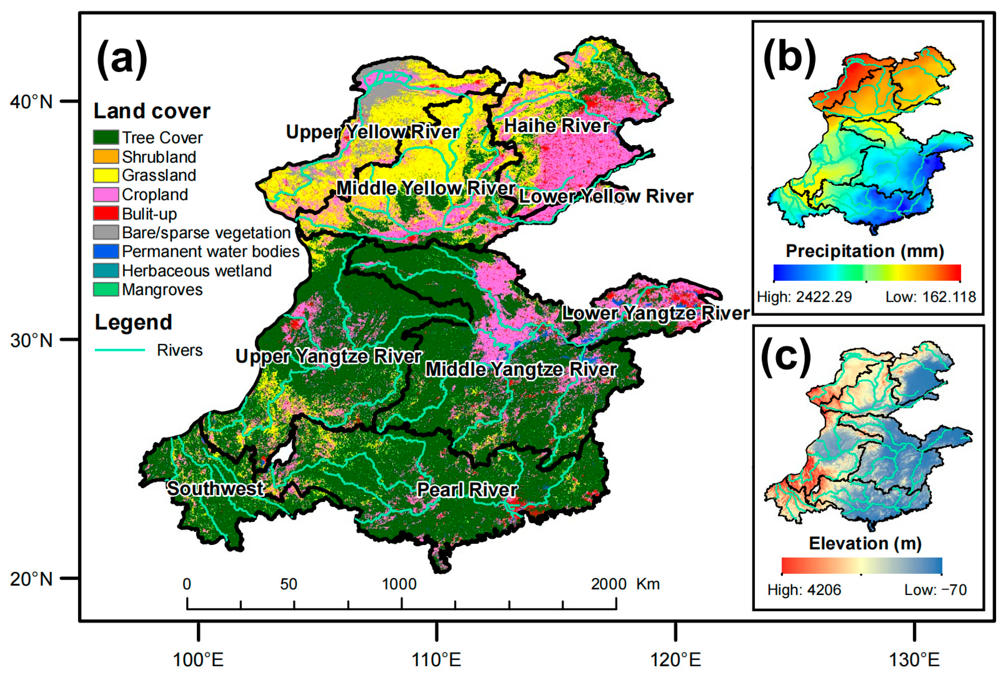
2. Study Regions and Data

This study focuses on China’s five basins, i.e., the Yangtze River Basin, the Yellow River Basin, the Pearl River Basin, the Haihe River Basin, and the Southwest River Basin, excluding the Tibetan Plateau region. These basins span across eastern, northern, southern, and southwestern China. The Yangtze River Basin supports 40% of the population and one-third of the national Gross Domestic Product [38]; the Yellow River Basin sustains 12% of the population and 15% of the irrigated agriculture area [39]; the Pearl River Basin drives economic growth and ecological protection in southern China [40]; the Haihe River Basin includes the Beijing–Tianjin–Hebei region and 10% of the national grain production [41,42]; and the Southwest River Basin is crucial for hydropower generation [43]. To account for the large size and diverse geographical and climatic conditions of the Yangtze River Basin and the Yellow River Basin, these two basins were further subdivided into the upper, the middle, and the lower reaches. Therefore, this study examines nine basins in total: the Upper Yangtze River Basin, the Middle Yangtze River Basin, the Lower Yangtze River Basin, the Upper Yellow River Basin, the Middle Yellow River Basin, the Lower Yellow River Basin, the Pearl River Basin, the Haihe River Basin, and the Southwest River Basin.

The datasets used in this study were sourced from various publicly accessible databases. A summary of these datasets is provided in

Table 1. List of data sets used in this study.

Variable	Product	Spatial Resolution	Temporal Resolution
SM	ESA CCI	0.25°	Daily
SM	ERA5-Land	0.1°	Daily
Air Temperature	ERA5-Land	0.1°	Daily
SSRD	ERA5-Land	0.1°	Daily
Runoff	ERA5-Land	0.1°	Daily
Precipitation	ERA5-Land	0.1°	Daily
ET	GLEAM	0.1°	Daily
Elevation	SRTM	90 m	/
Soil Texture	OpenLandMap	250 m	/
PDSI	TerraClimate	4 km	Monthly
Land Cover	ESA WorldCover	10 m	Annual
Precipitation	GPM	0.1°	3-hourly

.

2.1. Soil Moisture Data Set

The soil moisture dataset used in this study was obtained from the ESA CCI. Specifically, we utilized the most recent version (09.1) of the daily combined active-passive SM products, covering the period from 1980 to 2023 at a spatial resolution of 0.25°. This product integrates soil moisture retrievals from both active and passive microwave sensors, resulting in a robust and comprehensive dataset suitable for long-term analysis. To align with the temporal resolution required for our analysis, the daily SM data were aggregated into eight-day intervals by calculating the mean values for each period. This compositing scheme divided each year into 46 regular intervals, with the final interval containing 5 or 6 days depending on whether the year was a leap year.

2.2. Data Sets for SM Gap Filling

To address the gaps in the ESA CCI SM product, we incorporated four additional datasets: ERA5-Land, the Global Land Evaporation Amsterdam Model (GLEAM), the Shuttle Radar Topography Mission (SRTM) Digital Elevation Data Version 4, and the OpenLandMap Soil Texture Class (USDA System). To ensure spatial consistency as ESA CCI SM, all datasets for SM gap filling were resampled to a 0.25° resolution using bilinear interpolation for continuous variables and nearest-neighbor interpolation for categorical data.

ERA5-Land is a reanalysis dataset that integrates observational and model data to provide land surface information at a spatial resolution of approximately 0.1°. Compared to other reanalysis products, NCEP/NCAR with a spatial resolution of 2.5°, JRA-55 with 1.25°, and MERRA-2 with 0.5°, ERA5-Land provides the highest spatial resolution and uses more advanced data assimilation technology [44]. It offers a globally complete dataset spanning from 1950 to the present, making it a valuable resource for historical climate analysis [45]. For this study, we used five key variables from ERA5-Land: volumetric soil water content in the topsoil layer (0–7 cm), 2 m air temperature, surface solar radiation downwards (SSRD), runoff, and total precipitation. These variables were collected daily across the study area from 1980 to 2023 at a spatial resolution of 0.25°. To maintain temporal consistency with the SM data, the daily data were aggregated into eight-day intervals.

The GLEAM provides terrestrial evapotranspiration (ET) estimates on a daily basis from 1980 to the present by integrating satellite-based climate and environmental data [46]. Compared to other global ET products such as MOD16 and GLDAS, GLEAM demonstrates superior performance with the lowest uncertainty and higher correlation with in situ measurements, particularly showing excellent accuracy in forest and grassland land cover types [47]. We collected the daily actual ET data from the latest version of GLEAM (version 4.1a) from 1980 to 2023, at a 0.25° spatial resolution.

The SRTM Version 4 provides elevation information between 60°N and 56°S with 90 m spatial resolution, collected during an 11-day mission in February 2000, with enhanced consistency and integrity through the gap-filling processes [48]. Compared to other global elevation products such as ASTER, SRTM Version 4 demonstrates better performance in characterizing micro-topography and has a hydrologic network with higher accuracy, especially in areas with low to medium relief [49]. The OpenLandMap offers soil texture information at a fine spatial resolution of 250 m for the 0 cm depth layer, representing soil conditions up to 2018 [50]. We selected this dataset for its comprehensive global coverage and high spatial resolution. All these datasets were resampled to match the 0.25° spatial resolution for soil moisture.

2.3. Data Sets for Identifying Drought Events

The Palmer Drought Severity Index (PDSI) was collected from TerraClimate to assess drought severity. The TerraClimate dataset is a global monthly dataset that offers land surface climate and water balance variables. It combines high-resolution climate normals from the WorldClim dataset with coarser time-varying data from sources such as CRU Ts4.0 and the Japan 55-year reanalysis (JRA55) [51].

Historical drought records for the nine study basins were collected from the Chinese National Climate Center. These records include detailed information on the start and end months of each drought occurrence, providing a temporal framework for analyzing drought events across the basins.

2.4. Land Cover and Precipitation

As illustrated in Figure 1, the nine basins in the study area exhibit diverse land cover types, distinct precipitation and elevation patterns, with river networks showing water movement patterns across the basins. To analyze these spatial characteristics, we obtained land cover data from ESA’s WorldCover 2021 product, which provides global land cover maps at a high spatial resolution of 10 m [52]. The dataset includes nine distinct land cover classes: tree cover, shrubland, grassland, cropland, built-up areas, bare/sparse vegetation, permanent water bodies, herbaceous wetlands, and mangroves.

Precipitation data were sourced from the Global Precipitation Measurement (GPM) mission, which generates global precipitation estimates every three hours [53]. For this study, we calculated the annual mean precipitation across the study area at a 1 km resolution to complement the land cover analysis. Additionally, elevation data were obtained from the SRTM Version 4 at a 90 m resolution.

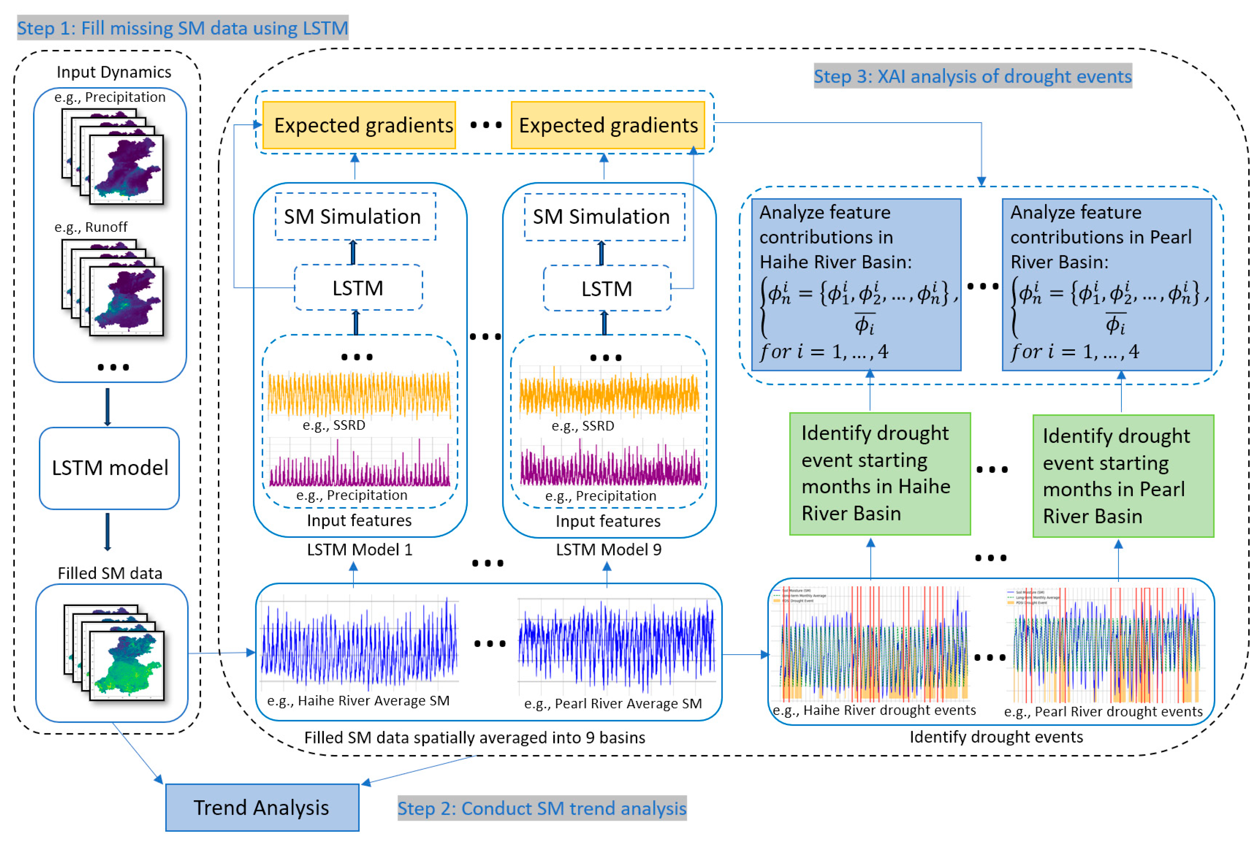
3. Materials and Methods

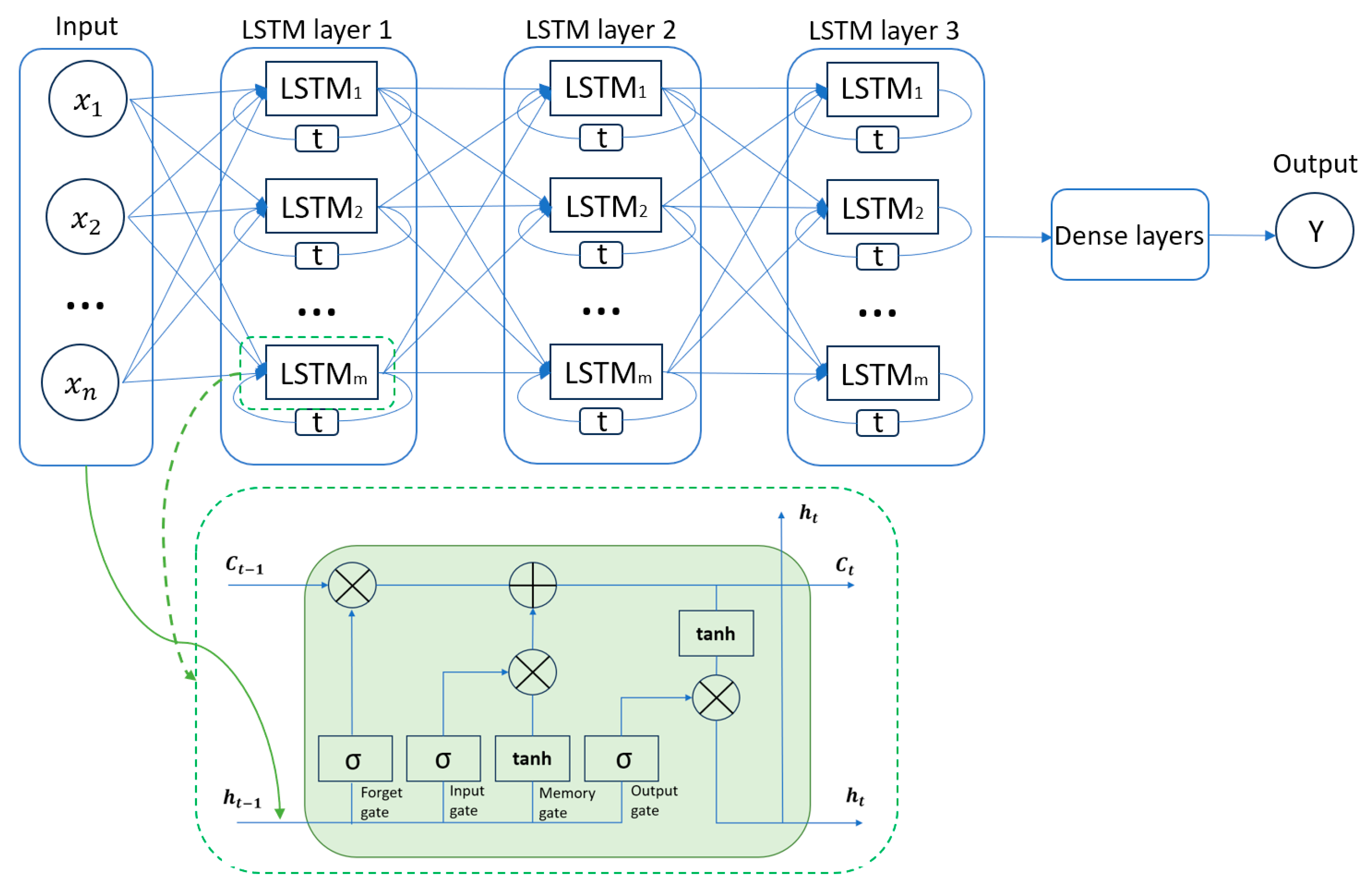
This study employed a structured approach to achieve three primary objectives, as illustrated in Figure 2. The first step involved addressing the missing values in the ESA CCI SM dataset, which was provided at eight-day intervals for the nine basins from 1981 to 2023. An LSTM model was utilized to reconstruct the missing values, leveraging its ability to capture temporal dependencies in the time series data. This step produced a continuous and reliable SM dataset, which served as the foundation for subsequent analyses. Using the reconstructed SM dataset, we conducted a 43-year trend analysis to investigate the long-term variability across the study area. This analysis identified spatial and temporal patterns in SM trends, providing insights into regional differences and enabling a deeper understanding of the mechanisms driving droughts. To assess the factors contributing to SM changes during drought events, we applied the Expected Gradient (EG) method, an explainable artificial intelligence approach. This method is grounded in SHapley Additive exPlanations (SHAP) values, allowing us to quantify the relative contributions of the key hydrometeorological variables to SM variability.

3.1. LSTM

The LSTM network is a specialized type of Recurrent Neural Network (RNN) designed to efficiently learn and model long-term dependencies in sequential data [54]. This capability makes LSTM particularly well-suited for time series applications, as it addresses the problem of vanishing gradients commonly encountered in classical RNNs [55]. The architecture of the LSTM model used in this study is depicted in Figure 3 and comprised several key components: input features, multiple LSTM layers, a fully connected (dense) layer, and a final output layer. In this framework, the input features consisted of a time series of hydrometeorological variables. These variables were fed into the stacked LSTM layers, which were designed to capture both short- and long-term dependencies within the data. The dense layer subsequently processed the extracted features from the LSTM layers to facilitate the final prediction at the output layer. This architecture ensured a robust representation of the temporal patterns in the hydrometeorological data, making it a powerful tool for time series prediction tasks.

In each LSTM layer, the model relied on the architecture of the LSTM cells to learn the input feature sequence data patterns. As shown in Figure 3, a single LSTM cell consisted of three input streams, including the previous hidden state ($h_{t-1}$), the previous cell state ($C_{t-1}$), and the current input features ($X_t$). Based on the current input and the previous hidden state, a multilayer perceptron was used to calculate four internal gates, including the forget gates ($F_t$), input gates ($I_t$), candidate cell states ($\widetilde{C_t}$), and output gates ($O_t$). These gates determined the information to be retained, updated, or discarded as the sequence progresses. The $F_t$ determined which information to discard from the cell state:

$$F_t=\sigma (W_{fx}{X}_t+W_{fh}{h}_{t-1}+b_f),$$

(1)

where $\sigma$ is the sigmoid function, $W_f$ represents the forget gate weights, and $b_f$ is the forget gate bias. The $I_t$ decided which new information would be stored in the cell state:

$$I_t=\sigma \left(W_{ix}{X}_t+W_{ih}{h}_{t-1}+b_i\right),$$

(2)

where $W_i$ represents the input gate weights and $b_i$ is the input gate bias.

The previous cell state was then updated by applying the forget gate, input gate, and the candidate cell state ($\widetilde{C_t}$) to produce a new cell state ($C_t$). The output of the cell ($O_t$) was determined by the output gate, which controls how much of the cell state is passed on to the next time step. The mathematical workflow of the LSTM can be summarized as follows [56], where $W$ denotes the weight matrices and $b$ represents the bias terms, both optimized during model training.

$$\widetilde{C_t}=\tanh \left(W_{\tilde{c}x}{X}_t+W_{\tilde{c}h}{h}_{t-1}+b_{\tilde{c}}\right),$$

(3)

$$O_t=\sigma \left(W_{Ox}{X}_t+W_{Oh}{h}_{t-1}+b_O\right),$$

(4)

$$C_t=F_t\times C_{t-1}+I_t\times \widetilde{C_t},$$

(5)

$$h_t=O_t\times \tan h\left(C_t\right),$$

(6)

$$y=W_d{h}_T,$$

(7)

The hyperparameters for the LSTM models in this study were determined through empirical testing based on model performance and convergence behavior. To fill the gaps in the ESA CCI SM data, we developed an LSTM model with an architecture consisting of three LSTM layers, each with 256 hidden cells, followed by a dense layer for output. A dropout rate of 0.3 was applied between the LSTM layers to prevent overfitting. The input feature data consisted of eight variables over the study area including temperature, SSRD, precipitation, ET, runoff, volumetric soil water content in the topsoil layer, elevation, and soil-texture class. The temporal resolution was eight days from 1980 to 2023, so the time series consisted of 2024 values. The spatial resolution was 0.25°, so the grid shape of the study area (containing nine basins) was 90 × 97. Therefore, the input layer received features with a shape of 90 × 97 × 8, where each feature provided a sequence of 46 time steps. Considering the lagged influence of environmental variables on SM, the prediction of the i-th SM value required a sequence of auxiliary data from time step i-46 to i-1 (approximately one year). This explains why the gap-filling process started from 1981, as predictions for early 1981 required the auxiliary data sequence from 1980.

The input data were randomly divided into 8:1:1 for training, validation, and test purposes. The LSTM model captured the temporal dependence of the entire sequence and effectively learned how these variables interact with each other over time to predict the SM. The model was trained using the Adam optimizer and the model parameters were iteratively updated using the training samples. The initial learning rate was 0.001, the batch size was 64, and the maximum number of training sessions was 100. To prevent overfitting, the dropout was used between the LSTM layers and training was stopped early if the validation loss did not improve within four epochs to ensure that the model did not overfit the training data.

After filling in the data gaps, we used the supplemental SM data to develop LSTM models to simulate SM in each of the nine basins individually, focusing only on hydrometeorological variables including precipitation, temperature, SSRD, and ET. These variables were derived from the same data resources used for the SM gap-filling process. In the task of constructing SM simulation models, we averaged all pixels within each basin to represent the overall basin conditions, rather than maintaining the original spatial resolution. This spatial averaging approach allowed us to focus on the overall hydrometeorological conditions in each basin. SM data were also reprocessed to be consistent with the spatial and temporal resolution of the hydrometeorological variables, ensuring consistency of the dataset used for interpretable deep learning models.

For each simulation, the input data were shaped as 2024 × 4 where 70% of the input data were used for training purposes and the remaining data were used for testing purposes. Subsequently, this 70% was further divided into training and validation sets with a ratio of 7-to-3. Unlike the gap-filling model which had a larger dataset allowing for an 8:1:1 split ratio, the SM simulations for each basin used a smaller dataset. Thus, these models required larger proportions for validation and testing to ensure robust model evaluation and to prevent overfitting. The LSTM models for each basin consisted of three LSTM layers with 256 hidden cells each, followed by a dense layer for outputting the SM predictions. The model was compiled using the Adam optimizer with a learning rate of 0.0001. Due to the small dataset, a batch size of four was chosen and the model was trained for a maximum of 200 epochs. Dropout was applied to prevent overfitting and early stopping was used with a patience of 30 epochs. Model checkpoints were also applied to preserve the best performing models during training.

We used several common statistical metrics: R-squared (R²), Nash–Sutcliffe efficiency (NSE), mean absolute error (MAE), and root mean square error (RMSE) to evaluate the performance of the LSTM models. The application of each metric depended on the tasks of the models.

3.2. The Interpretable Method for the Deep Learning Model

The EG method is a gradient-based XAI technique that quantifies the contribution of each input feature by leveraging the model’s gradients [57]. It extends the Integrated Gradients method by averaging the model’s output gradients over multiple baseline inputs, thereby providing more robust and reliable explanations for feature importance. EG is a feature attribution method that satisfies key interpretability axioms for neural networks, including completeness and implementation invariance [58]. This makes it suitable for explaining complex differentiable models regardless of their specific architecture. EG calculates the effect of each feature on the model’s predictions by evaluating how the predictions change as the input transitions from a baseline value to the actual value. By averaging these gradients over different baseline inputs, the method accounts for variations in feature interactions and ensures more comprehensive attribution of feature importance [58]. When integrated with an LSTM network, EG quantifies how each input feature contributes to the prediction over the entire time series. Thus, important features in SM dynamics over time can be explained and can provide an important basis for understanding the mechanisms of drought development.

In this study, input feature data were selected from the six months preceding the onset of drought events to account for the delayed effects of hydrometeorological conditions on soil moisture. Four primary input features were used: precipitation, temperature, SSRD, and ET. To evaluate the contributions of these features to the LSTM model’s SM predictions during drought events, SHAP values were computed using the EG method. The function can be summarized as [29]:

$${\varphi }_{{EG}_i}\left(x\right)={\mathbb{E}}_{x^{\prime }~D,\alpha ~U\left(\mathrm{0,1}\right)}[(x_i-x_i^{\prime })·{\displaystyle \frac{\partial f(x^{\prime }+\alpha (x-x^{\prime }\left)\right)}{\partial x_i}}].$$

(8)

where ${\varphi }_{{EG}_i}\left(x\right)$ represents the SHAP value for feature $i$, calculated using EG as a given input $x$. The term $x_i^{\prime }$ is the baseline value for feature $i$, drawn from a distribution $D$, and ${\displaystyle \frac{\partial f}{\partial x_i}}$ is the gradient of the model’s output with respect to feature $i$. The interpolation parameter $\alpha$ controls the weighting of the baseline and the input, and the expectation $\mathbb{E}$ is taken over multiple baseline samples to ensure robust attribution.

To investigate the causes of drought events, we utilized the EG method to interpret the SM model simulated by the LSTM network. The model was developed using input features observed up to six months prior to the onset of each drought event. This six-month lead time was selected based on previous studies highlighting the delayed effects of hydrometeorological conditions on SM dynamics [59]. By examining the EG results, we assessed the significance and variability of four input features during the months leading up to drought onset.

3.3. Trend Analysis

We calculated soil moisture trends across the nine basins from 1981 to 2023. Initially, we applied Seasonal and Trend decomposition using Loess (STL) to the SM time series data. STL effectively separated the data into three components: long-term trends, seasonal patterns, and irregular variations. This decomposition enabled us to focus on the underlying trends in SM by filtering out periodic seasonal influences and residual noise, ensuring a clear view of long-term changes. After isolating the trend components, we quantified the rate of change in SM over time using Theil–Sen regression. This nonparametric method estimates the median slope of the trend, offering resilience against outliers that can skew results in ordinary least squares regression. Theil–Sen regression provided a decadal rate of SM change, offering insights into basin-wide and grid-level trends over the 43-year analysis period. To evaluate the statistical significance of the identified trends, we employed the Mann–Kendall (MK) test. The MK test is a widely used nonparametric method for detecting monotonic trends in time series data, requiring no assumption about the data’s underlying distribution [60]. By applying this test, we obtained p-values for each trend estimate, setting a significance threshold of p < 0.05. Trends meeting this criterion were deemed statistically significant and included in our final analysis, while non-significant trends were excluded.

3.4. Identification of Droughts

To identify the drought events in the nine basins from 1981, we utilized the monthly SM data from the gap-filled ESA CCI SM dataset, averaged across each basin. Our identification methodology drew on previously validated methods for identifying drought events based on hydrological deficits. And, we further incorporated historical drought records to validate the identified drought events, ensuring the reliability of our drought detection. In the GRACE-based hydrological drought characterization study [61], the water storage deficit approach established that drought events could be effectively characterized through continuous storage deficits and their duration. This concept was further validated in a study of drought monitoring [62], where drought identification was applied to the Yangtze River Basin through integrating multiple drought indicators. The study successfully identified extreme drought periods using the combined criteria of PDSI values below −2 and soil moisture deficits exceeding 20% of the climatology, both persisting for six consecutive months.

Based on previously established frameworks, we constructed our drought identification method by integrating SM variations and PDSI criteria. The ESA CCI SM dataset provided SM values ranging from 0–1 m³m⁻³, representing the ratio of water volume to soil volume. Under this standardization, even small variations in SM values could be significant for drought detection. Therefore, we defined drought events as periods when at least two consecutive monthly SM values were more than 5% below the 43-year monthly average for the respective basin. In conjunction with the criteria of SM variations, we also required the PDSI value to be below −2 for the same two consecutive months to indicate moderate to severe drought conditions [63], ensuring both the SM deficit and meteorological drought conditions were met simultaneously.

To further enhance the reliability of our drought identification, we compared our results with historical drought records from the Chinese National Climate Center and the China Hydrological Yearbook published annually by the Ministry of Water Resources of China [64]. From our identified drought events, we selected those that overlapped with the severe drought events documented in these historical records, ensuring that our analyses were accurate, valid, and focused on the most severe drought periods.

To evaluate the robustness of our drought identification method, we conducted sensitivity analysis on the key threshold parameters. Results showed that adjusting the SM deficit threshold (±1%), consecutive months threshold (±1 month), as well as the PDSI threshold (±0.5), had a minimal impact on drought detection, with over 90% of drought events consistently identified across the different parameter combinations. This demonstrates the stability of our drought identification approach despite threshold variations.

4. Results

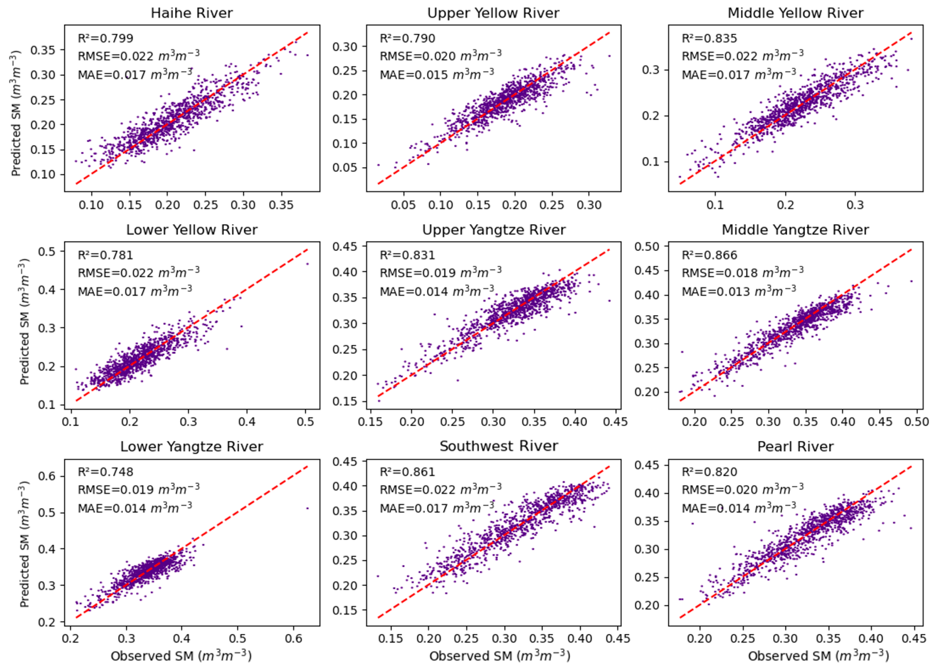
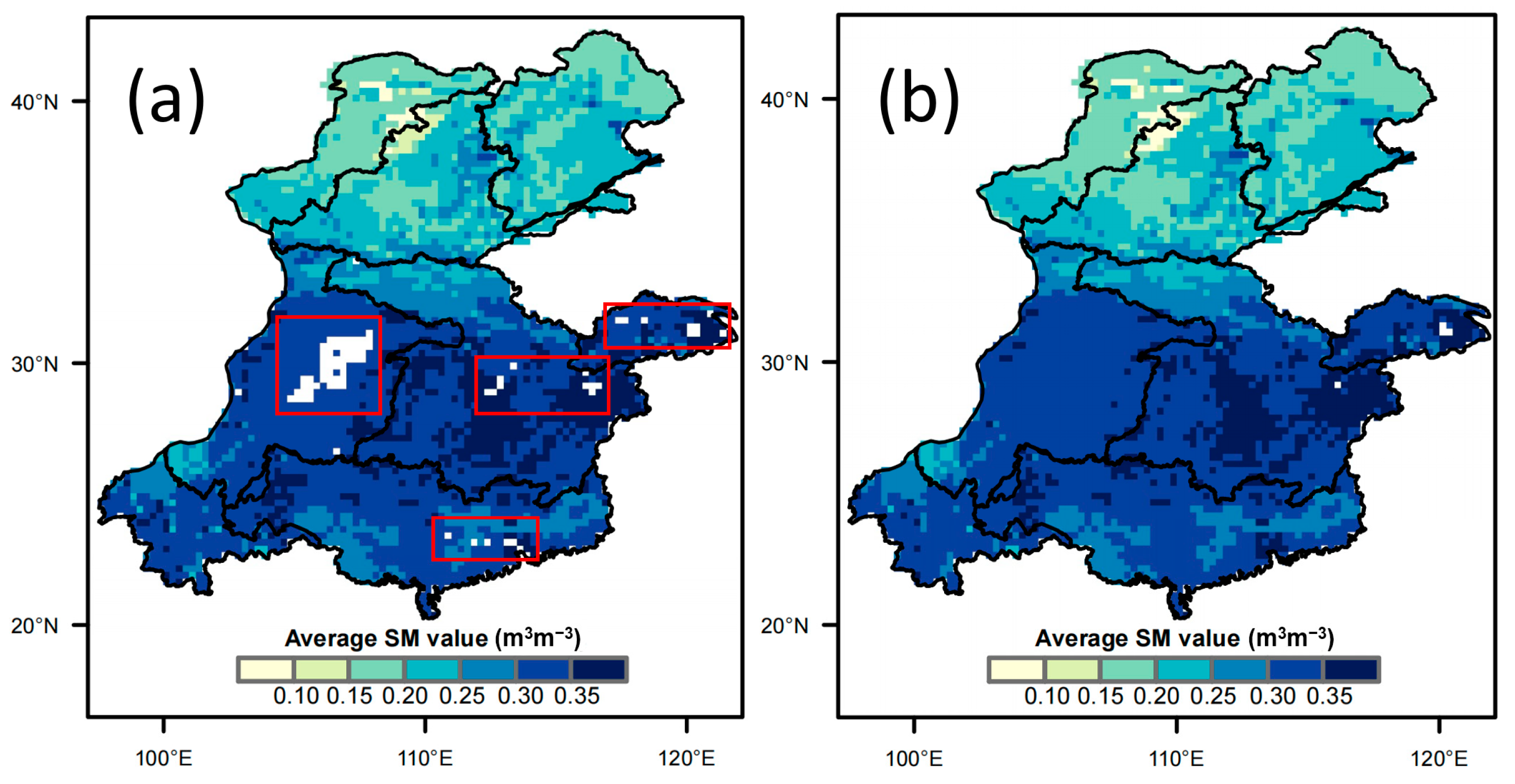
4.1. LSTM-Based ESA CCI SM Data Gap Filling

The LSTM model successfully addressed gaps in the ESA CCI SM dataset, achieving high accuracy in reconstructing the SM values. The model achieved an R² of 0.928, with a RMSE and a MAE of 0.02 and 0.015 m³m⁻³, respectively. To evaluate the model consistency across basins, 1000 random samples from each basin’s test dataset were analyzed. Figure 4 illustrates the model performance in each basin. The highest R² was observed in the Middle Yangtze River Basin (R² = 0.866), while the Pearl River Basin showed a median R² of 0.820. The lowest R² was in the Lower Yangtze River Basin (R² = 0.748). Despite these regional variations, the model demonstrated robust performance across all basins, maintaining low RMSE and MAE values.

The spatial distribution of the SM data before and after gap filling was also assessed. Figure 5a shows the temporal average (1981–2023) of the original SM data distribution, where certain basins, notably the Yangtze River Basin, exhibited significant data gaps, as highlighted by the outlined areas in red with missing grid points. After gap filling, as shown in Figure 5b, most gaps were resolved, significantly improving data coverage. This enhancement ensured comprehensive spatial representation, reducing uncertainties in subsequent analyses.

Figure 6a depicts the availability of the original SM data at each grid point across the time series, with an initial overall availability of 76.89%, indicating approximately one-quarter of the data was missing. Following gap filling, Figure 6b demonstrates a marked improvement, with the overall availability rising to 99.31%. This substantial increase provided a more complete dataset for time series analysis. Figure 6c highlights the temporal evolution of data availability over the study period. Before 2007, data gaps were more severe, likely due to limitations in remote sensing technology and sensor coverage. Seasonal variations in data gaps were also evident, potentially caused by weather conditions affecting satellite observations, such as cloud cover or snow [16]. After the gap-filling process, data availability improved consistently across all years and seasons, resulting in a high-quality dataset suitable for detailed analysis.

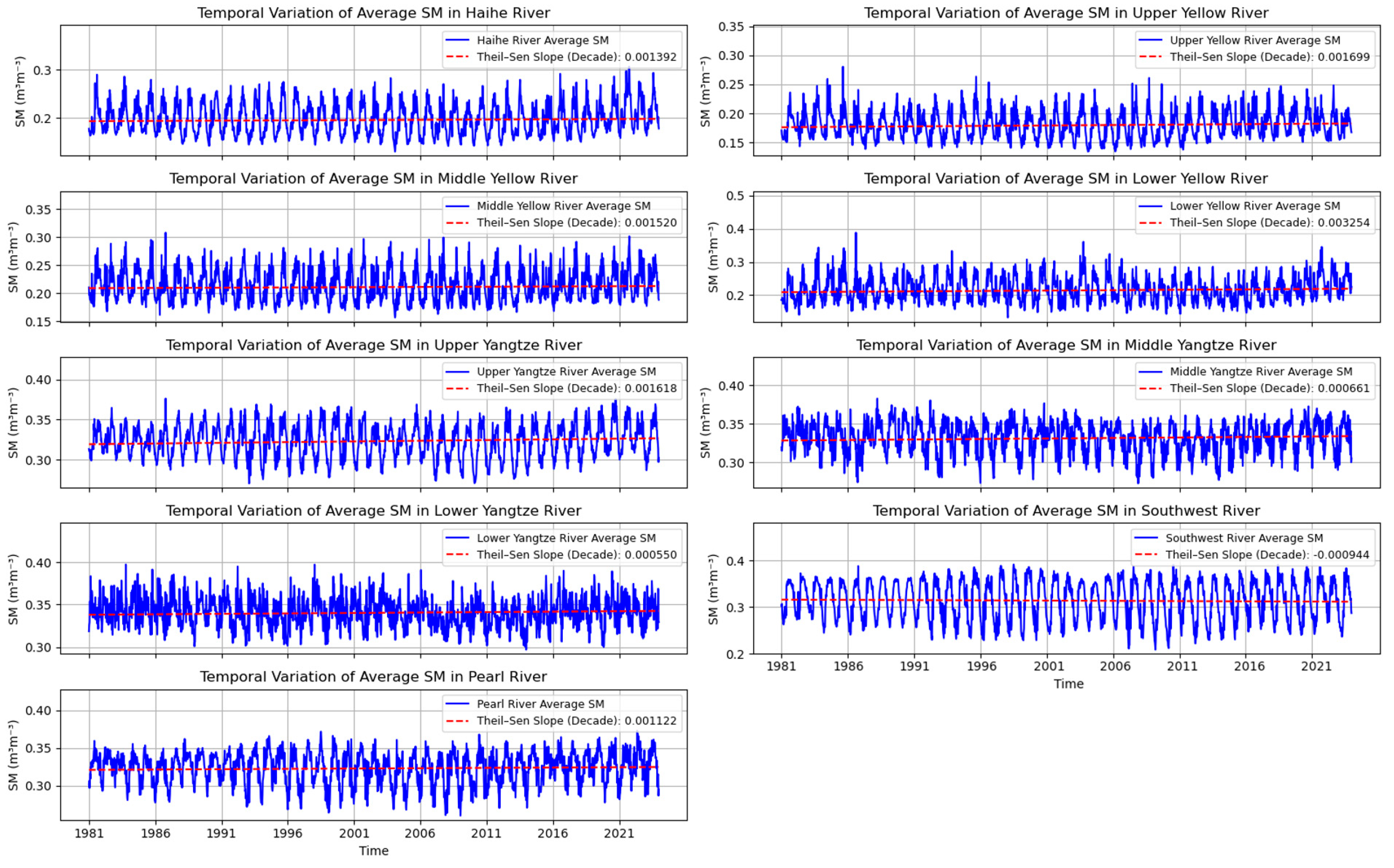
4.2. The Long-Term SM Trend

The analysis of soil moisture values from 1981 to 2023 revealed distinct variations among the basins and temporal variations across the nine major basins in China, as illustrated in Figure 7. The Yangtze River Basin, Southwest River Basin, and Pearl River Basin demonstrated notably higher SM values, whereas the Haihe River Basin and Yellow River Basin showed relatively lower values. This spatial pattern coincided with precipitation distributions depicted in Figure 1, where greater precipitation occurred in the southern regions. The temporal variations showed pronounced seasonal fluctuations in all basins. The long-term changes remained modest, as evidenced by the small magnitude of Theil–Sen slope values.

The Theil–Sen slope estimates indicated varied trends in SM changes across basins over the 43-year period. Most basins exhibited a positive trend, with the northern regions experiencing more pronounced increases. The Lower Yellow River Basin showed the most substantial increase, with a slope of 3.06 × 10⁻³ m³m⁻³/decade, followed by moderate upward trends in the Upper and Middle Yellow River Basins, the Haihe River Basin, the Upper Yangtze River Basin, and the Pearl River Bain (slopes between 1.12 × 10⁻³ and 1.70 × 10⁻³ m³m⁻³/decade). The Middle and Lower Yangtze River Basin showed minimal increases (6.61 × 10⁻⁴ and 5.50 × 10⁻⁴ m³m⁻³/decade, respectively). The Southwest River Basin was unique in showing a slight decline in SM levels, with a slope of −9.44 × 10⁻⁴ m³m⁻³/decade. The northern basins showed more substantial increases with an average slope of 1.97 × 10⁻³ m³m⁻³/decade, while the southern basins exhibited smaller changes with an average slope of 6.01 × 10⁻⁴ m³m⁻³/decade. This pattern suggests that regions with abundant precipitation, such as the south, tend to maintain stable SM conditions, while the drier northern regions show a greater potential for SM variability.

Further analysis was conducted to better understand the basin-scale drought evolution by examining SM trends across different land cover types, as land cover characteristics provide insights into the spatial features of basins that complemented our temporal analysis. The analysis (Figure 8) revealed distinct SM trends linked to specific land cover categories. The southern basins, such as the Yangtze River Basin, Southwest River Basin, and Pearl River Basin, which have higher SM values and smaller variations in trends, were predominantly characterized by forests with a high proportion of tree cover. In contrast, the northern basins, with lower SM values and greater trend variations, were dominated by grasslands and croplands with less tree cover. The land cover-specific analysis highlighted that grasslands and shrublands exhibit the most positive SM trends, whereas croplands display the most negative trends. Tree cover and bare or built-up areas showed slight negative trends, but these declines were not substantial. This indicated a strong correlation between SM trends and land cover types within each basin. On the other hand, SM trends were more spatially concentrated in the northern regions, with negative trends primarily observed in cropland areas. Conversely, the southern basins displayed a more dispersed spatial pattern of SM declines. Interestingly, while the Southwest and Pearl River Basins had similar land cover profiles, the Southwest River Basin showed a large-scale negative SM trend despite its lower proportion of farmland. This discrepancy suggests that land cover alone cannot fully explain SM trends, highlighting the complex interactions between multiple factors influencing SM dynamics.

4.3. Attribution of Drought Events

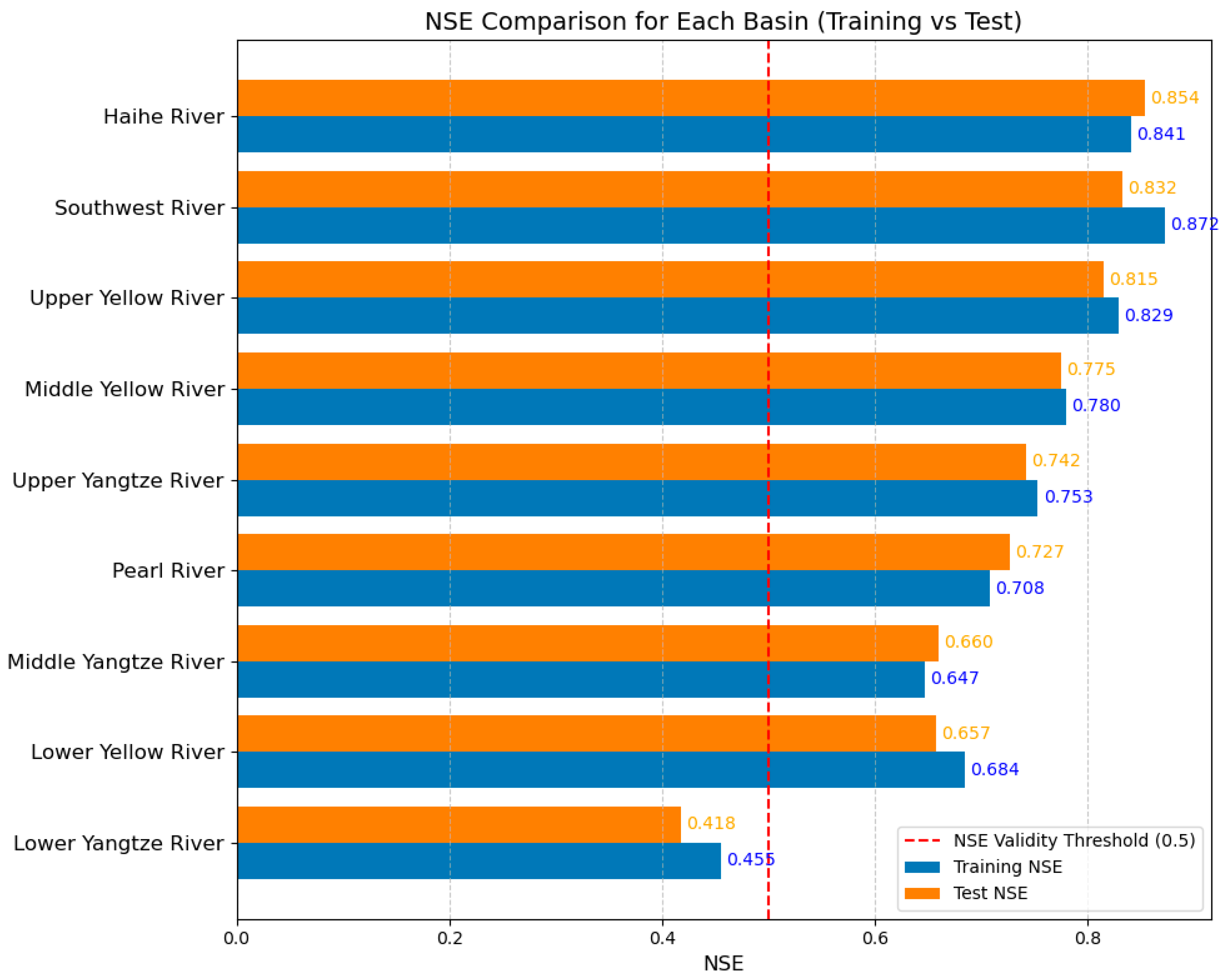
4.3.1. LSTM Model Performance

From 1981 to 2023, a total of 26 drought events were identified across the nine basins in the study area. These events were distributed as follows: four in the Haihe River Basin, three in the Upper Yellow River Basin, five in the Middle Yellow River Basin, three in the Lower Yellow River Basin, one in the Upper Yangtze River Basin, three in the Middle Yangtze River Basin, three in the Lower Yangtze River Basin, three in the Southwest River Basin, and one in the Pearl River Basin. These drought events were analyzed using the LSTM model in combination with the EG method.

To assess the performance of the LSTM model in delineating SM dynamics, separate models were trained and tested for each of the nine basins. As shown in Figure 9, the average NSE values for most basins exceeded this threshold, except for the Lower Yangtze River Basin, where the NSE value was slightly below 0.5. This result suggested that the SM dynamics in the Lower Yangtze River Basin are less influenced by the selected hydrometeorological variables. Nonetheless, the relatively low MAE and RMSE values, combined with a test dataset NSE of 0.455, demonstrated that the model was still able to reasonably capture the effects of hydrometeorological factors on SM in this basin. For the other basins, the model exhibited strong performance, with MAE and RMSE values consistently lower, and NSE values ranging from 0.647 to 0.872 during the training phase and from 0.657 to 0.854 during the testing phase. These results confirmed the robustness of the LSTM model in simulating SM dynamics across diverse regions, capturing the complex interactions between hydrometeorological factors and SM variations effectively.

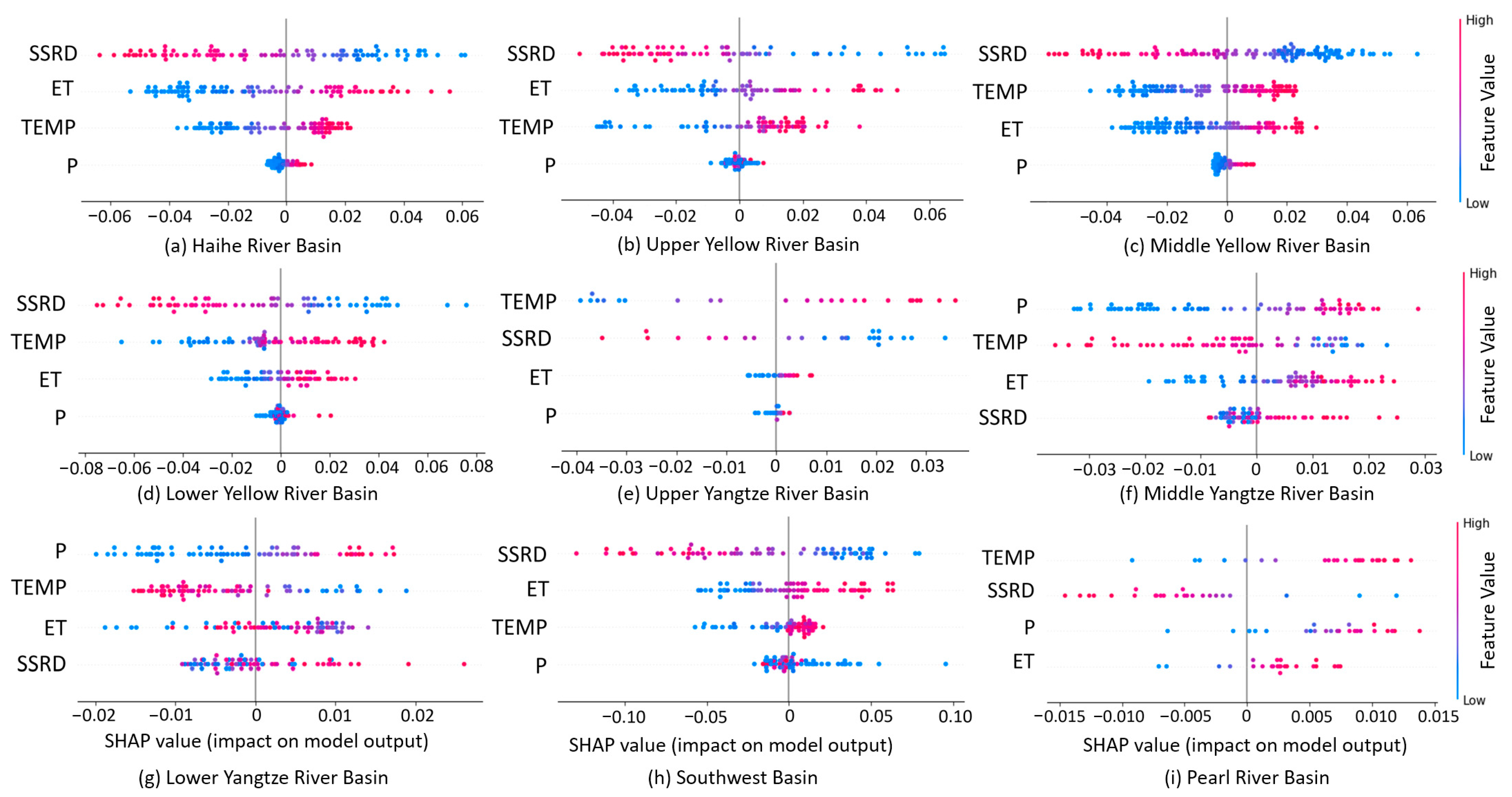
4.3.2. The Attribution of Hydrometeorological Drivers in Drought Events

We employed SHAP values, derived from the EG method, to interpret the contribution of key features (i.e., precipitation, temperature, SSRD, and ET) to SM dynamics during defined drought events. The analysis modeled SM dynamics for six months preceding the onset of each drought event. Figure 10 presents the SHAP-based interpretability analysis for all identified drought events across the nine basins. Notably, the mean SHAP values were higher in the northern basins compared to the southern basins, indicating a stronger influence of meteorological drivers on droughts in the northern regions. In basins such as the Haihe, Upper Yellow River, Middle Yellow River, Lower Yellow River, Southwest, and Pearl River, high SSRD emerged as the dominant factor driving droughts. Additional factors, including low ET, temperature, and precipitation, also contributed to reduced SM levels, though precipitation had a minimal effect in these basins. In contrast, in the Upper Yangtze River Basin, droughts were primarily driven by low temperatures and high SSRD. The dominance of SSRD in semi-humid and semi-arid regions, (e.g., Haihe and Yellow River Basins) aligns with the limited precipitation and increased susceptibility to radiation-driven soil drying. Interestingly, the Pearl River Basin, despite its high precipitation and dense tree cover, also experiences droughts predominantly driven by SSRD. Conversely, in the Middle and Lower Yangtze River Basins, droughts were primarily attributed to low precipitation and high temperatures, with SSRD exerting minimal influence.

Overall, high SSRD and low precipitation were identified as the principal precursors to SM decline anomalies, as predicted by the LSTM model. This underscores the strong interaction between these features in driving drought events. These findings are consistent with previous studies, which have shown that droughts are often triggered by reduced precipitation and exacerbated by extreme climatic conditions [65,66]. Moreover, extreme events intensify the drying process, highlighting the critical role of elevated SSRD in accelerating SM depletion [67].

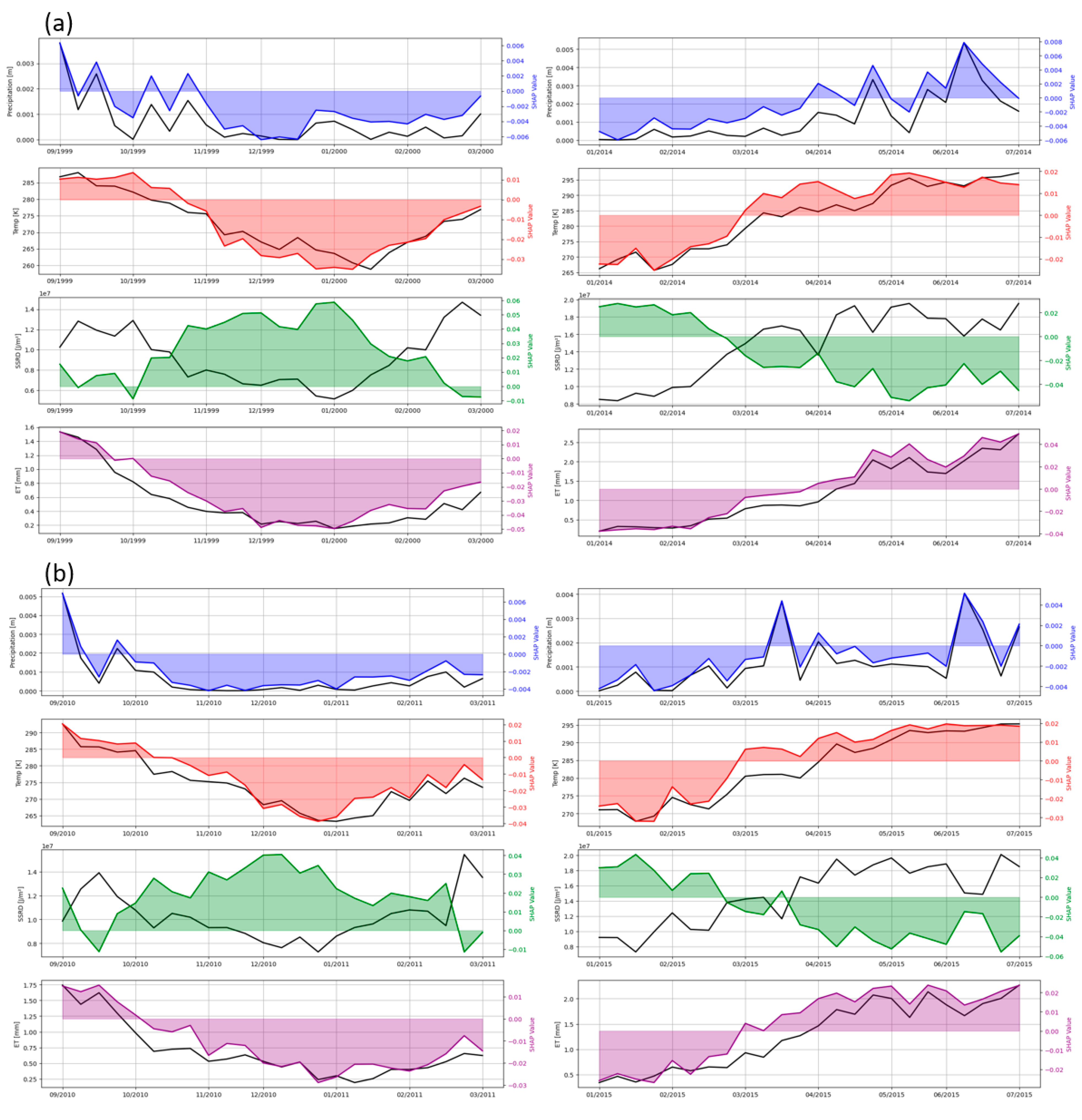
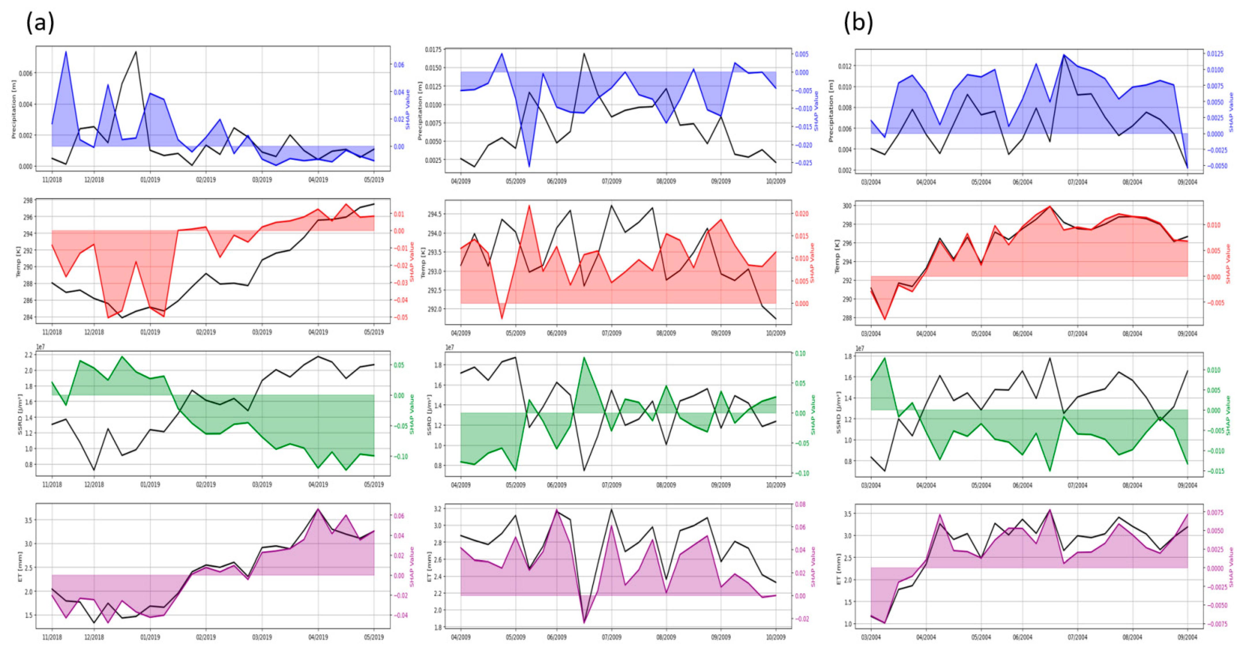
4.3.3. Attribution Analysis over a Time Scale

We conducted a detailed analysis of each drought event by examining the feature change curves and corresponding EG results for the six months preceding each drought. Representative cases are illustrated in Figure 11. In the Haihe River Basin, two drought events, one in March 2000 and another in July 2014, were analyzed. Figure 11a shows the temporal variation of the four input features (precipitation, temperature, ET, and SSRD) and their corresponding SHAP values before the droughts. Negative SHAP values indicate that the feature reduced SM, while positive values indicate an increase. For the March 2000 drought, ET exhibited the highest average SHAP value, indicating it was the dominant driver of the SM decrease, while precipitation had minimal impact. ET and temperature primarily contributed to the SM reduction during this event. Conversely, the July 2014 drought was mainly driven by high SSRD, which caused a significant decline in SM. Similar patterns were observed in the Yellow River Basin for the droughts in March 2011 and July 2015 (Figure 11b). The March 2011 drought was attributed to ET and temperature, while the July 2015 drought was driven by high SSRD.

Drought drivers varied significantly by season in the Haihe and Yellow River Basins. Spring droughts (e.g., March events) were mainly influenced by reduced ET and temperatures. During spring, temperatures and solar radiation limit ET, making it the primary driver of SM declines [68]. In contrast, summer and autumn droughts (e.g., events between June and September) were predominantly driven by high SSRD, which exacerbates ET and increases SM susceptibility to radiation-induced drying [69]. This seasonal contrast highlights the distinct hydrometeorological dynamics: spring droughts are primarily ET-driven, while summer and autumn droughts are predominantly SSRD-driven.

In the Middle and Lower Yangtze River Basins, the seasonal patterns of drought drivers were also evident (Figure 12). In the Middle Yangtze River Basin, two drought events (April 2011 and October 2013) were analyzed. The April 2011 drought was primarily caused by low precipitation, whereas the October 2013 drought resulted from the combined effects of low precipitation and high temperatures. Similarly, in the Lower Yangtze River Basin, the March 2011 drought was largely driven by low precipitation, while the October 2013 drought was influenced by both high temperatures and low precipitation. Unlike other basins, SM decreases in the Yangtze River region were particularly sensitive to precipitation deficits. In spring, precipitation alone was the primary driver of SM decline, while autumn droughts were influenced by a combination of precipitation and temperature. This underscores the unique climatic dynamics of the Yangtze River region, where drought drivers transition from precipitation dominance in spring to multifactor influences in autumn.

The Southwest and Pearl River Basins exhibited different patterns compared to the Haihe and Yellow River Basins. Unlike the strong seasonality observed elsewhere, drought drivers in these basins were relatively consistent across seasons. Figure 13 shows that high SSRD was the primary factor driving SM declines in both basins, irrespective of the season. Other factors, such as ET, temperature, and precipitation, had a limited influence. A key characteristic of the Southwest and Pearl River Basins is their subtropical climate, marked by warm temperatures and high solar radiation throughout the year [70,71]. In the Southwest River Basin, temperature fluctuations were minimal, and consistently high SSRD levels were observed before spring droughts. This stability, coupled with strong solar radiation, makes SM in these basins more susceptible to radiation-driven drying and less responsive to seasonal variations [72]. Consequently, these basins lacked the pronounced seasonality in drought drivers observed in other regions.

5. Discussion

Our study presents a robust deep learning-based framework for filling gaps in long-term SM datasets and analyzing the drivers of droughts. We combined advanced deep learning techniques with interpretable analysis to resolve the causes of SM-related droughts, demonstrating the reliability and practical value of this framework for understanding and managing drought dynamics. By utilizing an LSTM model, we addressed missing data in ESA CCI SM records and performed a detailed examination of drought mechanisms using an interpretable machine learning approach. The EG method enhanced the transparency of the LSTM network, enabling systematic analysis of the interplay between hydrometeorological factors and droughts.

5.1. Gap-Filling Performance

Our gap-filling approach significantly advances beyond traditional interpolation and ML techniques, which often rely on assumptions of temporal or spatial homogeneity. Traditional methods like ordinary kriging, which depend solely on spatial distance relationships, lack the ability to integrate environmental variables, limiting their predictive accuracy [73]. While ML techniques such as random forest improve predictions by incorporating multi-source features, they exhibit systematic biases, underestimating SM in humid regions and overestimating it in arid areas [74]. The previous research evaluating gap-filling methods for ESA CCI SM data in China from 1982 to 2018 demonstrated that traditional ML methods showed varying performance levels. Their results showed that random forest achieved R values of 0.773, while the feedforward neural network and generalized linear model performed significantly worse [19]. To directly evaluate these methods, we conducted a comparison using our specific dataset and preprocessing methods with three widely used machine learning models: random forest (RF), gradient boosting machine (GBM), and support vector machine (SVM). As shown in Figure 14, our analysis showed that ensemble learning methods (RF and GBM) performed relatively well (R² of 0.829 and 0.819, respectively), while SVM showed notably lower accuracy (R² of 0.705). Although these results are reasonable, these methods are fundamentally limited in their inability to capture the lagged effects of environmental variables on SM dynamics. For example, the response of SM to precipitation involves temporal delays due to complex hydrometeorological processes [75].

To address this, we developed an LSTM model capable of processing time series data while integrating multi-dimensional inputs, including meteorological elements, terrain features, and the soil’s physical properties. Our model achieved superior performance, with an R² of 0.928 and RMSE of 0.020 m³m⁻³ on the test set. This represented a significant improvement in accuracy compared to both traditional interpolation methods and conventional ML techniques. Notably, it demonstrated strong generalization across diverse land cover types and climatic regions, effectively capturing the complex evolution of SM. This highlights the robustness of our approach in overcoming the limitations of traditional methods, offering a reliable solution for analyzing SM dynamics under varying environmental conditions.

5.2. Interpretability Analysis

The hydrometeorological conditions prior to drought show complex interactions. Traditional methods often rely on inductive reasoning, using predefined thresholds or general knowledge to identify drought triggers, limiting their ability to capture nonlinear interactions. Our study adopted a data-driven approach, leveraging an LSTM model to uncover the intricate relationships between hydrometeorological factors and SM dynamics. While deep learning models lack direct interpretability, explainable artificial intelligence techniques provide valuable insights into these complex relationships. By integrating XAI with LSTM outputs, we identified distinct SM drought mechanisms across the northern and southern basins, validated through basin-specific environmental conditions and prior drought knowledge. In the northern semi-arid basins, such as the Haihe and Yellow River basins, SM droughts were predominantly driven by high SSRD with seasonal characteristics. Low ET in spring drove drought conditions, while high SSRD dominated in summer and autumn, reflecting the climatic patterns of semi-arid regions. The low temperatures and reduced SSRD in spring limited ET, whereas summer and autumn were characterized by intensified SM loss due to high SSRD. The southern basins exhibited more complex drought mechanisms. In the middle and lower Yangtze River region, low precipitation drove spring SM droughts, while a combination of low precipitation and high temperatures intensified summer and autumn droughts [69,70]. In contrast, the Southwest River and the Pearl River Basins were primarily influenced by high SSRD, with no significant seasonal patterns, consistent with their subtropical climate marked by year-round warm temperatures and an elevated SSRD [76]. Our findings demonstrate that explainable DL methods effectively characterize SM drought mechanisms, highlighting regional and seasonal variability in hydrometeorological drivers.

5.3. Framework Limitations

Despite the advancements achieved in this study, several limitations should be acknowledged. Firstly, the satellite-derived datasets used, such as ESA CCI SM, GLEAM and ERA5-LAND, carry inherent uncertainties. While ESA CCI SM products offer long-term coverage and generally align with land surface models and in situ observations, they exhibit significant inaccuracies under conditions like dense vegetation and organic soils. Similarly, the GLEAM dataset shows substantial uncertainties in regions with dense vegetation, as validated against in situ measurements [77]. Additionally, while ERA5-Land provides comprehensive coverage, its accuracy is limited by systematic precipitation biases, particularly in tropical regions [78].

Since our gap-filling method relied on these satellite-derived datasets, their inherent uncertainties may have affected the performance of the model as well as the quality of the gap-filled data. The availability of auxiliary datasets also poses challenges for our gap-filling method. Particularly in the Lower Yangtze River Basin, missing data in the auxiliary datasets results in remaining gaps in our gap-filled SM data. Although these uncertainties can be assessed through in situ measurements, the limited spatial coverage and scalability of in situ observations are insufficient for validating data with large spatial and temporal coverage. Future studies could integrate multi-source in situ measurement networks and utilize bias correction methods for satellite-derived products to improve data quality.

Secondly, our deep learning framework also demonstrated varying performance across regions. For example, the lower accuracy in the Lower Yangtze River Basin suggests weaker correlations between SM and the selected hydrometeorological variables. This could reflect the influence of additional, unmodeled factors such as human activities, land use changes, and specific soil properties. The limited set of hydrometeorological variables considered in this study may not fully capture all the drivers of SM variability, reducing the model’s representational capacity in complex environments. Finally, while XAI methods provide valuable insights into the relative importance of different factors, their ability to offer detailed physical interpretations of nonlinear relationships remains limited. The EG approach effectively quantified variable importance but it may not have fully elucidated the complex interactions shaping SM dynamics.

6. Conclusions

Understanding the factors driving soil moisture dynamics during drought events is essential for unraveling the mechanisms behind cascading droughts and evaluating their impacts on agriculture, water resources, and ecosystems. This study employed deep learning models to address gaps in long-term SM datasets, enhancing the interpretability of drought drivers across major human-impacted basins in China over the past four decades.

The deep learning model demonstrated strong performance, achieving an R² of 0.928 on the test set, with low error metrics, including an RMSE of 0.020 m³m⁻³ and an MAE of 0.015 m³m⁻³. These metrics validated the model’s accuracy and reliability in reconstructing SM, substantially improving the continuity and integrity of the SM datasets required for drought analyses. Leveraging the reconstructed continuous temporal and spatial SM datasets, we examined long-term SM variations and trends across China’s major basins over the past four decades. The results revealed a slight overall increase in SM across most basins, except for the Southwest River Basin, which exhibited a marginal decline. Notably, cropland areas showed a more pronounced decline in SM compared to other land cover types, highlighting critical implications for agricultural water management.

The integration of interpretable deep learning models, particularly the EG approach, provided insights into the role of hydrometeorological variables in SM dynamics during drought events and improved the understanding of drought mechanisms. Our findings highlighted regional differences in the drivers of SM during droughts. In the northern dryland basins, drought drivers showed strong seasonal patterns, with low ET dominating spring droughts and high SSRD driving drought conditions during summer and autumn. In contrast, the southern humid basins displayed less pronounced seasonal variability. Precipitation was the primary driver in the Middle and Lower Yangtze River Basins, whereas a high SSRD emerged as the dominant factor in the Southwest and Pearl River Basins, irrespective of seasonal variation. The present findings advance the understanding of cascading drought formation across diverse climatic regions in China. Collectively, our framework provides valuable insights for improving drought mitigation strategies, sustainable water resource management, and land-use planning.

References

1. Seneviratne, S.I.; Corti, T.; Davin, E.L.; Hirschi, M.; Jaeger, E.B.; Lehner, I.; Orlowsky, B.; Teuling, A.J. Investigating soil moisture–climate interactions in a changing climate: A review. Earth-Sci. Rev. 2010, 99, 125–161. [Google Scholar] [CrossRef]
2. Joo, J.; Jeong, S.; Zheng, C.; Park, C.-E.; Park, H.; Kim, H. Emergence of significant soil moisture depletion in the near future. Environ. Res. Lett. 2020, 15, 124048. [Google Scholar] [CrossRef]
3. Yang, X.; Zhang, Z.; Guan, Q.; Zhang, E.; Sun, Y.; Yan, Y.; Du, Q. Coupling mechanism between vegetation and multi-depth soil moisture in arid–semiarid area: Shift of dominant role from vegetation to soil moisture. For. Ecol. Manag. 2023, 546, 121323. [Google Scholar] [CrossRef]
4. Katul, G.G.; Oren, R.; Manzoni, S.; Higgins, C.; Parlange, M.B. Evapotranspiration: A process driving mass transport and energy exchange in the soil-plant-atmosphere-climate system. Rev. Geophys. 2012, 50, RG3002. [Google Scholar] [CrossRef]
5. Li, M.; Ma, Z. Soil moisture drought detection and multi-temporal variability across China. Sci. China Earth Sci. 2015, 58, 1798–1813. [Google Scholar] [CrossRef]
6. Liu, K.; Li, X.; Wang, S.; Zhou, G. Past and future adverse response of terrestrial water storages to increased vegetation growth in drylands. npj Clim. Atmos. Sci. 2023, 6, 113. [Google Scholar] [CrossRef]
7. Liu, K.; Li, X.; Wang, S.; Zhang, X. Unrevealing past and future vegetation restoration on the Loess Plateau and its impact on terrestrial water storage. J. Hydrol. 2023, 617, 129021. [Google Scholar] [CrossRef]
8. Liu, K.; Li, X.; Long, X. Trends in groundwater changes driven by precipitation and anthropogenic activities on the southeast side of the Hu Line. Environ. Res. Lett. 2021, 16, 094032. [Google Scholar] [CrossRef]
9. Yao, P.; Lu, H.; Zhao, T.; Wu, S.; Peng, Z.; Cosh, M.H.; Jia, L.; Yang, K.; Zhang, P.; Shi, J. A global daily soil moisture dataset derived from Chinese FengYun Microwave Radiation Imager (MWRI) (2010–2019). Sci. Data 2023, 10, 133. [Google Scholar] [CrossRef]
10. Abbes, A.B.; Jarray, N.; Farah, I.R. Advances in remote sensing based soil moisture retrieval: Applications, techniques, scales and challenges for combining machine learning and physical models. Artif. Intell. Rev. 2024, 57, 224. [Google Scholar] [CrossRef]
11. Zheng, J.; Zhao, T.; Lü, H.; Shi, J.; Cosh, M.H.; Ji, D.; Jiang, L.; Cui, Q.; Lu, H.; Yang, K.; et al. Assessment of 24 soil moisture datasets using a new in situ network in the Shandian River Basin of China. Remote Sens. Environ. 2022, 271, 112891. [Google Scholar] [CrossRef]
12. Barrett, B.W.; Dwyer, E.; Whelan, P. Soil moisture retrieval from active spaceborne microwave observations: An evaluation of current techniques. Remote Sens. 2009, 1, 210–242. [Google Scholar] [CrossRef]
13. Seo, E.; Dirmeyer, P.A. Improving the ESA CCI daily soil moisture time series with physically based land surface model datasets using a Fourier time-filtering method. J. Hydrometeorol. 2022, 23, 473–489. [Google Scholar] [CrossRef]
14. Das, N.N.; Entekhabi, D.; Dunbar, R.S.; Colliander, A.; Chen, F.; Crow, W.; Jackson, T.J.; Berg, A.; Bosch, D.D.; Caldwell, T.; et al. The SMAP mission combined active-passive soil moisture product at 9 km and 3 km spatial resolutions. Remote Sens. Environ. 2018, 211, 204–217. [Google Scholar] [CrossRef]
15. Dorigo, W.; Wagner, W.; Albergel, C.; Albrecht, F.; Balsamo, G.; Brocca, L.; Chung, D.; Ertl, M.; Forkel, M.; Gruber, A.; et al. ESA CCI Soil Moisture for improved Earth system understanding: State-of-the art and future directions. Remote Sens. Environ. 2017, 203, 185–215. [Google Scholar] [CrossRef]
16. Dorigo, W.A.; Gruber, A.; De Jeu, R.A.M.; Wagner, W.; Stacke, T.; Loew, A.; Albergel, C.; Brocca, L.; Chung, D.; Parinussa, R.M.; et al. Evaluation of the ESA CCI soil moisture product using ground-based observations. Remote Sens. Environ. 2015, 162, 380–395. [Google Scholar] [CrossRef]
17. Bo, Y.; Li, X.; Liu, K.; Wang, S.; Li, D.; Xu, Y.; Wang, M. Hybrid theory-guided data driven framework for calculating irrigation water use of three staple cereal crops in China. Water Resour. Res. 2024, 60, e2023WR035234. [Google Scholar] [CrossRef]
18. Liu, K.; Li, X.; Wang, S.; Zhang, H. A robust gap-filling approach for European Space Agency Climate Change Initiative (ESA CCI) soil moisture integrating satellite observations, model-driven knowledge, and spatiotemporal machine learning. Hydrol. Earth Syst. Sci. 2023, 27, 577–598. [Google Scholar] [CrossRef]
19. Sun, H.; Xu, Q. Evaluating machine learning and geostatistical methods for spatial gap-filling of monthly ESA CCI soil moisture in China. Remote Sens. 2021, 13, 2848. [Google Scholar] [CrossRef]
20. Yuan, X.; Ma, F.; Wang, L.; Zheng, Z.; Ma, Z.; Ye, A.; Peng, S. An experimental seasonal hydrological forecasting system over the Yellow River basin–Part 1: Understanding the role of initial hydrological conditions. Hydrol. Earth Syst. Sci. 2016, 20, 2437–2451. [Google Scholar] [CrossRef]
21. Reichstein, M.; Camps-Valls, G.; Stevens, B.; Jung, M.; Denzler, J.; Carvalhais, N.; Prabhat, F. Deep learning and process understanding for data-driven Earth system science. Nature 2019, 566, 195–204. [Google Scholar] [CrossRef] [PubMed]
22. Almendra-Martín, L.; Martínez-Fernández, J.; Piles, M.a.; González-Zamora, Á. Comparison of gap-filling techniques applied to the CCI soil moisture database in Southern Europe. Remote Sens. Environ. 2021, 258, 112377. [Google Scholar] [CrossRef]
23. Chakraborty, C.; Bhattacharya, M.; Pal, S.; Lee, S.-S. From machine learning to deep learning: Advances of the recent data-driven paradigm shift in medicine and healthcare. Curr. Res. Biotechnol. 2024, 7, 100164. [Google Scholar] [CrossRef]
24. Liu, K.; Bo, Y.; Li, X.; Wang, S.; Zhou, G. Uncovering current and future variations of irrigation water use across China using machine learning. Earth’s Future 2024, 12, e2023EF003562. [Google Scholar] [CrossRef]
25. Zhang, H.; Wang, S.; Liu, K.; Li, X.; Li, Z.; Zhang, X.; Liu, B. Downscaling of AMSR-E soil moisture over north China using random forest regression. ISPRS Int. J. Geo-Inf. 2022, 11, 101. [Google Scholar] [CrossRef]
26. Huang, F.; Zhang, Y.; Zhang, Y.; Shangguan, W.; Li, Q.; Li, L.; Jiang, S. Interpreting Conv-LSTM for spatio-temporal soil moisture prediction in China. Agriculture 2023, 13, 971. [Google Scholar] [CrossRef]
27. Hua, Y.; Zhao, Z.; Li, R.; Chen, X.; Liu, Z.; Zhang, H. Deep learning with long short-term memory for time series prediction. IEEE Commun. Mag. 2019, 57, 114–119. [Google Scholar] [CrossRef]
28. Jimenez, A.-F.; Ortiz, B.V.; Bondesan, L.; Morata, G.; Damianidis, D. Long short-term memory neural network for irrigation management: A case study from southern Alabama, USA. Precis. Agric. 2021, 22, 475–492. [Google Scholar] [CrossRef]
29. Filipović, N.; Brdar, S.; Mimić, G.; Marko, O.; Crnojević, V. Regional soil moisture prediction system based on Long Short-Term Memory network. Biosyst. Eng. 2022, 213, 30–38. [Google Scholar] [CrossRef]
30. Dikshit, A.; Pradhan, B. Interpretable and explainable AI (XAI) model for spatial drought prediction. Sci. Total Environ. 2021, 801, 149797. [Google Scholar] [CrossRef]
31. Zhang, L.; Liu, Y.; Ren, L.; Teuling, A.J.; Zhang, X.; Jiang, S.; Yang, X.; Wei, L.; Zhong, F.; Zheng, L. Reconstruction of ESA CCI satellite-derived soil moisture using an artificial neural network technology. Sci. Total Environ. 2021, 782, 146602. [Google Scholar] [CrossRef]
32. Chakraborty, D.; Başağaoğlu, H.; Winterle, J. Interpretable vs. noninterpretable machine learning models for data-driven hydro-climatological process modeling. Expert Syst. Appl. 2021, 170, 114498. [Google Scholar] [CrossRef]
33. Buhrmester, V.; Münch, D.; Arens, M. Analysis of explainers of black box deep neural networks for computer vision: A survey. Mach. Learn. Knowl. Extr. 2021, 3, 966–989. [Google Scholar] [CrossRef]
34. Arrieta, A.B.; Díaz-Rodríguez, N.; Del Ser, J.; Bennetot, A.; Tabik, S.; Barbado, A.; García, S.; Gil-López, S.; Molina, D.; Benjamins, R.; et al. Explainable Artificial Intelligence (XAI): Concepts, taxonomies, opportunities and challenges toward responsible AI. Inf. Fusion 2020, 58, 82–115. [Google Scholar] [CrossRef]
35. Chakraborty, D.; Başağaoğlu, H.; Gutierrez, L.; Mirchi, A. Explainable AI reveals new hydroclimatic insights for ecosystem-centric groundwater management. Environ. Res. Lett. 2021, 16, 114024. [Google Scholar] [CrossRef]
36. Althoff, D.; Bazame, H.C.; Nascimento, J.G. Untangling hybrid hydrological models with explainable artificial intelligence. H2Open J. 2021, 4, 13–28. [Google Scholar] [CrossRef]
37. Núñez, J.; Cortés, C.B.; Yáñez, M.A. Explainable Artificial Intelligence in Hydrology: Interpreting Black-Box Snowmelt-Driven Streamflow Predictions in an Arid Andean Basin of North-Central Chile. Water 2023, 15, 3369. [Google Scholar] [CrossRef]
38. Chen, T.; Wang, Y.; Gardner, C.; Wu, F. Threats and protection policies of the aquatic biodiversity in the Yangtze River. J. Nat. Conserv. 2020, 58, 125931. [Google Scholar] [CrossRef]
39. Chen, Y.-p.; Fu, B.-j.; Zhao, Y.; Wang, K.-b.; Zhao, M.M.; Ma, J.-f.; Wu, J.-H.; Xu, C.; Liu, W.-g.; Wang, H. Sustainable development in the Yellow River Basin: Issues and strategies. J. Clean. Prod. 2020, 263, 121223. [Google Scholar] [CrossRef]
40. Zhang, B.; Yin, J.; Jiang, H.; Chen, S.; Ding, Y.; Xia, R.; Wei, D.; Luo, X. Multi-source data assessment and multi-factor analysis of urban carbon emissions: A case study of the Pearl River Basin, China. Urban Clim. 2023, 51, 101653. [Google Scholar] [CrossRef]
41. Han, Y.; Jia, D.; Zhuo, L.; Sauvage, S.; Sánchez-Pérez, J.-M.; Huang, H.; Wang, C. Assessing the water footprint of wheat and maize in Haihe River Basin, Northern China (1956–2015). Water 2018, 10, 867. [Google Scholar] [CrossRef]
42. Liu, K.; Su, H.; Zhang, L.; Yang, H.; Zhang, R.; Li, X. Analysis of the urban heat island effect in Shijiazhuang, China using satellite and airborne data. Remote Sens. 2015, 7, 4804–4833. [Google Scholar] [CrossRef]
43. Soomro, S.-e.-h.; Soomro, A.R.; Batool, S.; Guo, J.; Li, Y.; Bai, Y.; Hu, C.; Tayyab, M.; Zeng, Z.; Li, A.; et al. How does the climate change effect on hydropower potential, freshwater fisheries, and hydrological response of snow on water availability? Appl. Water Sci. 2024, 14, 65. [Google Scholar] [CrossRef]
44. Longo-Minnolo, G.; Vanella, D.; Consoli, S.; Pappalardo, S.; Ramírez-Cuesta, J.M. Assessing the use of ERA5-Land reanalysis and spatial interpolation methods for retrieving precipitation estimates at basin scale. Atmos. Res. 2022, 271, 106131. [Google Scholar] [CrossRef]
45. Yilmaz, M. Accuracy assessment of temperature trends from ERA5 and ERA5-Land. Sci. Total Environ. 2023, 856, 159182. [Google Scholar] [CrossRef]
46. Miralles, D.G.; De Jeu, R.A.M.; Gash, J.H.; Holmes, T.R.H.; Dolman, A.J. Magnitude and variability of land evaporation and its components at the global scale. Hydrol. Earth Syst. Sci. 2011, 15, 967–981. [Google Scholar] [CrossRef]
47. Khan, M.S.; Liaqat, U.W.; Baik, J.; Choi, M. Stand-alone uncertainty characterization of GLEAM, GLDAS and MOD16 evapotranspiration products using an extended triple collocation approach. Agric. For. Meteorol. 2018, 252, 256–268. [Google Scholar] [CrossRef]
48. Van Zyl, J.J. The Shuttle Radar Topography Mission (SRTM): A breakthrough in remote sensing of topography. Acta Astronaut. 2001, 48, 559–565. [Google Scholar] [CrossRef]
49. Bannari, A.; Kadhem, G.; El-Battay, A.; Hameid, N. Comparison of SRTM-V4. 1 and ASTER-V2. 1 for accurate topographic attributes and hydrologic indices extraction in flooded areas. J. Earth Sci. Eng. 2018, 8, 8–30. [Google Scholar] [CrossRef]
50. Gorgens, E.B.; Nunes, M.H.; Jackson, T.; Coomes, D.; Keller, M.; Reis, C.R.; Valbuena, R.; Rosette, J.; de Almeida, D.R.; Gimenez, B.J.G.C.B. Resource availability and disturbance shape maximum tree height across the Amazon. Glob. Change Biol. 2021, 27, 177–189. [Google Scholar] [CrossRef]
51. Abatzoglou, J.T.; Dobrowski, S.Z.; Parks, S.A.; Hegewisch, K.C. TerraClimate, a high-resolution global dataset of monthly climate and climatic water balance from 1958–2015. Sci. Data 2018, 5, 170191. [Google Scholar] [CrossRef] [PubMed]
52. Zanaga, D.; Van De Kerchove, R.; Daems, D.; De Keersmaecker, W.; Brockmann, C.; Kirches, G.; Wevers, J.; Cartus, O.; Santoro, M.; Fritz, S.; et al. ESA WorldCover 10 m 2021 v200 [dataset]. Eur. Space Agency 2022. [Google Scholar] [CrossRef]
53. Huffman, G.J.; Bolvin, D.T.; Braithwaite, D.; Hsu, K.; Joyce, R.; Xie, P.; Yoo, S.-H. NASA global precipitation measurement (GPM) integrated multi-satellite retrievals for GPM (IMERG). Algorithm Theor. Basis Doc. (ATBD) Version 2015, 4, 2020–2025. [Google Scholar]
54. Xiang, Z.; Yan, J.; Demir, I. A rainfall-runoff model with LSTM-based sequence-to-sequence learning. Water Resour. Res. 2020, 56, e2019WR025326. [Google Scholar] [CrossRef]
55. Sherstinsky, A. Fundamentals of recurrent neural network (RNN) and long short-term memory (LSTM) network. Phys. D Nonlinear Phenom. 2020, 404, 132306. [Google Scholar] [CrossRef]
56. Kratzert, F.; Klotz, D.; Brenner, C.; Schulz, K.; Herrnegger, M. Rainfall–runoff modelling using long short-term memory (LSTM) networks. Hydrol. Earth Syst. Sci. 2018, 22, 6005–6022. [Google Scholar] [CrossRef]
57. Sundararajan, M.; Taly, A.; Yan, Q. Axiomatic attribution for deep networks. In Proceedings of the International Conference on Machine Learning, Sydney, Australia, 6–11 August 2017; pp. 3319–3328. [Google Scholar]
58. Gabriel, E.; Janizek, J.D.; Pascal, S.; Lundberg, S.M.; Lee, S.-I. Improving performance of deep learning models with axiomatic attribution priors and expected gradients. Nat. Mach. Intell. 2021, 3, 620–631. [Google Scholar]
59. Nandgude, N.; Singh, T.P.; Nandgude, S.; Tiwari, M. Drought prediction: A comprehensive review of different drought prediction models and adopted technologies. Sustainability 2023, 15, 11684. [Google Scholar] [CrossRef]
60. Mondal, A.; Kundu, S.; Mukhopadhyay, A. Rainfall trend analysis by Mann-Kendall test: A case study of north-eastern part of Cuttack district, Orissa. Int. J. Geol. Earth Environ. Sci. 2012, 2, 70–78. [Google Scholar]
61. Thomas, A.C.; Reager, J.T.; Famiglietti, J.S.; Rodell, M. A GRACE-based water storage deficit approach for hydrological drought characterization. Geophys. Res. Lett. 2014, 41, 1537–1545. [Google Scholar] [CrossRef]
62. Long, D.; Yang, Y.; Wada, Y.; Hong, Y.; Liang, W.; Chen, Y.; Yong, B.; Hou, A.; Wei, J.; Chen, L. Deriving scaling factors using a global hydrological model to restore GRACE total water storage changes for China’s Yangtze River Basin. Remote Sens. Environ. 2015, 168, 177–193. [Google Scholar] [CrossRef]
63. Mika, J.; Horvath, S.; Makra, L.; Dunkel, Z. The Palmer Drought Severity Index (PDSI) as an indicator of soil moisture. Phys. Chem. Earth Parts A/B/C 2005, 30, 223–230. [Google Scholar] [CrossRef]
64. China Hydrological Yearbook; Ministry of Water Resources of the People’s Republic of China: Beijing, China, 2023.
65. Trenberth, K.E. Changes in precipitation with climate change. Clim. Res. 2011, 47, 123–138. [Google Scholar] [CrossRef]
66. Grillakis, M.G. Increase in severe and extreme soil moisture droughts for Europe under climate change. Sci. Total Environ. 2019, 660, 1245–1255. [Google Scholar] [CrossRef]
67. Eltahir, E.A.B. A soil moisture–rainfall feedback mechanism: 1. Theory and observations. Water Resour. Res. 1998, 34, 765–776. [Google Scholar] [CrossRef]
68. Dai, A.; Zhao, T.; Chen, J. Climate change and drought: A precipitation and evaporation perspective. Curr. Clim. Change Rep. 2018, 4, 301–312. [Google Scholar] [CrossRef]
69. Jensen, M.E.; Haise, H.R. Estimating evapotranspiration from solar radiation. J. Irrig. Drain. Div. 1963, 89, 15–41. [Google Scholar] [CrossRef]
70. Liu, B.; Chen, J.; Lu, W.; Chen, X.; Lian, Y. Spatiotemporal characteristics of precipitation changes in the Pearl River Basin, China. Theor. Appl. Climatol. 2016, 123, 537–550. [Google Scholar] [CrossRef]
71. Peng, L.L.H.; Yang, X.; He, Y.; Hu, Z.; Xu, T.; Jiang, Z.; Yao, L. Thermal and energy performance of two distinct green roofs: Temporal pattern and underlying factors in a subtropical climate. Energy Build. 2019, 185, 247–258. [Google Scholar] [CrossRef]
72. Hernandez-Ochoa, I.M.; Asseng, S. Cropping systems and climate change in humid subtropical environments. Agronomy 2018, 8, 19. [Google Scholar] [CrossRef]
73. Llamas, R.M.; Guevara, M.; Rorabaugh, D.; Taufer, M.; Vargas, R. Spatial gap-filling of ESA CCI satellite-derived soil moisture based on geostatistical techniques and multiple regression. Remote Sens. 2020, 12, 665. [Google Scholar] [CrossRef]
74. Zhang, L.; Zeng, Y.; Zhuang, R.; Szabó, B.; Manfreda, S.; Han, Q.; Su, Z. In situ observation-constrained global surface soil moisture using random forest model. Remote Sens. 2021, 13, 4893. [Google Scholar] [CrossRef]
75. Hu, H.; Leung, L.R.; Feng, Z. Early warm-season mesoscale convective systems dominate soil moisture–precipitation feedback for summer rainfall in central United States. Proc. Natl. Acad. Sci. USA 2021, 118, e2105260118. [Google Scholar] [CrossRef]
76. Rudniak, J. Comparison of local solar radiation parameters with data from a typical meteorological year. Therm. Sci. Eng. Prog. 2020, 16, 100465. [Google Scholar] [CrossRef]
77. Martens, B.; De Jeu, R.A.M.; Verhoest, N.E.C.; Schuurmans, H.; Kleijer, J.; Miralles, D.G. Towards estimating land evaporation at field scales using GLEAM. Remote Sens. 2018, 10, 1720. [Google Scholar] [CrossRef]
78. Muñoz-Sabater, J.; Dutra, E.; Agustí-Panareda, A.; Albergel, C.; Arduini, G.; Balsamo, G.; Boussetta, S.; Choulga, M.; Harrigan, S.; Hersbach, H.; et al. ERA5-Land: A state-of-the-art global reanalysis dataset for land applications. Earth Syst. Sci. Data 2021, 13, 4349–4383. [Google Scholar] [CrossRef]
Figure 1. Study area with the nine basins of China showing the river networks. (a) Spatial distribution of the land cover types derived from the ESA WorldCover 10 m 2021 product, (b) the mean annual precipitation distribution based on the GPM IMERG data, and (c) the elevation distribution derived from the SRTM.
Remotesensing 17 01000 g001
Figure 2. Methodological framework for long-term time series data gap filling and interpretation across nine major basins of China (1981–2023), including three main steps: (1) patching ESA CCI SM data using LSTM, (2) examining long-term SM trends, and (3) identifying and explaining drought mechanisms through XAI analysis.
Remotesensing 17 01000 g002
Figure 3. Architecture of the LSTM network for SM prediction showing the complete model structure, where the input sequence of eight hydrometeorological variables passes through three LSTM layers and a dense layer to predict the SM values, and the internal structure of each LSTM neuron.
Remotesensing 17 01000 g003
Figure 4. Evaluation of the LSTM gap-filling model performance using scatter plots of the predicted versus observed SM values from 1000 randomly selected sites for each basin in the test dataset.
Remotesensing 17 01000 g004
Figure 5. Spatial distribution of the temporally averaged SM values across the nine major basins of China, averaged over the period 1980–2023: (a) the original ESA CCI SM data with missing values, and (b) the gap-filled SM dataset after LSTM gap filling.
Remotesensing 17 01000 g005
Figure 6. Temporal and spatial patterns of SM data availability in the nine major basins of China (1981–2023). (a) The percentage of available observations in the original ESA CCI SM dataset, (b) complete data coverage after LSTM gap filling, and (c) the temporal evolution of data availability showing severe data gaps before 2007 and seasonal patterns of missing observations, and their improvement after gap filling.
Remotesensing 17 01000 g006
Figure 7. Temporal evolution of the SM trends across the nine basins from 1981 to 2023, showing basin-averaged SM variations with Theil–Sen slope estimates per decade.
Remotesensing 17 01000 g007
Figure 8. Spatial distribution and land cover analysis of SM trends with regional SM trend patterns (statistically significant trends at p < 0.05 are marked by ‘+’) and box plot distributions of SM across different land cover types.
Remotesensing 17 01000 g008
Figure 9. LSTM model performances for SM simulations across the nine Chinese basins, showing NSE values for both training and test datasets. The test dataset NSE exceeds 0.5 in most basins, demonstrating reliable simulations.
Remotesensing 17 01000 g009
Figure 10. SHAP value analysis revealing the relative importance of hydrometeorological drivers including precipitation (P), temperature (TEMP), SSRD, and ET for drought events across nine Chinese basins, showing stronger impacts in the northern basins and identifying high SSRD and low precipitation as the primary drought precursors.
Remotesensing 17 01000 g010
Figure 11. Six-month temporal SHAP analysis of the hydrometeorological drivers including precipitation, temperature (TEMP), SSRD, and ET before drought onset, showing the representative spring and summer-autumn drought events in the (a) Haihe River Basin, with drought onset in March 2000 and July 2014, and (b) Middle Yellow River Basin, with drought onset in March 2011 and July 2015, demonstrating seasonal variations in drought development.
Remotesensing 17 01000 g011
Figure 12. Six-month temporal SHAP analysis of the hydrometeorological drivers including precipitation, temperature (TEMP), SSRD, and ET before drought onset, showing the representative spring and autumn drought events in the (a) Middle Yangtze River Basin, with drought onset in April 2011 and October 2013, and (b) Lower Yangtze River Basin, with drought onset in March 2011 and October 2013, demonstrating seasonal variations in drought development.
Remotesensing 17 01000 g012
Figure 13. Six-month temporal SHAP analysis of the hydrometeorological drivers including precipitation, temperature (TEMP), SSRD, and ET before drought onset, showing the representative spring and autumn drought events in the (a) Southwest River basin, with drought onset in May 2019 and October 2009, and (b) Pearl River basin, with drought onset in September 2004, demonstrating drought development characteristics.
Remotesensing 17 01000 g013
Figure 14. Performance comparison of our LSTM model against the traditional machine learning methods random forest (RF), gradient boosting machine (GBM), and support vector machine (SVM) for SM gap filling. The evaluation metrics R2, RMSE, and MAE show that LSTM achieves better results than all the traditional approaches tested.
Remotesensing 17 01000 g014