Evaluation of Turbulent Energy Dissipation Rate Estimation from Doppler Lidar: Impact of Techniques and Scanning Strategies

Abstract

The turbulent energy dissipation rate (EDR) is a quantitative measure of turbulence intensity, and it is widely used across various fields. Accurate estimation of EDR using Doppler lidar depends on the choice of estimation technique and scanning strategy. Therefore, a comparison of the techniques is still required to achieve an accurate estimation. However, the effect of the choice on estimation accuracy remains uncertain. This study systematically evaluates the accuracy of EDR estimation techniques by utilizing two distinct scanning strategies: a vertically pointing scan ($\mathrm{E}\mathrm{D}{\mathrm{R}}_{\mathrm{V}\mathrm{P}}$) and a Plan Position Indicator scan ($\mathrm{E}\mathrm{D}{\mathrm{R}}_{\mathrm{V}\mathrm{A}\mathrm{D}}$). We assess four different $\mathrm{E}\mathrm{D}{\mathrm{R}}_{\mathrm{V}\mathrm{P}}$ estimation techniques and assess the accuracy of $\mathrm{E}\mathrm{D}{\mathrm{R}}_{\mathrm{V}\mathrm{A}\mathrm{D}}$ for each elevation angle by comparing it with the measurements from sonic anemometers on a 300 m tall meteorological tower. $\mathrm{E}\mathrm{D}{\mathrm{R}}_{\mathrm{V}\mathrm{A}\mathrm{D}}$ shows a positive correlation coefficient exceeding 0.5 with the sonic anemometers. $\mathrm{E}\mathrm{D}{\mathrm{R}}_{\mathrm{V}\mathrm{A}\mathrm{D}}$ demonstrates dependency on the elevation angle, with lower angles resulting in higher EDR values. Conversely, all of the $\mathrm{E}\mathrm{D}{\mathrm{R}}_{\mathrm{V}\mathrm{P}}$ techniques exhibit high agreement, with correlation coefficients above 0.9. This study provides a comprehensive assessment of the accuracy of each technique, highlighting their respective characteristics and practical considerations.

1. Introduction

The observation of turbulence in aviation is crucial for ensuring safety. According to the National Transportation Safety Board’s (NTSB) statistics for scheduled operators in the United States over 10 years (2009–2018), turbulence-related aircraft accidents accounted for the largest share of all accidents, with 109 out of 295 (36.9 percent). Moreover, turbulence in the boundary layer significantly affects the operation of Urban Air Mobility (UAM), which has recently gained attention. To ensure the safety of UAM operations, it is essential to detect low-level turbulence with high resolution [1].

In situ measurements typically provide high temporal resolution but limited spatial resolution because they can only observe a specific region where the instrument is located. Advances in active remote sensing instruments, such as Doppler radar and lidar, have enabled observations over broader areas, overcoming the spatial limitations of in situ measurements. Doppler lidar, in particular, provides high spatiotemporal resolution of the radial velocity in clear air, making it suitable for measuring turbulence in the planetary boundary layer (PBL). Several airports around the world use Doppler lidar to detect low-level wind shear and turbulence, incorporating these data into airport control [2].

Among various turbulent properties (e.g., variance, autocovariance, integral length scale, and turbulent energy dissipation rate) [3], turbulent energy dissipation rate (ε, ${\mathrm{m}}^2 {\mathrm{s}}^{-3}$) estimation techniques have been studied extensively due to their significance in aviation and wind energy. In aviation meteorology, ε is typically represented as EDR (${\mathrm{m}}^{2/3} {\mathrm{s}}^{-1}$), where EDR is defined as the cube root of the ε. EDR is a quantitative measure of turbulence intensity [4]. EDR has the advantage of being estimated from a universal property of small-scale turbulence and is, therefore, less affected by the sampling range of the data and less influenced by atmospheric conditions [5]. Because of these advantages, EDR is adopted as the standard by the International Civil Aviation Organization (ICAO) for reporting turbulence intensity [6].

Numerous techniques for estimating EDR using Doppler lidar have been developed. EDR estimation using Doppler lidar has primarily utilized vertical pointing (VP) scan ($\mathrm{E}\mathrm{D}{\mathrm{R}}_{\mathrm{V}\mathrm{P}})$, which offers a straightforward approach by taking advantage of measurements at high temporal resolution. This approach includes the use of variance [7], the power spectrum [8], the second-order structure function [9,10], and the Doppler spectral width [11]. Several recent studies have used variance instead of wavelet-analysis-based estimation, such as the power spectrum and the structure function [12,13,14].

VP scans excel in capturing high-temporal-resolution time series data at a single point, making them ideal for turbulence measurements, but they are restricted in spatial coverage. In contrast, scan strategies, such as the Plan Position Indicator (PPI) and the range height indicator (RHI), enable EDR estimation over larger areas [3,15]. Vertical wind profiles can be obtained from a PPI scan using the Velocity–Azimuth Display (VAD) technique, which uses the radial velocity from all azimuth angles at a specific height (i.e., range) [16]. The VAD technique has been widely investigated for its ability to estimate turbulence variables (turbulent kinetic energy, EDR, integral length scale, momentum flux) in addition to wind information [17,18,19,20].

Ref. [7] validated variance-based $\mathrm{E}\mathrm{D}{\mathrm{R}}_{\mathrm{V}\mathrm{P}}$ using data from a sonic anemometer. The findings indicated that when EDR is relatively low (below ${10}^{-2} {\mathrm{m}}^{2/3} {\mathrm{s}}^{-1}$), and at a higher altitude of nearly 600 m, lidar tends to underestimate EDR. Ref. [18] validated the EDR derived from the VAD technique ($\mathrm{E}\mathrm{D}{\mathrm{R}}_{\mathrm{V}\mathrm{A}\mathrm{D}}$) using sonic anemometer data and found that lidar demonstrated high accuracy, generally aligning well with the sonic anemometer measurements (percent bias: −10%). However, they noted that lidar also tended to underestimate EDR when values fell below ${10}^{-1} {\mathrm{m}}^{2/3} {\mathrm{s}}^{-1}$, particularly in stable atmospheric conditions at night. In a comparative study conducted by [19], $\mathrm{E}\mathrm{D}{\mathrm{R}}_{\mathrm{V}\mathrm{P}}$ and $\mathrm{E}\mathrm{D}{\mathrm{R}}_{\mathrm{V}\mathrm{A}\mathrm{D}}$ exhibited a similar trend in diurnal variation. Furthermore, comparing $\mathrm{E}\mathrm{D}{\mathrm{R}}_{\mathrm{V}\mathrm{A}\mathrm{D}}$ at two different elevation angles revealed that lower elevation angles resulted in higher EDR values. While previous research has validated several methods for estimating EDR, the calculation methods differ slightly across studies. Consequently, there remains a need for quantitative comparisons between the various methods.

The techniques for estimating EDR produce varying results. Importantly, there is a significant lack of comprehensive comparative studies, highlighting the critical need for systematic evaluation and benchmarking of these methods. The varying results with different techniques prevent meaningful comparisons of findings derived from different approaches, making it difficult to establish a consistent framework for interpreting EDR estimates. Consequently, this lack of comparability impedes the ability of the community to reach a consensus understanding of turbulence dynamics and their implications across various atmospheric phenomena. Addressing these challenges requires a systematic evaluation of existing methods to ensure their applicability, accuracy, and consistency.

In this study, we evaluate five distinct techniques for estimating EDR to identify strengths, weaknesses, and best practices for each method. One of these techniques is based on PPI scans, while the other four utilize VP scans. We derive $\mathrm{E}\mathrm{D}{\mathrm{R}}_{\mathrm{V}\mathrm{A}\mathrm{D}}$ using the structure function with approximately one month of data, assessing its accuracy at four elevation angles through sonic anemometers placed on a 300 m tall meteorological tower. Subsequently, we compare $\mathrm{E}\mathrm{D}{\mathrm{R}}_{\mathrm{V}\mathrm{P}}$, estimated using four methods—power spectrum, second-order structure function, variance, and structure function fitting—with VP scanning data that offer a high temporal resolution of 2.22 Hz. Our quantitative comparison of $\mathrm{E}\mathrm{D}{\mathrm{R}}_{\mathrm{V}\mathrm{P}}$ and $\mathrm{E}\mathrm{D}{\mathrm{R}}_{\mathrm{V}\mathrm{A}\mathrm{D}}$ is conducted by height, and we examine the characteristics of the $\mathrm{E}\mathrm{D}{\mathrm{R}}_{\mathrm{V}\mathrm{A}\mathrm{D}}$ estimation technique in relation to the elevation angle.

Section 2 presents the data used in this study. We employed different lidar instruments in the two field experiments, and this section details their scan strategies and specifications. In Section 3, we describe the EDR estimation techniques, outlining the estimation methods for the sonic anemometer and lidar separately, as well as the process of EDR calculation, which includes data quality control and the final EDR computation. Section 4 evaluates the accuracy of the EDR estimated using each technique. Section 5 is dedicated to the discussion, and Section 6 summarizes the results and presents our conclusions.

2. Data

In this study, we utilize data from two distinct experiments (see Figure 1). The first experiment, conducted at the Boseong Meteorological Observatory (BMO) from 3 April to 30 April, 2019, involved a series of measurements using both 3D sonic anemometers positioned on a 300 m tall meteorological tower and a Doppler lidar (Windex-2000) configured for PPI scans. BMO is located at 34.76°N latitude and 127.21°E longitude near the southern coastline of the Korean Peninsula. We use data from BMO to validate $\mathrm{E}\mathrm{D}{\mathrm{R}}_{\mathrm{V}\mathrm{A}\mathrm{D}}$ against the sonic anemometers (Section 4.1). The second experiment was conducted at the Jeju site from 18 April to 29 May, 2023. Here, a Doppler lidar (Streamline XR+) was used for both VP and PPI scans. The Jeju site is located at 33.25°N latitude and 126.52°E longitude, close to the southern coastline of Jeju Island. We analyze data from Jeju to compare four $\mathrm{E}\mathrm{D}{\mathrm{R}}_{\mathrm{V}\mathrm{P}}$ estimation techniques (Section 4.2) and to assess $\mathrm{E}\mathrm{D}{\mathrm{R}}_{\mathrm{V}\mathrm{A}\mathrm{D}}$ in relation to $\mathrm{E}\mathrm{D}{\mathrm{R}}_{\mathrm{V}\mathrm{P}}$ (Section 4.3). Below, we describe the instrument specifications and scanning strategies for each instrument.

2.1. Doppler Lidar

The specifications for the Doppler lidars are detailed in

Table 1. Specifications of Doppler lidars.

	Windex-2000	Streamline XR+
Wavelength [μm]	1.56	1.56
Maximum measurement range [m]	13,760	12,000
Minimum measurement range [m]	100	90
Range resolution [m]	40	30
Velocity measurement uncertainty [m s−1]	<1	<0.2
Resolution of Doppler velocity [m s−1]	0.1	0.0382

. Both lidars operate at a wavelength of approximately 1.5 μm, which is commonly used by pulsed coherent-type Doppler lidars for observations in the PBL. The maximum measurement ranges for the Windex and Streamline lidars are 13,760 m and 12,000 m, respectively. However, the actual measurable ranges may be shorter than the maximum ranges depending on the concentration of aerosols in the PBL. Additionally, Doppler velocity measurements from the Streamline are more accurate and provide higher resolution compared to those from the Windex.

The scanning strategies employed by each Doppler lidar system are summarized in

Table 2. Scan strategy of Doppler lidars.

Model	Windex-2000		Streamline XR+
Location	BMO		Jeju
Scan strategy	PPI		PPI	VP
Elevation angle [°]	20, 30, 45	80	30, 45, 80	90
Azimuthal resolution [°]	6	3	2	N/A
Dwell time [s]	0.6	0.6	0.25	0.45
Total time per scan [s]	36	72	45	30
Rotation speed [°/s]	10	5	8	N/A

. During the BMO field experiment, Windex conducted a series of PPI scans at various elevation angles. During the Jeju field experiment, the Streamline performed VP scans for approximately 30 s, followed by PPI scans at multiple elevation angles. Quality control for the Windex lidar is carried out using the method described in reference [21], which utilizes the spatial texture of radial velocity and the signal-to-noise ratio (SNR). Quality control for the Streamline lidar is implemented through SNR thresholding, with a threshold set at −20 dB, following reference [22], which specifically examined the Streamline XR Doppler lidar.

2.2. Sonic Anemometer

BMO operates a meteorological tower that stands approximately 307 m tall. This tower is situated about 200 m away from a Doppler lidar. Sonic anemometers (Campbell CSAT3A) have been installed on the tower at three different heights: 60 m, 140 m, and 300 m. We utilized data from the anemometers located at 140 m and 300 m, as the lowest-level anemometer was located too low relative to the observable range of the lidar.

3. EDR Retrieval Techniques

Kolmogorov’s hypothesis [23] offers a valuable perspective for understanding turbulence, which is difficult to represent physically due to its unpredictable nature. According to the concept of an energy cascade [24], energy supplied from the atmosphere leads to the formation of large-scale eddies, which gradually break down into smaller ones. This process continues as energy transfers from larger eddies to smaller ones until all turbulent kinetic energy is dissipated as heat due to viscous forces. Kolmogorov’s local isotropy hypothesis suggests that small-scale eddies are statistically isotropic when flows have sufficiently high Reynolds numbers. This implies that the influence of the mean-field on large eddies and the directional differences (anisotropy) caused by the mean-field diminish as we consider smaller eddies, ultimately becoming negligible. Furthermore, Kolmogorov’s second hypothesis of similarity posits that for flows with high Reynolds numbers, the statistical properties of the eddy motion in the inertial subrange take on a universal form determined by the EDR.

Figure 2 illustrates the spectrum of turbulent kinetic energy $E\left(\kappa \right)$ as a function of wavelength $\kappa$. The inertial subrange is defined between the outer scale $l_{EI}$ and the inner scale $l_{DI}$. Within this inertial subrange, turbulent eddies are isotropic, with negligible viscous forces, and they are primarily influenced by inertial forces. Turbulent eddies transfer energy to smaller eddies throughout this range. The EDR quantifies the dissipation of turbulent kinetic energy. According to Kolmogorov’s hypothesis, we can express a universal model of turbulence in the inertial subrange based on the EDR, enabling a quantitative analysis of turbulence intensity by calculating the EDR.

3.1. Sonic Anemometer-Based $ED{R}_{sonic}$

Mathematical models used in turbulence theory are typically designed for the spatial domain. Therefore, additional transformations are needed to apply data from the time domain. Taylor’s frozen turbulence hypothesis [25] provides a framework for analyzing turbulent eddies in the spatial domain using time series data. This hypothesis assumes that when the fluctuations in wind speed caused by turbulence are much smaller than the mean wind speed, all eddies move with the mean flow, and their characteristics remain unchanged. As a result, Taylor’s hypothesis allows for the conversion of data from the time domain to the spatial domain.

The second-order structure function is calculated by measuring the differences in wind speed fluctuations at two distinct spatial points that are separated by a spatial interval $s$ (m). The spatial interval $s$ can be represented using the mean horizontal wind speed $U$ ($\mathrm{m} {\mathrm{s}}^{-1}$) and the time interval $\tau$ (s) by applying the Taylor hypothesis, as shown in the following equation:

$$s=U\tau ,$$

(1)

where $\tau$ is the time interval between two points in a time series.

Similarly, the one-dimensional power spectrum $S\left(f\right) ({\mathrm{m}}^2 {\mathrm{s}}^{-1})$ for frequency $f$ $\left({\mathrm{s}}^{-1}\right)$ and the one-dimensional power spectrum $F\left(\kappa \right) ({\mathrm{m}}^3 {\mathrm{s}}^{-2})$ for wavenumber $\kappa \left({\mathrm{m}}^{-1}\right)$ can also be represented by the Taylor hypothesis, as follows:

$$fS\left(f\right)=\kappa F\left(\kappa \right).$$

(2)

$\kappa$ can be expressed in terms of the angular frequency $\omega (\omega =2\pi f)$ divided by $U$:

$$\kappa ={\displaystyle \frac{\omega }{U}}={\displaystyle \frac{2\pi f}{U}}.$$

(3)

By substituting Equation (3) into (2), we obtain the following expression for S(f):

$$S\left(f\right)={\displaystyle \frac{2\pi }{U}}F\left(\kappa \right).$$

(4)

Equation (4) allows us to convert the power spectrum from the spatial domain to the time domain.

In this study, we use the vertical component of wind speed, as measured by the sonic anemometer, to estimate $\mathrm{E}\mathrm{D}{\mathrm{R}}_{\mathrm{s}\mathrm{o}\mathrm{n}\mathrm{i}\mathrm{c}}$. We assume that the characteristics of the turbulent eddies remain constant during the sampling time; the vertical wind speed $w$ can be decomposed into a fluctuating component $w^{\prime }$ and a mean component $\overline{w}$:

$$w=\overline{w}+w^{\prime }.$$

(5)

For Taylor’s hypothesis to hold true, the mean of the fluctuations $\overline{w^{\prime }}$ must be relatively small in comparison to $U$ [26]. If $\overline{w^{\prime }}$ exceeds $U$, the data collected during that sampling time are not used.

$\mathrm{E}\mathrm{D}{\mathrm{R}}_{\mathrm{s}\mathrm{o}\mathrm{n}\mathrm{i}\mathrm{c}}$ estimated from the structure function has been utilized in many previous studies [12,27,28] and exhibited greater robustness than the power spectrum [29]. Consequently, this study employs the structure function to estimate $\mathrm{E}\mathrm{D}{\mathrm{R}}_{\mathrm{s}\mathrm{o}\mathrm{n}\mathrm{i}\mathrm{c}}$. The structure function (SF) $D_{w^{\prime }}\left(s\right)$ in the spatial domain can be expressed according to the Kolmogorov hypothesis as

$$D_{w^{\prime }}\left(s\right)=C_1{\left(\epsilon s\right)}^{2/3},$$

(6)

where $C_1(\approx 2.66)$ is Kolmogorov’s constant for the transverse component in SF [30] and $\epsilon ({\mathrm{m}}^2 {\mathrm{s}}^{-3})$ is the turbulent energy dissipation rate. Following Taylor’s hypothesis, we substitute Equation (1) into (6) to express it in the time domain, resulting in the formulation

$$D_{w^{\prime }}\left(\tau \right)=⟨{\left[w^{\prime }\left(t+U\tau \right)-w^{\prime }\left(t\right)\right]}^2⟩$$

(7)

$$={U^{2/3}C}_1{\left(\epsilon \tau \right)}^{2/3}.$$

(8)

The angle brackets denote the ensemble average calculated over all possible time intervals $\tau$. By taking the cube root of both sides of Equation (8) and expressing it in terms of EDR, we obtain

$$ED{R}_{Sonic}={\left({\displaystyle \frac{1}{U}}\right)}^{1/3}{\left[{\displaystyle \frac{\overline{D_{w^{\prime }}\left(\tau \right){\tau }^{-2/3}}}{C_1}}\right]}^{1/2}.$$

(9)

The inertial subrange of 1 to 5 s (0.2 to 1 Hz) is utilized to calculate $\mathrm{E}\mathrm{D}{\mathrm{R}}_{\mathrm{S}\mathrm{o}\mathrm{n}\mathrm{i}\mathrm{c}}$ by averaging $D_{w^{\prime }}\left(\tau \right){\tau }^{-2/3}$ within this range. The sampling time is set to 30 s, which aligns with the estimation of $\mathrm{E}\mathrm{D}{\mathrm{R}}_{\mathrm{V}\mathrm{P}}$. The horizontal component of wind speed from the sonic anemometer is used to calculate $U$.

3.2. Vertical Pointing (VP) Scanning Lidar-Based $ED{R}_{VP}$

The observed radial velocity $v_r$ at the range $r$ from the Doppler lidar can be expressed as

$$v_r=u\sin \theta \cos \varphi +v\cos \theta \cos \varphi +w\sin \varphi .$$

(10)

The variables $u$, $v$, and $w$ represent the eastward ($x$), northward ($y$), and upward ($z$) components of wind, respectively. $\theta$ is the azimuth, and $\varphi$ is the elevation angle (see Figure 3). In the context of the VP scan, $v_r$ corresponds to the vertical component of wind speed ($w$). Using Equation (5), we can derive $w^{\prime }$. The four techniques used to estimate $\mathrm{E}\mathrm{D}{\mathrm{R}}_{\mathrm{V}\mathrm{P}}$ rely on $w^{\prime }.$ We employed vertical wind profiles obtained from the VAD technique to calculate $U$.

3.2.1. Power Spectrum Technique ($\mathrm{E}\mathrm{D}{\mathrm{R}}_{\mathrm{V}\mathrm{P},\mathrm{P}\mathrm{S}}$)

According to Kolmogorov’s theory, the power spectrum (PS) as a function of wavenumber in the inertial subrange exhibits a slope of −5/3 on a logarithmic scale. Assuming isotropy, the transverse component of the PS is given by the following equation:

$$F_{22}\left(\kappa \right)=C_2{\epsilon }^{2/3}{\kappa }^{-5/3}$$

(11)

where $C_2(\approx 0.707)$ is Kolmogorov’s constant [31]. By substituting Equations (3) and (4) into Equation (11), we can derive an expression for $S\left(f\right)$:

$$S\left(f\right)=C_2{\epsilon }^{2/3}{f}^{-5/3}{\left({\displaystyle \frac{U}{2\pi }}\right)}^{2/3}.$$

(12)

Taking the cube root of both sides of Equation (12) allows us to obtain the EDR, as follows:

$$ED{R}_{VP, PS}={\left({\displaystyle \frac{2\pi }{U}}\right)}^{1/3}{\left[{\displaystyle \frac{\overline{f^{5/3}S\left(f\right)}}{C_2}}\right]}^{1/2}.$$

(13)

To calculate the PS, we use the Fast Fourier Transform (FFT) and apply Welch’s method to minimize the influence of outliers. In reference [29], it was shown that increasing the number of sub-windows reduces the error in estimating the EDR. In this study, we selected 6 s sub-windows with 50% overlap. A Hann window was also used to mitigate noise (spectral leakage) caused by discontinuities at both ends of the window when applying the FFT [32]. 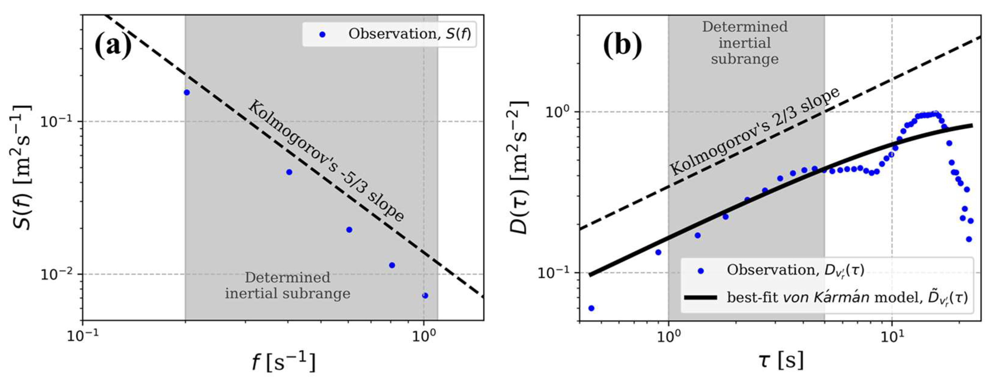For the estimation of $\mathrm{E}\mathrm{D}{\mathrm{R}}_{\mathrm{V}\mathrm{P},\mathrm{P}\mathrm{S}}$, the inertial subrange was chosen to be between 0.2 and 1.1 Hz, utilizing all available frequency bands. An example of the calculated PS is illustrated in Figure 4a.

3.2.2. Second-Order Structure Function Technique ($\mathrm{E}\mathrm{D}{\mathrm{R}}_{\mathrm{V}\mathrm{P},\mathrm{S}\mathrm{F}}$)

The estimation technique for $\mathrm{E}\mathrm{D}{\mathrm{R}}_{\mathrm{V}\mathrm{P},\mathrm{S}\mathrm{F}}$ is similar to that used for $\mathrm{E}\mathrm{D}{\mathrm{R}}_{\mathrm{S}\mathrm{o}\mathrm{n}\mathrm{i}\mathrm{c}}$. $w^{\prime }$ can be represented by the fluctuation of radial wind velocity $v_r^{\prime }$ in the VP scan. Thus, from Equation (9), we can obtain

$$ED{R}_{VP,SF}={\left({\displaystyle \frac{1}{U}}\right)}^{1/3}{\left[{\displaystyle \frac{\overline{D_{v_r^{\prime }}\left(\tau \right){\tau }^{-2/3}}}{C_1}}\right]}^{1/2}.$$

(14)

The inertial subrange used for the estimation spans 1 to 5 s, which is consistent with the estimation of $\mathrm{E}\mathrm{D}{\mathrm{R}}_{\mathrm{S}\mathrm{o}\mathrm{n}\mathrm{i}\mathrm{c}}$. An example of the calculated SF is provided in Figure 4b.

3.2.3. Variance Technique ($\mathrm{E}\mathrm{D}{\mathrm{R}}_{\mathrm{V}\mathrm{P},\mathrm{V}\mathrm{a}}$)

The technique for estimating EDR, which uses variance, was investigated by [7]. The underlying assumption is that the variance calculated from the observed radial velocity is primarily influenced by turbulence. As a result, the integral of PS can be expressed as equal to the variance of the radial velocity, represented mathematically as

$${\sigma }_{v_r}^2={\int }_{{\kappa }_0}^{{\kappa }_1}{F}_{22}\left(\kappa \right)d\kappa$$

(15)

$$=-{\displaystyle \frac{3}{2}}{C}_2{\epsilon }^{2/3}\left({\kappa }_1^{-2/3}-{\kappa }_0^{-2/3}\right)$$

(16)

$$={\displaystyle \frac{3}{2}}{C}_2{\left({\displaystyle \frac{\epsilon }{2\pi }}\right)}^{2/3 }\left(l_0^{2/3}-l_1^{2/3}\right).$$

(17)

The largest observable eddy length scale $l_0$(${\kappa }_0=2\pi /l_0$) is defined as $l_0=NU\psi$, where $N$ is the number of data points and $\psi$ is the dwell time. The smallest scale $l_1({\kappa }_1=2\pi /l_1)$ is defined as $l_1=U\psi$. Consequently, the EDR value is obtained with

$$ED{R}_{VP,Va}={\left(2\pi \right)}^{1/3}{\left({\displaystyle \frac{2}{3C_2}}\right)}^{1/2}{\sigma }_{v_r}{\left(l_0^{2/3}-l_1^{2/3}\right)}^{-1/2}.$$

(18)

3.2.4. SF Model Fitting Technique ($\mathrm{E}\mathrm{D}{\mathrm{R}}_{\mathrm{V}\mathrm{P},\mathrm{S}\mathrm{F}\left(\mathrm{f}\mathrm{i}\mathrm{t}\right)}$)

The EDR estimation technique, which uses an empirical turbulence model, was investigated by [9]. The $\mathrm{E}\mathrm{D}{\mathrm{R}}_{\mathrm{V}\mathrm{P},\mathrm{S}\mathrm{F}}$ is estimated directly from the calculated SF, while $\mathrm{E}\mathrm{D}{\mathrm{R}}_{\mathrm{V}\mathrm{P},\mathrm{S}\mathrm{F}\left(\mathrm{f}\mathrm{i}\mathrm{t}\right)}$ is estimated by fitting the SF with a turbulence model that has been empirically determined in prior studies. The empirical model for the SF is expressed as follows:

$${\tilde{D}}_{v_r^{\prime }}\left(s\right)=2{\sigma }_{v_r^{\prime }}^2\mathsf{\Lambda }\left({\displaystyle \frac{s}{l_{EI}}}\right)$$

(19)

where $\mathsf{\Lambda }$ is a universal function and $l_{EI}$ represents the outer scale of turbulence. For the von Kármán model [33], $\mathsf{\Lambda }$ is defined as

$$\Lambda \left(x\right)=1.0-0.593548 x^{1/3}{K}_{1/3}\left(x\right),$$

(20)

where $K_{1/3}$ is the modified Bessel function of order 1/3. By substituting $s=U\tau$ into Equation (19), the SF model in the time domain ${\tilde{D}}_{v_r^{\prime }}\left(\tau \right)$ can be obtained. Assuming that the right-hand sides of Equations (6) and (19) are equal, the EDR can be calculated as follows:

$$ED{R}_{VP,SF\left(fit\right)}={\left(0.933688{\displaystyle \frac{{\sigma }_{v_r^{\prime }}^3}{l_{EI}}}\right)}^{1/3}.$$

(21)

A weighted least-squares fit is employed in the fitting process. The parameters ${\sigma }_{v_r^{\prime }}$ and $l_{EI}$ are determined by minimizing the following weighted error:

$$J^2\left({\sigma }_{v_r^{\prime }},l_{EI}\right)=\sum _{k=1}^{N_t}{N}_I\left(k∆\tau \right){\left[D_{v_r^{\prime }}\left(k∆\tau \right)-{\tilde{D}}_{v_r^{\prime }}\left(\tau \right)\left(k∆\tau ,{\sigma }_{v_r^{\prime }},l_{EI}\right)\right]}^2$$

(22)

where $\mathsf{\Delta }\tau$ is the time interval change, which is equal to the dwell time, the smallest possible time interval between two points in a time series. $N_I$ is the number of data points used to calculate $D_{v_r^{\prime }}$ when $\tau =k∆\tau$, and $N_t$ is the maximum number of lags. Figure 4b demonstrates a successful fitting case where the best-fit von Kármán model was particularly effective and aligns with the observations within the inertial subrange. Please note that the discrepancies outside of the inertial subrange are expected due to the limitation in capturing physical processes at larger or smaller scales.

3.3. PPI Scanning Lidar-Based $ED{R}_{VAD}$

Mean wind profiles can be calculated using the VAD technique. The fluctuation component of wind velocity due to turbulence is determined by subtracting the mean wind component from the radial velocity. To compute the mean wind profiles, we employ the Singular Value Decomposition (SVD) approach, as detailed in reference [34].

The fluctuation component of wind velocity can be expressed as

$$v_r^{\prime }\left(\theta \right)=v_r\left(\theta \right)-\mathit{S}\left(\theta \right)\cdot 〈\mathit{v}〉,$$

(23)

where $\mathit{S}\left(\theta \right)=\{\sin \theta \cos \varphi ,\cos \theta \cos \varphi ,\sin \varphi \}$ is the unit vector along the probing beam and $〈\mathit{v}〉$ represents the mean wind vector estimated through sine wave least-squares fitting using SVD. An example of calculating $v_r^{\prime }$ is illustrated in Figure 5. The observed radial velocity was successfully fitted using SVD. The fitted velocity indicates that the wind speed at the time was ~11 m s⁻¹ and the wind direction was ~50°.

To ensure the reliability of the data, the coefficient of determination $R^2$ was used to evaluate the horizontal homogeneity of the wind field during the PPI scan. $R^2$ is defined as

$$R^2=1-\sum {\left(v_{r,i}-{\tilde{v}}_{r,i}\right)}^2/\sum {\left(v_{r,i}-{\overline{V}}_r\right)}^2,$$

(24)

where ${\tilde{v}}_{r,i}$ denotes the radial velocities calculated from the least-squares fit, while ${\overline{V}}_r$ denotes the average radial velocity. A higher $R^2$ value suggests a stronger correlation between the observed radial velocity and the fitted value, indicating that the atmosphere in the sensing area is more homogeneous. Data with $R^2$ values of 0.7 or greater were selected to measure turbulence-induced fluctuations while maintaining the quality of the mean wind field. Note that the threshold for $R^2$ in this study was not set as rigorously as in [34], as the focus is on turbulence.

The SF technique was used to estimate $\mathrm{E}\mathrm{D}{\mathrm{R}}_{\mathrm{V}\mathrm{A}\mathrm{D}}$. Equation (6) can be expressed for EDR as follows:

$$ED{R}_{VAD}={\left[{\displaystyle \frac{\overline{D_{v_r^{\prime }}\left(s\right)s^{-2/3}}}{C_2}}\right]}^{1/2}$$

(25)

where $s=r\cos \varphi \mathsf{\Delta }\theta$, with $\mathsf{\Delta }\theta$ representing the azimuth angle interval. The inertial subrange was selected to align with that used in $\mathrm{E}\mathrm{D}{\mathrm{R}}_{\mathrm{V}\mathrm{P}}$. Figure 6 illustrates the structure function $D_{v_r^{\prime }}\left(s\right)$, based on the VAD technique. To determine the inertial subrange, the same 1–5 s range used in estimating $\mathrm{E}\mathrm{D}{\mathrm{R}}_{\mathrm{S}\mathrm{o}\mathrm{n}\mathrm{i}\mathrm{c}}$ and $\mathrm{E}\mathrm{D}{\mathrm{R}}_{\mathrm{V}\mathrm{P},\mathrm{S}\mathrm{F}}$ was multiplied by $U$, resulting in the range of $U$–5$U$ m. In this study, if $s$ was within in the determined inertial subrange, the SF values in that region were averaged; otherwise, the values for the smallest $s$ were used.

4. Results

4.1. Evaluation of $ED{R}_{VAD}$ Using Sonic Anemometer

To evaluate the performance of $\mathrm{E}\mathrm{D}{\mathrm{R}}_{\mathrm{V}\mathrm{A}\mathrm{D}}$ in comparison to $\mathrm{E}\mathrm{D}{\mathrm{R}}_{\mathrm{S}\mathrm{o}\mathrm{n}\mathrm{i}\mathrm{c}}$ with respect to the temporal variations in turbulence intensity, Figure 7 presents the time series for both $\mathrm{E}\mathrm{D}{\mathrm{R}}_{\mathrm{S}\mathrm{o}\mathrm{n}\mathrm{i}\mathrm{c}}$ and $\mathrm{E}\mathrm{D}{\mathrm{R}}_{\mathrm{V}\mathrm{A}\mathrm{D}}$ at two altitudes (140 m and 300 m) across all elevation angles (20°, 30°, 45°, and 80°). Overall, the $\mathrm{E}\mathrm{D}{\mathrm{R}}_{\mathrm{V}\mathrm{A}\mathrm{D}}$ measurements across all elevation angles exhibited similar temporal variations to the $\mathrm{E}\mathrm{D}{\mathrm{R}}_{\mathrm{S}\mathrm{o}\mathrm{n}\mathrm{i}\mathrm{c}}$ measurements. As the elevation angle decreases, the estimated EDR generally becomes more similar to those from the sonic anemometer and better capture the variability. The $\mathrm{E}\mathrm{D}{\mathrm{R}}_{\mathrm{V}\mathrm{A}\mathrm{D}}$ measurement taken at the 80° scan in particular shows slightly lower values compared to the other elevation angles. We also observed typical diurnal variability of the PBL, especially on April 13, characterized by stronger turbulence during the day and weaker turbulence at night. There were also periods with less pronounced diurnal variability, such as on April 17, which were influenced by external factors from low-pressure system passages.

Figure 8 presents density scatter plots and performance metrics based on Figure 7 data to evaluate the performance of $\mathrm{E}\mathrm{D}{\mathrm{R}}_{\mathrm{V}\mathrm{A}\mathrm{D}}$ at various elevation angles. The $\mathrm{E}\mathrm{D}{\mathrm{R}}_{\mathrm{V}\mathrm{A}\mathrm{D}}$ demonstrated a correlation coefficient (CORR) greater than 0.5 for all elevation angles at both altitudes, indicating an overall agreement with the sonic anemometer. A negative bias was generally observed. This discrepancy is likely due to the difference in sensing volumes between the two instruments. The CSAT3 sonic anemometer has a 10 cm spacing between its ultrasonic sensor pair and a temporal resolution of 0.05 s. In contrast, the Windex lidar has a gate length of 40 m and a time to observe a single ray of 0.6 s. The lidar observes a significantly larger sensing volume than the sonic anemometer, which may contribute to smoothing out some fluctuations caused by turbulence.

The performance metrics reveal that $\mathrm{E}\mathrm{D}{\mathrm{R}}_{\mathrm{V}\mathrm{A}\mathrm{D}}$ achieved better performance at lower elevation angles compared to higher ones. The CORR improved as the elevation angle decreased, accompanied by a reduction in standard deviation (STD). At the elevation angle of 80°, a significant bias of −0.45 and −0.47 ($\mathrm{l}\mathrm{o}{\mathrm{g}}_{10}\mathrm{E}\mathrm{D}\mathrm{R}$) was noted at altitudes of 140 m and 300 m, respectively. Higher EDR values exhibited a greater tendency towards underestimation. The variation in bias at elevation angles of 45°, 30°, and 20°—with the exception of 80°—suggests that EDR values tend to decrease (they are underestimated) as the elevation angle decreases at the altitude of 140 m. Conversely, at a 300 m altitude, the underestimation of EDR gradually decreased with lowering elevation angles.

4.2. Intercomparison of $ED{R}_{VP}$ Estimation Techniques

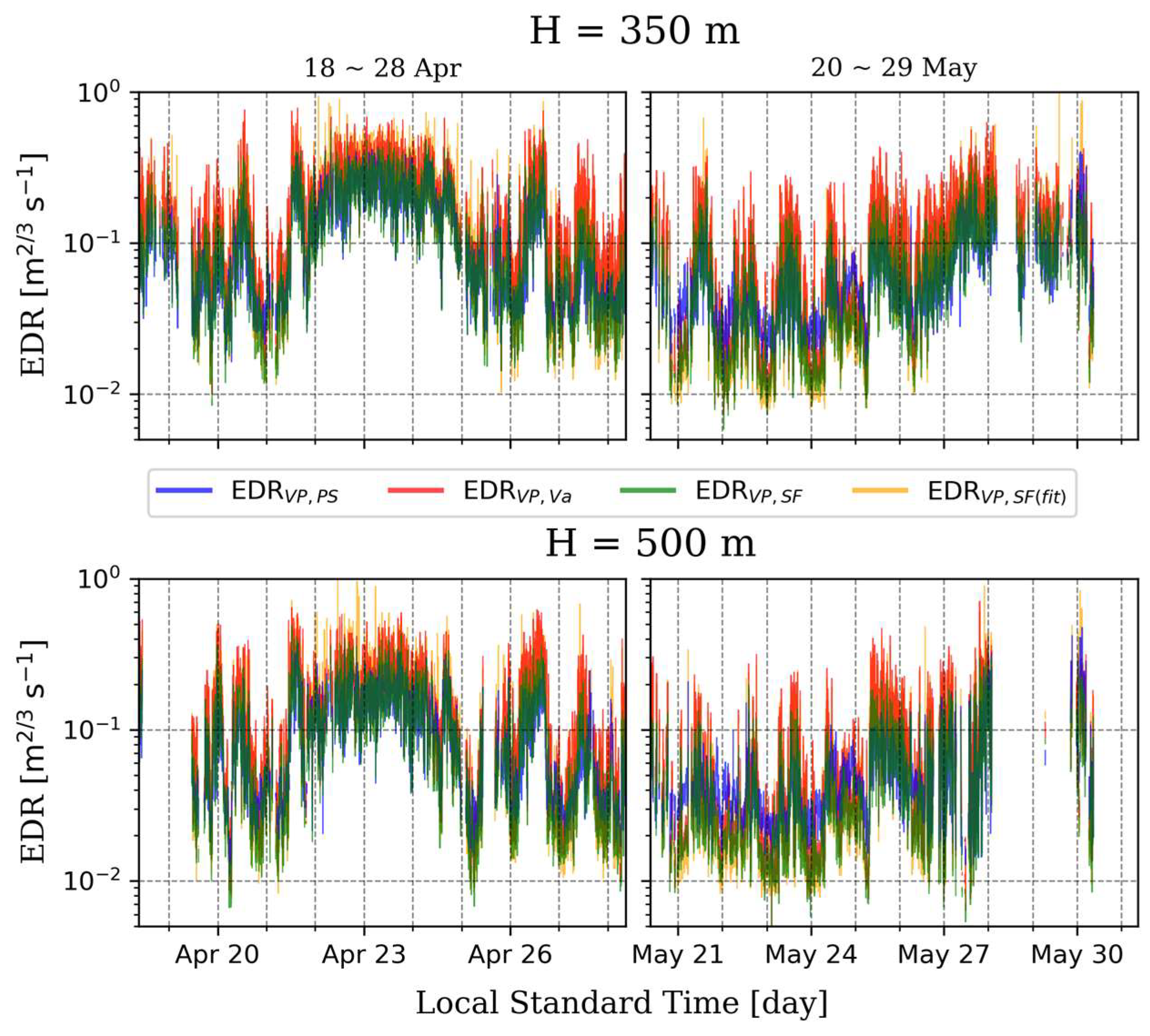
Figure 9 presents the time series of EDR at two altitudes, calculated using four different techniques from the VP scan during the Jeju experiment. The four techniques demonstrate a consistent trend over time, exhibiting nearly identical diurnal variation in EDR values, particularly from 21 May to 24 May. However, $\mathrm{E}\mathrm{D}{\mathrm{R}}_{\mathrm{V}\mathrm{P},\mathrm{V}\mathrm{a}}$ is notably higher than the values estimated by the other methods. $\mathrm{E}\mathrm{D}{\mathrm{R}}_{\mathrm{V}\mathrm{P},\mathrm{P}\mathrm{S}}$ shows higher values at low EDR levels compared to other techniques. $\mathrm{E}\mathrm{D}{\mathrm{R}}_{\mathrm{V}\mathrm{P},\mathrm{S}\mathrm{F}\left(\mathrm{f}\mathrm{i}\mathrm{t}\right)}$ exhibits a few outliers.

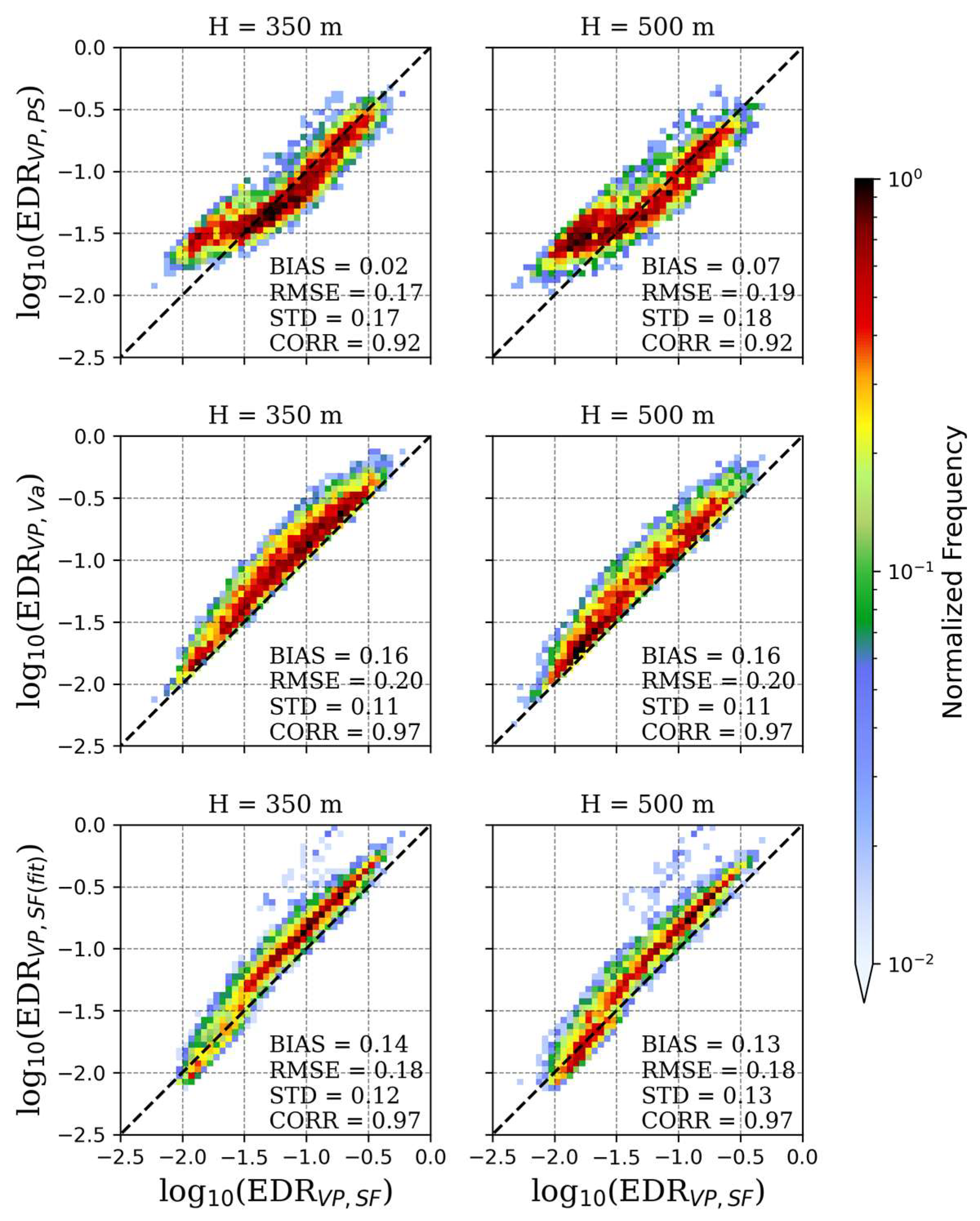
For quantitative comparison, the other techniques were evaluated against $\mathrm{E}\mathrm{D}{\mathrm{R}}_{\mathrm{V}\mathrm{P},\mathrm{S}\mathrm{F}}$ using density scatter plots (see Figure 10). The $\mathrm{E}\mathrm{D}{\mathrm{R}}_{\mathrm{V}\mathrm{P},\mathrm{P}\mathrm{S}}$ technique showed the least bias at both altitudes compared to the other methods. This minimal bias likely arises because both $\mathrm{E}\mathrm{D}{\mathrm{R}}_{\mathrm{V}\mathrm{P},\mathrm{S}\mathrm{F}}$ and $\mathrm{E}\mathrm{D}{\mathrm{R}}_{\mathrm{V}\mathrm{P},\mathrm{P}\mathrm{S}}$ techniques utilize wavelet analysis and use the same range of inertial subranges. However, $\mathrm{E}\mathrm{D}{\mathrm{R}}_{\mathrm{V}\mathrm{P},\mathrm{P}\mathrm{S}}$ tends to be larger when $\mathrm{E}\mathrm{D}{\mathrm{R}}_{\mathrm{V}\mathrm{P},\mathrm{S}\mathrm{F}}$ falls below approximately ${10}^{-1.5}(0.03 {\mathrm{m}}^{2/3} {\mathrm{s}}^{-1})$, and this discrepancy is more pronounced at higher altitudes of 500 m compared to 350 m. This trend was also noted by [29], who suggested that the magnitude of FFT noise becomes comparable to the observed values when EDR is relatively low. In comparing the two altitudes of $\mathrm{E}\mathrm{D}{\mathrm{R}}_{\mathrm{V}\mathrm{P},\mathrm{P}\mathrm{S}}$, a greater incidence of weak turbulence is observed at 500 m than at 350 m, leading to a higher frequency of overestimation at these small EDR values. As a result, the bias and root mean squared error (RMSE) are worse at 500 m compared to 350 m.

The CORR of $\mathrm{E}\mathrm{D}{\mathrm{R}}_{\mathrm{V}\mathrm{P},\mathrm{V}\mathrm{a}}$ is 0.97 at both altitudes, indicating a strong relationship with $\mathrm{E}\mathrm{D}{\mathrm{R}}_{\mathrm{V}\mathrm{P},\mathrm{S}\mathrm{F}}$. However, it has the highest bias (0.16) among all of the techniques. The scatterplot illustrates that $\mathrm{E}\mathrm{D}{\mathrm{R}}_{\mathrm{V}\mathrm{P},\mathrm{V}\mathrm{a}}$ shows a more significant difference at higher EDR values compared to lower ones.

This discrepancy may arise from the assumption made using the $\mathrm{E}\mathrm{D}{\mathrm{R}}_{\mathrm{V}\mathrm{P},\mathrm{V}\mathrm{a}}$ estimation technique, which considers the entire sampling time to be an inertial subrange. Uncertainty increases when the actual inertial subrange deviates from this assumption. In conditions of strong turbulence, larger turbulent eddies are formed, suggesting that a longer sampling time is beneficial for effectively observing them. Conversely, weak turbulence produces smaller eddies, which are better captured with a shorter sampling time. If the sampling time is shorter than the actual inertial subrange of the measured events, the influence of instrumental noise may become more significant, leading to an overestimation of the results. On the other hand, if the sampling time is longer, the EDR may be underestimated, as it would be more influenced by large-scale processes rather than by turbulence. To tackle this issue, [12] proposed a method for calculating $\mathrm{E}\mathrm{D}{\mathrm{R}}_{\mathrm{V}\mathrm{P},\mathrm{V}\mathrm{a}}$ by adjusting the sampling time based on atmospheric instability. Their findings suggest that a 27 s sampling time is appropriate for stable conditions, while an 82 s sampling time is more suitable for unstable conditions. In this study, a 30 s sampling time was utilized, which is adequate for observing small turbulent eddies under stable atmospheric conditions. However, this sampling time has limitations when it comes to detecting larger turbulent eddies in unstable atmospheres, leading to an overestimation of the $\mathrm{E}\mathrm{D}{\mathrm{R}}_{\mathrm{V}\mathrm{P},\mathrm{V}\mathrm{a}}$.

The CORR between $\mathrm{E}\mathrm{D}{\mathrm{R}}_{\mathrm{V}\mathrm{P},\mathrm{S}\mathrm{F}\left(\mathrm{f}\mathrm{i}\mathrm{t}\right)}$ and $\mathrm{E}\mathrm{D}{\mathrm{R}}_{\mathrm{V}\mathrm{P},\mathrm{S}\mathrm{F}}$ was found to be 0.97 at both altitudes. However, the bias in the estimates was 0.14 at 350 m and 0.13 at 500 m, indicating that the estimates of $\mathrm{E}\mathrm{D}{\mathrm{R}}_{\mathrm{V}\mathrm{P},\mathrm{S}\mathrm{F}\left(\mathrm{f}\mathrm{i}\mathrm{t}\right)}$ were generally greater than those from $\mathrm{E}\mathrm{D}{\mathrm{R}}_{\mathrm{V}\mathrm{P},\mathrm{S}\mathrm{F}}$. Because $\mathrm{E}\mathrm{D}{\mathrm{R}}_{\mathrm{V}\mathrm{P},\mathrm{S}\mathrm{F}\left(\mathrm{f}\mathrm{i}\mathrm{t}\right)}$ heavily relies on the accuracy of the fitting process, we conducted an additional analysis to investigate the characteristics of cases that did not fit properly. 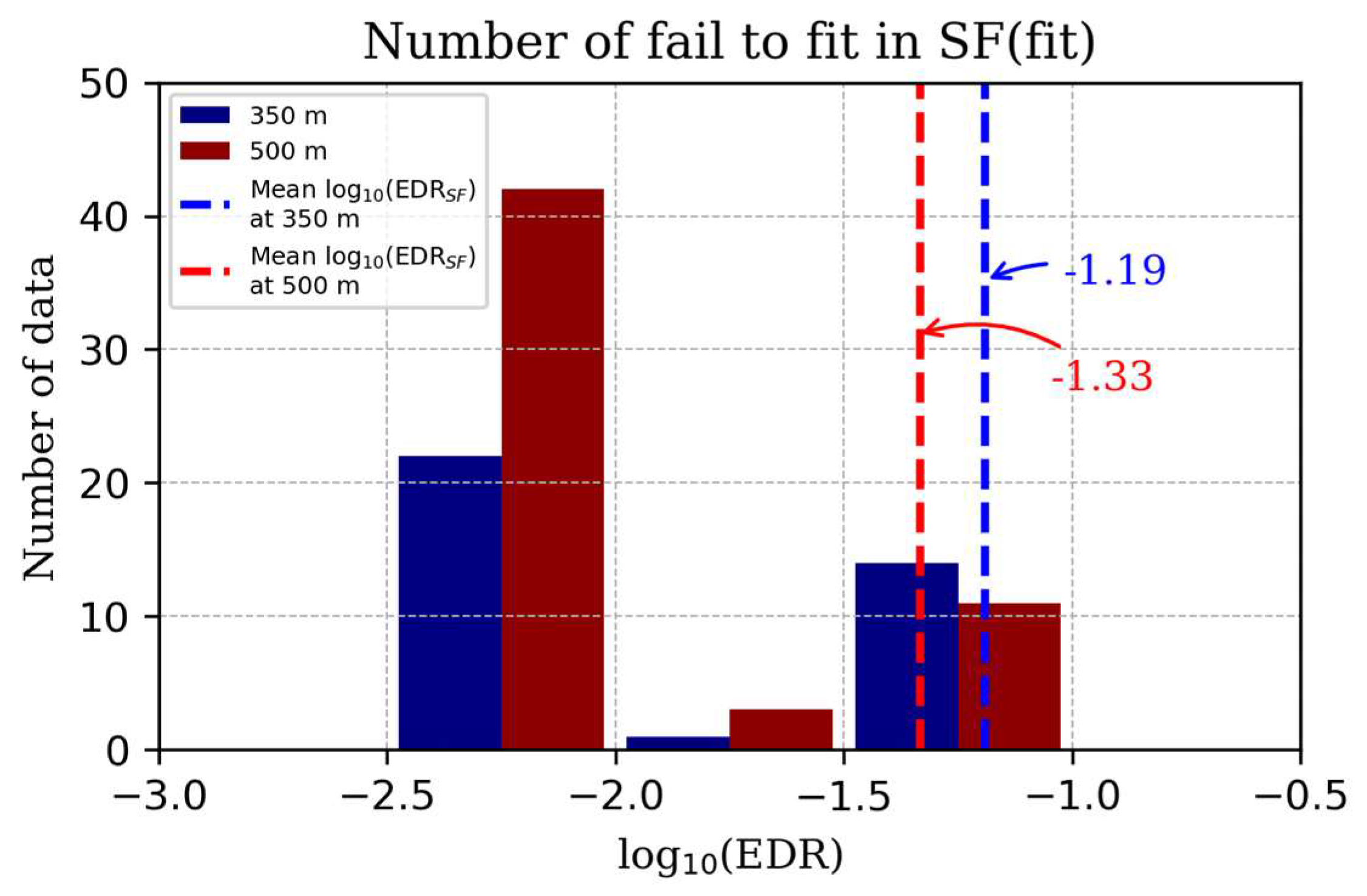Figure 11 presents a histogram that shows the number of cases that failed to fit during the estimation of $\mathrm{E}\mathrm{D}{\mathrm{R}}_{\mathrm{V}\mathrm{P},\mathrm{S}\mathrm{F}\left(\mathrm{f}\mathrm{i}\mathrm{t}\right)}$, categorized by the magnitude of $\mathrm{E}\mathrm{D}{\mathrm{R}}_{\mathrm{V}\mathrm{P},\mathrm{S}\mathrm{F}}$. The failure in fitting is defined as a case where the optimization process fails to minimize the cost function (Equation (22)). There were 56 failed cases at 500 m and 37 failed cases at 350 m, resulting in success rates of 97.2% and 98.2%, respectively, out of approximately 2000 cases. Most of the failed fits occurred when the turbulence intensity was relatively low compared to the average. Although the number of cases with fit failures is relatively small, these failures in weak turbulence may contribute to the observed positive bias in $\mathrm{E}\mathrm{D}{\mathrm{R}}_{\mathrm{V}\mathrm{P},\mathrm{S}\mathrm{F}\left(\mathrm{f}\mathrm{i}\mathrm{t}\right)}$.

By closely examining $\mathrm{E}\mathrm{D}{\mathrm{R}}_{\mathrm{V}\mathrm{P},\mathrm{V}\mathrm{a}}$ and $\mathrm{E}\mathrm{D}{\mathrm{R}}_{\mathrm{V}\mathrm{P},\mathrm{S}\mathrm{F}\left(\mathrm{f}\mathrm{i}\mathrm{t}\right)}$, which exhibit similar performance, several insights can be drawn. First, in conditions where the bias unknown, $\mathrm{E}\mathrm{D}{\mathrm{R}}_{\mathrm{V}\mathrm{P},\mathrm{S}\mathrm{F}\left(\mathrm{f}\mathrm{i}\mathrm{t}\right)}$ may be a more recommended choice due to its smaller bias and RMSE. Second, if the bias is known, $\mathrm{E}\mathrm{D}{\mathrm{R}}_{\mathrm{V}\mathrm{P},\mathrm{V}\mathrm{a}}$ may generally be the better performing option because it has a smaller standard deviation and the systematic bias can be corrected. Lastly, for practical reasons, such as aviation warnings, where the focus is on cases of strong turbulence, $\mathrm{E}\mathrm{D}{\mathrm{R}}_{\mathrm{V}\mathrm{P},\mathrm{S}\mathrm{F}\left(\mathrm{f}\mathrm{i}\mathrm{t}\right)}$ would be preferable due to its more concentrated scatter for EDR > 10^−1.5. Conversely, for research purposes or situations requiring consistent performance across the full range of turbulence intensities, $\mathrm{E}\mathrm{D}{\mathrm{R}}_{\mathrm{V}\mathrm{P},\mathrm{V}\mathrm{a}}$ would be more advantageous due to its lower dependency of performance on EDR intensity.

4.3. Comparison of $ED{R}_{VAD}$ and $ED{R}_{VP,SF}$

Section 4.2 involved an intercomparison of $\mathrm{E}\mathrm{D}{\mathrm{R}}_{\mathrm{V}\mathrm{P}}$ techniques; however, absolute validation was lacking. To address this limitation, the present section evaluates whether the $\mathrm{E}\mathrm{D}{\mathrm{R}}_{\mathrm{V}\mathrm{P}}$ (specifically, the $\mathrm{E}\mathrm{D}{\mathrm{R}}_{\mathrm{V}\mathrm{P},\mathrm{S}\mathrm{F}}$) exhibits significant bias in its absolute estimation when compared with $\mathrm{E}\mathrm{D}{\mathrm{R}}_{\mathrm{V}\mathrm{A}\mathrm{D}}$, which has already been validated against the sonic anemometer in Section 4.1. This section also examines their characteristics in relation to altitude. 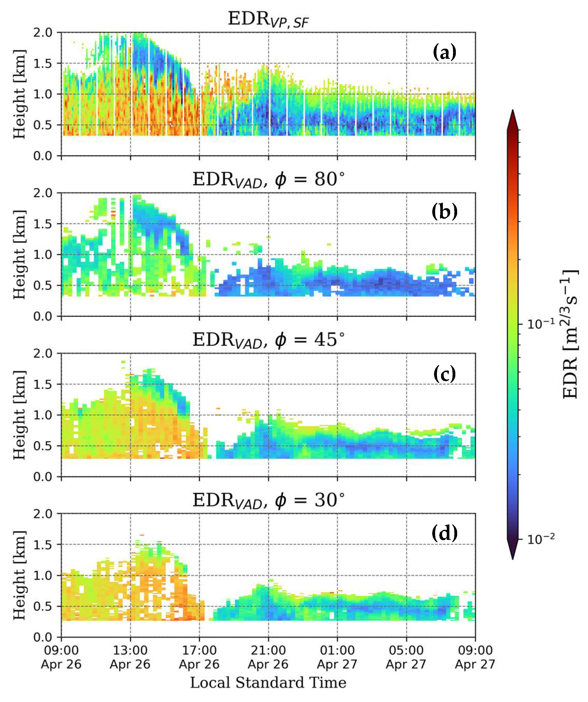Figure 12 presents a time–height plot of $\mathrm{E}\mathrm{D}{\mathrm{R}}_{\mathrm{V}\mathrm{P},\mathrm{S}\mathrm{F}}$ and $\mathrm{E}\mathrm{D}{\mathrm{R}}_{\mathrm{V}\mathrm{A}\mathrm{D}}$ at various elevation angles over a day. The analysis indicates a noticeable variation in turbulence intensity, with both $\mathrm{E}\mathrm{D}{\mathrm{R}}_{\mathrm{V}\mathrm{P},\mathrm{S}\mathrm{F}}$ and $\mathrm{E}\mathrm{D}{\mathrm{R}}_{\mathrm{V}\mathrm{A}\mathrm{D}}$ yielding similar spatial patterns. Both methods effectively represented the strong turbulence observed until 17:00, followed by a weaker turbulence after that. Upon examining the differences in $\mathrm{E}\mathrm{D}{\mathrm{R}}_{\mathrm{V}\mathrm{A}\mathrm{D}}$ in relation to the elevation angle, it was observed that higher elevation angles correspond to a higher maximum observable altitude. In contrast, lower elevation angles result in a lower maximum observable altitude. Additionally, the values of $\mathrm{E}\mathrm{D}{\mathrm{R}}_{\mathrm{V}\mathrm{A}\mathrm{D}}$ tended to increase and became more comparable to $\mathrm{E}\mathrm{D}{\mathrm{R}}_{\mathrm{V}\mathrm{P},\mathrm{S}\mathrm{F}}$ as the elevation angle decreased.

Figure 13 demonstrates density scatter plots comparing $\mathrm{E}\mathrm{D}{\mathrm{R}}_{\mathrm{V}\mathrm{P},\mathrm{S}\mathrm{F}}$ and $\mathrm{E}\mathrm{D}{\mathrm{R}}_{\mathrm{V}\mathrm{A}\mathrm{D}}$ at two altitudes (350 m and 500 m) throughout the entire Jeju experiment period, along with performance metrics. The results show that the $\mathrm{E}\mathrm{D}{\mathrm{R}}_{\mathrm{V}\mathrm{P},\mathrm{S}\mathrm{F}}$ and $\mathrm{E}\mathrm{D}{\mathrm{R}}_{\mathrm{V}\mathrm{A}\mathrm{D}}$ values are comparable, exhibiting a high CORR above 0.8, with only a slight bias at both altitudes and across all elevation angles. The observed bias indicates that the $\mathrm{E}\mathrm{D}{\mathrm{R}}_{\mathrm{V}\mathrm{A}\mathrm{D}}$ value tends to increase as the elevation angle decreases, a trend that is consistent with the previous comparison with the sonic anemometer at 300 m height. At both altitudes, $\mathrm{E}\mathrm{D}{\mathrm{R}}_{\mathrm{V}\mathrm{A}\mathrm{D}}$ with 80° scans showed the greatest bias and uncertainties, while 45° showed the best performance in comparison to the other elevation angles.

Figure 14 illustrates the performance metrics of $\mathrm{E}\mathrm{D}{\mathrm{R}}_{\mathrm{V}\mathrm{A}\mathrm{D}}$ as a function of altitude. The performance metrics were calculated under the assumption that $\mathrm{E}\mathrm{D}{\mathrm{R}}_{\mathrm{V}\mathrm{P},\mathrm{S}\mathrm{F}}$ represents the true value. To ensure the reliability of the analysis, altitudes with fewer than 50 data points were excluded. The number of observed data points indicates that the maximum observable altitude depends on the elevation angle; higher elevation angles allow for higher maximum observable altitudes. The bias tends to increase positively as the elevation angle decreases. Lower elevation angles are characterized by a greater rate of increase with altitude. These characteristics are also evident in the RMSE. At the elevation angle of 80°, RMSE shows a slight decrease with increasing altitude. However, at the other two angles, RMSE increases with altitude, with the most significant rate of increase observed at the lowest elevation angle. The STD is similar across all elevation angles, remaining below 0.3 (${\log }_{10}\mathrm{E}\mathrm{D}\mathrm{R}$). At most altitudes, the elevation angle of 45° exhibits the smallest STD. At the elevation angle of 30°, the CORR is lower than at other angles, while at 45°, it is generally the highest.

In summary, the elevation angle of 80° would be beneficial for measuring the EDR at high altitudes; however, it would be less precise at low altitudes compared to other elevation angles. At the elevation angle of 45°, the accuracy is the highest at low altitudes, but the bias increases as altitude increases. For the EDR estimation above approximately 600 m, where the RMSE of the 80° and 45° elevation angles intersects, the 80° angle would be optimal. Conversely, for the EDR estimation below this intersection point, the 45° angle is preferred. The accuracy of the 30° elevation angle decreases significantly with increasing altitude compared to other elevation angles, likely due to the extensive horizontal distance of the lidar beam at higher altitudes. This greater horizontal distance challenges the assumption of homogeneity in wind characteristics at equal distances from the lidar, leading to greater uncertainties.

5. Discussion

In Section 4.1, the $\mathrm{E}\mathrm{D}{\mathrm{R}}_{\mathrm{V}\mathrm{A}\mathrm{D}}$ estimations taken at the 80° elevation angle exhibited the poorest performance compared to estimations at other angles. This discrepancy can be attributed to the slower scan rate at 80° during the BMO field experiment. According to [35], if the tangential scan speed along the boundary of the scanning circle is significantly higher than the mean horizontal wind speed ($U$), the transfer of turbulent inhomogeneities by the mean flow can be considered negligible. During the BMO field experiment, the scan rate at the 80° elevation angle was 5° s⁻¹, which is slower than the 10° s⁻¹ rate at other angles. At 140 m and 300 m altitudes, the tangential speeds at the 80° elevation angle were 2.1 m s⁻¹ and 4.5 m s⁻¹, respectively. In contrast, the mean $U$ measured using the sonic anemometer during the entire BMO field experiment was 3.5 m s⁻¹ at 140 m and 4.0 m s⁻¹ at 300 m. At both altitudes, the tangential speeds were comparable to or below $U$. Consequently, the transfer of turbulent inhomogeneities by the mean flow at the 80° elevation angle may contribute to the uncertainties in $\mathrm{E}\mathrm{D}{\mathrm{R}}_{\mathrm{V}\mathrm{A}\mathrm{D}}$ estimation.

Additionally, the limited PPI scanning area relative to the inertial range may be the reason for these discrepancies. Ref. [36] indicated that the magnitude of error increases when the radius of the PPI scanning circle is comparable to or smaller than that of the inertial subrange. In this study, the scanning circle for the 80° PPI scan was significantly smaller than those for other elevation angles, likely contributing to the pronounced negative bias. Figure 14 demonstrates that the $\mathrm{E}\mathrm{D}{\mathrm{R}}_{\mathrm{V}\mathrm{A}\mathrm{D}}$ with the 80° scan shows a negative bias at low altitudes, but this bias diminishes as altitude increases. This pattern suggests that the scanning circle’s radius at the 80° elevation angle was smaller than or similar to the inertial subrange at lower altitudes, resulting in the observed worse (negative) bias, and vice versa at higher altitudes.

The negative bias was observed at all elevation angles when validating $\mathrm{E}\mathrm{D}{\mathrm{R}}_{\mathrm{V}\mathrm{A}\mathrm{D}}$ using the sonic anemometer. This bias can be attributed to the differences in sampling volumes between lidar and sonic anemometers. Ref. [18] introduced a technique that employs the transfer function of a low-frequency filter to account for the volume-averaging effect in lidar measurements. By applying this method, a study by [20] demonstrated that the underestimation caused by the sampling volume can be significantly reduced. The application of such techniques is expected to enhance performance, highlighting the need for further research to evaluate their effectiveness.

In the Jeju field experiment, there is a clear trend showing that the value of $\mathrm{E}\mathrm{D}{\mathrm{R}}_{\mathrm{V}\mathrm{A}\mathrm{D}}$ increases as the elevation angle decreases. Similarly, in the BMO field experiment, a noticeable increase in $\mathrm{E}\mathrm{D}{\mathrm{R}}_{\mathrm{V}\mathrm{A}\mathrm{D}}$ with lower elevation angles is observed at an altitude of 300 m, although this trend is not present at 140 m. This pattern of $\mathrm{E}\mathrm{D}{\mathrm{R}}_{\mathrm{V}\mathrm{A}\mathrm{D}}$ increasing with decreasing elevation angle may be related to the fluctuations in radial velocity $v_r\prime$. If turbulence were isotropic in three dimensions and the mean flow component could be entirely separated from the radial velocity, we would expect the observed fluctuations to exhibit similar values. However, in practice, fully separating the mean flow component in lidar measurements is challenging due to the inherent limitations in the velocity resolution of the lidar and the accuracy of the VAD fitting. It is possible that $v_r\prime$ still contains the mean flow component, which, ideally, should be excluded. Generally, in the atmosphere, the horizontal component of wind velocity is greater than the vertical component. This horizontal component tends to dominate at lower elevation angles during radial velocity measurements, likely explaining the more significant values of $v_r\prime$ observed at these angles.

The lidar observation data from BMO utilized a dwell time of 0.6 s. In comparison, the lidar observation data from Jeju employed different dwell times: 0.25 s for PPI scans and 0.45 s for VP scans (see Table 2). This variation in dwell times results in different sampling rates, which may impact the characterization of turbulence.

The various error sources mentioned can impact EDR estimation, making it challenging to determine which one has the greatest influence based on the findings of this study. Conducting further research on error sources could enhance the accuracy of EDR estimation techniques. Furthermore, this study did not directly compare the sonic anemometer with $\mathrm{E}\mathrm{D}{\mathrm{R}}_{\mathrm{V}\mathrm{P}}$ due to data limitations; therefore, additional verification of $\mathrm{E}\mathrm{D}{\mathrm{R}}_{\mathrm{V}\mathrm{P}}$ estimation techniques is helpful.

6. Conclusions

This study assessed the accuracy of various estimation techniques for EDR using Doppler lidar. The $\mathrm{E}\mathrm{D}{\mathrm{R}}_{\mathrm{V}\mathrm{A}\mathrm{D}}$ estimation technique, based on PPI scans, was validated with data collected from sonic anemometers on the 300 m tall meteorological tower during the BMO field experiment. Four estimation techniques based on VP scans were intercompared, and their characteristics were analyzed. Finally, the accuracy of the $\mathrm{E}\mathrm{D}{\mathrm{R}}_{\mathrm{V}\mathrm{A}\mathrm{D}}$ technique was evaluated against $\mathrm{E}\mathrm{D}{\mathrm{R}}_{\mathrm{V}\mathrm{P},\mathrm{S}\mathrm{F}}$ at different altitudes.

The validation of $\mathrm{E}\mathrm{D}{\mathrm{R}}_{\mathrm{V}\mathrm{A}\mathrm{D}}$ indicated that it effectively captured the variations in turbulence intensity, including diurnal variations, demonstrating its ability to replicate the key characteristics observed in $\mathrm{E}\mathrm{D}{\mathrm{R}}_{\mathrm{S}\mathrm{o}\mathrm{n}\mathrm{i}\mathrm{c}}$, with the CORR exceeding 0.5 for all elevation angles. $\mathrm{E}\mathrm{D}{\mathrm{R}}_{\mathrm{V}\mathrm{A}\mathrm{D}}$ showed improved accuracy at lower elevation angles; however, it slightly underestimated the values at the 80° angle compared to other angles.

The intercomparison of the four estimation techniques for $\mathrm{E}\mathrm{D}{\mathrm{R}}_{\mathrm{V}\mathrm{P}}$ indicated that they all yielded highly similar values. Among these, $\mathrm{E}\mathrm{D}{\mathrm{R}}_{\mathrm{V}\mathrm{P},\mathrm{P}\mathrm{S}}$ showed values most similar to those of $\mathrm{E}\mathrm{D}{\mathrm{R}}_{\mathrm{V}\mathrm{P},\mathrm{S}\mathrm{F}}$, indicating the smallest bias. However, $\mathrm{E}\mathrm{D}{\mathrm{R}}_{\mathrm{V}\mathrm{P},\mathrm{P}\mathrm{S}}$ tended to overestimate under conditions of relatively weak turbulence, likely due to noise from the FFT analysis. The results for $\mathrm{E}\mathrm{D}{\mathrm{R}}_{\mathrm{V}\mathrm{P},\mathrm{V}\mathrm{a}}$ and $\mathrm{E}\mathrm{D}{\mathrm{R}}_{\mathrm{V}\mathrm{P},\mathrm{S}\mathrm{F}\left(\mathrm{f}\mathrm{i}\mathrm{t}\right)}$ demonstrated a strong correlation with $\mathrm{E}\mathrm{D}{\mathrm{R}}_{\mathrm{V}\mathrm{P},\mathrm{S}\mathrm{F}}$, with a CORR of 0.97. Notably, $\mathrm{E}\mathrm{D}{\mathrm{R}}_{\mathrm{V}\mathrm{P},\mathrm{V}\mathrm{a}}$ had the highest value among all techniques, likely due to the selection of the sampling time used for variance calculation, which may be suboptimal and has a strong impact on its performance. If the sampling time does not correspond to the inertial subrange of the actual atmospheric turbulence, this can lead to uncertainties in EDR estimation. Conversely, $\mathrm{E}\mathrm{D}{\mathrm{R}}_{\mathrm{V}\mathrm{P},\mathrm{S}\mathrm{F}\left(\mathrm{f}\mathrm{i}\mathrm{t}\right)}$ depends heavily on the accuracy of the fitting process and is particularly prone to failure under low turbulence conditions. When high temporal resolution observations are available, it is advisable to use wavelet analysis techniques, such as $\mathrm{E}\mathrm{D}{\mathrm{R}}_{\mathrm{V}\mathrm{P},\mathrm{P}\mathrm{S}}$ and $\mathrm{E}\mathrm{D}{\mathrm{R}}_{\mathrm{V}\mathrm{P},\mathrm{S}\mathrm{F}}$, for greater accuracy. Conversely, when only relatively low temporal resolution observations are accessible, $\mathrm{E}\mathrm{D}{\mathrm{R}}_{\mathrm{V}\mathrm{P},\mathrm{V}\mathrm{a}}$ can be advantageous as it does not require wavelet analysis. $\mathrm{E}\mathrm{D}{\mathrm{R}}_{\mathrm{V}\mathrm{P},\mathrm{S}\mathrm{F}\left(\mathrm{f}\mathrm{i}\mathrm{t}\right)}$ can allow for correction through fitting even with limited data.

The accuracy of $\mathrm{E}\mathrm{D}{\mathrm{R}}_{\mathrm{V}\mathrm{A}\mathrm{D}}$ based on the PPI scan was evaluated against $\mathrm{E}\mathrm{D}{\mathrm{R}}_{\mathrm{V}\mathrm{P},\mathrm{S}\mathrm{F}}$. It was observed that the maximum altitude at which $\mathrm{E}\mathrm{D}{\mathrm{R}}_{\mathrm{V}\mathrm{A}\mathrm{D}}$ could be reliably measured increased with higher elevation angles and decreased with lower angles. Additionally, $\mathrm{E}\mathrm{D}{\mathrm{R}}_{\mathrm{V}\mathrm{A}\mathrm{D}}$ exhibited larger values at lower elevation angles, along with a greater rate of increase with altitude. The results emphasize the importance of carefully selecting the elevation angle based on altitude; using a 45° elevation angle yields higher accuracy at lower altitudes, while the 80° elevation angle is more accurate at higher altitudes.

The advantages and disadvantages of each technique described in the conclusion are summarized in

Table 3. Advantages and disadvantages of each estimation technique.

Techniques		Strength	Weakness
$\mathrm{E}\mathrm{D}{\mathrm{R}}_{\mathrm{V}\mathrm{A}\mathrm{D}}$	Low angle	- High vertical resolution - High accuracy at the lower altitude	- Limitations when observing the upper altitude - Possibility of beam blocking by terrain
	High angle	- High accuracy at the upper altitude	- Low accuracy at the lower altitude - Low vertical resolution
$\mathrm{E}\mathrm{D}{\mathrm{R}}_{\mathrm{V}\mathrm{P}}$	PS	- Inertial subrange can be adjusted	- High sampling frequency is required - Overestimation for weak turbulence
	SF	- Inertial subrange can be adjusted	- High sampling frequency is required
	Va	- Wavelet analysis is not required	- Predetermined inertial subrange by sampling time
	SF(fit)	- Good performance for strong turbulence	- Potential for fitting failure for weak turbulence

.