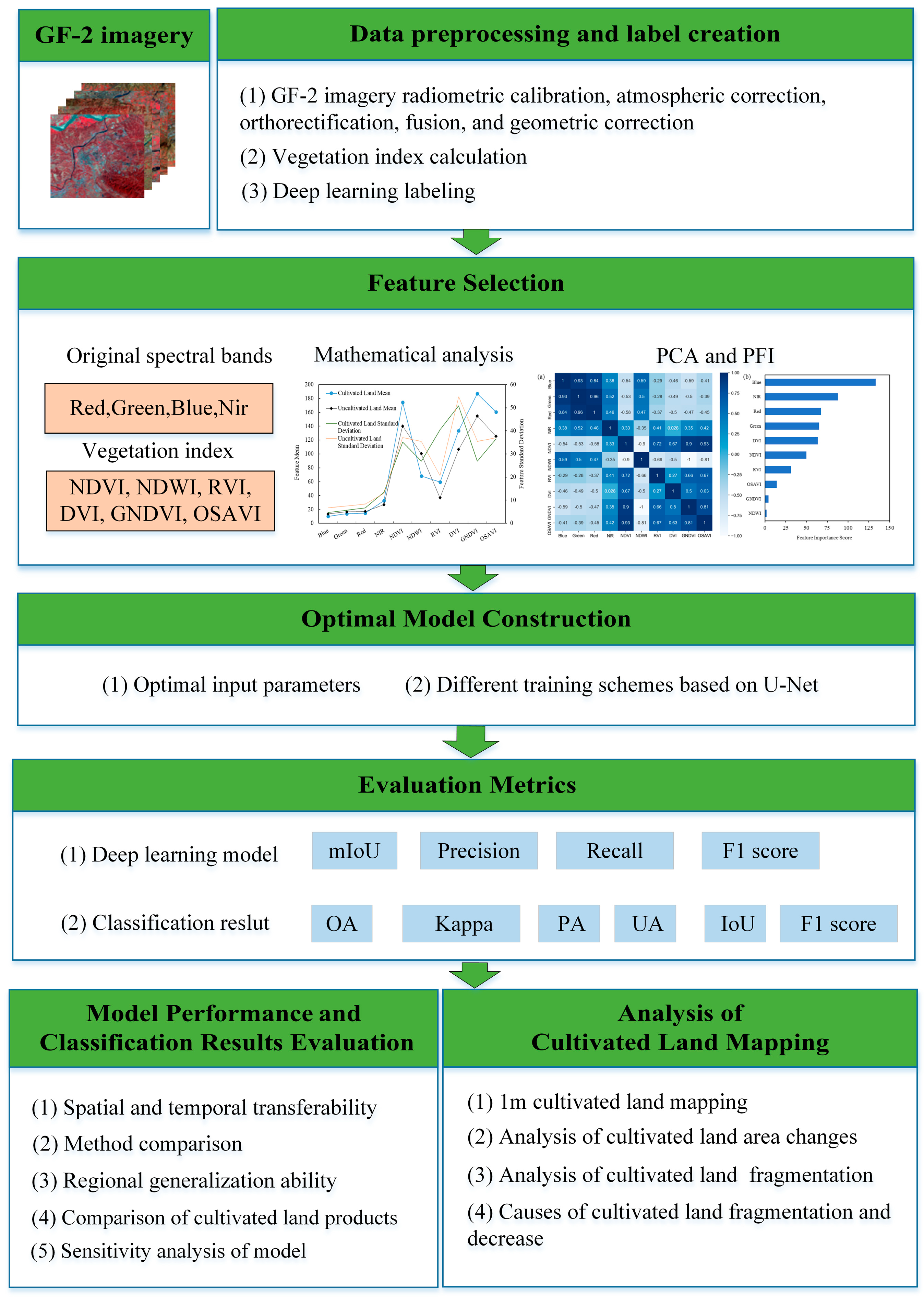
Figure 1.
The overall workflow of this study.
Figure 1.
The overall workflow of this study.
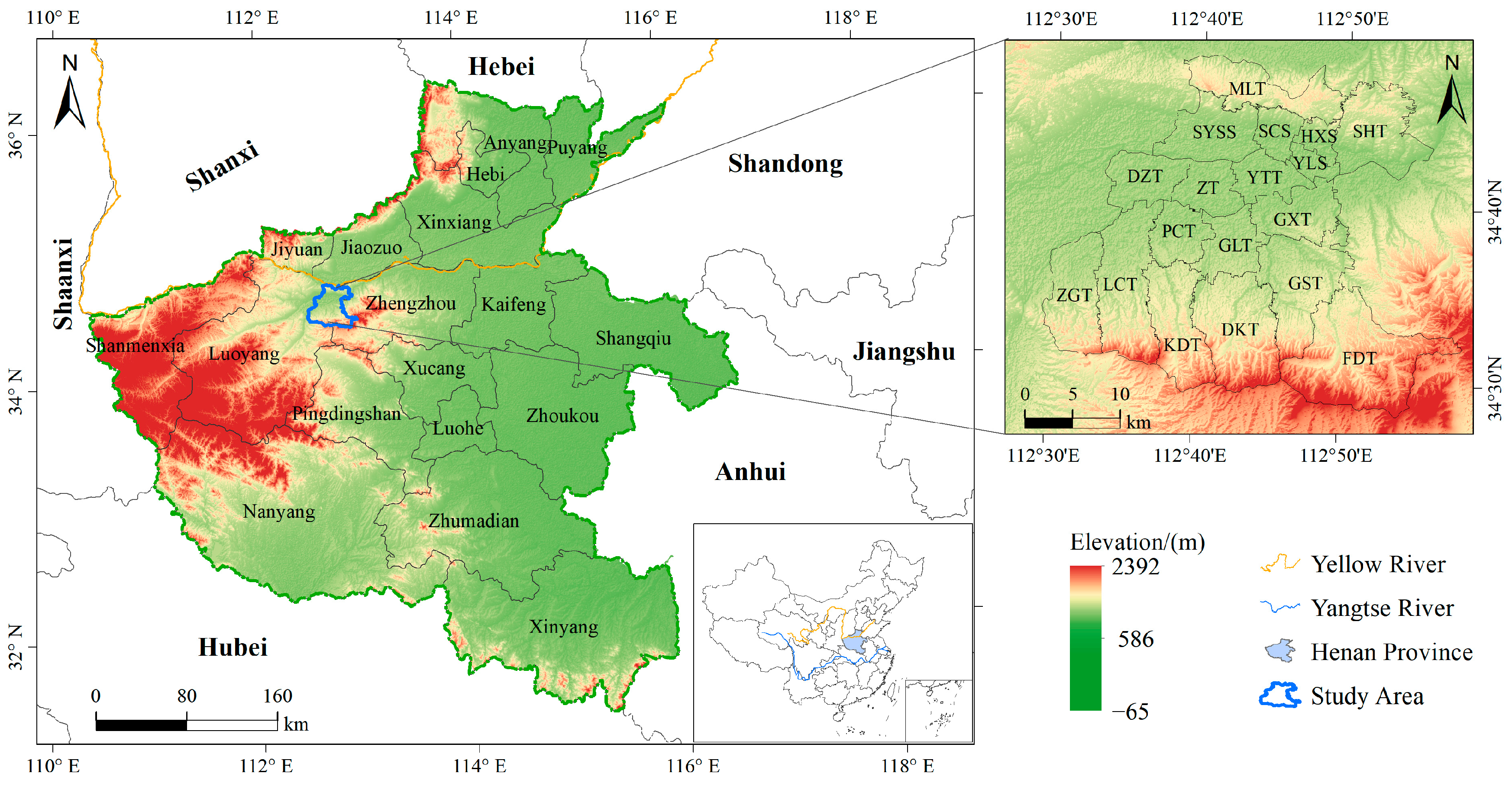
Figure 2.
Geographic location and topography of the research region. Abbreviations for township names: Dianzhuang Town (DZT), Huaixin Street (HXS), Shouyangshan Street (SYSS), Zhai Town (ZT), Yuetang Town (YTT), Guxian Town (GXT), Goushi Town (GST), Fudian Town (FDT), Gaolong Town (GLT), Shanhua Town (SHT), Mangling Town (MLT), Dakou Town (DKT), Shangcheng Street (SCS), Yiluo Street (YLS), Koudian Town (KDT), Pangcun Town (PCT), Licun Town (LCT), and Zhuge Town (ZGT).
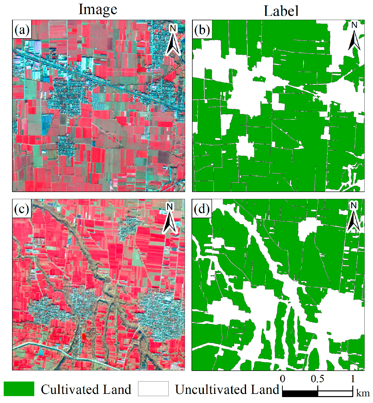
Figure 3.
Sample examples in the study area. (a,c) show the fused standard false-color composite images from GF-2, acquired on 16 December 2020, while (b,d) show the corresponding samples.
Figure 3.
Sample examples in the study area. (a,c) show the fused standard false-color composite images from GF-2, acquired on 16 December 2020, while (b,d) show the corresponding samples.
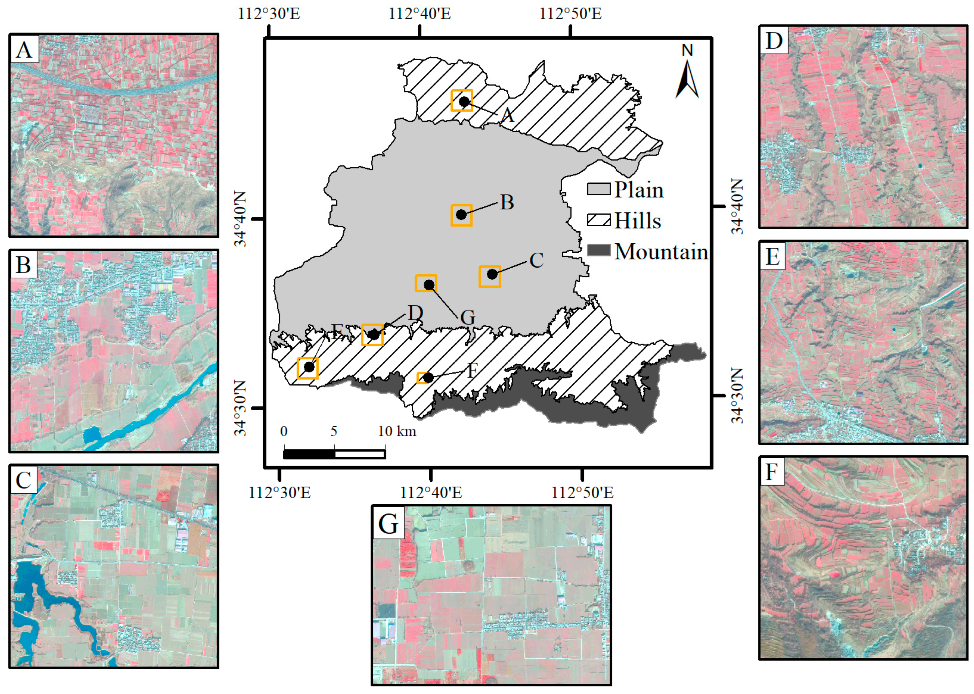
Figure 4.
Location distribution of predicted site. (A–G) are the corresponding GF-2 standard false-color composite images. Site A is in the northern hills, Sites B and C are in the plains, Site D is in the transition zone, and Sites E, F, and G are in the southern hills and plains, respectively. Employing 30 m resolution SRTM DEM data, the research delineated the study area’s landforms into three types based on elevation: plains (0–200 m), hills (200–500 m), and mountains (over 500 m).
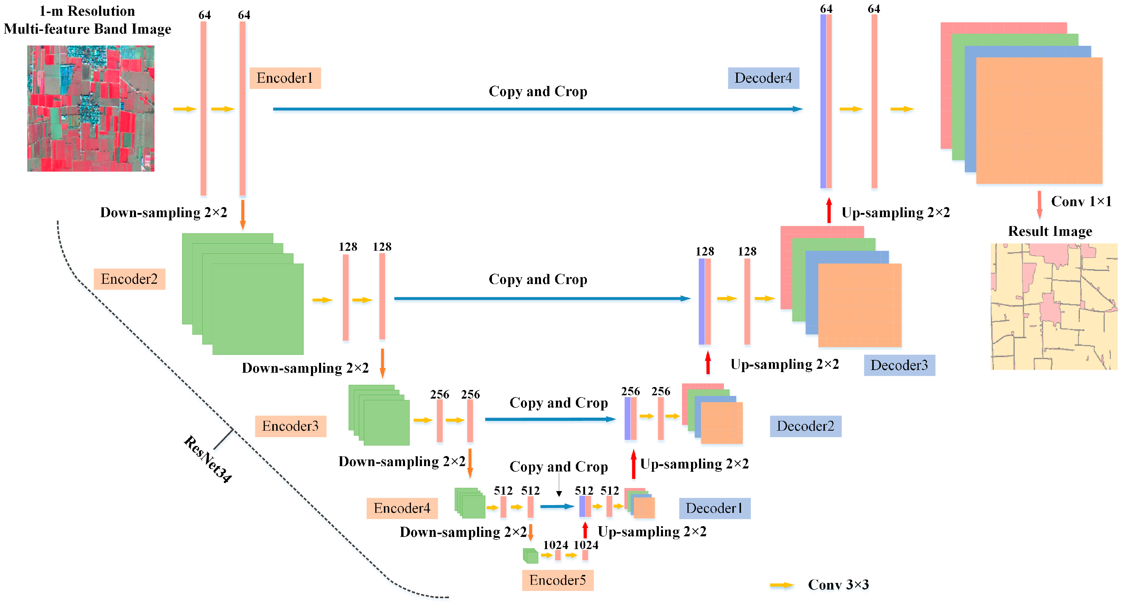
Figure 5.
Improved U-Net architecture employed in the study (built upon Ronneberger et al. [
32]).
Figure 5.
Improved U-Net architecture employed in the study (built upon Ronneberger et al. [
32]).
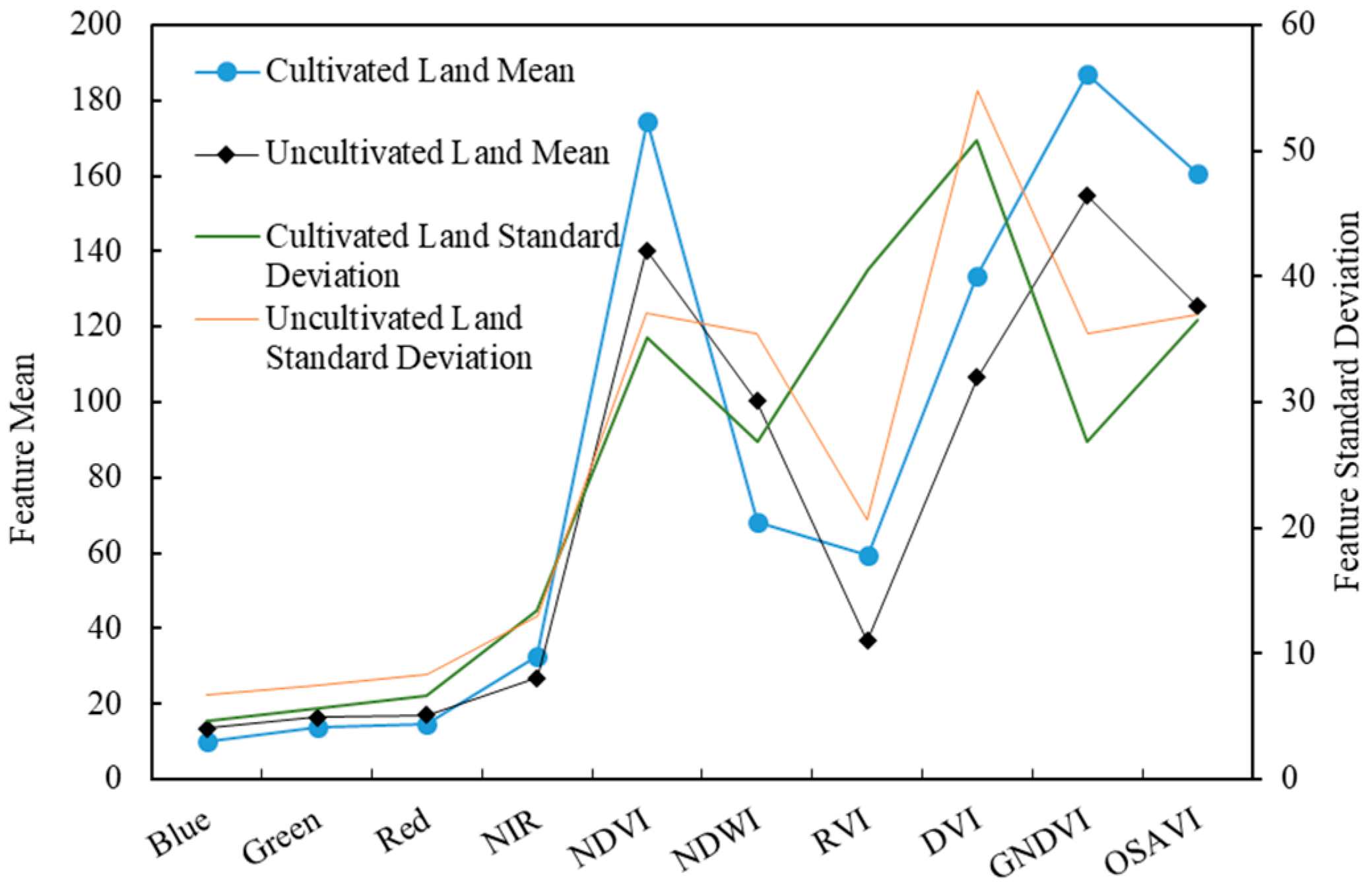
Figure 6.
Mean and standard deviation of each feature.
Figure 6.
Mean and standard deviation of each feature.
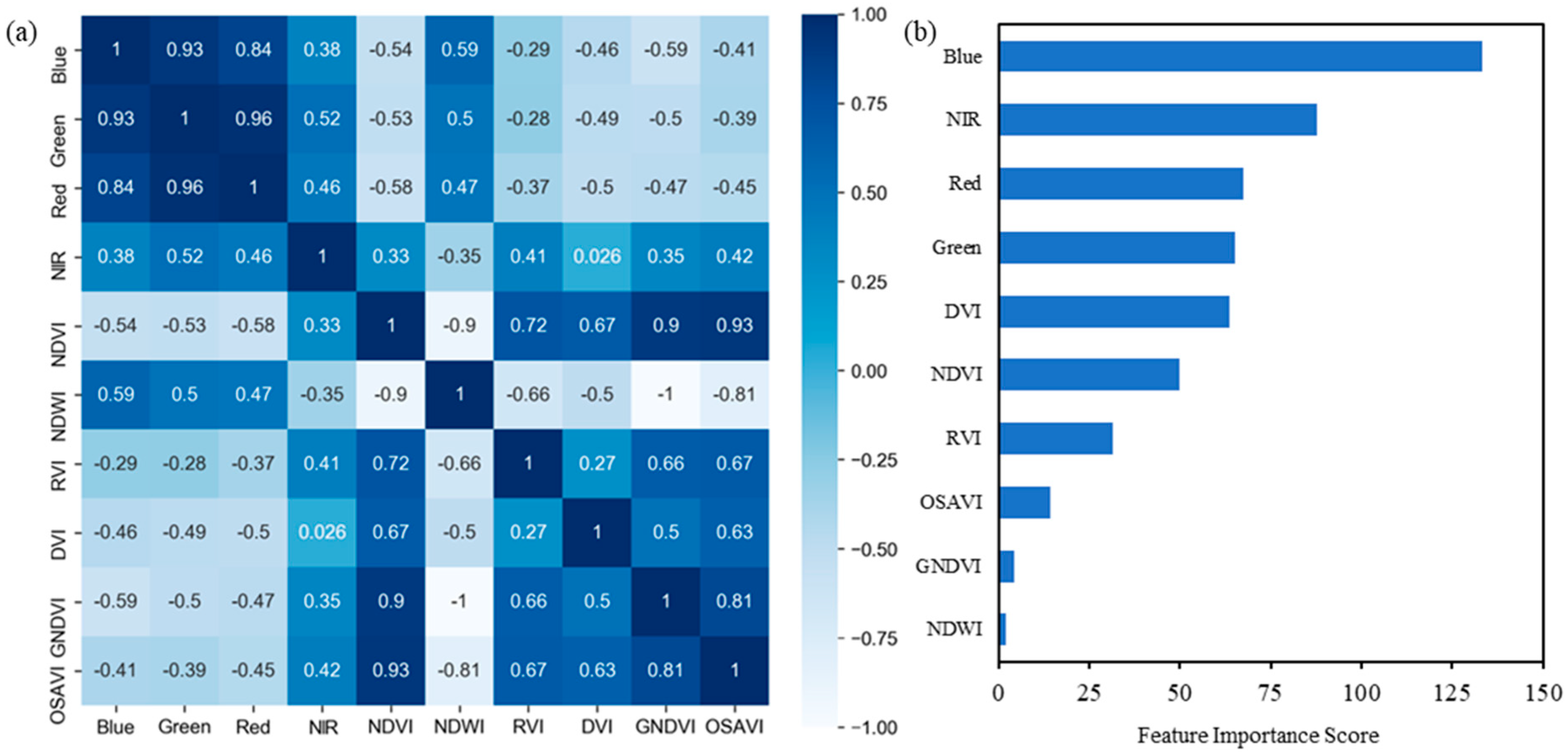
Figure 7.
The PCA and PFI scores results for each feature. (a) shows the pearson correlation analysis results between features. The correlation results among these features are significant at the 0.001 level. (b) shows the permutation feature importance scores for each feature. PFI scores are uniformly multiplied by a constant value of 1000.
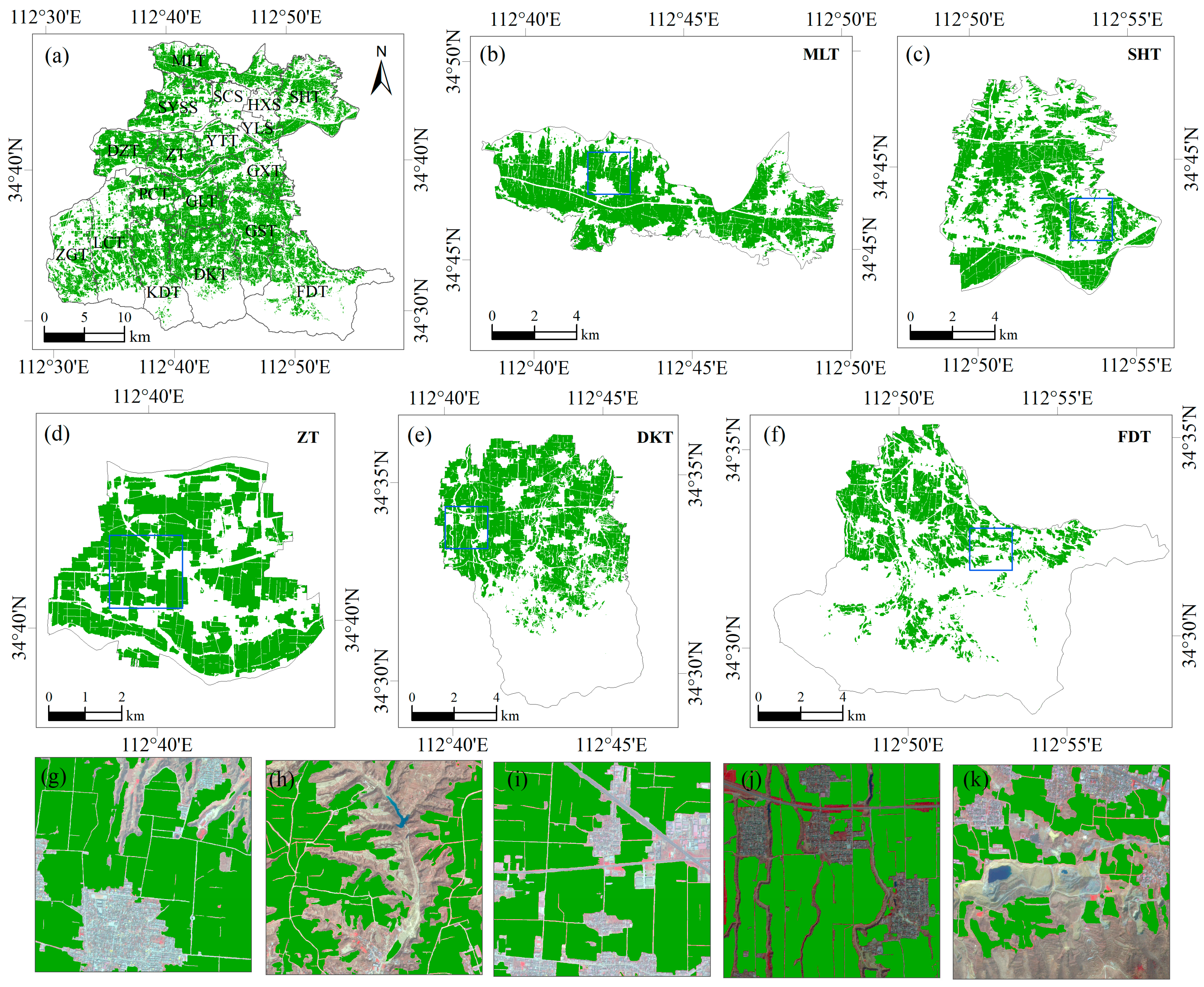
Figure 8.
Cultivated land map spatial details in the study area for 2022. (a) represents the cultivated land extraction results for the entire study area; (b,c) show cultivated land extraction results for the northern hilly region; (d) represents results for the central plain; (e,f) show results for the southern hilly region. (g–k) display zoomed-in views within the blue boxes from (b–f), overlaid with GF-2 standard false-color imagery.
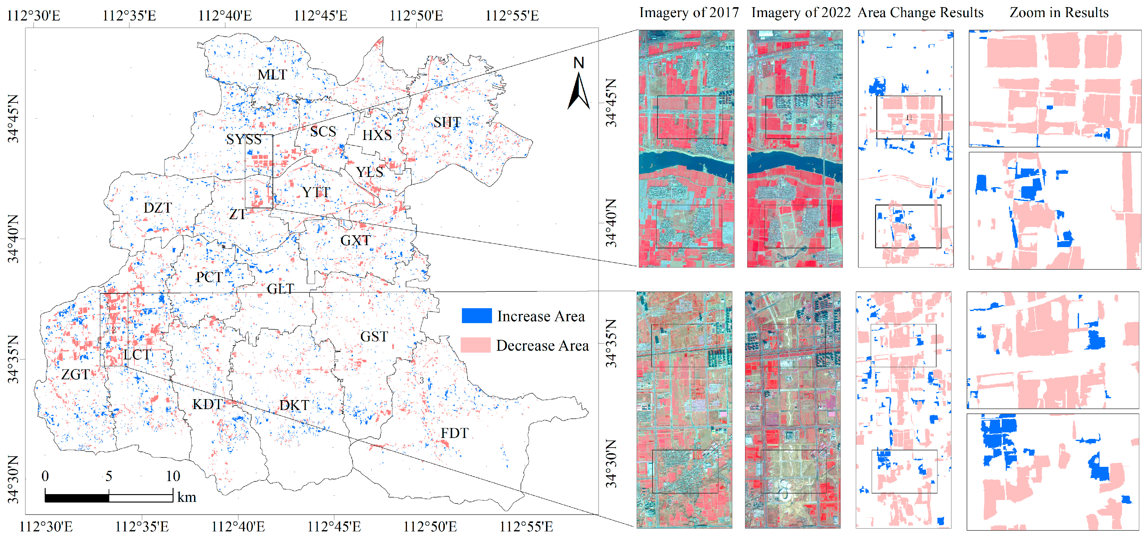
Figure 9.
Cultivated land area changes results from 2017 to 2022.
Figure 9.
Cultivated land area changes results from 2017 to 2022.
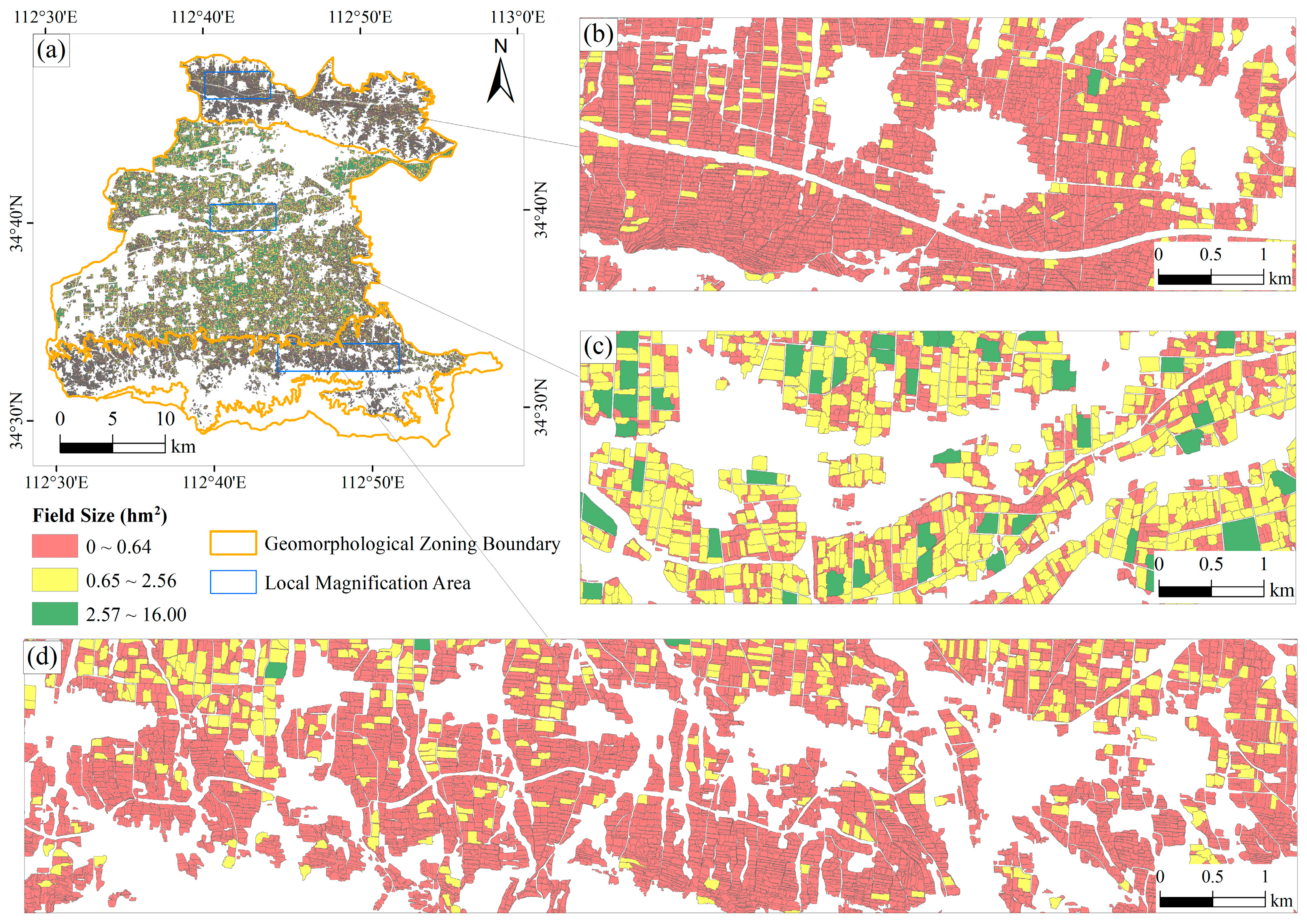
Figure 10.
Map and statistics of field size in the study area for 2020. (a) shows the field size distribution map for the entire study area; (b), (c), and (d) represent the magnified views of the fields in the northern hilly area, central plain area, and southern hilly area of the study region, respectively.
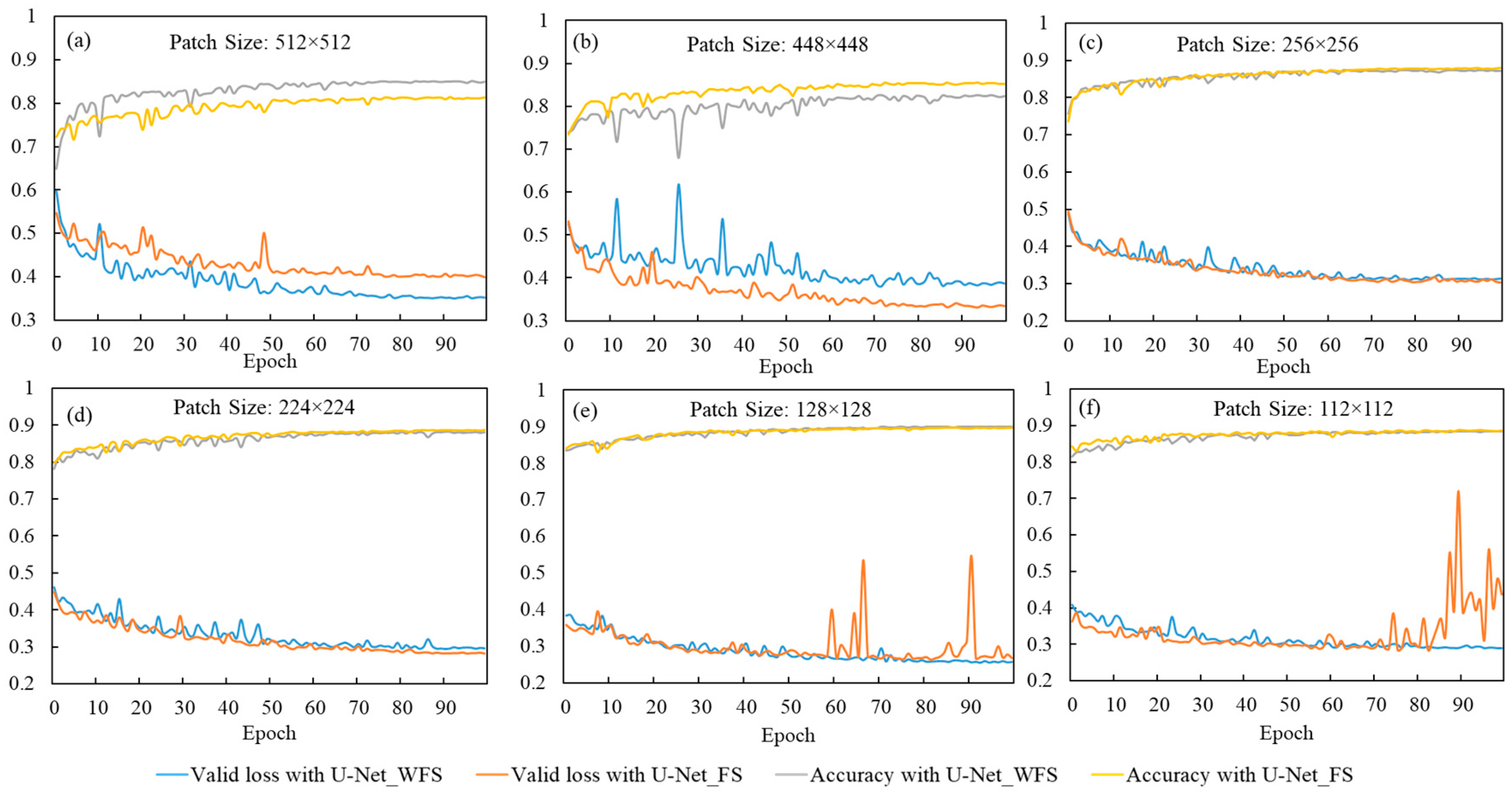
Figure 11.
Training process of U-Net_FS and U-Net_WFS models with different numbers of sample patches. (a–f) represent the changes in model accuracy and validation loss for the U-Net_FS and U-Net_WFS models at patch sizes of 512 × 512 pixels, 448 × 448 pixels, 256 × 256 pixels, 224 × 224 pixels, 128 × 128 pixels, and 112 × 112 pixels, respectively.
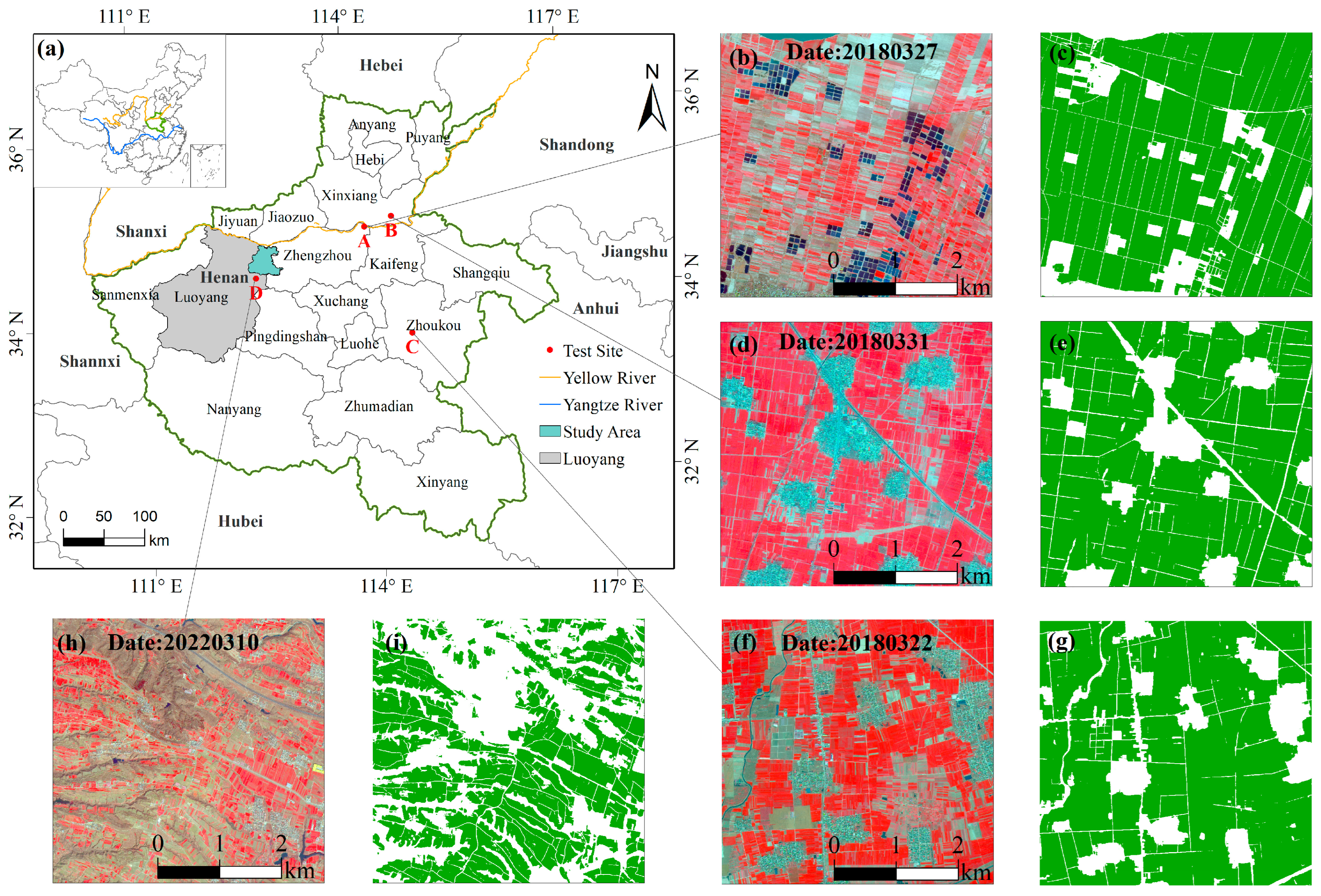
Figure 12.
Cultivated land extraction results in the test areas. Test areas A, B, and C are located in plain regions, while area D represents a hilly region. Green represents cultivated land. (a) shows the schematic map of the test area location; (b,d,f,h) are standard false-color images of GF-2 for test areas A, B, C, and D, respectively; (c,e,g,i) are the corresponding cultivated land extraction results for these images.
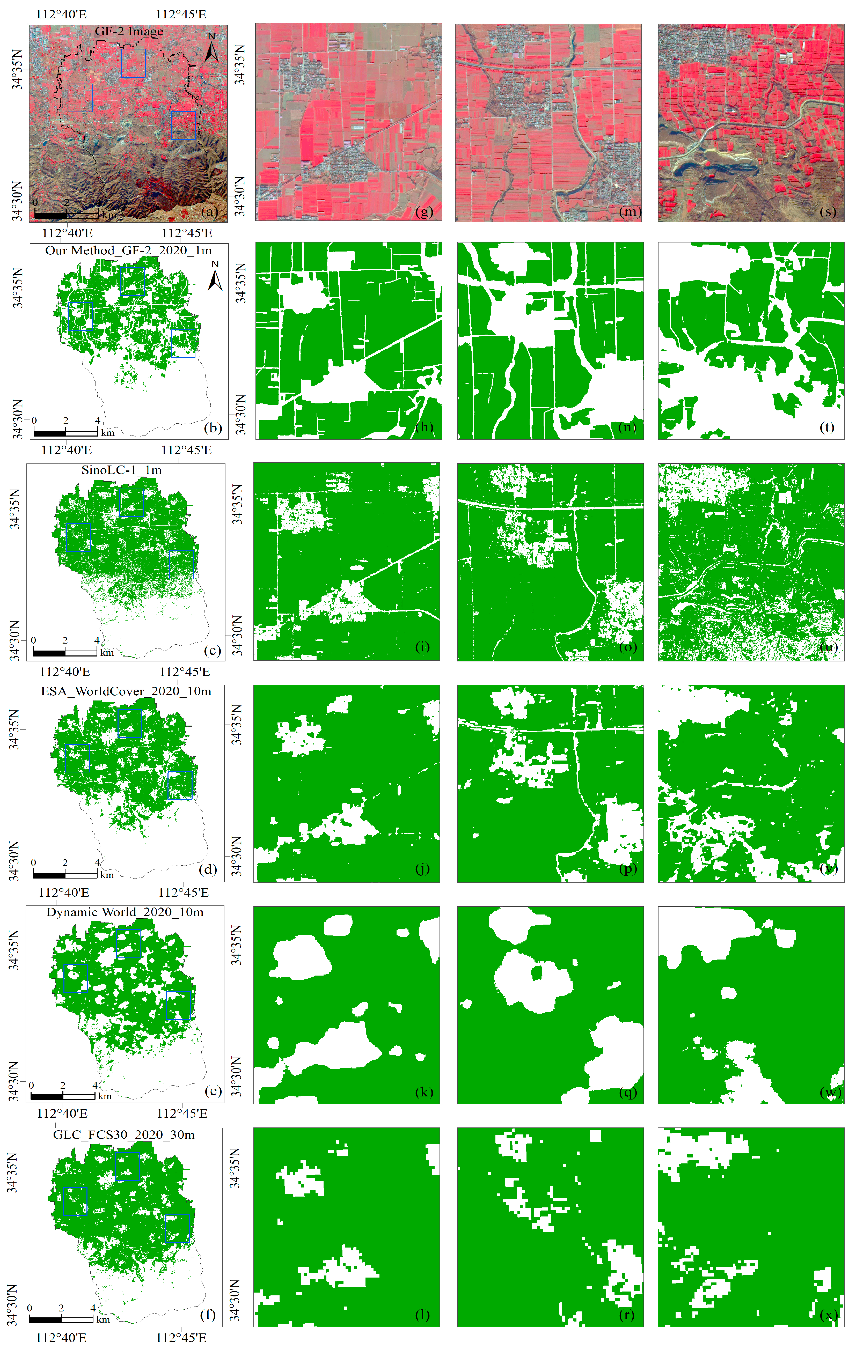
Figure 13.
A visual comparison of the results between the cultivated land extraction method proposed in this study and publicly released cultivated land products. Green represents cultivated land, and (g–x) denotes the zoomed-in views within the blue boxes from (a–f).
Figure 13.
A visual comparison of the results between the cultivated land extraction method proposed in this study and publicly released cultivated land products. Green represents cultivated land, and (g–x) denotes the zoomed-in views within the blue boxes from (a–f).
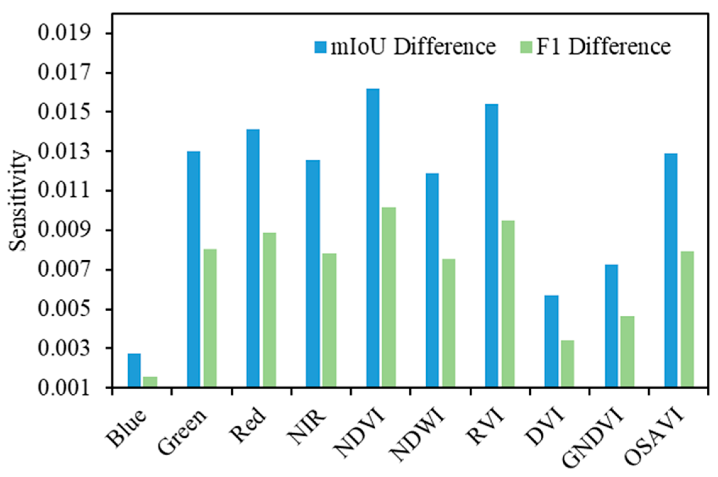
Figure 14.
The classification sensitivity of the U-Net model to each feature.
Figure 14.
The classification sensitivity of the U-Net model to each feature.
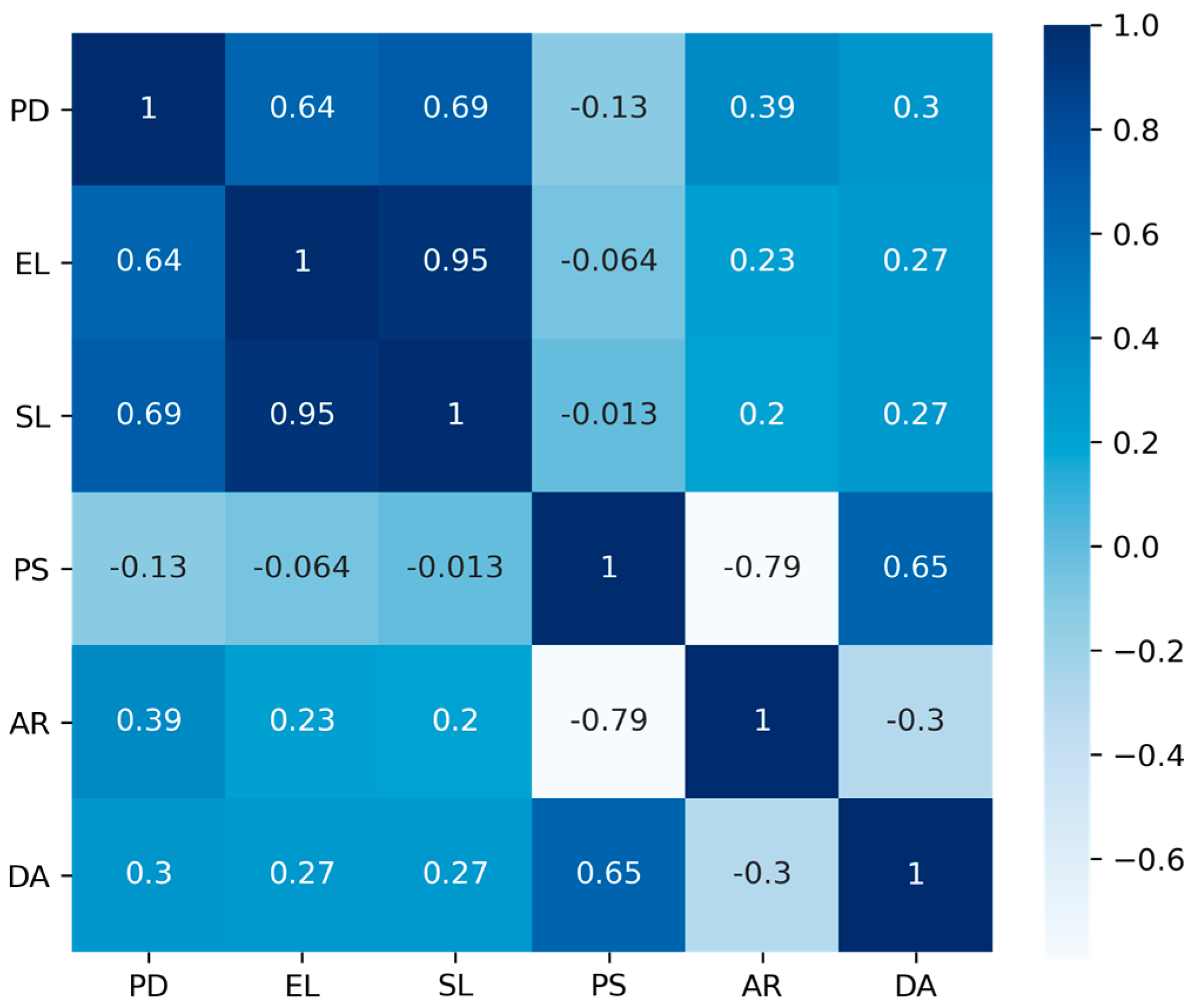
Figure 15.
Correlation between cultivated land fragmentation and potential influencing factors. The result is significant at the 0.001 level.
Figure 15.
Correlation between cultivated land fragmentation and potential influencing factors. The result is significant at the 0.001 level.
Table 1.
GF-2 satellite sensor parameters.
Table 1.
GF-2 satellite sensor parameters.
| Payload | Band Number | Wavelength Range (µm) | Band Name | Spatial Resolution (m) | Revisit Interval (Day) |
|---|
| Panchromatic Multispectral Camera | 1 | 0.45~0.90 | Panchromatic (Pan) | 1 | 5 |
| 2 | 0.45~0.52 | Blue | 4 |
| 3 | 0.52~0.59 | Green |
| 4 | 0.63~0.69 | Red |
| 5 | 0.77~0.89 | Near-Infrared (Nir) |
Table 2.
The area of the quadrat involved in model training from 2017 to 2022 (km2).
Table 2.
The area of the quadrat involved in model training from 2017 to 2022 (km2).
| Year | Month | Cultivated Land | Uncultivated Land | Total Area | The Total Area of Quadrat Each Year |
|---|
| 2017 | 2 | 97.74 | 68.11 | 165.85 | 165.85 |
| 2019 | 7 | 33.77 | 23.47 | 57.24 | 57.24 |
| 2020 | 2 | 8.44 | 5.77 | 14.21 | 449.68 |
| | 8 | 31.31 | 13.69 | 45.00 |
| | 9 | 8.04 | 4.72 | 12.75 |
| | 10 | 53.76 | 27.22 | 80.99 |
| | 11 | 35.07 | 20.32 | 55.39 |
| | 12 | 131.16 | 110.18 | 241.34 |
| 2021 | 11 | 35.07 | 23.84 | 58.91 | 58.91 |
| 2022 | 3 | 93.41 | 66.31 | 159.72 | 159.72 |
Table 3.
Vegetation indices.
Table 3.
Vegetation indices.
| ID | Vegetation Index | Expression |
|---|
| 1 | NDVI | (NIR − Red)/(NIR + Red) |
| 2 | NDWI | (Green − NIR)/(Green + NIR) |
| 3 | RVI | NIR/Red |
| 4 | DVI | NIR − Red |
| 5 | GNDVI | (NIR − Green)/(NIR + Green) |
| 6 | OSAVI | (NIR − Red)/(NIR + Red + 0.16) |
Table 4.
Design scheme of the cultivated land information extraction model.
Table 4.
Design scheme of the cultivated land information extraction model.
| Scheme | Band Composition | Description |
|---|
| U-Net_WFS | Blue, Green, Red, NIR | Spectral Features |
| U-Net_FS | Blue, Green, Red, NIR, NDVI, RVI, DVI, OSAVI | Spectral Features + Vegetation Features |
Table 5.
Assessment results of cultivated land extraction under various landforms.
Table 5.
Assessment results of cultivated land extraction under various landforms.
| Site | Physiognomy | Evaluation Metrics | Scheme |
|---|
| U-Net_WFS | U-Net_FS |
|---|
| Cultivated Land | Uncultivated Land | Cultivated Land | Uncultivated Land |
|---|
| A | Northern Hilly Area | IoU | 0.8632 | 0.7363 | 0.8712 | 0.7582 |
| PA | 0.9380 | 0.8272 | 0.9538 | 0.8234 |
| UA | 0.9153 | 0.8702 | 0.9095 | 0.9055 |
| F1 | 0.8877 | 0.8980 |
| OA | 0.9010 | 0.9082 |
| Kappa | 0.7748 | 0.7939 |
| B | Plain | IoU | 0.9095 | 0.8867 | 0.9151 | 0.8912 |
| PA | 0.9665 | 0.9231 | 0.9596 | 0.9375 |
| UA | 0.9392 | 0.9573 | 0.9518 | 0.9474 |
| F1 | 0.9465 | 0.9491 |
| OA | 0.9470 | 0.9499 |
| Kappa | 0.8926 | 0.8981 |
| C | Plain | IoU | 0.9416 | 0.8600 | 0.9439 | 0.8653 |
| PA | 0.9862 | 0.8881 | 0.9875 | 0.8909 |
| UA | 0.9542 | 0.9646 | 0.9553 | 0.9678 |
| F1 | 0.9481 | 0.9503 |
| OA | 0.9570 | 0.9588 |
| Kappa | 0.8947 | 0.8990 |
| D | Transition Zone between Plains and Hilly Areas | IoU | 0.8876 | 0.8072 | 0.9024 | 0.8271 |
| PA | 0.9722 | 0.8440 | 0.9701 | 0.8700 |
| UA | 0.9107 | 0.9488 | 0.9282 | 0.9437 |
| F1 | 0.9188 | 0.9279 |
| OA | 0.9236 | 0.9335 |
| Kappa | 0.8341 | 0.8542 |
| E | Southern Hilly Area | IoU | 0.8021 | 0.7589 | 0.8401 | 0.8092 |
| PA | 0.8606 | 0.9015 | 0.8934 | 0.9192 |
| UA | 0.9218 | 0.8274 | 0.9338 | 0.8711 |
| F1 | 0.8779 | 0.9044 |
| OA | 0.8781 | 0.9047 |
| Kappa | 0.7535 | 0.8078 |
| F | Southern Hilly Area | IoU | 0.5885 | 0.7447 | 0.6336 | 0.8176 |
| PA | 0.6681 | 0.9097 | 0.8083 | 0.8837 |
| UA | 0.8317 | 0.8042 | 0.7456 | 0.9162 |
| F1 | 0.8032 | 0.8384 |
| OA | 0.8130 | 0.8613 |
| Kappa | 0.5974 | 0.6756 |
Table 6.
Evaluation of cultivated land extraction results under different temporal phases.
Table 6.
Evaluation of cultivated land extraction results under different temporal phases.
| Image Date | Evaluation Metrics | Scheme |
|---|
| U-Net_WFS | U-Net_FS |
|---|
| Cultivated Land | Uncultivated Land | Cultivated Land | Uncultivated Land |
|---|
| 20170211 | IoU | 0.9358 | 0.7249 | 0.9336 | 0.7159 |
| PA | 0.9768 | 0.8012 | 0.9753 | 0.7963 |
| UA | 0.9571 | 0.8839 | 0.9561 | 0.8764 |
| F1 | 0.9045 | 0.9008 |
| OA | 0.9451 | 0.9431 |
| Kappa | 0.8074 | 0.8002 |
| 20171209 | IoU | 0.9041 | 0.6468 | 0.9022 | 0.6345 |
| PA | 0.9482 | 0.7907 | 0.9434 | 0.7955 |
| UA | 0.9511 | 0.7804 | 0.9539 | 0.7582 |
| F1 | 0.8676 | 0.8627 |
| OA | 0.9184 | 0.9164 |
| Kappa | 0.7351 | 0.7250 |
| 20190713 | IoU | 0.9077 | 0.6652 | 0.9099 | 0.6732 |
| PA | 0.9676 | 0.7478 | 0.9695 | 0.7513 |
| UA | 0.9362 | 0.8577 | 0.9367 | 0.8663 |
| F1 | 0.8769 | 0.8804 |
| OA | 0.9220 | 0.9240 |
| Kappa | 0.7509 | 0.7578 |
| 20201216 | IoU | 0.8874 | 0.6564 | 0.8915 | 0.6610 |
| PA | 0.9629 | 0.7330 | 0.9601 | 0.7476 |
| UA | 0.9189 | 0.8628 | 0.9258 | 0.8509 |
| F1 | 0.8688 | 0.8708 |
| OA | 0.9074 | 0.9105 |
| Kappa | 0.7335 | 0.7389 |
| 20211112 | IoU | 0.9316 | 0.7709 | 0.9295 | 0.7683 |
| PA | 0.9724 | 0.8458 | 0.9752 | 0.8330 |
| UA | 0.9569 | 0.8970 | 0.9520 | 0.9082 |
| F1 | 0.9179 | 0.9169 |
| OA | 0.9444 | 0.9429 |
| Kappa | 0.8353 | 0.8325 |
| 20220310 | IoU | 0.9251 | 0.7435 | 0.9290 | 0.7565 |
| PA | 0.9704 | 0.8232 | 0.9734 | 0.8285 |
| UA | 0.9520 | 0.8849 | 0.9531 | 0.8969 |
| F1 | 0.9075 | 0.9128 |
| OA | 0.9385 | 0.9418 |
| Kappa | 0.8141 | 0.8246 |
Table 7.
Evaluation results of different methods for cultivated land extraction from high-resolution imagery.
Table 7.
Evaluation results of different methods for cultivated land extraction from high-resolution imagery.
| Model | mIoU | Recall | Precision | F1 |
|---|
| PSPNet | 76.61% | 92.84% | 81.60% | 86.86% |
| DeepLabV3 | 79.43% | 91.67% | 85.83% | 88.65% |
| U-Net | 80.19% | 93.94% | 84.73% | 89.10% |
| Our method | 80.88% | 94.65% | 84.96% | 89.55% |
Table 8.
Cultivated land area changes at the township scale in the study area from 2017 to 2022 (km2).
Table 8.
Cultivated land area changes at the township scale in the study area from 2017 to 2022 (km2).
| Township Name | Total Land Area of the Township | Cultivated Land Area in 2017 | Increase Area | Decrease Area | Ultimate Change Area |
|---|
| DZT | 38.47 | 22.64 | 0.78 | −0.87 | −0.09 |
| HXS | 14.46 | 2.30 | 0.33 | −0.80 | −0.47 |
| SYSS | 53.58 | 25.77 | 2.03 | −2.83 | −0.81 |
| ZT | 31.81 | 19.51 | 0.76 | −1.51 | −0.75 |
| YTT | 29.31 | 12.63 | 0.70 | −1.58 | −0.88 |
| GXT | 43.85 | 22.82 | 1.16 | −2.26 | −1.10 |
| GST | 80.30 | 49.97 | 1.16 | −2.48 | −1.32 |
| FDT | 127.09 | 27.48 | 1.12 | −2.42 | −1.30 |
| GLT | 37.59 | 23.92 | 0.76 | −0.76 | 0.00 |
| SHT | 68.20 | 35.29 | 1.71 | −3.03 | −1.32 |
| MLT | 58.43 | 33.38 | 1.61 | −1.20 | 0.41 |
| DKT | 88.42 | 37.86 | 1.41 | −1.92 | −0.51 |
| SCS | 20.79 | 3.33 | 0.73 | −0.81 | −0.08 |
| YLS | 11.85 | 4.34 | 0.15 | −0.88 | −0.73 |
| KDT | 63.97 | 24.08 | 1.19 | −2.06 | −0.87 |
| PCT | 32.88 | 17.88 | 1.35 | −0.86 | 0.49 |
| LCT | 83.89 | 33.35 | 3.14 | −7.29 | −4.15 |
| ZGT | 60.73 | 22.64 | 2.46 | −4.23 | −1.77 |
| Total area | 945.62 | 419.19 | 22.55 | −37.81 | −15.26 |
Table 9.
Field size statistics of the study area.
Table 9.
Field size statistics of the study area.
| Field Size | Field Count | Proportion of Total Fields |
|---|
| Very small | 80,935 | 83.84% |
| Small | 14,535 | 15.06% |
| Medium | 1061 | 1.10% |
Table 10.
The model accuracy for U-Net_WFS and U-Net_FS under different patch sizes.
Table 10.
The model accuracy for U-Net_WFS and U-Net_FS under different patch sizes.
| Patch Size (Pixels) | mIoU | F1 | Mean Epoch Time (s) |
|---|
| U-Net_WFS | U-Net_FS | U-Net_WFS | U-Net_FS | U-Net_WFS | U-Net_FS |
|---|
| 512 × 512 | 0.7369 | 0.6768 | 0.8434 | 0.7990 | 201 | 232 |
| 448 × 448 | 0.6963 | 0.7391 | 0.8106 | 0.8463 | 187 | 219 |
| 256 × 256 | 0.7673 | 0.7768 | 0.8767 | 0.8841 | 212 | 243 |
| 224 × 224 | 0.7821 | 0.7914 | 0.8846 | 0.8892 | 218 | 261 |
| 128 × 128 | 0.8099 | 0.8047 | 0.9051 | 0.9020 | 324 | 360 |
| 112 × 112 | 0.7804 | 0.7882 | 0.8880 | 0.8929 | 400 | 411 |
Table 11.
The model accuracy under different training sample sizes.
Table 11.
The model accuracy under different training sample sizes.
| Patch Size Number | 1950 | 3901 | 5851 | 7801 | 9752 | 11,702 | 13,652 | 15,602 | 17,553 |
| Percentage of Patch Number | 10% | 20% | 30% | 40% | 50% | 60% | 70% | 80% | 90% |
| mIoU | 0.6511 | 0.6981 | 0.7735 | 0.7597 | 0.7699 | 0.7612 | 0.7670 | 0.7733 | 0.7783 |
| F1 | 0.8309 | 0.8457 | 0.8843 | 0.8742 | 0.8791 | 0.8794 | 0.8836 | 0.8837 | 0.8867 |
| Mean Epoch Time (s) | 290 | 360 | 435 | 439 | 540 | 620 | 630 | 732 | 787 |
Table 12.
The model accuracy of U-Net_WFS and U-Net_FS under multi-temporal samples.
Table 12.
The model accuracy of U-Net_WFS and U-Net_FS under multi-temporal samples.
| Model | mIoU | Precision | Recall | F1 | Total Duration of Model Training (h) |
|---|
| U-Net_FS | 80.88% | 84.96% | 94.65% | 89.55% | 26.5 |
| U-Net_WFS | 80.19% | 84.73% | 93.94% | 89.10% | 20.3 |
Table 13.
Information on publicly released cultivated land products used in this study.
Table 13.
Information on publicly released cultivated land products used in this study.
| Name | Year | Spatial Resolution (m) | Data Source | OA |
|---|
| ESA_WorldCover | 2020 | 10 | Sentinel-1/2 | 74.4% |
| Dynamic World | 2020 | 10 | Sentinel-2 | / |
| GLC_FCS | 2020 | 30 | Landsat TM, ETM+ and OLI | 77.34% |
| SinoLC-1 | / | 1 | Google | 73.61% |


 ,
, 
