Abstract
Evapotranspiration (ET) rates will be affected by climate change and increasing frequency of extreme heat events. To understand how forests may respond to probable future climate conditions, it may be helpful to look at the past relationship between climate and ET. This can be accomplished using satellite imagery since the 1980s, but prior to that, a different approach is required. Using a global ET dataset (1982 to 2010) with 1 km resolution, climate station information from 1850 to 2010, and 54 tree-ring plots from the International Tree-Ring Data Bank (ITRDB) database, ET reconstructions were developed for each vegetated pixel with point-by-point regressions in British Columbia. ET was estimated for the province of British Columbia in Canada from 1850 to 1981, using random forest, support vector machine, and convolutional neural network regressions. ET satellite images from 1982 to 2010 formed our dataset to train models for each vegetated pixel. The random forest regression outperformed the other approaches with lower errors and better robustness (adjusted R2 value = 0.69; root mean square error = 10.72 mm/month). Modeled findings indicate that ET rates are generally increasing in British Columbia (ET = 0.0064 × Year + 52.339), but there were regional effects on local ET, as only the Humid Temperate ecodomain had strong correlations of ET with mean summer temperature (r = 0.257, p < 0.01) and mean summer precipitation (r = −0.208, p < 0.05). These historical estimates provide an opportunity to observe spatiotemporal variation in ET across British Columbia and elsewhere.
1. Introduction
Evapotranspiration (ET) is a key component of the global water cycle that also plays a significant role in the heat balance of the ecosphere [1,2]. ET includes evaporation and transpiration sub-processes, where evaporation refers to the movement of liquid water to its gaseous form in the atmosphere, while transpiration refers to the loss of water from plants via stomata to the atmosphere [3,4]. Transpiration regulates plant temperature and facilitates the flow of water and minerals from the root to the canopy [5]. ET is an indicator of vegetation growth, and a number of studies have measured or modeled ET values at a variety of scales [6,7]. Zhang et al. [8] applied a Three-Temperature Model to measure a vegetated roof with two grass species (Zoysia tenuifoli and Callisia repens) with high precision in Shengzhen, China. Mao and Wang [9] applied a modified Penman–Monteith (MPM) model for the whole of China from 1982 to 2010 using 2479 weather stations and identified that the ET pattern in China was determined by precipitation. Elnashar et al. [10] went even further by developing a monthly ET global dataset from 1982 to 2019 with a spatial resolution of 1 km, using multiple satellite data sources.
Previous work in this area has been focused on periods since satellite and broader weather station information has been available [10,11,12]. To address ET rates before 1980, some studies have used tree rings as a proxy for ET. For example, Zhou et al. [13] reconstructed the Standardized Precipitation Evapotranspiration Index (SPEI) with Chinese cedar cores (Toona sinensis) in Fujian Province, China, and determined that floods have a close relationship with the El Niño–Southern Oscillation (ENSO). Similarly, Cabral-Alemán et al. [14] conducted a SPEI reconstruction with a Durango pine (Pinus durangensiplot) in Durango State, Mexico, and found that early wood residual had a positive relationship with the cumulative SPEI for February–May. These studies, like much previous research, have treated their whole study areas as a single point, ignoring potential heterogeneous response across the landscape. Few studies have attempted to generate paleo-ET data for large spatial extents, even though it is desirable to understand historical ET patterns. Li et al. [15,16] have begun to bridge this gap by integrating tree-ring data and remote-sensing images since the 1980s. They mapped the paleo-vegetation spatial distribution using point-by-point regression to reconstruct paleo-vegetation index time-series maps in what was the first study to present the spatiotemporal variation of paleo-vegetation and provide insight into historical vegetation dynamics across a large landscape. This past work has shown the need for machine-learning or deep-learning modeling because there can be poor correlation between the Normalized Difference Vegetation Index (NDVI) and tree-ring plot data at broad landscape scales [17].
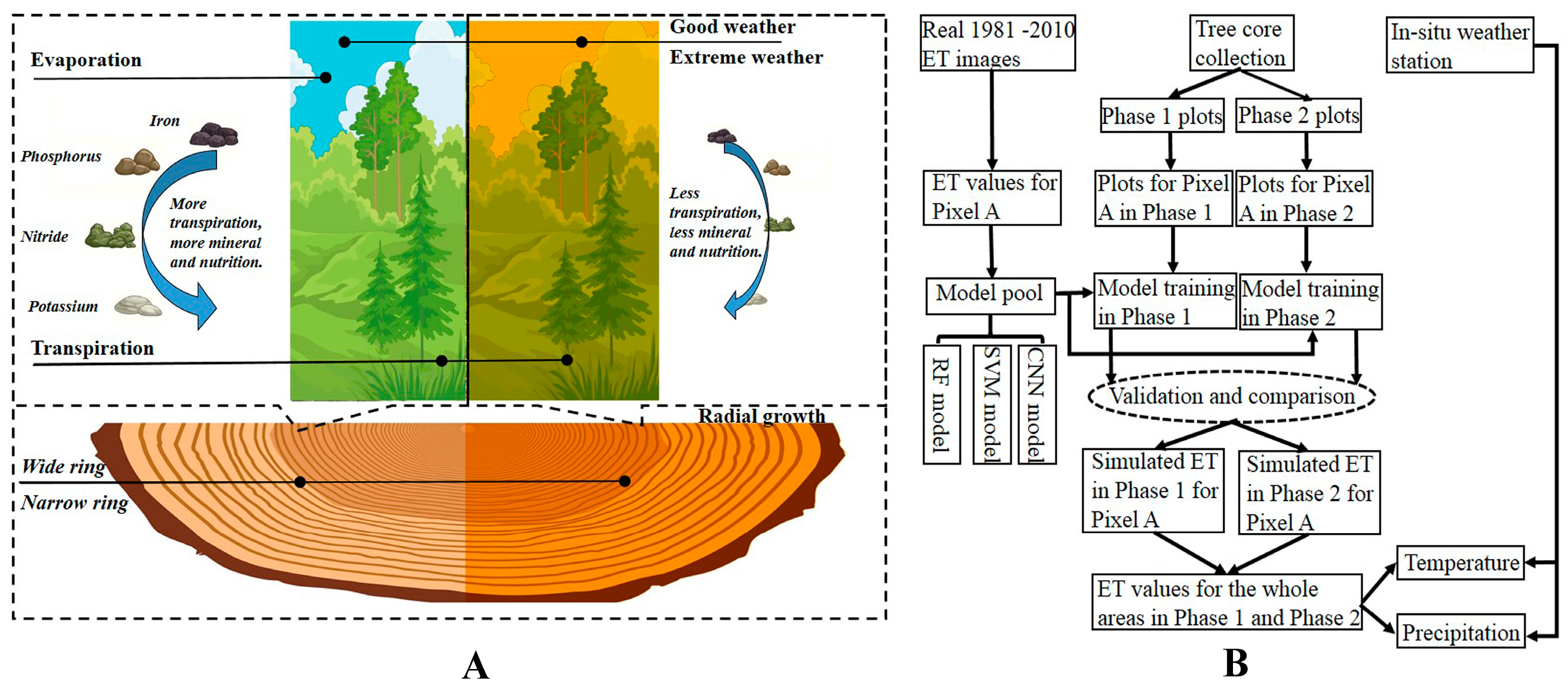
Reconstruction of ET levels using tree-ring data in this earlier work demonstrated that there is a relationship between tree radial growth and ET [13,14] and that the model could simulate the paleo-ET with tree-ring index as a proxy. Radial growth requires nutrients, including minerals transported by transpiration, so the ring width can serve as an indicator to evaluate ET in vegetated areas (Figure 1A). Using publicly available tree-ring data here to estimate past ET levels in British Columbia, our study hypothesizes that ET has increased from 1850 to 2010 due to increasing air temperature and climate change. Rising temperatures in the growing season and the extension of the frost-free period might be expected to increase ET. Warmer temperatures can increase the rate of evaporation from soil surfaces and transpiration from plants and lead to an upward trend in ET.
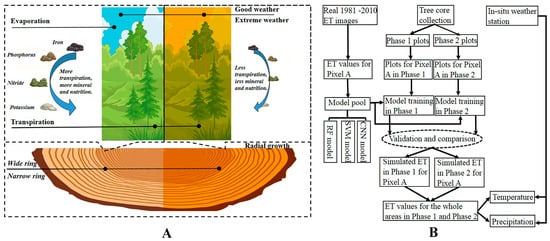
Figure 1.
Theoretical relationship between weather, ET, and tree-ring width (A), and the workflow. Note: In (A), nutrients and minerals necessary for the radial growth are transported via transpiration, which indicates that the width of the tree ring can be a good proxy for ET. In (B), pixel A refers to any vegetated pixel within the province of British Columbia (Phase 1 refers to the 50 tree-ring data plots available covering 1850–1981, and Phase 2 refers to the 54 plots from 1890 to 2010).
2. Methods
This study used tree-ring data, ET satellite images, and climate records to elucidate interactions among ET, tree-ring index, and climate. Satellite-based ET estimates were available for each vegetated pixel from 1982 to 2010. Three machine-learning approaches were used to develop the relationship between ET data for that pixel (identified as Pixel A in 1B) and nearby tree-ring information, after which the most robust model was selected to estimate ET from tree-ring data from 1850 to 1981 (Figure 1B).
2.1. Study Areas and Data Collection
Our study area is British Columbia, Canada, which is 944,735 km2 in size (Figure 2A). Its forests are ecologically diverse and cover approximately 544,000 km2 of the province, with about 41% of the forest areas identified as old growth (>140 years) in 2015 [18]. The province can be divided into the Polar, Humid Temperate, and Dry ecodomains, which are areas of broadly similar climate [19] (Figure 2B). There are many native tree species in the province, including Engelmann spruce (Picea engelmannii), mountain hemlock (Tsuga mertensiana), ponderosa pine (Pinus ponderosa), Douglas fir (Pseudotsuga menziesii), and others.
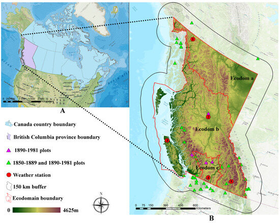
Figure 2.
Site map with the locations of tree-ring plots and weather stations. Note: In (A), the pink polygon (British Columbia, Canada) is our study area. In (B), weather stations 1, 2, 3, 4, and 5 are Atlin, Fort St. James, Quatsino, Hedley NP Mine, and Golden A, respectively. In (B), Ecodomain a, Ecodomain b, and Ecodomain c are the Polar ecodomain, Humid Temperate ecodomain, and Dry ecodomain, respectively.
To estimate historical ET, our study utilized three publicly available data sources, namely tree-ring data, remote-sensing images, and in situ weather station records. There were 54 tree-ring plots within the province and the 150 km buffer available from the International Tree-Ring Database (ITRDB, https://www.ncei.noaa.gov/products/paleoclimatology/tree-ring, accessed on 5 January 2025), which is one of the largest publicly available global datasets hosting thousands of tree-ring records (Figure 2B) (plot information in Appendix A Table A1). The dataset provides the tree-ring index for each plot, as well as tree species, coordinate position, topographic position, and other essential background information. The AutoRegressive STANdardization (ARSTAN, Tree-Ring Laboratory, Lamont Doherty Earth Observatory of Columbia University, New York, NY, USA) program [20] was used to detrend the tree-ring width with self-dependent splines [21] to calculate tree-ring indices (TRIs). The expressed population signal (EPS) threshold was 0.85. Tree-ring plots were subdivided into two periods, namely the 1850–2010 period (where 50 plots were available) and the 1890–2010 period (when another 4 plots were available).
The remote-sensing ET data were available from the global monthly ET database from 1982 to 2010 and had a spatial resolution of 1 km; the dataset had outcompeted multiple global and local ET datasets with low relative mean error (13.94 mm) and relative root mean square error (38.61 mm) [10]. The summer (June, July, and August) ET ranging from 1982 to 2010 was extracted. Our study averaged three months of data and acquired the annual summer ET series maps.
Previous studies [15] indicated that these reconstructions would have great performances for forest and grassland, so water, urban areas, and barren areas were masked out using the Canada Landcover Database 2010 [22] and British Columbia administrative boundary layer (https://www2.gov.bc.ca/gov/content/data/geographic-data-services/land-use/administrative-boundaries, accessed on 20 December 2024). Our study only ran the regression models for each vegetated pixel (forest and grass). The processed annual time-series maps only included the ET in the forest and grassland from 1982 to 2010. Data processing was completed using Google Earth Engine.
Weather station data were gathered from five locations that covered most if not all this period of record. Stations included Atlin, Fort St. James, Golden A, Quatsino, and Hedley Np Mine (Figure 2B). Ideally, each station would have data from 1850 to 2010, but for some stations, reliable monthly data were only available from 1904 onward. Data were summarized to generate mean monthly summer temperature (June, July, and August), the mean maximum summer temperature, and mean monthly summer precipitation. ARSTAN identified that some plots had one-year lag. Other research identified the importance of snow depth on vegetation growth [23], so mean monthly and mean minimum temperature in the previous winter (December, January, and February), as well as mean monthly precipitation and snow in the previous winter, were included in the analysis.
2.2. Tree-Ring ET Model
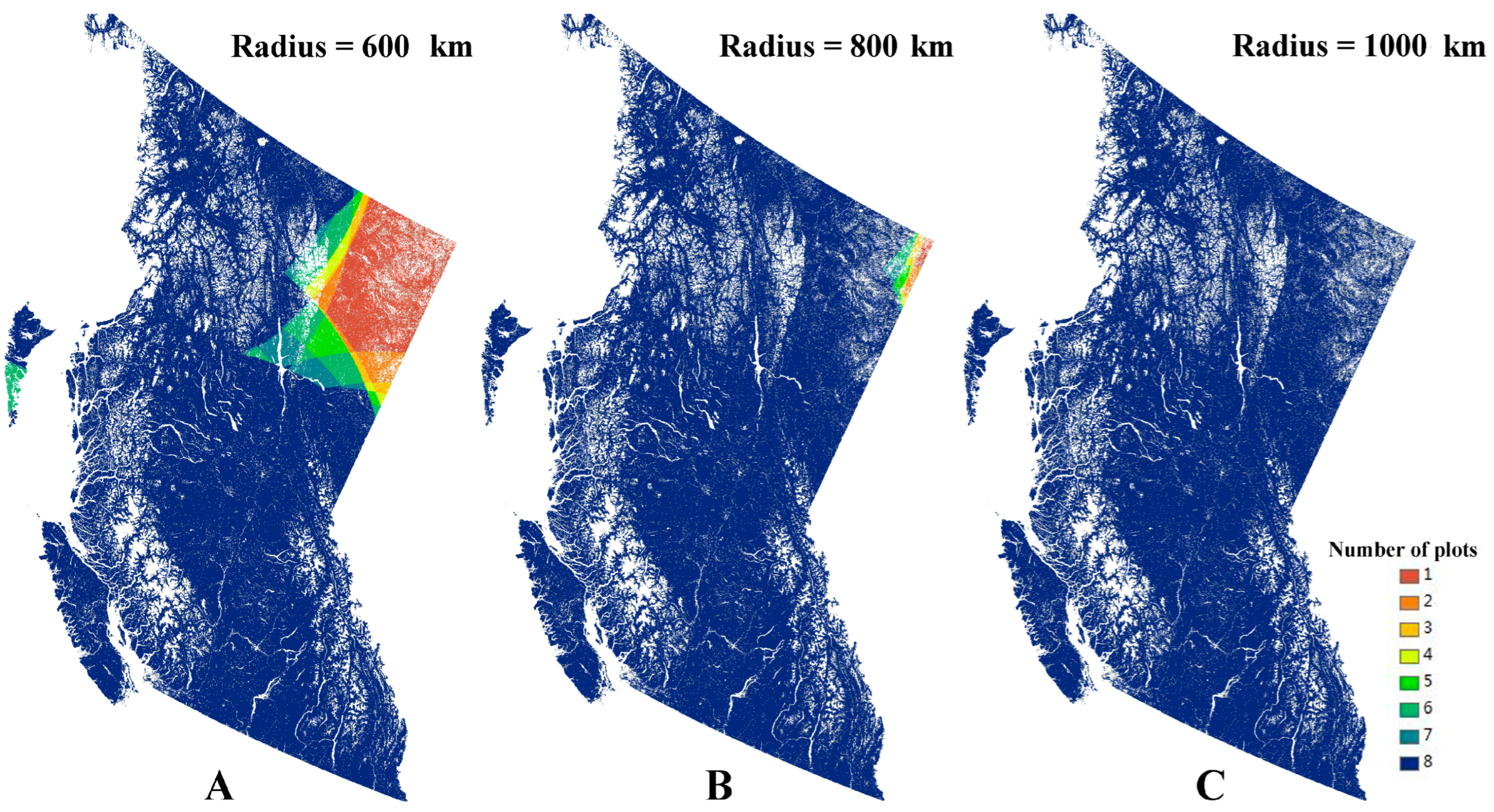
There were 50 tree-ring plots available for 1850–1982 and 54 plots for the 1890–1982 time period, so two reconstructions were conducted to ensure all available data were used and that chronological integrity was maintained. Each pixel was 1 km2 and considered to be the center of a circle with all tree-ring plot data within a 600 km, 800 km, and 1000 km distance (radius) selected for analysis. This range of distances was tested to ensure that a minimum of one tree-ring plot was included and to ensure the distance was not so long that remote plots from another ecodomain were used in the analysis. Further, if the number of tree-ring plots was greater than eight, only the closest eight plots were used. It was found that the 600 km radius was too small because many pixels in the northeast had only one tree-ring plot (Figure 3A). There was a negligible difference between the 800 km and 1000 km distances, except for the furthest NE portion of the province (Figure 3B,C), so 800 km was selected as our fixed radius to minimize inclusion of cross-ecodomain samples.
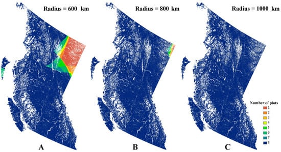
Figure 3.
The closed plots for each pixel using three search radii. Note: The search radii in (A–C) are 600 km, 800 km, and 1000 km. The number of plots in the legend indicates how many tree-ring plots are within the circle whose radii are the three lengths.
Tree-ring data from the ITRDB database include information submitted from variable projects that contribute their data to form this open-source dataset. Accordingly, the samples are from different species and times, so tree-ring data from plots varied. Tree-ring data were reviewed to ensure that they covered the study period, and if not it, they were removed prior to running the nested model across the two study periods of 1850–1889 with the 50 plots and 1890–1981 with 54.
2.3. Regression Model Selection and Validation
To reconstruct ET for each vegetated pixel, this study tested three machine-learning regressions. The independent variables and the dependent variable in the training set were the tree-ring indices (TRIs) from the plots and satellite-derived ET in that pixel from 1982 to 2010. The models tested were the random forest (RF) regression, support vector machine (SVM) regression, and convolutional neural network (CNN) regression. The most robust regression model was selected to estimate ET for both sets of tree-ring data (1850–1889 and 1890–1981).
The RF regression is a classical ensemble-learning approach using multiple decision trees in parallel whose result was the averaged values among the trees [24]. For this work, the bagging method and 100 trees for each RF regression were used [16]. The SVM regression is a sophisticated machine-learning approach which transforms input features into high-dimensional spaces to search for the maximum distance to the nearest training-data point [25]. SVM regression had a great performance on the dataset with less training samples [26] and there was a good match with our scenario where the number of training years was no more than 30. The CNN regression is a deep-learning approach with a feedforward neural network which showed an excellent performance in remote-sensing regression [27]. In our study, the max epochs, initial learning rate, and learning-rate drop factor were 100, 0.03, and 0.9, respectively.
The 5-fold cross-validation was applied to determine which model was the best, using four metrics: root mean square error (RMSE, Equation (1)), MAPE (Equation (2)), MAE (Equation (3)), and adjusted R square (Equation (4)). Those metrics were widely applied in related research [28,29]. Though Spiess and Neumeyer [30] claimed that the R square cannot fully reflect the model performances, our metrics still contain the adjusted R square due to its numerous applications in previous studies. For each validation, one year was chosen as the validation set, and another 23 or 24 years as the training set (Table 1). This study repeated the process five times, with five different validation years; calculated the metrics for each round; and then averaged them.
where S and A are the simulated ETs and actual ETs; n is the number of samples; c the number of regression coefficients; and SSE and SST are the sum of square error and the sum of squared total, respectively.

Table 1.
The training and validation scheme.
2.4. Exploring the Relationship Between the ET and Climate Factors
Annual ET maps from 1850 to 1981 were generated using the best machine-learning approach among the three. Our study then combined the simulated (1850–1981) and the real (1982–2010) into a complete dataset spanning the whole study period. For each year, the mean annual ET values were calculated within the three ecodomain boundaries.
Due to the low number of available weather stations in the Polar and Dry ecodomains, our study was only able to use one weather station for each ecodomain (Atlin in the Polar and Hedley NP Mine for the Dry ecodomain). In some years, these stations had some data missing, which could impair possible correlations between ET and climate factors in Polar and Dry ecodomains and introduce uncertainty into the analysis. The Humid Temperate ecodomain is large, and its climatic conditions are diverse, including coastal areas, inland areas, and mountainous areas, so three weather stations were chosen to reflect this variability, namely Quatsino station (coastal areas), Fort St. James station (inland areas), and Golden A station (mountainous areas). Once stations were identified, metrics for each ecodomain between 1905 and 2010 were recorded. The relationship between ET and climate factors for each ecodomain was determined by calculating correlation coefficients (r) (Equation (5)):
where xi, yi, , and are specific ET value, specific climate metric, the averaged ET value, and the averaged climate metric.
3. Results
3.1. Model Performances
Model performances were tested in two phases (1850–1889 and 1890–1980) using three models (RF, SVM, and CNN), and we identified that RF was the best among the three models (Table 2 and Figure 4). In Phase 1, the RF regression outperformed the other approaches and had the highest adjusted R2 value (0.69), the lowest RMSE (10.72 mm/month), the lowest MAPE (15.50%), and the lowest MAE (9.24 mm/month, Table 2). CNN had the worst performance, with an adjusted R2, RMSE, MAPE, and MAE of 0.24, 17.90 mm/month, 24.15%, and 14.09 mm/month, respectively. Phase 2 yielded similar results, with the RF regression outperforming the others. The RF model had an adjusted R square, RMSE, MAPE, and MAE of 0.69, 10.79 mm/month, 15.74%, and 9.39 mm/month, respectively. The CNN regression was also the poorer performer in Phase 2. There was a small difference in RF metrics between Phase 1 and 2, but they were slightly better for Phase 1, indicating that the model based on 50 plots was the best of the two.
Table 2.
Metrics of three model performances.
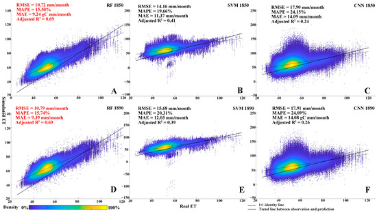
Figure 4.
Model performances of three models in two phases. Note: The six scatter plots (A–F) display the model performances in Fold 1 validation (1985). The values in the figure are the average values of five validations. Results highlighted in red show the best performance among the three approaches. RF had the best performances in both phases among the three. The x and y axes are real ET and simulated ET value, respectively.
3.2. Spatiotemporal Change in ET
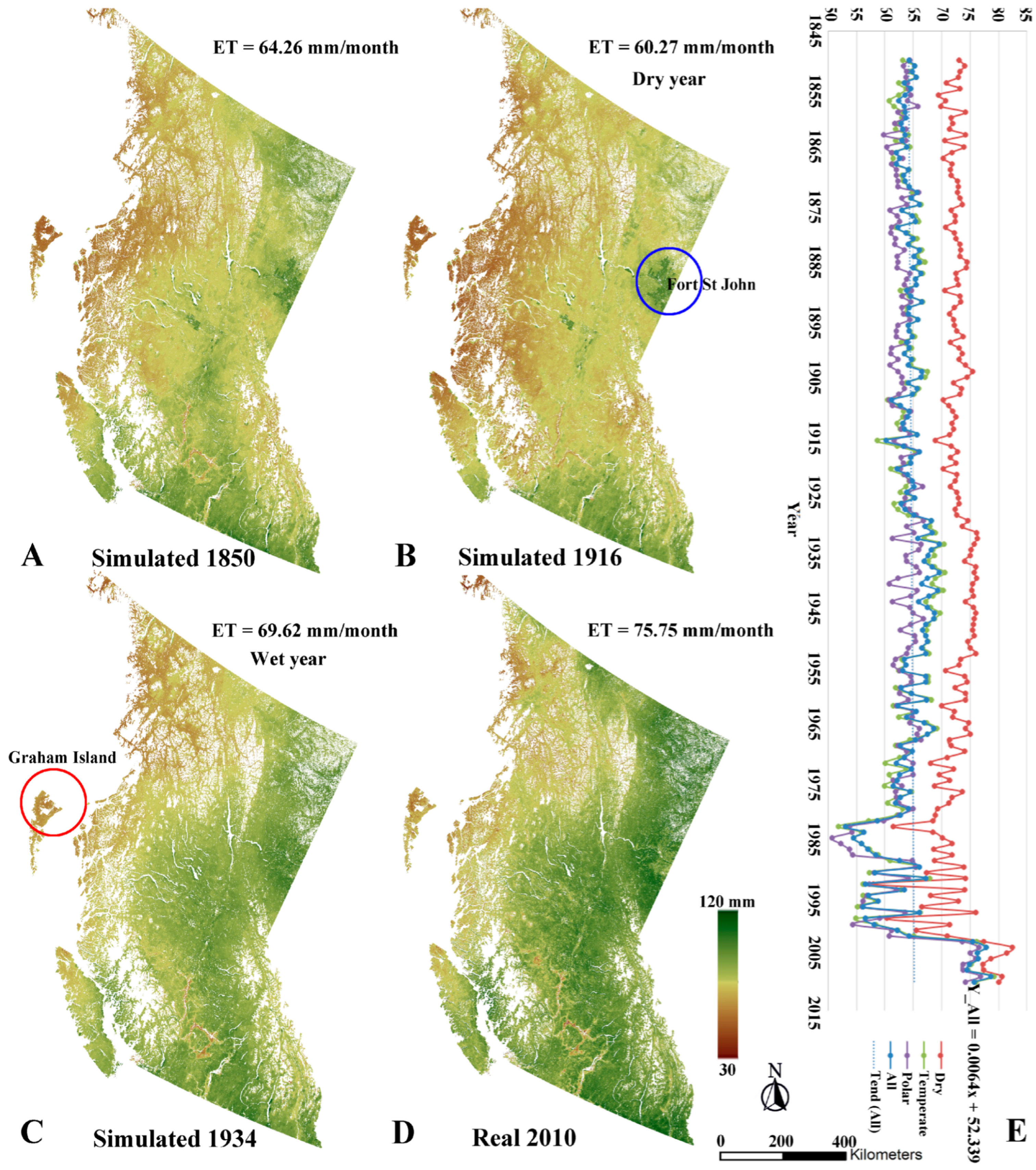
To assess spatiotemporal variation over the study period, four years were selected from the simulated ET maps (1850–1981) and satellite maps (1981–2010). These were the first and last years of record in 1850 and 2010 with a mean ET value of 64.26 mm/month and 75.75 mm/month, respectively, as well as a low ET year in 1916 at 60.27 mm/month and higher ET year of 1934, with a mean of 69.62 mm/month (Figure 5—Appendix A Figure A1 shows the simulated ET maps for every decade from 1851 to 1981). ET was increasing from 1850 to 2010, as noted by the positive value of slope for the full record (y = 0.0064x + 52.339—Figure 5E). Although there are broad provincial trends, it is important to note that there is some regional variability, as observed in 1916, when ET remained higher in Fort St. John and some other regions outside the provincial lower mean and lower ET rates at Graham Island and other northwest locations in 1934 despite the majority of the provinces having higher ET rates (Figure 5B,C).

Figure 5.
The simulated and real ET maps in 1850, 1916, 1934, and 2010. Note: The figures in (A–D) are the simulated or real ET maps of 1850, 1916, 1934, and 2010. Annual ET for the province as a whole (All) as well as the Polar, Humid Temperature, and Dry ecodomain (E) The regression between ET in whole area (Y_All) and Year (x) shows a positive relationship: Y = 0.0064x + 52.339.
3.3. ET and Climate Factors in the Three Ecodomains
ET was estimated within each provincial ecodomain for two equal time periods, namely 1850–1929 and 1931–2010. There was a general increase through the 1930s and 1950s, and there has been greater variability since the 1980s, but there have been substantial increases since the early 2000s, helping to drive the difference (Figure 5E). It was observed that ET in the Dry and Polar ecodomains were the highest and the lowest, respectively, among the three regions, regardless of the sub-period (Figure 6A). The average ET in the Dry ecodomain within the last half period reached 74.01 mm/month, while the ET in the Polar ecodomain was only 63.12 mm/month within the first half period. There were three correlations in the Humid Temperate ecodomain of note, with maximum summer temperature and mean summer temperature having a significant positive correlation (r = 0.257 and 0.318, respectively; Figure 6B), as well as a significant negative correlation between summer precipitation and ET (r = −0.208). There was also a positive but not significant correlation between maximum summer temperature and ET in the Dry ecodomain (r = 0.273, p = 0.055). The Polar ecodomain did not show any significant correlations (p > 0.05).
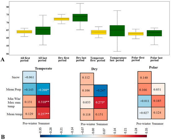
Figure 6.
The ET changes in three ecodomains and the correlations between ET and climate. Note: The ETs in the last half period are greater than the ones in the first half period for all ecodomains in (A). In (B), ET shows a positive relationship with summer temperature. **, *, and # indicate that p < 0.01, p < 0.05, and p = 0.055 in (B).
4. Discussion
4.1. RF Model Is the Best Model Among the Three
Ranking of the three machine learning approaches were consistent in both phases (1850–1889 and 1890–1981) with random forest (RF) > support vector machine (SVM) > convolutional neural network (CNN, Figure 4). The CNN had the poorest performance, which is likely due to the size of the training sample for each pixel because it was small (less than 25, Table 1). To have a good predictive accuracy, deep learning as an advanced learning model typically requires more than 150 samples [31], but the intent of this work was to draw from publicly available tree-ring data and ET remote-sensing images from 1982 to 2010, which did not meet that sample size requirement. The SVM’s performance was slightly better, as it is less sensitive to the size of the training set [32], but compared to the ensemble approach, it may have poorer accuracy. The RF, a typical ensemble machine-learning approach, generated multiple decision trees (100 trees in our study) which were trained individually. Final output was the average of 100 decision trees, which reduced both bias and variance [33], so RF was chosen as our machine-learning model to reconstruct ET from 1850 to 2010.
Contrary to our expectations, the RF in Phase 1 with 50 tree-ring plots was a little better than the one in Phase 2 with 54 plots. Two possible reasons for this finding are that the difference between the Phase 1 and Phase 2 sample size was only four plots, and the newly added plots were primarily located in Southern British Columbia, so the overall effect was small. Secondly, one of the new plots, a subalpine fir plot (Appendix A Table A1), was the only such plot among the 54. It is possible that the vegetation surrounding the subalpine fir plot exhibited different growth patterns, which could have led to poorer model performance when the additional plots were included. We suggest that future studies should carefully consider both the size of the training set and distribution of local vegetation when they choose their models to reconstruct a paleo-record with a small training set. Advanced models or deep-learning techniques may not always be superior to traditional machine-learning models depending upon data availability.
4.2. ET Increase from 1850 to 2010
Previous paleoclimate studies reconstructed ET as one single value for a whole study area. This assumes every area was similarly influenced by solar forcing and ignores the role of regional factors in driving spatial heterogeneity [34]. Zhang et al. [35] determined that regional wind, temperature, and vegetation conditions could influence ET. In 1916, one of the lowest ET years provincially, Fort St. John had high ET (blue circle in Figure 5B). Conversely, in 1934, a high provincial ET year, Graham Island (red circle in Figure 5C) had low ET. Topographic variations or the local micro-climate might be the main cause of the observed spatial heterogeneity, as has been observed elsewhere [36], but should be validated for British Columbia.
Findings indicate there has been a general increase in ET in British Columbia over the period of record, as was hypothesized, but the trend is complex. The ET in the latter half period (1931–2010) was higher than that observed in the first half (1850–1929) for all ecodomains (Figure 5E and Figure 6A). ET variability has increased since the mid-1950s and has been its most variable over the last 40 years, with the highest ET values noted between 2005 and 2015, driving a general increase over time (Figure 5E and Figure 6B). The increasing ET level and the great fluctuation might be driven by global warming and more frequent extreme weather events. Kosatsky et al. [37] identified that the extreme heat event of the summer of 2009 led to higher respiratory mortality than previous years in Vancouver, British Columbia. Others also reported that the frequency of heat events increased in British Columbia within recent decades, aligning with our findings [38,39]. In the absence of water limitations, increasing ET might benefit British Columbia vegetation, but if water scarcity and drought occurs, the outcomes may be negative. Accordingly, we suggest that ET conditions be monitored to understand the potential impact on forests and grassland to understand ecosystem resilience in the face of anticipated climate change.
4.3. Regional Effects on the ET in the Three Ecodomains
Maximum summer temperatures and mean precipitation have a strong influence on ET in British Columbia. The correlation between ET and climate factors (summer maximum temperature and monthly mean precipitation) in the Dry ecodomain was not statistically significant but was close (Figure 6B). The Humid Temperate ecodomain and Dry ecodomain share a similar story, with ET increasing under higher summer temperature and lower summer precipitation (Figure 6B). The main growing season in British Columbia is summer, and the increasing temperature-pattern changes observed might extend the growing period if water is not limiting. Lo et al. [40] identified a positive correlation between August temperature and tree-ring chronology of lodgepole pine in Kelowna, British Columbia. The Dry and Humid Temperate ecodomains have abundant summer precipitation, and the reduction in rainy days may indicate more sunshine. Warm temperatures and adequate precipitation are key factors for driving essential ecological processes [41,42,43]. The mean maximum summer temperature and ET had a moderate positive correlation in the Polar ecodomain (Figure 6B), even though the p-value did not reach a significant level. The Humid Temperate and Dry ecodomains showed a positive response in ET for summer maximum temperatures, and the former for mean summer temperature as well.
In summary, our findings highlighted that maximum temperature in summer and mean precipitation in summer had strong influences on the ET in British Columbia, where the Humid Temperate and Dry ecodomains constitute a large portion of the province.
4.4. Limitation and Future Study
There are three limitations to this study that can be improved in future work by (i) updating the model approach; (ii) increasing tree-ring and weather station data; and (iii) considering other disturbances, such as pest outbreaks. Firstly, our study only tested three models (RF, CNN, and SVM) and chose the best (RF) among them, but the RF has been shown to overfit the results if model parameters are not carefully tuned [44,45]. Secondly, future work in British Columbia and elsewhere should incorporate more regional weather station representation across topographic ranges where possible. Climate data of sufficient quality can be found within government, industry, or academic sources. In addition to climate data, it would be good to increase tree-ring data beyond that available from ITRDB to other academic and government research sources [46,47]. This study only had 54 plots, and most of plots had short periods later than 1850. Accordingly, earlier periods could not be explored, and the spatial distribution of available data was patchy, with several areas of the province having a limited number of plots. Where possible, it would also be good to broaden the spatial distribution, as well as the type of tree rings from coniferous and deciduous tree species to assess differences between them and across regions. Lastly, it would be good to bring in other factors influencing ET, such as insect disturbances and outbreaks, as well as wildfire [48,49,50]. Despite these limitations with the current analysis, the available data produced historical estimates of ET that allowed comparison across regions and time. The improved input model estimates will also improve and form a baseline for comparison to future estimates under changing climate conditions.
5. Conclusions
Our study reconstructed annual British Columbia ET maps from 1850 to 1981 using machine-learning approaches and 54 tree-ring plots. The random forest regression approach had the best performance, with fewest errors and highest accuracy. Modeled output showed there to be spatial and temporal variations across British Columbia. Although ET fluctuated, it generally increased over the period of record, especially in recent decades. There was a variable response of ET to climate factors across the three ecodomains. ET was highest in the Dry ecodomain and lowest in the Polar ecodomain. Temperature and precipitation had similar ET effects in the Humid Temperate ecodomain and Dry ecodomain, where ET was significantly and positively correlated to mean maximum summer temperature and negatively correlated with monthly mean summer precipitation. The Polar ecodomain did not display strong correlation with any climate factors. This difference in response across the three ecodomains aligns with the rationale for their designation as areas of broad climatic uniformity. The annual simulated ET maps for the past 170 years provide a unique opportunity to look at spatial and temporal variation across the landscape to compare with future projected climatic conditions to gain some insight as to how forests may respond.
Author Contributions
All authors contributed significantly to this work. Conceptualization, H.L., J.R.; methodology, H.L.; formal analysis, H.L.; writing—original draft preparation, H.L.; writing—review and editing, J.R. All authors have read and agreed to the published version of the manuscript.
Funding
This research was funded by British Columbia Ministry of Forests Research Program. And the APC was funded by British Columbia Ministry of Forests Research Program.
Data Availability Statement
The original contributions presented in the study are included in the article, further inquiries can be directed to the corresponding author.
Acknowledgments
We acknowledge the Species and Habitats Portfolio of the British Columbia Ministry of Forests Research Program that provided funding for the post-doctoral fellowship.
Conflicts of Interest
The authors declare no conflicts of interest.
Appendix A
Table A1.
Sample plot information from the ITRDB.
Table A1.
Sample plot information from the ITRDB.
| ID | ITRDB Plot Name | Species | Period 1850–1889 or Period 1890–1981 | Lat | Lon | ITRDB DOI |
|---|---|---|---|---|---|---|
| 1 | wa137 | PIPO | Period 1890–1981 | 48.7800 | −120.2700 | https://doi.org/10.25921/x9g7-8z46 |
| 2 | wa138 | PIPO | Period 1890–1981 | 48.1800 | −120.2600 | https://doi.org/10.25921/8xmk-5s78 |
| 3 | wa139 | PIPO | Period 1890–1981 | 48.5100 | −118.7500 | https://doi.org/10.25921/k6rt-kb84 |
| 4 | wa140 | PIPO | Period 1890–1981 | 48.5900 | −119.1400 | https://doi.org/10.25921/y0kg-f958 |
| 5 | wa141 | PIPO | Period 1890–1981 | 48.6000 | −119.7000 | https://doi.org/10.25921/ytpk-jj18 |
| 6 | wa143 | TSME | Period 1890–1981 | 48.8607 | −121.6850 | https://doi.org/10.25921/bxk6-be53 |
| 7 | wa145 | TSME | Period 1890–1981 | 48.5048 | −121.2088 | https://doi.org/10.25921/h1nx-5503 |
| 8 | wa146 | TSME | Period 1890–1981 | 47.8444 | −121.0359 | https://doi.org/10.25921/h0qc-1372 |
| 9 | wa148 | TSME | Period 1890–1981 | 48.6798 | −121.3227 | https://doi.org/10.25921/jz4r-sm15 |
| 10 | wa149 | PSME | Period 1890–1981 | 48.5880 | −123.1970 | https://doi.org/10.25921/1frg-zk64 |
| 11 | wa150 | CANO | Period 1890–1981 | 48.8150 | −121.9281 | https://doi.org/10.25921/j01a-m794 |
| 12 | wa151 | CANO | Period 1890–1981 | 48.0708 | −121.8103 | https://doi.org/10.25921/ybdk-x158 |
| 13 | wa152 | CANO | Period 1890–1981 | 48.8119 | −122.0361 | https://doi.org/10.25921/pf2c-qw03 |
| 14 | wa153 | TSME | Period 1890–1981 | 48.7979 | −121.8739 | https://doi.org/10.25921/5w1w-qd73 |
| 15 | wa154 | LALY | Period 1890–1981 | 48.1608 | −120.3522 | https://doi.org/10.25921/znf2-hk61 |
| 16 | wa161 | THPL | Period 1890–1981 | 48.7676 | −117.0609 | https://doi.org/10.25921/7rpk-ec27 |
| 17 | ak131 | TSME | Period 1890–1981 | 58.3833 | −134.4333 | https://doi.org/10.25921/qnyc-ex43 |
| 18 | ak150 | TSME | Period 1890–1981 | 58.7400 | −135.9800 | https://doi.org/10.25921/xwfv-gf55 |
| 19 | ak192 | CHNO | Period 1890–1981 | 58.6300 | −134.9310 | https://doi.org/10.25921/87db-m027 |
| 20 | ak193 | CHNO | Period 1890–1981 | 58.6580 | −134.9640 | https://doi.org/10.25921/cznb-x933 |
| 21 | ak195 | CHNO | Period 1890–1981 | 58.4120 | −134.5250 | https://doi.org/10.25921/9dzn-gd10 |
| 22 | ak197 | CHNO | Period 1890–1981 | 56.8320 | −133.5840 | https://doi.org/10.25921/hj2w-ev37 |
| 23 | ak198 | PICO | Period 1890–1981 | 58.4410 | −135.6090 | https://doi.org/10.25921/gna9-m858 |
| 24 | ak209 | TSME | Period 1890–1981 | 58.7400 | −135.9800 | https://doi.org/10.25921/zqx9-3t97 |
| 25 | cana590 | PCGL | Period 1890–1981 | 60.7600 | −135.7400 | https://doi.org/10.25921/wqs2-sf82 |
| 26 | cana591 | PICO | Period 1890–1981 | 60.7600 | −135.7400 | https://doi.org/10.25921/9yz1-2q87 |
| 27 | cana490 | TSME | Period 1890–1981 | 52.2800 | −126.9000 | https://doi.org/10.25921/vn0c-7h28 |
| 28 | cana469 | TSME | Period 1890–1981 | 52.2800 | −126.8900 | https://doi.org/10.25921/ze1d-4312 |
| 29 | can675 | TSME | Period 1890–1981 | 52.2900 | −126.8900 | https://doi.org/10.25921/f6ak-yk37 |
| 30 | cana476 | TSME | Period 1890–1981 | 52.2200 | −126.3400 | https://doi.org/10.25921/snpm-sr02 |
| 31 | cana467 | TSME | Period 1890–1981 | 51.2700 | −125.4300 | https://doi.org/10.25921/7tna-ek16 |
| 32 | cana646 | TSME | Period 1890–1981 | 50.5919 | −123.0172 | https://doi.org/10.25921/rctz-nf70 |
| 33 | cana645 | ABAM | Period 1890–1981 | 50.5919 | −123.0172 | https://doi.org/10.25921/z774-jr28 |
| 34 | cana641 | TSME | Period 1890–1981 | 50.3580 | −122.4875 | https://doi.org/10.25921/24rp-df66 |
| 35 | cana468 | TSME | Period 1890–1981 | 50.3500 | −122.4800 | https://doi.org/10.25921/8k3r-bs88 |
| 36 | can674 | TSME | Period 1890–1981 | 50.3500 | −122.4800 | https://doi.org/10.25921/24rp-df66 |
| 37 | can673 | TSME | Period 1890–1981 | 49.1600 | −121.6300 | https://doi.org/10.25921/gcj6-nk39 |
| 38 | cana557 | PCMA | Period 1890–1981 | 61.3080 | −121.2990 | https://doi.org/10.25921/pjfz-jw90 |
| 39 | cana643 | PIPO | Period 1890–1981 | 50.5364 | −121.2763 | https://doi.org/10.25921/k0q5-fd38 |
| 40 | can679 | PIPO | Period 1890–1981 | 50.5400 | −121.2700 | https://doi.org/10.25921/t0zq-j160 |
| 41 | can678 | PCEN | Period 1890–1981 | 50.8100 | −118.9700 | https://doi.org/10.25921/axw7-1j58 |
| 42 | can677 | PCEN | Period 1890–1981 | 51.1700 | −118.1300 | https://doi.org/10.25921/ymyd-k033 |
| 43 | can717 | PCEN | Period 1890–1981 | 49.5872 | −117.4003 | https://doi.org/10.25921/16g7-w724 |
| 44 | cana647 | PCEN | Period 1890–1981 | 52.2230 | −117.1955 | https://doi.org/10.25921/5ms4-ym52 |
| 45 | can676 | PCEN | Period 1890–1981 | 51.7100 | −116.5100 | https://doi.org/10.25921/4731-ge67 |
| 46 | cana581 | PCEN | Period 1890–1981 | 50.6100 | −115.1200 | https://doi.org/10.25921/n1jk-f831 |
| 47 | cana529 | PIAL | Period 1890–1981 | 49.7700 | −114.5300 | https://doi.org/10.25921/17r9-sf87 |
| 48 | cana528 | LALY | Period 1890–1981 | 49.3100 | −114.4300 | https://doi.org/10.25921/j0qn-qq37 |
| 49 | cana566 | PSME | Period 1890–1981 | 49.8900 | −114.3000 | https://doi.org/10.25921/z637-rn38 |
| 50 | cana583 | PSME | Period 1890–1981 | 49.8900 | −114.1800 | https://doi.org/10.25921/dp7t-w436 |
| 51 | cana464 | ABLA | Both | 50.5900 | −123.5900 | https://doi.org/10.25921/y1dm-7r82 |
| 52 | cana611 | PSME | Both | 50.8530 | −120.5200 | https://doi.org/10.25921/xn24-th08 |
| 53 | cana644 | PIPO | Both | 50.5478 | −121.2729 | https://doi.org/10.25921/94td-1252 |
| 54 | cana649 | PSME | Both | 54.6485 | −124.4300 | https://doi.org/10.25921/10c9-v582 |
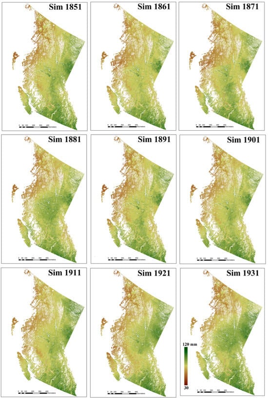

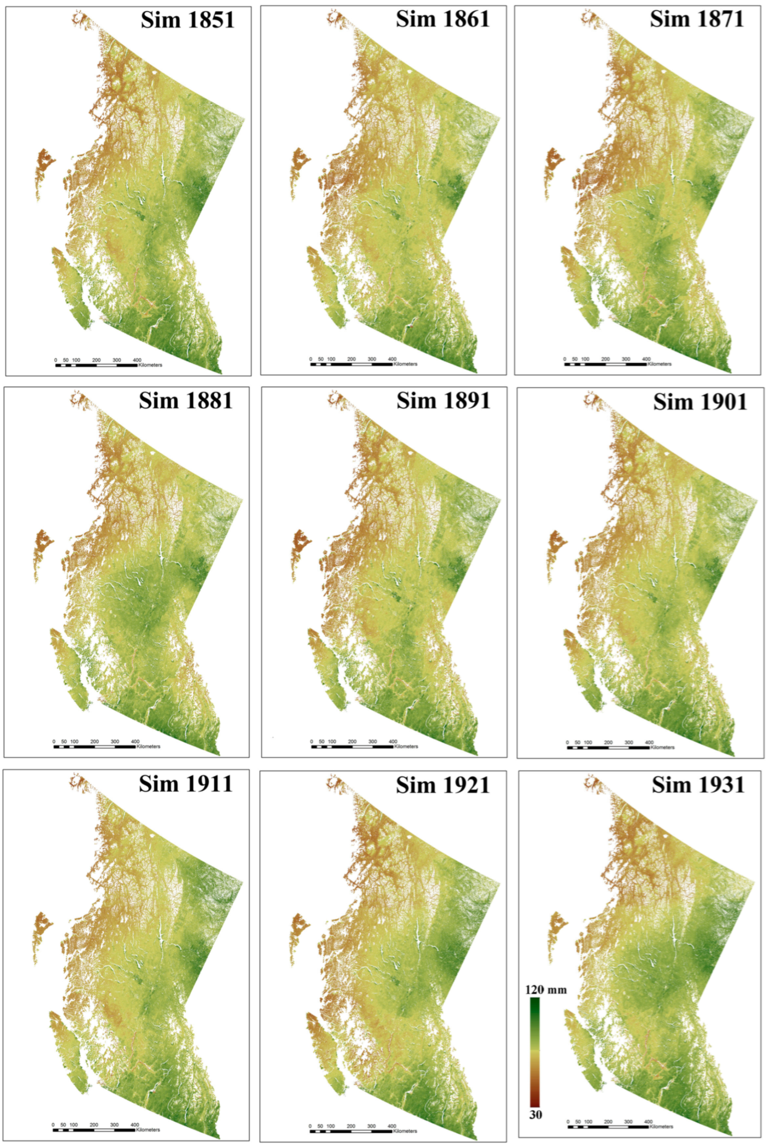
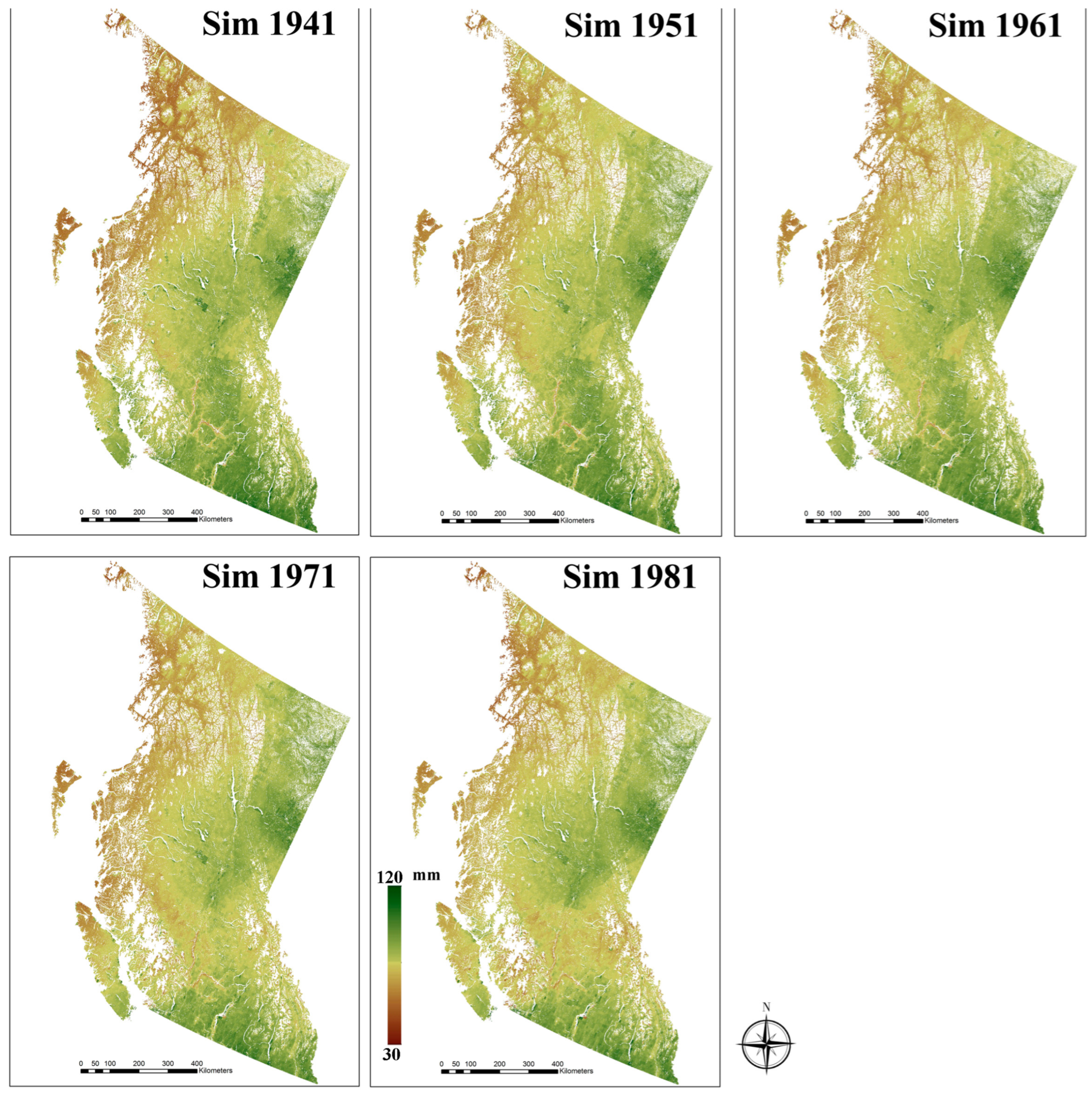
Figure A1.
The simulated ET for every decade from 1851 to 1981 (unit: mm/month).
Figure A1.
The simulated ET for every decade from 1851 to 1981 (unit: mm/month).
References
- Novák, V.; Novák, V. Evapotranspiration: A component of the water cycle. In Evapotranspiration in the Soil-Plant-Atmosphere System; Springer: Berlin/Heidelberg, Germany, 2012; pp. 1–13. [Google Scholar] [CrossRef]
- Lu, Y.; Kueppers, L. Increased heat waves with loss of irrigation in the United States. Environ. Res. Lett. 2015, 10, 064010. [Google Scholar] [CrossRef]
- Ritchie, J.T. Soil water balance and plant water stress. In Understanding Options for Agricultural Production; Springer: Dordrecht, The Netherlands, 1998; pp. 41–54. [Google Scholar] [CrossRef]
- Tan, X.; Liu, M.; Du, N.; Zwiazek, J.J. Ethylene enhances root water transport and aquaporin expression in trembling aspen (Populus tremuloides) exposed to root hypoxia. BMC Plant Biol. 2021, 21, 227. [Google Scholar] [CrossRef] [PubMed]
- Tanner, W.; Beevers, H. Transpiration, a prerequisite for long-distance transport of minerals in plants? Proc. Natl. Acad. Sci. USA 2001, 98, 9443–9447. [Google Scholar] [CrossRef] [PubMed]
- Glenn, E.P.; Huete, A.R.; Nagler, P.L.; Hirschboeck, K.K.; Brown, P. Integrating remote sensing and ground methods to estimate evapotranspiration. Crit. Rev. Plant Sci. 2007, 26, 139–168. [Google Scholar] [CrossRef]
- Alfieri, J.G.; Kustas, W.P.; Anderson, M.C. A Brief Overview of Approaches for Measuring Evapotranspiration. Agroclimatol. Link. Agric. Clim. 2020, 60, 109–127. [Google Scholar] [CrossRef]
- Zhang, Y.; Qin, H.; Zhang, J.; Hu, Y. An in-situ measurement method of evapotranspiration from typical LID facilities based on the three-temperature model. J. Hydrol. 2020, 588, 125105. [Google Scholar] [CrossRef]
- Mao, Y.; Wang, K. Comparison of evapotranspiration estimates based on the surface water balance, modified Pen-man-Monteith model, and reanalysis data sets for continental China. J. Geophys. Res. Atmos. 2017, 122, 3228–3244. [Google Scholar] [CrossRef]
- Elnashar, A.; Wang, L.; Wu, B.; Zhu, W.; Zeng, H. Synthesis of global actual evapotranspiration from 1982 to 2019. Earth Syst. Sci. Data 2021, 13, 447–480. [Google Scholar] [CrossRef]
- Senay, G.B.; Leake, S.; Nagler, P.L.; Artan, G.; Dickinson, J.; Cordova, J.T.; Glenn, E.P. Estimating basin scale evapotranspiration (ET) by water balance and remote sensing methods. Hydrol. Process. 2011, 25, 4037–4049. [Google Scholar] [CrossRef]
- Talsma, C.J.; Good, S.P.; Jimenez, C.; Martens, B.; Fisher, J.B.; Miralles, D.G.; McCabe, M.F.; Purdy, A.J. Partitioning of evapotranspiration in remote sensing-based models. Agric. For. Meteorol. 2018, 260, 131–143. [Google Scholar] [CrossRef]
- Zhou, J.; Wang, Y.; Su, B.; Wang, A.; Tao, H.; Zhai, J.; Kundzewicz, Z.W.; Jiang, T. Choice of potential evapotranspiration formulas influences drought assessment: A case study in China. Atmos. Res. 2020, 242, 104979. [Google Scholar] [CrossRef]
- Cabral-Alemán, C.; Villanueva-Díaz, J.; Quiñonez-Barraza, G.; Gómez-Guerrero, A.; Arreola-Ávila, J.G. Reconstruction of the standardized precipitation-evapotranspiration index for the Western Region of Durango State, Mexico. Forests 2022, 13, 1233. [Google Scholar] [CrossRef]
- Li, H.; Thapa, I.; Speer, J.H. Fine-scale NDVI reconstruction back to 1906 from tree-rings in the greater Yellowstone ecosystem. Forests 2021, 12, 1324. [Google Scholar] [CrossRef]
- Li, H.; Speer, J.H.; Malubeni, C.C.; Wilson, E. Reconstructing a Fine Resolution Landscape of Annual Gross Primary Product (1895–2013) with Tree-Ring Indices. Remote Sens. 2024, 16, 3744. [Google Scholar] [CrossRef]
- D’Andrea, G.; Šimůnek, V.; Castellaneta, M.; Vacek, Z.; Vacek, S.; Pericolo, O.; Zito, R.G.; Ripullone, F. Mismatch between Annual Tree-Ring Width Growth and NDVI Index in Norway Spruce Stands of Central Europe. Forests 2022, 13, 1417. [Google Scholar] [CrossRef]
- Gilani, H.R.; Innes, J.L. The state of British Columbia’s forests: A global comparison. Forests 2020, 11, 316. [Google Scholar] [CrossRef]
- Demarchi, D.A. An Introduction to the Ecoregions of British Columbia; Wildlife Branch, Ministry of Environment, Lands and Parks: Victoria, BC, USA, 1996. [Google Scholar]
- Richard, L.H.; Harold, C.F. User’s Manual for Program ARSTAN. Tree-Ring Chronologies of Western North America: California, Eastern Oregon and Northern Great Basin; University of Arizona Press: Tucson, AZ, USA, 1986; Available online: https://books.google.ca/books/about/Tree_ring_Chronologies_of_Western_North.html?id=iLwbHwAACAAJ&redir_esc=y (accessed on 5 January 2025).
- Speer, J.H. Fundamentals of Tree-Ring Research; University of Arizona Press: Tucson, AZ, USA, 2010. [Google Scholar]
- Government of Canada, Natural Resources Canada, Canada Centre for Remote Sensing. 2010 Land Cover of Canada. Natural Resources Canada, Federal Geospatial Platform. 2023. Available online: https://www.cec.org/north-american-environmental-atlas/land-cover-2010-landsat-30m/ (accessed on 5 January 2025).
- Liu, H.; Xiao, P.; Zhang, X.; Chen, S.; Wang, Y.; Wang, W. Winter snow cover influences growing-season vegetation productivity non-uniformly in the Northern Hemisphere. Commun. Earth Environ. 2023, 4, 487. [Google Scholar] [CrossRef]
- Ho, T.K. Random decision forests. In Proceedings of the 3rd International Conference on Document Analysis and Recognition, Montreal, QC, Canada, 14–16 August 1995; Volume 1, pp. 278–282. [Google Scholar] [CrossRef]
- Cortes, C.; Vapnik, V. Support-Vector Networks. Mach. Learn. 1995, 20, 273–297. [Google Scholar] [CrossRef]
- Liu, Z.; Wang, L.; Zhang, Y.; Chen, C.P. A SVM controller for the stable walking of biped robots based on small sample sizes. Appl. Soft Comput. 2016, 38, 738–753. [Google Scholar] [CrossRef]
- Chen, Z.; Liu, D.; Wan, K.; Huang, W.; Chen, N. Estimation and Spatiotemporal Analysis of Surface Evaporation in the Yangtze River Basin from 2010 to 2019. Remote Sens. 2023, 16, 57. [Google Scholar] [CrossRef]
- Liang, M.; Zhang, L.; Wu, S.; Zhu, Y.; Dai, Z.; Wang, Y.; Qi, J.; Chen, Y.; Du, Z. A high-resolution land surface temperature downscaling method based on geographically weighted neural network regression. Remote Sens. 2023, 15, 1740. [Google Scholar] [CrossRef]
- Li, H.; Thapa, I.; Xu, S.; Yang, P. Mapping the Normalized Difference Vegetation Index for the Contiguous US Since 1850 Using 391 Tree-Ring Plots. Remote Sens. 2024, 16, 3973. [Google Scholar] [CrossRef]
- Spiess, A.N.; Neumeyer, N. An evaluation of R2 as an inadequate measure for nonlinear models in pharmacological and biochemical research: A Monte Carlo approach. BMC Pharmacol. 2010, 10, 6. [Google Scholar] [CrossRef] [PubMed]
- Shahinfar, S.; Meek, P.; Falzon, G. “How many images do I need?” Understanding how sample size per class affects deep learning model performance metrics for balanced designs in autonomous wildlife monitoring. Ecol. Inform. 2020, 57, 101085. [Google Scholar] [CrossRef]
- Matykiewicz, P.; Pestian, J. Effect of small sample size on text categorization with support vector machines. In BioNLP: Proceedings of the 2012 Workshop on Biomedical Natural Language Processing; Association for Computational Linguistics: Montréal, QC, Canada, 2012; pp. 193–201. [Google Scholar]
- Webb, G.I.; Zheng, Z. Multistrategy ensemble learning: Reducing error by combining ensemble learning techniques. IEEE Trans. Knowl. Data Eng. 2004, 16, 980–991. [Google Scholar] [CrossRef]
- Shinker, J.J. Visualizing spatial heterogeneity of western US climate variability. Earth Interact. 2010, 14, 1–15. [Google Scholar] [CrossRef]
- Zhang, Y.; He, T.; Liang, S.; Zhao, Z. A framework for estimating actual evapotranspiration through spatial heterogeneity-based machine learning approaches. Agric. Water Manag. 2023, 289, 108499. [Google Scholar] [CrossRef]
- McVicar, T.R.; Van Niel, T.G.; Li, L.; Hutchinson, M.F.; Mu, X.; Liu, Z. Spatially distributing monthly reference evapotranspiration and pan evaporation considering topographic influences. J. Hydrol. 2007, 338, 196–220. [Google Scholar] [CrossRef]
- Kosatsky, T.; Henderson, S.B.; Pollock, S.L. Shifts in mortality during a hot weather event in Vancouver, British Columbia: Rapid assessment with case-only analysis. Am. J. Public Health 2012, 102, 2367–2371. [Google Scholar] [CrossRef]
- Long-term Change in Air Temperature in B.C. (1900–2013) (July 2015). Available online: https://www2.gov.bc.ca/gov/content/environment/research-monitoring-reporting/reporting/environmental-reporting-bc/climate-change-indicators?keyword=2016 (accessed on 5 January 2025).
- Lee, M.J.; McLean, K.E.; Kuo, M.; Richardson, G.R.; Henderson, S.B. Chronic diseases associated with mortality in British Columbia, Canada during the 2021 western North America extreme heat event. GeoHealth 2023, 7, e2022GH000729. [Google Scholar] [CrossRef]
- Lo, Y.H.; Blanco, J.A.; Seely, B.; Welham, C.; Kimmins, J.H. Relationships between climate and tree radial growth in interior British Columbia, Canada. For. Ecol. Manag. 2010, 259, 932–942. [Google Scholar] [CrossRef]
- Xu, Z.; Shimizu, H.; Ito, S.; Yagasaki, Y.; Zou, C.; Zhou, G.; Zheng, Y. Effects of elevated CO2, warming and precipitation change on plant growth, photosynthesis and peroxidation in dominant species from North China grassland. Planta 2014, 239, 421–435. [Google Scholar] [CrossRef]
- Hui, D.; Yu, C.L.; Deng, Q.; Dzantor, E.K.; Zhou, S.; Dennis, S.; Luo, Y. Effects of precipitation changes on switchgrass photosynthesis, growth, and biomass: A mesocosm experiment. PLoS ONE 2018, 13, e0192555. [Google Scholar] [CrossRef] [PubMed]
- Baribault, T.W.; Kobe, R.K.; Finley, A.O. Tropical tree growth is correlated with soil phosphorus, potassium, and calcium, though not for legumes. Ecol. Monogr. 2012, 82, 189–203. [Google Scholar] [CrossRef]
- Bearup, L.A.; Maxwell, R.M.; Clow, D.W.; McCray, J.E. Hydrological effects of forest transpiration loss in bark beetle-impacted watersheds. Nat. Clim. Change 2014, 4, 481–486. [Google Scholar] [CrossRef]
- Erbeli, F.; He, K.; Cheek, C.; Rice, M.; Qian, X. Exploring the machine learning paradigm in determining risk for reading disability. Sci. Stud. Read. 2023, 27, 5–20. [Google Scholar] [CrossRef]
- Halabaku, E.; Bytyçi, E. Overfitting in Machine Learning: A Comparative Analysis of Decision Trees and Random Forests. Intell. Autom. Soft Comput. 2024, 39, 5–20. [Google Scholar] [CrossRef]
- Creasman, P.P.; Bannister, B.; Towner, R.H.; Dean, J.S.; Leavitt, S.W. Reflections on the foundation, persistence, and growth of the Laboratory of Tree-Ring Research, circa 1930–1960. Tree-Ring Res. 2012, 68, 81–89. [Google Scholar] [CrossRef]
- Guiterman, C.H.; Gille, E.; Shepherd, E.; McNeill, S.; Payne, C.R.; Morrill, C. The international tree-ring Data Bank at fifty: Status of stewardship for future scientific discovery. Tree-Ring Res. 2024, 80, 13–18. [Google Scholar] [CrossRef]
- Niccoli, F.; Pacheco-Solana, A.; Delzon, S.; Kabala, J.P.; Asgharinia, S.; Castaldi, S.; Valentini, R.; Battipaglia, G. Effects of wildfire on growth, transpiration and hydraulic properties of Pinus pinaster Aiton forest. Dendrochronologia 2023, 79, 126086. [Google Scholar] [CrossRef]
- Szatniewska, J.; Zavadilova, I.; Nezval, O.; Krejza, J.; Petrik, P.; Čater, M.; Stojanović, M. Species-specific growth and transpiration response to changing environmental conditions in floodplain forest. For. Ecol. Manag. 2022, 516, 120248. [Google Scholar] [CrossRef]


Disclaimer/Publisher’s Note: The statements, opinions and data contained in all publications are solely those of the individual author(s) and contributor(s) and not of MDPI and/or the editor(s). MDPI and/or the editor(s) disclaim responsibility for any injury to people or property resulting from any ideas, methods, instructions or products referred to in the content. |
© 2025 by the authors. Licensee MDPI, Basel, Switzerland. This article is an open access article distributed under the terms and conditions of the Creative Commons Attribution (CC BY) license (https://creativecommons.org/licenses/by/4.0/).