
Flood Mapping and Assessment of Crop Damage Based on Multi-Source Remote Sensing: A Case Study of the “7.27” Rainstorm in Hebei Province, China


 , ,
, ,  and
and
Abstract
1. Introduction
2. Materials
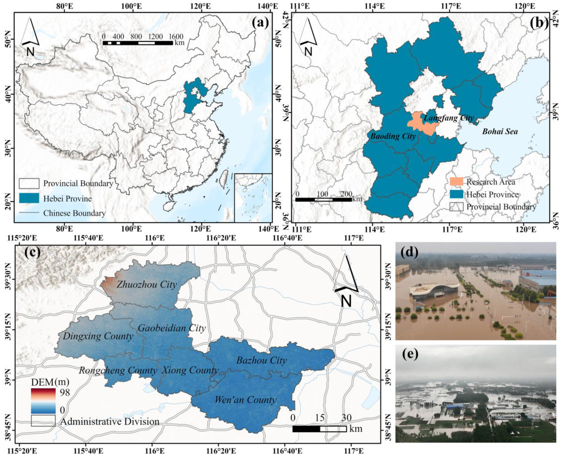
2.1. Study Areas
2.2. Data and Processing
2.2.1. SAR Data
2.2.2. Optical Data
- (1)
- GF-6 PMS
- (2)
- Landsat-8 OLI
2.2.3. Other Data
- (1)
- Sentinel-2 MSI: Sentinel-2 imagery was used to produce maximum synthetic NDVI values of crops before and after the flood, aiding in crop damage classification and assessment. The Sentinel-2 imagery, produced by the European Space Agency (ESA), contains 13 spectral bands. This study used the red (band 4) and near-infrared (band 8) bands with a resolution of 10 m.
- (2)
- DEM data: DEM data from the Shuttle Radar Topography Mapping Mission (SRTM) with a resolution of 30 m were used to mask mountainous regions in the northwestern part of the study area, avoiding confusion between mountain shadows and water bodies.
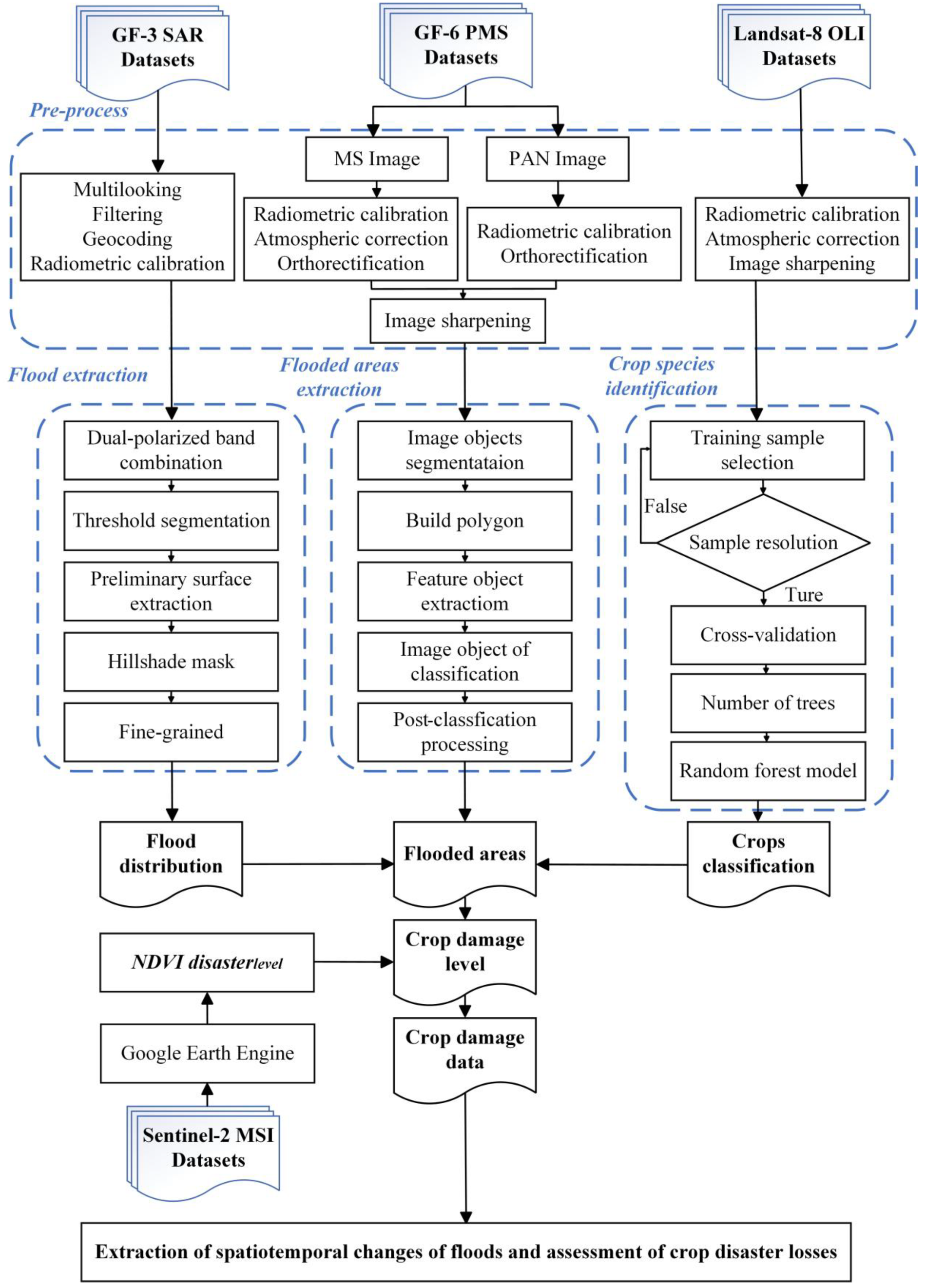
3. Methodology
3.1. SAR Image Flood Recognition
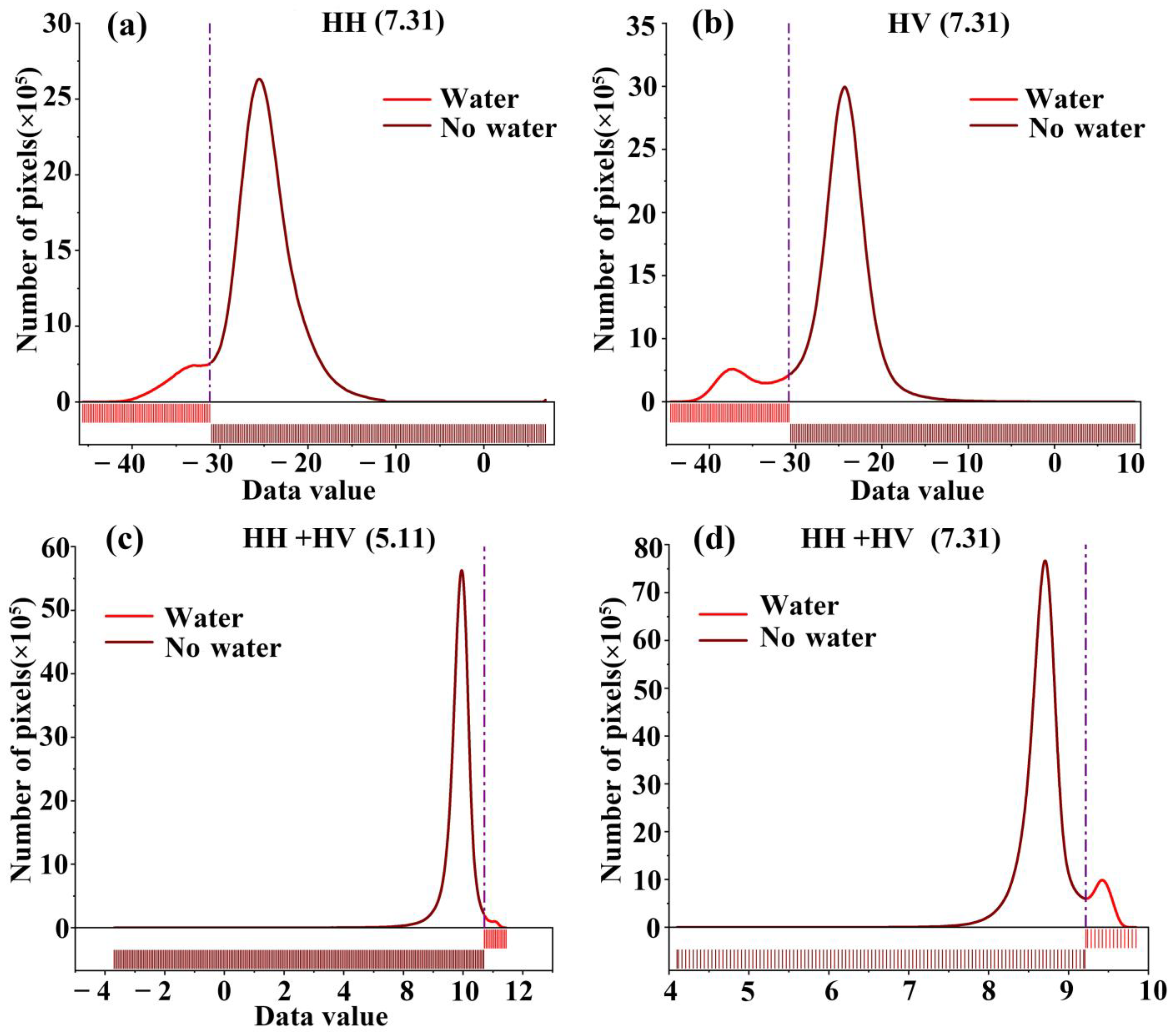
3.1.1. SAR Image Band Combination
3.1.2. Delineation of Critical Thresholds
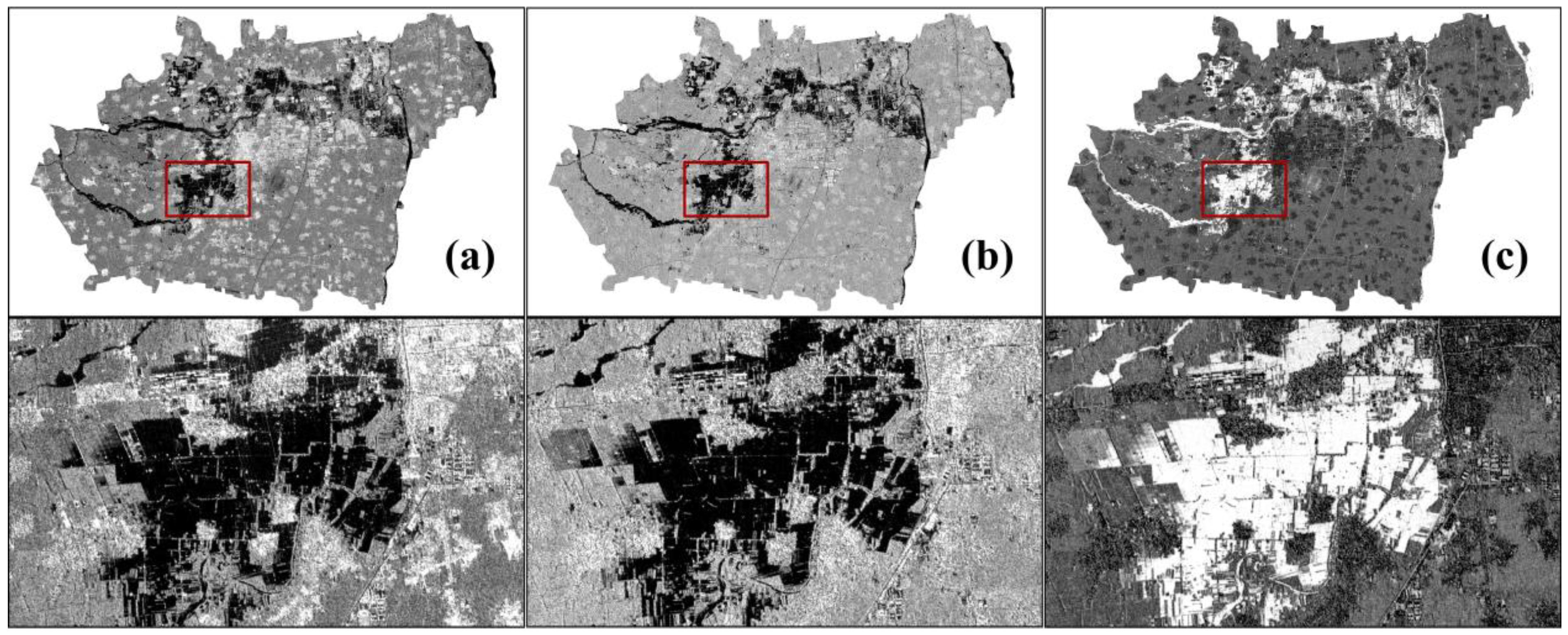
3.1.3. Combined Image Accuracy
3.2. Optical Image Flooding Area Mapping
3.2.1. Object-Oriented Sample Construction
3.2.2. Sample Classifier Selection
3.3. Crop Classification
3.4. Crop Damage Classification
4. Results
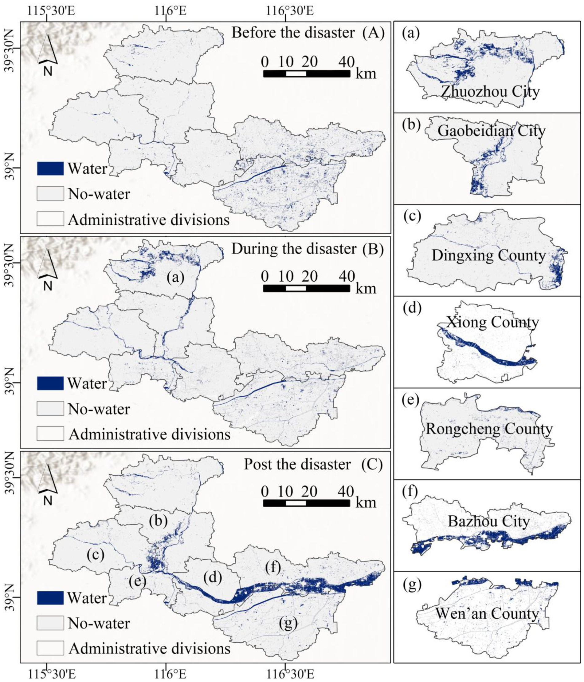
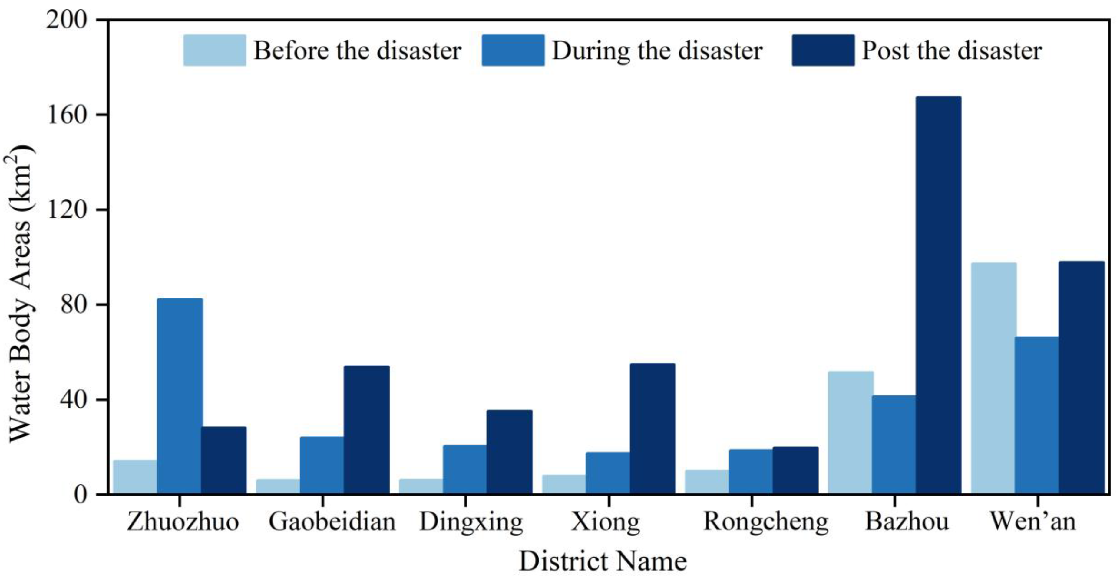
4.1. Spatiotemporal Pattern of Water Body Areas
4.2. Flood Inundation Areas
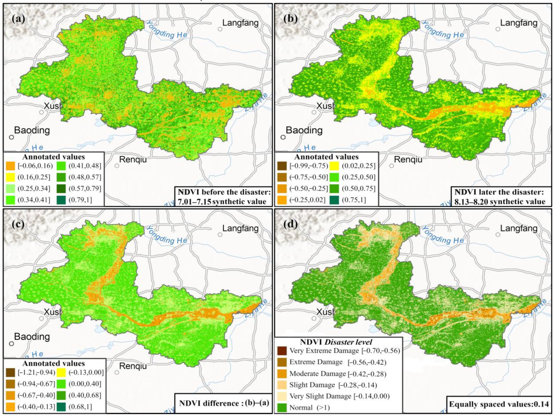
4.3. Crop Damage Assessment
4.3.1. Crop Classification Results
4.3.2. Damage Classification Results
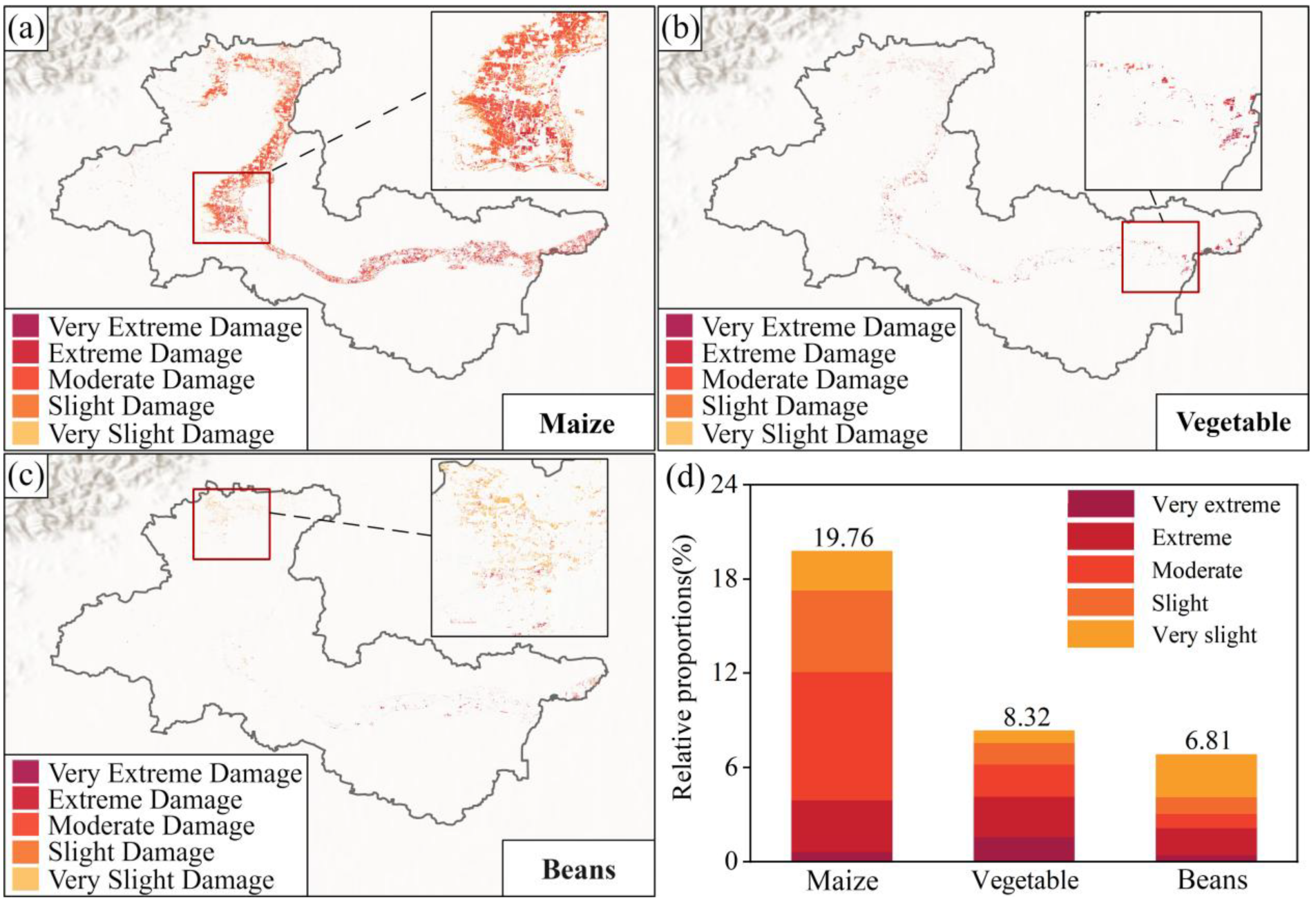
4.3.3. Damage Assessment Results
5. Discussion
5.1. Challenges and Recommendations
5.2. Result Validation and Uncertainty Analysis
6. Conclusions
Supplementary Materials
Author Contributions
Funding
Data Availability Statement
Conflicts of Interest
References
- Zhang, Y.; Wang, Y.; Chen, Y.; Liang, F.; Liu, H. Assessment of future flash flood inundations in coastal regions under climate change scenarios—A case study of Hadahe River basin in northeastern China. Sci. Total Environ. 2019, 693, 133550. [Google Scholar] [CrossRef] [PubMed]
- Chen, T.-L.; Lin, Z.-H. Planning for climate change: Evaluating the changing patterns of flood vulnerability in a case study in New Taipei City, Taiwan. Stoch. Environ. Res. Risk Assess. 2020, 35, 1161–1174. [Google Scholar] [CrossRef]
- Kuang, D.; Liao, K.H. Learning from floods: Linking flood experience and flood resilience. J. Environ. Manag. 2020, 271, 111025. [Google Scholar] [CrossRef] [PubMed]
- Jonkman, S.N. Global perspectives on loss of human life caused by floods. Nat. Hazards 2005, 34, 151–175. [Google Scholar] [CrossRef]
- Rentschler, J.; Salhab, M.; Jafino, B.A. Flood exposure and poverty in 188 countries. Nat. Commun. 2022, 13, 3527. [Google Scholar] [CrossRef]
- Wang, K.; Yang, Y.; Reniers, G.; Huang, Q. A study into the spatiotemporal distribution of typhoon storm surge disasters in China. Nat. Hazards 2021, 108, 1237–1256. [Google Scholar] [CrossRef]
- Zhou, C.; Chen, P.; Yang, S.; Zheng, F.; Yu, H.; Tang, J.; Lu, Y.; Chen, G.; Lu, X.; Zhang, X.; et al. The impact of Typhoon Lekima (2019) on East China: A postevent survey in Wenzhou City and Taizhou City. Front. Earth Sci. 2021, 16, 109–120. [Google Scholar] [CrossRef]
- Lan, Q.; Dong, J.; Lai, S.; Wang, N.; Zhang, L.; Liao, M. Flood inundation extraction and its impact on ground subsidence using Sentinel-1 data: A case study of the “7.20” rainstorm event in Henan Province, China. IEEE J. Sel. Top. Appl. Earth Obs. Remote Sens. 2024, 17, 2927–2938. [Google Scholar] [CrossRef]
- Piao, S.; Ciais, P.; Huang, Y.; Shen, Z.; Peng, S.; Li, J.; Zhou, L.; Liu, H.; Ma, Y.; Ding, Y.; et al. The impacts of climate change on water resources and agriculture in China. Nature 2010, 467, 43–51. [Google Scholar] [CrossRef]
- Wang, Y.-J.; Gao, C.; Zhai, J.-Q.; Li, X.-C.; Su, B.-D.; Hartmann, H. Spatio-temporal changes of exposure and vulnerability to floods in China. Adv. Clim. Change Res. 2014, 5, 197–205. [Google Scholar] [CrossRef]
- Shi, J.; Cui, L.; Tian, Z. Spatial and temporal distribution and trend in flood and drought disasters in East China. Environ. Res. 2020, 185, 109406. [Google Scholar] [CrossRef] [PubMed]
- Zhou, J.; Yu, H.; Ren, Y.; Yang, Y.; Liu, X.; Chen, G.; Ma, Z.; Zhao, W.; Chen, S.; Wei, Y.; et al. Remote effects of double typhoons on record-breaking rainfall: A case study in North China. Atmos. Res. 2024, 304, 107377. [Google Scholar] [CrossRef]
- Zhang, M.; Liu, D.; Wang, S.; Xiang, H.; Zhang, W. Multisource Remote Sensing Data-Based Flood Monitoring and Crop Damage Assessment: A Case Study on the 20 July 2021 Extraordinary Rainfall Event in Henan, China. Remote Sens. 2022, 14, 5771. [Google Scholar] [CrossRef]
- Rahman, M.S.; Di, L.; Yu, E.; Lin, L.; Yu, Z. Remote Sensing Based Rapid Assessment of Flood Crop Damage Using Novel Disaster Vegetation Damage Index (DVDI). Int. J. Disaster Risk Sci. 2020, 12, 90–110. [Google Scholar] [CrossRef]
- Qamer, F.M.; Abbas, S.; Ahmad, B.; Hussain, A.; Salman, A.; Muhammad, S.; Nawaz, M.; Shrestha, S.; Iqbal, B.; Thapa, S. A framework for multi-sensor satellite data to evaluate crop production losses: The case study of 2022 Pakistan floods. Sci. Rep. 2023, 13, 4240. [Google Scholar] [CrossRef]
- Singha, M.; Dong, J.; Sarmah, S.; You, N.; Zhou, Y.; Zhang, G.; Doughty, R.; Xiao, X. Identifying Floods and Flood-Affected Paddy Rice Fields in Bangladesh Based on Sentinel-1 Imagery and Google Earth Engine. ISPRS J. Photogramm. Remote Sens. 2020, 166, 278–293. [Google Scholar] [CrossRef]
- Quan, T.; Zhang, C.; Feng, Y.; Li, H.; Guo, Y.; Shen, Y. Impact of the “23·7” Extreme Heavy Precipitation on Maize Yield in the Hebei Plain. Chin. J. Eco-Agric. 2024, 32, 1023–1032. [Google Scholar] [CrossRef]
- Liu, M.; Jin, S.; Gu, C.; Li, J.; Li, S.; Liu, L. Chinese Satellite-Based Flood Mapping and Damage Assessment in Dongdian Flood Detention Basin, China. J. Resour. Ecol. 2024, 15, 1344–1357. [Google Scholar] [CrossRef]
- Shrestha, R.; Di, L.; Yu, E.G.; Kang, L.; Shao, Y.-Z.; Bai, Y.-Q. Regression model to estimate flood impact on corn yield using MODIS NDVI and USDA cropland data layer. J. Integr. Agric. 2017, 16, 398–407. [Google Scholar] [CrossRef]
- Shen, X.; Anagnostou, E.N.; Allen, G.H.; Brakenridge, R.; Kettner, A.J. Near-real-time non-obstructed flood inundation mapping using synthetic aperture radar. Remote Sens. Environ. 2019, 221, 302–315. [Google Scholar] [CrossRef]
- Wang, Z.; Wang, X.; Li, G.; Wu, W.; Liu, Y.; Song, Z.; Song, H. Historical information fusion of dense multi-source satellite image time series for flood extent mapping. Inf. Fusion. 2024, 109, 102445. [Google Scholar] [CrossRef]
- Huang, C.; Chen, Y.; Zhang, S.; Wu, J. Detecting, extracting, and monitoring surface water from space using optical sensors: A review. Rev. Geophys. 2018, 56, 333–360. [Google Scholar] [CrossRef]
- Khan, S.I.; Hong, Y.; Wang, J.; Yilmaz, K.K.; Gourley, J.J.; Adler, R.F.; Brakenridge, G.R.; Policelli, F.; Habib, S.; Irwin, D. Satellite remote sensing and hydrologic modeling for flood inundation mapping in Lake Victoria Basin: Implications for hydrologic prediction in ungauged basins. IEEE Trans. Geosci. Remote Sens. 2011, 49, 85–95. [Google Scholar] [CrossRef]
- Cian, F.; Marconcini, M.; Ceccato, P. Normalized difference flood index for rapid flood mapping: Taking advantage of EO big data. Remote Sens. Environ. 2018, 209, 712–730. [Google Scholar] [CrossRef]
- Tsokas, A.; Rysz, M.; Pardalos, P.M.; Dipple, K. SAR data applications in earth observation: An overview. Expert Syst. Appl. 2022, 205, 117342. [Google Scholar] [CrossRef]
- Bentivoglio, R.; Isufi, E.; Jonkman, S.N.; Taormina, R. Deep learning methods for flood mapping: A review of existing applications and future research directions. Hydrol. Earth Syst. Sci. 2022, 26, 4345–4378. [Google Scholar] [CrossRef]
- Liang, J.; Liu, D. A local thresholding approach to flood water delineation using Sentinel-1 SAR imagery. ISPRS J. Photogramm. Remote Sens. 2020, 159, 53–62. [Google Scholar] [CrossRef]
- Peng, B.; Huang, Q.; Vongkusolkit, J.; Gao, S.; Wright, D.B.; Fang, Z.N.; Qiang, Y. Urban Flood Mapping with Bitemporal Multispectral Imagery Via a Self-Supervised Learning Framework. IEEE J. Sel. Top. Appl. Earth Obs. Remote Sens. 2021, 14, 2001–2016. [Google Scholar] [CrossRef]
- Sharifi, A. Flood Mapping Using Relevance Vector Machine and SAR Data: A Case Study from Aqqala, Iran. J. Indian Soc. Remote Sens. 2020, 48, 1289–1296. [Google Scholar] [CrossRef]
- Huang, X.; Xie, C.; Fang, X.; Zhang, L. Combining Pixel- and Object-Based Machine Learning for Identification of Water-Body Types from Urban High-Resolution Remote-Sensing Imagery. IEEE J. Sel. Top. Appl. Earth Obs. Remote Sens. 2015, 8, 2097–2110. [Google Scholar] [CrossRef]
- Li, M.; Wu, P.; Wang, B.; Park, H.; Hui, Y.; Yanlan, W. A Deep Learning Method of Water Body Extraction from High Resolution Remote Sensing Images with Multisensors. IEEE J. Sel. Top. Appl. Earth Obs. Remote Sens. 2021, 14, 3120–3132. [Google Scholar] [CrossRef]
- Saha, K.; Wells, N.A.; Munro-Stasiuk, M. An object-oriented approach to automated landform mapping: A case study of drumlins. Comput. Geosci. 2011, 37, 1324–1336. [Google Scholar] [CrossRef]
- Xing, K.; Cui, N.; Wang, Z.; Yu, Z.; Yu, F. A TLRTV Dual-band SAR Image Denoise-Fusion Strategy and Its Preliminary Experiment Analysis in Multi-band Airborne Radar System. IEEE J. Sel. Top. Appl. Earth Obs. Remote Sens. 2024, 17, 12031–12047. [Google Scholar] [CrossRef]
- Zhai, K.; Wu, X.; Qin, Y.; Du, P. Comparison of surface water extraction performances of different classic water indices using OLI and TM imageries in different situations. Geo-Spat. Inf. Sci. 2015, 18, 32–42. [Google Scholar] [CrossRef]
- Song, L.; Song, C.; Luo, S.; Chen, T.; Liu, K.; Li, Y.; Jing, H.; Xu, J. Refining and densifying the water inundation area and storage estimates of Poyang Lake by integrating Sentinel-1/2 and bathymetry data. Int. J. Appl. Earth Obs. Geoinf. 2021, 105, 102601. [Google Scholar] [CrossRef]
- Linhui, L.; Weipeng, J.; Huihui, W. Extracting the Forest Type from Remote Sensing Images by Random Forest. IEEE Sens. J. 2021, 21, 17447–17454. [Google Scholar] [CrossRef]
- Tong, X.; Luo, X.; Liu, S.; Xie, H.; Chao, W.; Liu, S.; Liu, S.; Makhinov, A.N.; Makhinova, A.F.; Jiang, Y. An approach for flood monitoring by the combined use of Landsat 8 optical imagery and COSMO-SkyMed radar imagery. ISPRS J. Photogramm. Remote Sens. 2018, 136, 144–153. [Google Scholar] [CrossRef]
- Di, L.; Yu, E.G.; Kang, L.; Shrestha, R.; Bai, Y.-q. RF-CLASS: A remote-sensing-based flood crop loss assessment cyber-service system for supporting crop statistics and insurance decision-making. J. Integr. Agric. 2017, 16, 408–423. [Google Scholar] [CrossRef]
- Lehner, B.; Verdin, K.; Jarvis, A. New Global Hydrography Derived from Spaceborne Elevation Data. Eos Trans. Am. Geophys. Union. 2008, 89, 93–94. [Google Scholar] [CrossRef]
- Landuyt, L.; Van Wesemael, A.; Schumann, G.J.P.; Hostache, R.; Verhoest, N.E.C.; Van Coillie, F.M.B. Flood Mapping Based on Synthetic Aperture Radar: An Assessment of Established Approaches. IEEE Trans. Geosci. Remote Sens. 2018, 57, 722–739. [Google Scholar] [CrossRef]
- Xu, B.; Li, X.; Hou, W.; Wang, Y.; Wei, Y. A Similarity-Based Ranking Method for Hyperspectral Band Selection. IEEE Trans. Geosci. Remote Sens. 2021, 59, 9585–9599. [Google Scholar] [CrossRef]
- Tapia-Silva, F.-O.; Itzerott, S.; Foerster, S.; Kuhlmann, B.; Kreibich, H. Estimation of flood losses to agricultural crops using remote sensing. Phys. Chem. Earth Parts A/B/C 2011, 36, 253–265. [Google Scholar] [CrossRef]
- Ma, Y.; Cui, Y.; Tan, H.; Wang, H. Case study: Diagnosing China’s prevailing urban flooding—Causes, challenges, and solutions. J. Flood Risk Manag. 2022, 15, e12822. [Google Scholar] [CrossRef]
- Zou, B.; Xu, X.; Zhang, L. Object-Based Classification of PolSAR Images Based on Spatial and Semantic Features. IEEE J. Sel. Top. Appl. Earth Obs. Remote Sens. 2020, 13, 609–619. [Google Scholar] [CrossRef]
- Liu, Y.; Xie, Z.; Liu, H. An Adaptive and Robust Edge Detection Method based on Edge Proportion Statistics. IEEE Trans. Image Process. 2020, 29, 5206–5215. [Google Scholar] [CrossRef]
- Wang, Y.; Qi, Q.; Jiang, L.; Liu, Y. Hybrid Remote Sensing Image Segmentation Considering Intrasegment Homogeneity and Intersegment Heterogeneity. IEEE Geosci. Remote Sens. Lett. 2020, 17, 22–26. [Google Scholar] [CrossRef]
- Imani, M.; Ghassemian, H. An overview on spectral and spatial information fusion for hyperspectral image classification: Current trends and challenges. Inf. Fusion 2020, 59, 59–83. [Google Scholar] [CrossRef]
- Caldera, H.J.; Wirasinghe, S.J.N.h. A universal severity classification for natural disasters. Nat. Hazards 2022, 111, 1533–1573. [Google Scholar] [CrossRef]
- He, B.; Huang, X.; Ma, M.; Chang, Q.; Tu, Y.; Li, Q.; Zhang, K.; Hong, Y. Analysis of flash flood disaster characteristics in China from 2011 to 2015. Nat. Hazards 2017, 90, 407–420. [Google Scholar] [CrossRef]
- Huang, X.; Chan, J.C.L.; Zhan, R.; Yu, Z.; Wan, R. Record-breaking rainfall accumulations in eastern China produced by Typhoon In-fa (2021). Atmos. Sci. Lett. 2023, 24, e1153. [Google Scholar] [CrossRef]


| Data | Period | Resolution | Source | Purpose of This Study |
|---|---|---|---|---|
| GF-3 SAR data | 11 May 2023/31 July 2023/1 August 2023/6 August 2023/7 August 2023 | 10 m | http://ids.ceode.ac.cn/gfds/gflogin (accessed on 7 September 2023) | Flood extent extraction |
| GF-6 PMS data | 15 August 2023/19 August 2023/23 August 2023 | 8 m | http://ids.ceode.ac.cn/gfds/gflogin (accessed on 7 September 2023) | Inundation area identification |
| Landsat-8 OLI data | 19 July 2023 | 15 m | United States Geological Survey | Crop classification |
| Sentinel-2 MSI data | 1 July 2023–15 July 2023/13 August 2023–20 August 2023 | 10 m | Google Earth Engine | Crop disaster assessment |
| SRTM DEM data | 2007 | 30 m | Google Earth Engine | To mask the hilly terrains |
| Classifier | Overall Accuracy | Kappa Coefficient |
|---|---|---|
| KNN | 89.13% | 0.85 |
| PCA | 83.74% | 0.78 |
| SVM | 95.65% | 0.94 |
| Community | Corps Cultivated Area/Hectare (ha) | |||
|---|---|---|---|---|
| Maize | Beans | Vegetables | Bare-Land | |
| Zhuozhou City | 25,915 | 6264 | 10,369 | 2581 |
| Gaobeidian City | 29,807 | 3247 | 8182 | 3024 |
| Dingxing County | 37,875 | 4565 | 6920 | 2328 |
| Rongcheng County | 10,517 | 1584 | 2461 | 3782 |
| Xiong County | 14,646 | 7038 | 6834 | 4694 |
| Bazhou County | 16,336 | 9808 | 9352 | 10,686 |
| Wen’an County | 35,317 | 8173 | 7388 | 18,351 |
Disclaimer/Publisher’s Note: The statements, opinions and data contained in all publications are solely those of the individual author(s) and contributor(s) and not of MDPI and/or the editor(s). MDPI and/or the editor(s) disclaim responsibility for any injury to people or property resulting from any ideas, methods, instructions or products referred to in the content. |
© 2025 by the authors. Licensee MDPI, Basel, Switzerland. This article is an open access article distributed under the terms and conditions of the Creative Commons Attribution (CC BY) license (https://creativecommons.org/licenses/by/4.0/).
Share and Cite
Wen, C.; Sun, Z.; Li, H.; Han, Y.; Gunasekera, D.; Chen, Y.; Zhang, H.; Zhao, X. Flood Mapping and Assessment of Crop Damage Based on Multi-Source Remote Sensing: A Case Study of the “7.27” Rainstorm in Hebei Province, China. Remote Sens. 2025, 17, 904. https://doi.org/10.3390/rs17050904
Wen C, Sun Z, Li H, Han Y, Gunasekera D, Chen Y, Zhang H, Zhao X. Flood Mapping and Assessment of Crop Damage Based on Multi-Source Remote Sensing: A Case Study of the “7.27” Rainstorm in Hebei Province, China. Remote Sensing. 2025; 17(5):904. https://doi.org/10.3390/rs17050904
Chicago/Turabian StyleWen, Chenhao, Zhongchang Sun, Hongwei Li, Youmei Han, Dinoo Gunasekera, Yu Chen, Hongsheng Zhang, and Xiayu Zhao. 2025. "Flood Mapping and Assessment of Crop Damage Based on Multi-Source Remote Sensing: A Case Study of the “7.27” Rainstorm in Hebei Province, China" Remote Sensing 17, no. 5: 904. https://doi.org/10.3390/rs17050904
APA StyleWen, C., Sun, Z., Li, H., Han, Y., Gunasekera, D., Chen, Y., Zhang, H., & Zhao, X. (2025). Flood Mapping and Assessment of Crop Damage Based on Multi-Source Remote Sensing: A Case Study of the “7.27” Rainstorm in Hebei Province, China. Remote Sensing, 17(5), 904. https://doi.org/10.3390/rs17050904