Article

An Effective Quantification of Methane Point-Source Emissions with the Multi-Level Matched Filter from Hyperspectral Imagery

1
Key Laboratory of Remote Sensing and Digital Earth, Aerospace Information Research Institute, Chinese Academy of Sciences, Beijing 100049, China
2
University of Chinese Academy of Sciences, Beijing 100049, China
*
Author to whom correspondence should be addressed.
Remote Sens. 2025, 17(5), 843; https://doi.org/10.3390/rs17050843
Submission received: 28 January 2025 / Revised: 19 February 2025 / Accepted: 26 February 2025 / Published: 27 February 2025

Abstract

:
Methane is a potent greenhouse gas that significantly contributes to global warming, making the accurate quantification of methane emissions essential for climate change mitigation. The traditional matched filter (MF) algorithm, commonly used to derive methane enhancement from hyperspectral satellite data, is limited by its tendency to underestimate methane plumes, especially at higher concentrations. To address this limitation, we proposed a novel approach—the multi-level matched filter (MLMF)—which incorporates unit absorption spectra matching using a radiance look-up table (LUT) and applies piecewise regressions for concentrations above specific thresholds. This methodology offers a more precise distinction between background and plume pixels, reducing noise interference and mitigating the underestimation of high-concentration emissions. The effectiveness of the MLMF was validated through a series of tests, including simulated data tests and controlled release experiments using satellite observations. These validations demonstrated significant improvements in accuracy: In radiance residual tests, relative errors at high concentrations were reduced from up to −30% to within ±5%, and regression slopes improved from 0.89 to 1.00. In simulated data, the MLMF reduced root mean square error (RMSE) from 1563.63 ppm·m to 337.09 ppm·m, and R² values improved from 0.91 to 0.98 for Gaussian plumes. In controlled release experiments, the MLMF significantly enhanced emission rate estimation, improving R 2 from 0.71 to 0.96 and reducing RMSE from 92.32 kg/h to 16.10 kg/h. By improving the accuracy of methane detection and emission quantification, the MLMF presents a significant advancement in methane monitoring technologies. The MLMF’s superior accuracy in detecting high-concentration methane plumes enables better identification and quantification of major emission sources. Its compatibility with other techniques and its potential for integration into real-time operational monitoring systems further extend its applicability in supporting evidence-based climate policy development and mitigation strategies.

1. Introduction

Methane ( CH 4 ) is a powerful greenhouse gas that plays a major role in global climate change. CH 4 concentration in the atmosphere has increased significantly to 1.9 ppm [1], nearly triple as much as before the industrial era, and methane is responsible for about 0.6  °C global warming [2]. Although methane is less abundant in the atmosphere than carbon dioxide ( CO 2 ), it is far more effective at trapping heat, with a warming effect more than 25 times stronger than CO 2 over a 100-year period [3], making methane a crucial factor in understanding and mitigating climate change. What further distinguishes methane is its relatively short atmospheric lifetime of about 12 years [4,5]. This means that reducing methane emissions can lead to near-term improvements in climate conditions [6], offering an effective and immediate path to slow global warming while addressing long-term environmental challenges.
Methane influences our atmosphere and climate in several important ways. In addition to contributing to the greenhouse effect, it participates in photochemical reactions that lead to the production of ground-level ozone [7], a pollutant detrimental to both human health and ecosystems. Over time, the balance of methane sources has shifted significantly. Human activities now release more methane than natural sources, leading to faster increases in atmospheric methane levels. This rapid rise has sparked serious concerns about its effects on global temperatures and weather patterns. Among all human activities contributing to emissions, the fossil fuel industry, especially oil and gas fields and coal mining, accounts for approximately 35% of global anthropogenic methane emissions [8]. A significant portion of emissions from these activities comes from point sources [9,10], which exhibit heavy-tailed distributions (i.e., a small amount of emitters contribute to a huge fraction of the total CH 4 emissions) [11]. Rapid and accurate identification and quantification of these point-source emissions are crucial for achieving methane reduction and recovery.
The timing of methane reduction efforts is crucial for fighting climate change. Methane’s short atmospheric lifespan allows for quick climate response following emissions reductions, making methane an ideal target for near-term climate mitigation. To implement these efforts effectively, reliable technical methods to identify and quantify emission sources are an urgent requirement. Satellite-based remote sensing has emerged as a critical tool due to its capacity for large-scale monitoring and high spatial and temporal resolution [12,13,14].
Modern satellites equipped with hyperspectral imaging sensors have proven especially effective for methane monitoring [15,16,17]. These sensors are capable of detecting the unique spectral absorption features of methane in the atmosphere, enabling the accurate identification, monitoring, and quantification of methane plumes from point sources such as oil and gas facilities [18,19], coal mines [20], and landfills [21]. These advanced systems can measure radiance at a fine spectral interval, allowing them to detect the unique methane absorption in the atmosphere. This technology helps scientists accurately find, monitor, and measure methane plumes coming from specific locations on Earth, providing valuable information for managing methane’s impact on climate.
Currently, two main categories of methods have been used to detect and quantify methane emissions from point sources: full-physical algorithms [22,23,24] and data-driven approaches [25,26]. Among the latter, the matched filter (MF) method has gained significant popularity. Originally developed for measuring methane emissions from aircraft [11,15,27], the MF algorithm has since been adapted for satellite-based applications [28,29,30]. It works by comparing the radiance observed by satellites with known patterns of methane absorption, effectively picking out methane signals from background noise. This method has proven especially effective with high-resolution satellite images, making it possible to detect even small sources of methane emissions with good accuracy. Using a first-order Taylor expansion to model the radiance attenuation and a linear approximation of methane absorption characteristics, this method derives methane concentration enhancement ( Δ XCH 4 ) relative to the atmospheric methane concentration.
However, the linear estimation can lead to inaccuracies, particularly underestimations, when attempting to retrieve methane concentrations from stronger plumes [31]. Many studies have focused on improving the MF algorithm to enhance its accuracy and efficiency in methane concentration retrieval. Foote et al. [26] introduced the incorporation of sparsity and an albedo correction, which enhanced the MF algorithm’s ability to retrieve methane concentrations more accurately. To address the underestimation issue of methane concentrations, further strategies have been explored. One such approach is the transformation of data into logarithmic space, which can improve the quantification of methane, especially when high variability in concentration is present. The iterative lognormal matched filter (ILMF) proposed in [32] reduces underestimation errors and improves retrieval accuracy, as demonstrated in both simulated and real-world applications, making it a more reliable tool for methane emission quantification. Furthermore, other researches have focused on further optimizing the MF algorithm by adjusting or combining the retrieval windows used in the retrieval process. These adjustments aim to enhance the accuracy of methane concentration retrievals, particularly in challenging real-world scenarios. For instance, one key development involves extending the spectral range utilized in the matched filter. By expanding the retrieval window to cover a broader spectral range (1000–2500 nm) [33], researchers have been able to significantly reduce retrieval artifacts and background noise that often complicate methane plume detection in real-world data. This enhancement is especially beneficial in the energy sector, where detecting methane emissions from point sources, such as oil and gas extraction sites, is crucial for effective monitoring.
In this study, we present an improved method, the multi-level matched filter (MLMF), to address the limitations of the original MF algorithm. By incorporating a piecewise regression approach, the MLMF algorithm aims to enhance the accuracy of methane plume quantification, particularly for point sources with high methane concentrations. Specifically, we evaluate the MLMF performance through a multi-step framework: (1) application to idealized simulated satellite measurements to validate the method under controlled conditions, (2) testing on satellite image data with overlaid simulated methane plumes of varying intensities and types, (3) analysis of real satellite observations obtained during a controlled methane release experiment. The results demonstrate that the MLMF significantly outperforms the MF approach, particularly in accurately quantifying high-emission methane sources that conventional methods commonly underestimate.

2. Materials and Methods

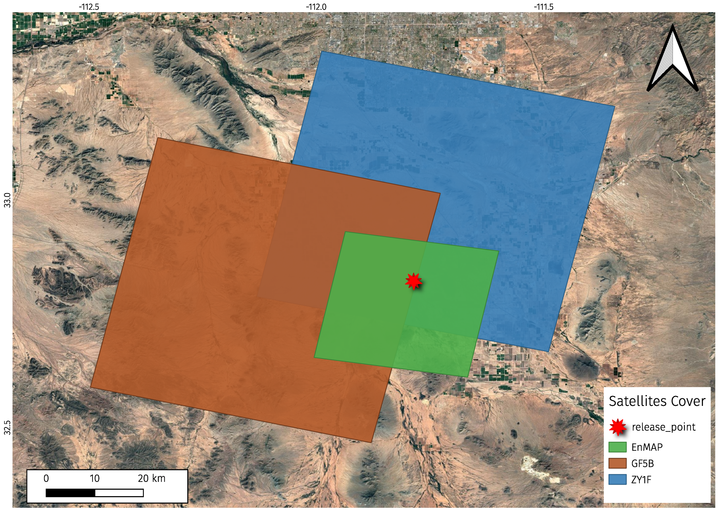
2.1. Controlled Release Experiment

Between 20 October and 30 November, 2022, a controlled methane release experiment was conducted by Stanford University to evaluate the performance and precision of satellite-based methane detection and quantification systems [34]. This single-blind test involved nine distinct satellite platforms, tasked with detecting and quantifying methane emissions under varying release rates.
Of the nine satellites, overpass observation data from three were successfully collected and utilized for analysis due to their spatial coverage and compatibility with the research objectives:
  • Gaofen-5B: One scene acquired on 15 November 2022;
  • Ziyuan-1F: One scene acquired on 26 October 2022;
  • EnMAP: One scene acquired on 7 November 2022.
Data from other platforms were excluded for the following reasons. Commercial systems such as GHGSat and WorldView-3 were inaccessible due to licensing constraints [16,35]. The HJ-2B satellite recorded only a single measurement during the experiment period, but this overpass did not coincide with active methane releases due to a communication issue. Furthermore, while publicly accessible satellites such as Sentinel-2 and Landsat 8/9 provide multispectral imagery, their sensors are not optimized for methane detection using matched-filter-like algorithms. The spatial coverage of the satellite data employed is shown in Figure 1, where the location of the methane release stacks is marked with a star symbol for clarity. The precise coordinates of the release point are at [ 32 . 8218205 , − 111 . 7857730 ].

2.2. Hyperspectral Instruments

Hyperspectral instruments, characterized by their high spectral resolution and signal-to-noise ratio (SNR), are capable of accurately deriving methane concentrations from radiance cubes [36]. These instruments measure solar radiation reflected from the Earth’s surface across hundreds of spectral bins, spanning wavelengths from 400 nm to 2500 nm. With a spatial resolution of approximately 30 m and a spectral resolution of about 8 nm, such sensors can effectively detect methane absorption features in the radiance spectrum. By leveraging methane’s absorption characteristics in the shortwave infrared (SWIR) region, concentrations above background levels can be effectively retrieved.
The satellite sensors utilized in this study are detailed in Table 1. The Advanced HyperSpectral Imager (AHSI) [30,37], onboard the Chinese satellites Gaofen5B and Ziyuan1F, is a profound instrument designed for hyperspectral imaging. It covers a spectral range from the VNIS to the SWIR spectrum, with a fine spatial resolution of 30 m and an excellent spectral resolution of approximately 8 nm [38]. Gaofen-5B, launched on 7 September 2021, and Ziyuan-1F, launched on 26 December 2021, both play significant roles in environmental monitoring and resource surveying. Several studies have validated AHSI’s capability in detecting and quantifying methane emissions from anthropogenic sources [30,39].
In addition, the Environmental Mapping and Analysis Program (EnMAP), a German hyperspectral imaging satellite, was also employed in this study. Launched in 2022, aboard a Space X Falcon 9 rocket, EnMAP primarily focuses on global-scale Earth observation and environmental assessment. It features a spatial resolution of 30 m, a swath width of 30 km, and a spectral resolution of around 8 nm. Compared to similar international hyperspectral sensors, EnMAP offers superior spectral resolution and a higher SNR, making it exceptional for detecting methane plumes from oil and gas facilities and landfills with high precision [40].

2.3. Method

2.3.1. Multi-Level Matched Filter

The matched filter algorithm is widely used and efficient for retrieving methane emissions from hyperspectral radiance data [26,28,41]. At the core of the MF method lies the principle of leveraging the distinctive absorption features of methane in the shortwave infrared (SWIR) region. This method hinges on its ability to detect subtle methane signatures within a noisy background, utilizing the unique spectral characteristics of methane absorption. The original method assumes that the recorded data contain noise following a multivariate Gaussian distribution, with mean 0 and covariance matrix Σ  [42]. According to the Beer–Lambert law, the methane absorption causes an exponentially decaying effect on radiance as its concentration increases, and after a first-order Taylor expansion, the relationship can be written linearly, which can be expressed as below:
I = I 0 e α s
I = I 0 ( 1 α s )
where I is the expected at-sensor radiance, I 0 is the expected at-sensor radiance, α represents the enhanced concentration of CH 4 due to emission activities, and  s , which is the unit absorption spectrum (UAS), characterizes the methane absorption properties for each satellite band. Mathematically, the MF method estimates the enhancement of column-averaged methane concentration enhancement by minimizing the residuals between observed spectra and a background spectrum modulated by the methane absorption effect. Since the true background radiation spectrum and the noise covariance matrix in satellite observations for the region are unknown, we approximate the background radiance, μ , using the mean of the observed spectrum [43]. Then, by calculating the difference between the observed spectrum and this approximation, we estimate the covariance matrix, Σ , for each pixel and average the covariance matrices across all pixels:
μ = 1 N i = 1 N I i
Σ = 1 N i N ( I i μ ) ( I i μ ) T .
where i denotes the pixel index and N represents the total number of pixels. The MF method operates by correlating observed spectral data with a pre-defined target spectrum, t , which represents the expected radiative transfer signal change caused by methane absorption. The radiance-dependent target spectrum, showing the spectral absorption characteristic for each band, is calculated as the element-wise multiplication of unit absorption spectrum, s , and background radiance, μ :
t s ( μ ) = μ s
Finally, the optimal estimation of methane concentration for each pixel can be deducted by solving the maximum likelihood estimation:
α ^ i = arg min α i i = 1 N ( I i μ + α i t ( μ ) ) T Σ 1 μ + α i t ( μ ) )
α ^ i = ( I i μ ) Σ 1 t T t Σ 1 t T
By applying this equation, the MF method effectively separates the methane signal from the background noise. For methane detection, the 2300 nm window is typically selected due to its strong absorption features. The specific spectral range used in this study is 2150–2500 nm across all instruments. While the 1600 nm window generally offers higher SNR [40] due to higher radiance levels, the methane absorption in the chosen window is stronger, making it more suitable for our purposes.
A key advantage of the MF method is its computational efficiency, enabling the rapid processing of large volumes of satellite data. However, the method has a notable challenge of the occurrence of false positives, where methane plumes remain undetected due to noise or retrieval artifacts. Additionally, due to its first-order linear approximation of the exponential absorption relationship, the MF method tends to underestimate emission rates, particularly for pixels with high methane concentrations. This systematic underestimation leads to the inaccurate assessment of methane plume magnitude and overall methane quantification.
Given these issues, the multi-level matched filter was proposed in this study to achieve more precise methane concentration retrieval and emission quantification. The core idea of the MLMF is to employ sequential first-order linear approximations to better capture the exponential absorption features. After the initial methane enhancement estimation, pixels are classified into two groups: background pixels with no obvious methane enhancement and potential methane plume pixels. We set a threshold of 1000 ppm·m to reduce background pixel noise. For potential methane plume pixels, the MLMF proceeds at different background concentration levels, calculating the relative methane concentration above each level.
The MLMF algorithm primarily updates two parameters: the background spectrum and the target spectrum. For each retrieval interval with index j, the background spectrum is updated by assuming uniform methane concentration enhancement, τ j , across the region. Based on a specific unit absorption spectrum, s τ j , from the pre-defined radiance look-up table (LUT) through linear regression of methane absorption effects across the enhancement region, the target spectrum for each retrieval level is also updated:
μ τ j = μ T τ j
t τ j = μ τ j s τ j
where μ τ j is the background spectrum for current retrieval level and  T τ j is the transmittance spectrum obtained from the radiance LUT. For methane concentration enhancements within an interval with a minimum of τ j , the concentration can be calculated as follows:
α ^ i _ τ j = ( I i μ τ j ) Σ 1 t τ j T t τ j Σ 1 t τ j + τ j
It is worth noting that the initial background spectrum, μ , requires refinement as it simply uses the mean of the radiance cube, which includes methane enhancement absorption pixels in the estimation. This error affects both the target spectrum and covariance matrix, ultimately influencing methane retrieval values. To address this contamination, we implement an iterative matched filter approach based on [44] that improves background spectrum and covariance estimation by subtracting methane absorption from the radiance cube using previous retrieval results. For each iteration with index k, the background spectrum, μ k , and covariance matrix, Σ k , are updated as:
μ k = 1 N i = 1 N I i α i k 1 t μ k 1
Σ k = 1 N i N d k ( d k ) T .
d k = I i ( μ k + α i k 1 t ( μ k ) )
In the MLMF algorithm, we maintain the covariance matrix identical across all retrieval levels, since the noise in different spectral bands should remain relatively stable under varying methane concentrations. While processing the entire observation area as a single unit, the estimation of background spectra and covariance can be affected by variations in detector radiometric performance along the across-track direction. To address this, we adopt a column-wise approach for the MLMF algorithm [25]. Although the calculation procedure remains identical for each column of radiance observations, this approach could lead to sparse covariance matrices due to insufficient data volume. Therefore, in this study, we process the column-wise matched filter in units of 5 columns.
The MLMF algorithm uses fixed concentration intervals, with an initial segmentation threshold of 1000 ppm·m, to achieve precise background pixel estimation. This approach helps mitigate the overestimation of methane concentrations for low-concentration pixels that can occur when fitting the unit absorption spectrum across a broad range of methane enhancements, while effectively suppressing background noise. Below 5000 ppm·m, the interval increment is set to 2000 ppm·m; above this threshold, it increases to 5000 ppm·m. The choice of those parameters was obtained through multiple trials and represents empirically derived values that provide a good balance between computational efficiency and result accuracy. To reduce computational load, the MLMF algorithm is applied only to pixels whose concentration estimates from the previous iteration fall within the current interval. For each concentration interval, we construct a unit absorption spectrum using radiance LUT to capture the specific methane absorption characteristics. This spectrum is fitted across the range from the current interval threshold to the next interval threshold, and then used for subsequent calculations. A detailed description of this methodology follows in the next section.

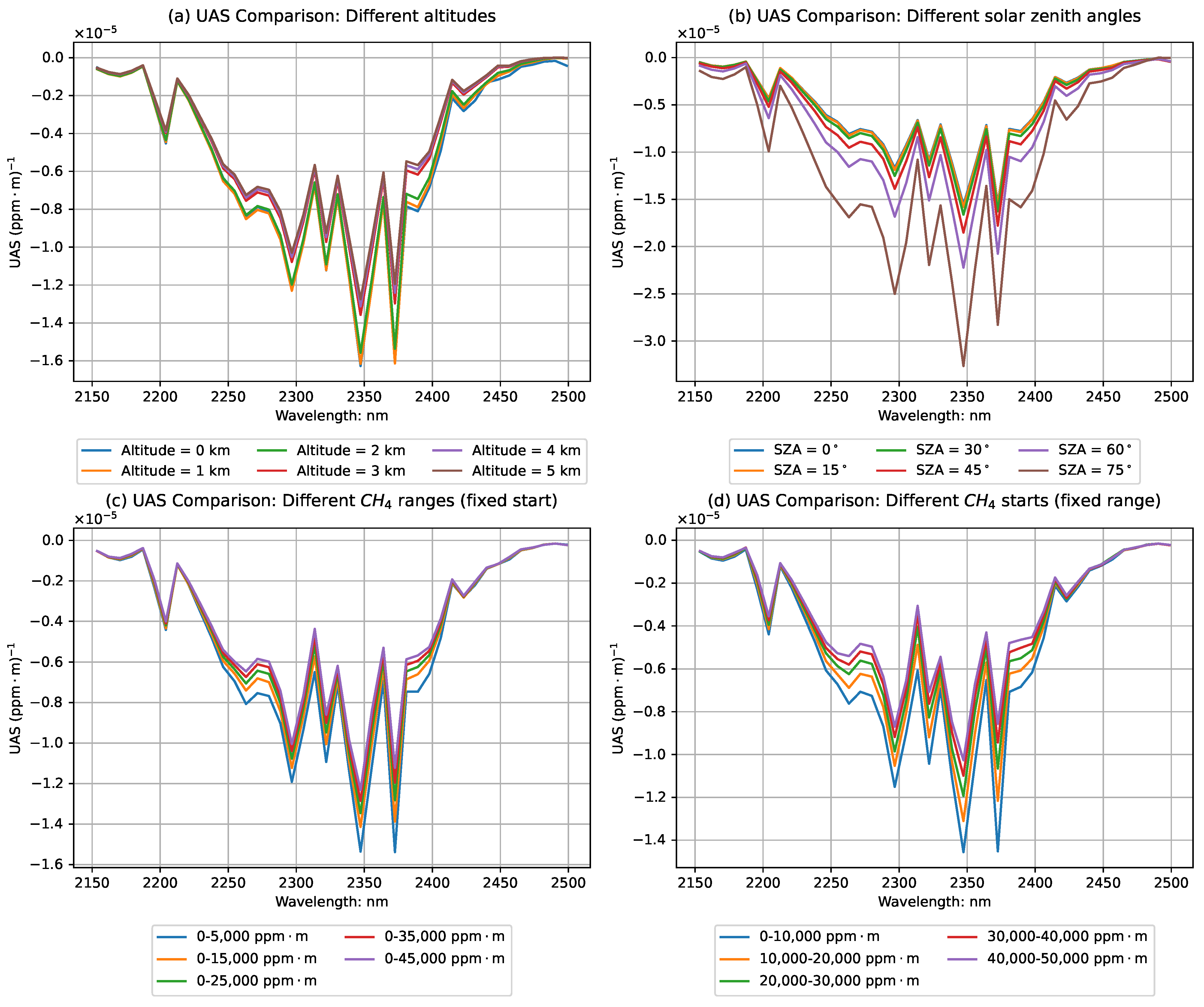
2.3.2. Unit Absorption Spectrum Construction Based on LUT

The target spectrum is an important parameter in the MF algorithm, and it can typically be obtained as the methane absorption spectrum [25] or the transmittance spectrum [45] based on radiative transfer simulations. In addition, the unit absorption spectrum has been introduced to achieve an accurate estimation of methane concentration enhancement. This spectrum characterizes the proportional change in radiance after passing through a unit path length with a unit concentration of methane enhancement, showing the absorptive characteristic of methane across different bands in the retrieval window. Generally, the unit absorption spectrum is obtained by radiative transfer simulations.
To optimize methane concentration retrieval for each observation, it is necessary to construct a unit absorption spectrum specific to the local conditions and observational geometry [41]. What is more, the MLMF algorithm requires specific unit absorption spectra for different inversion intervals, making a dynamically adaptive construction process essential. However, obtaining methane unit absorption spectra that match the current satellite image spectral channels and inversion interval through fully simulated radiative transfer models demands extensive computational resources and is not feasible for ready-to-use algorithms. Each imagery requires individual simulations based on observation geometry and other parameters.
To address this challenge, this study used MODTRAN (MODerate resolution atmospheric TRANsmission) [46] simulations to establish a radiance LUT for each different satellite sensor. This pre-generated LUT eliminates the need for real-time unit absorption spectrum simulations for future images. We set the baseline methane concentration to 1900 ppb [47] and added uniform enhancements to the atmospheric profile within 500 m of the surface [26]. Both upward and downward methane absorption paths were considered, with enhancements ranging from 0 to 50,000 ppm·m in 500 ppm·m increments. Additionally, solar azimuth angles ranging from 0° to 90° in 5° increments and surface elevations from 0 to 5 km in 1 km increments were included in the LUT. Since the study focuses on spaceborne sensors, of which the sensor height typically exceeds MODTRAN’s maximum atmospheric profile height of 120 km, sensor height was excluded from the LUT construction. Other absorbing gases were set to default values; the atmospheric model was specified as mid-latitude summer and the aerosol model was set to “no cloud or aerosol” with a visibility of 23 km. Using the center wavelength and full width at half maximum (FWHM) of hyperspectral satellite sensors, the simulated at-sensor radiance was convolved into the spectral channels of the hyperspectral satellite sensor [48].
Based on the radiance LUT, methane concentration enhancement ranges, solar altitude angles, and surface elevation parameters were specified to extract the radiance data needed for unit absorption spectrum calculations. For each spectral band, the natural logarithm of radiance under varying methane concentrations was linearly fitted against the concentration enhancement range. The slope of the best-fit line represents the unit absorption value for the current band. Figure 2 shows unit absorption spectra obtained from the radiance look-up table under different setting parameters of the radiative transfer simulation.

2.3.3. Detection and Quantification of Methane Plumes

Based on the retrieved Δ XCH 4 data from hyperspectral satellite observations, methane plumes are identified following a general procedure. Due to significant background noise caused by the multivariate Gaussian assumption and numerous retrieval artifacts exhibiting methane-like spectral characteristics, implementing a fully automated methane plume detection and masking method remains challenging. As a result, the current approach relies largely on visual inspection.
To determine a real methane emission plume, several criteria must be met. First, the concentration distribution of methane should exhibit a clear correlation with the wind direction; plumes that fail to meet this condition are excluded. Second, there must be a plausible methane source located beneath the identified plume, such as a coal mine, an oil extraction facility, like pipelines or compressor stations [49], or a landfill site. By combining wind direction data with high-resolution satellite imagery, such as those available from Google Earth, we can reliably confirm the presence of methane plumes.
To quantify point-source emission flux rates from methane plumes, there are methods that include the Gaussian plume inversion method [50], the source pixel method [14], the cross-sectional flux (CSF) method [51], and the integrated mass enhancement (IME) method [52,53]. Successful methods for point-source quantification include the CSF and IME methods, both widely applied in satellite observations, that produce consistent results. The IME method is selected in this study due to its reduced sensitivity to wind direction, incorporation of turbulent diffusion effects, and better suitability for weak wind conditions favorable for plume detection, which is calculated as:
IME = k i = 1 n p α ^ ( i )
where n p is the total number of pixels in the methane plume, α ^ ( i ) is the Δ XCH 4 of the plume pixel, and k is a scaling factor to convert the methane concentration enhancement in ppm·m into mass units, such as kg. Then, the emission flux rate can be calculated as:
Q = I M E · U e f f L p l u m e
where U e f f is the effective wind speed during the propagation of the methane plume and L is the plume length in meters. U e f f is adjusted from 10 m wind speed, U 10 . In this research, we use the same slope and intercept of the linear relation between these two parameters, which is
U e f f = 1.1 l o g U 10 + 0.6
The U 10 data are calculated by the 10 m wind U component and V component from ERA5 (fifth generation ECMWF reanalysis for global climate and weather) reanalysis data. For each plume, the nearest wind speed data in both time and location are selected. The time window is extended by one hour before and after the chosen time, while the wind-affected region is defined as a 3 × 3 grid centered on the selected position. The average wind speed within this region is calculated for subsequent analysis, and the standard deviation is used to estimate the wind speed uncertainty. The uncertainty of the emission rate estimation is calculated by an error propagation pattern proposed by [54]. Wind speed uncertainty is the dominant error contributor. The error of IME is calculated by the 1 σ methane retrieval standard deviation and the number of pixels in the methane plume. Quadratically combining the wind speed uncertainty with the standard error of the IME, the final Q random error is generated.

3. Results

3.1. Matched Filter Variants Comparison

To evaluate the performance of the MLMF, we designed an experiment using a radiance spectrum simulation dataset. The experiment was conducted assuming a sensor height of 100 km, an altitude of 0 km, a view zenith angle (VZA) of 0 , and a solar zenith angle (SZA) of 25 , along with different methane column concentrations; a total of 101 radiance spectra were simulated using varying methane column concentrations. The radiance spectrum corresponding to a methane concentration of 1900 ppb was used as the reference spectrum, which is fixed as the background spectrum in the algorithms. The remaining 100 solar radiation spectra, with methane concentrations incrementally increased by 500 ppm·m incrementally from the background level, were sequentially utilized for algorithm comparison.
Since the methane concentration enhancements were pre-defined in the simulated dataset, ideal observations of radiance in the SWIR retrieval windows were generated without considering instrument noise and spectral convolution. Additionally, uniform concentrations of the other trace gases, such as H 2 O or CO 2 , were assumed to avoid interference with methane retrieval result. Based on the known methane concentration enhancements, the results retrieved by the two algorithms are shown in Figure 3. Figure 3 illustrates the performance comparison between the MF and the proposed MLMF algorithm in a simulated scenario with randomly enhanced methane concentrations, spanning a range of 0–20,000 ppm·m. The left subplot presents the retrieval results for the MF, while the right subplot shows the MLMF performance.
When assessing bias, the MLMF demonstrates notable improvements over the traditional approach, as corroborated by Figure 3. The relative bias shown in Figure 3a consistently approaches zero across the concentration range for the MLMF, an indication of its reliable performance even under varying methane concentration scenarios. In comparison, the MF shows increasing divergence from zero, particularly at higher concentrations, highlighting its susceptibility to inaccuracies when detecting substantial methane plumes. Similarly, the absolute bias shown in Figure 3b demonstrates that the MLMF had a significantly lower absolute bias, remaining within a tight range around zero across the full enhancement scale, while the MF method displays a steadily increasing absolute bias, reaching values exceeding −2000 ppm·m at the highest true enhancements. This indicates the MLMF’s robustness in providing unbiased methane retrievals, even in the presence of high-concentration plumes. As shown in Figure 3c, the linear regression analysis provides a direct comparison of the retrieved methane enhancements against the true values. The MF algorithm shows a regression slope notably less than 1.0, confirming the systematic underestimation observed in the bias analyses. In contrast, the MLMF achieves a regression slope close to the ideal value of 1.0, demonstrating its ability to accurately capture the relationship between the retrieved and true methane enhancements.
The improved consistency and accuracy of the MLMF make it a promising tool for satellite-based methane plume detection, offering a substantial advancement over the MF. This performance gain is critical for accurately quantifying methane emissions at a range of concentrations, ensuring enhanced reliability in remote-sensing applications.

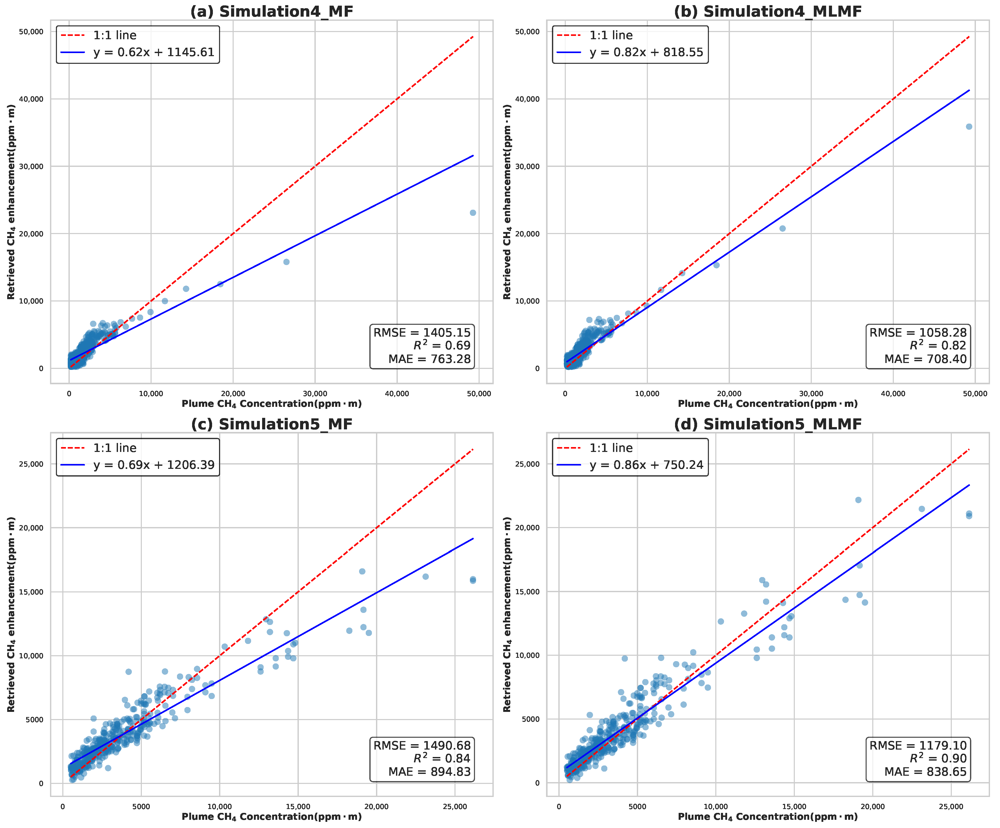
3.2. Algorithm Validation: Simulated Satellite Images with Overlaid Methane Plumes

To evaluate the performance of the MLMF at the image level, we constructed 100*100 pixel satellite images simulated with methane enhancement. This study employed five distinct simulated image construction processes. The first three simulations were based on radiance data simulated in Section 3.1. Simulation 1 applied random methane concentration enhancements to randomly selected pixels in the images. Simulations 2 and 3, on the other hand, introduced synthetic methane plumes modeled using a Gaussian distribution and a plume extracted from an EMIT methane plume product (Specifically, EMIT_L2B_CH4PLM_001_20240130T051816_002511), respectively.
To incorporate real-world variability and account for sensor noise, observation errors, and the effects of surface heterogeneity on retrievals, Simulations 4 and 5 utilized real satellite observations. Methane plume creation in these simulations followed the same methodology as Simulations 2 and 3. Using a 100*100 clipped segment of an actual AHSI observation, specifically the product GF5B_AHSI_E111.6_N35.8_20231031_011422_L10000412729_SW, served as the basis for the radiance data. Methane absorption was overlaid by modifying the original radiance spectrum using simulated absorption spectra derived from methane concentration enhancements. A summary of all simulations, the corresponding methane plume types, and image noise details is provided in Table 2 below.
The first part of the simulated image testing focused on random methane enhancement. In simulation 1, 2% of the pixels within the image were randomly selected and subjected to methane concentration enhancements. These enhancements were uniformly distributed within the range of 0–40,000 ppm·m. The absorption effects corresponding to these enhancements were embedded in the radiance spectra for the selected pixels. Retrieval experiments were then conducted using both the MF algorithm and the MLMF algorithm on this simulated radiance image with known methane concentrations.
From the results shown in Figure 4, the MLMF algorithm demonstrates superior retrieval performance across a wide range of methane concentration enhancements. The scatter plots clearly show that the MF results are consistent with prior spectral-level tests, exhibiting significant underestimation for high-concentration pixels and overestimation for moderate-concentration enhancements. Specifically, for high-concentration regions (e.g., pixels with enhancements around 40,000 ppm·m), the MF algorithm underestimates the retrieval by nearly 5000 ppm·m, corresponding to a relative error of approximately 10%. In contrast, for moderate-concentration regions (roughly 2500–25,000 ppm·m), the retrieved values are generally overestimated compared to the true values, resulting in noticeable deviations from the 1:1 reference line. These discrepancies indicate that the MF struggles to achieve consistent performance across different enhancement levels at the image scale.
In contrast, the MLMF exhibits a much more balanced and accurate performance. Across the entire enhancement range, the MLMF shows no significant overestimation or underestimation, and the retrieval errors do not increase with higher concentrations. This demonstrates that the MLMF maintains consistent performance across different concentration levels. From the linear regression results, the slope and intercept of the MLMF align more closely with the ideal 1:1 reference line. Additionally, the statistical metrics highlight the advantages of the MLMF: the RMSE decreases significantly from 1563.63 ppm·m (MF) to 337.09 ppm·m (MLMF), while the MAE drops from 1205.14 ppm·m to 442.88 ppm·m, indicating that the MLMF achieves far superior error control compared to the MF.
The second part of the simulated image testing involves pseudo-observational images overlaid with methane plumes. In this study, two distinct methane plumes were used to represent different spatial distributions of methane concentration. These include Plume 1, which is generated based on a 2D Gaussian diffusion model, and a detected methane emission plume from the EMIT plume product. To construct the test dataset, synthetic spectra were simulated, and methane absorption transmittance spectra were overlaid onto real satellite observations. Methane concentrations of the plume were scaled using different factor to achieve different emission rates, resulting in a total of 20 simulated images for the experiment. Figure 5 illustrates the 2300 nm radiance sample of the background region observed by the AHSI instrument, along with the spatial distribution of methane concentrations for the two plumes used for simulations.
Using both the MF and the MLMF, the entire image set was processed to retrieve the methane enhancement results. To compare methane concentration enhancement from the retrieval with the original simulated images, concentration thresholds were applied to obtain binary masks for methane plumes from both images. These masks were then multiplied to generate the final methane plume mask, where only the pixels present in both masks were included for algorithm comparison and further analysis.
Figure 6 presents a comparative analysis of the retrieval performance between the MF algorithm and the MLMF algorithm. The scatter plots illustrate the results obtained using simulated images generated from Simulation 2 (Gaussian plume) and Simulation 3 (EMIT plume product). Based on the results shown in the figure, it is evident that the MLMF outperforms the MF, particularly in high methane concentration enhancement regions.
Firstly, in terms of fitting results, the MLMF achieves linear regression slopes close to 1 and smaller intercepts under both simulation scenarios, indicating that the MLMF can more accurately capture methane concentration enhancements across different pixels. In contrast, the MF exhibits a noticeable underestimation trend as methane concentration enhancements increase. The MLMF demonstrates better linearity and consistency across concentration levels, effectively mitigating the underestimation issue of the MF in high-concentration regions.
From a statistical perspective, the MLMF shows significant improvements in multiple performance metrics:
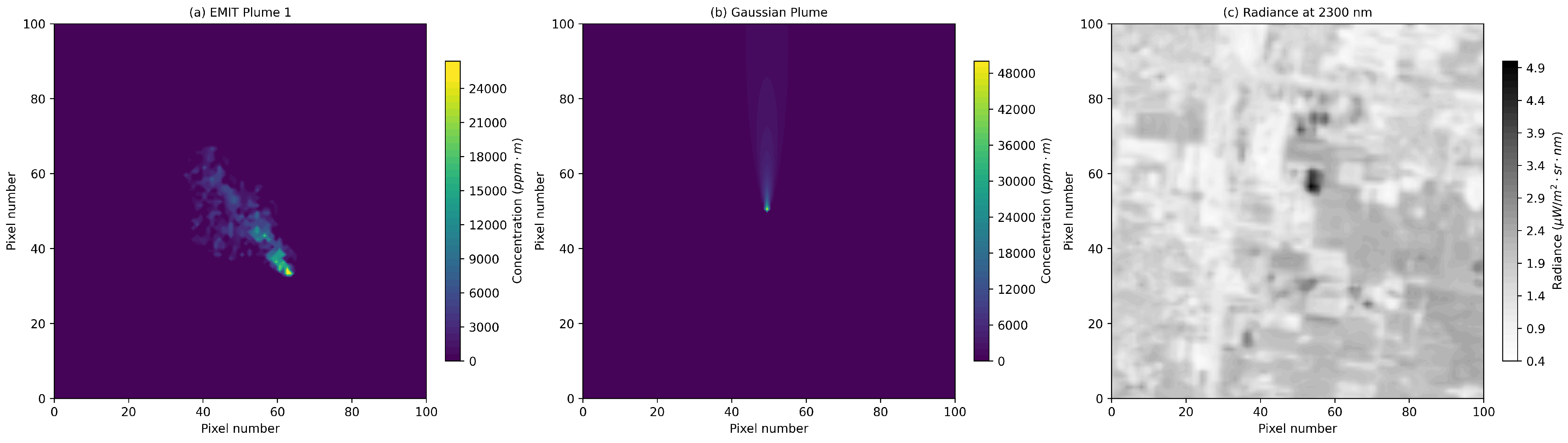
  • Gaussian plume simulation: The MLMF achieves a correlation coefficient ( R 2 ) of 0.98, a notable improvement compared to the MF ( R 2 = 0.91 ). Furthermore, the RMSE is reduced from 746 (ppm·m) in the MF to 345 in the MLMF, representing a 53.7% reduction. Similarly, the MAE decreases from 355.27 to 279.88, highlighting the higher accuracy of the MLMF.
  • EMIT plume product simulation: The MLMF achieves an even higher correlation coefficient of 0.99, demonstrating excellent fitting performance. The RMSE is reduced from 678 in the MF to 354 in the MLMF, a reduction of 47.8%. The MAE also decreases significantly, from 396.20 to 286.40, further validating the robustness of the MLMF in concentration enhancement retrieval.
Additionally, the plots reveal that the MLMF maintains a better alignment with the 1:1 line across medium-to-high concentration ranges, with scatter points more tightly clustered and exhibiting clearer trends. This indicates that the MLMF not only reduces retrieval errors but also achieves greater consistency and robustness across varying concentration levels.
Figure 7 presents the scatter plot comparison of the two algorithms for another two simulations, in which the same methane plumes were overlaid on the real AHSI observation sample. The figure highlights the comparative performance of the MF and the MLMF under conditions derived from real satellite observations overlaid with methane plumes. It is evident that the MLMF outperforms the MF in its ability to retrieve methane enhancements, particularly in high-concentration regions. As shown in the scatter plots, the MLMF achieves regression slopes closer to the ideal 1:1 line and smaller intercepts, indicating a better estimation of the methane plume concentration across a wide range of values. On the other hand, the MF consistently underestimates methane enhancements, especially at higher concentration levels, where the deviations from the 1:1 line are more pronounced. This highlights the MLMF’s ability to address the limitations of the MF in accurately capturing both low and high methane enhancements.
From the statistical metrics displayed in Figure 7, the MLMF provides significant improvements over the MF in both high- and moderate-concentration scenarios. For the high-concentration case (upper row), the MLMF reduces the RMSE from 1405.15 (MF) to 1058.28, a 24.7% reduction, and improves the correlation coefficient ( R 2 ) from 0.69 to 0.82. Similarly, the MAE decreases from 763.28 to 708.40. For the moderate-concentration case (lower row), the MLMF achieves an RMSE of 1179.10 compared to 1490.68 for the MF, a reduction of 20.9%, with the R 2 improving from 0.84 to 0.90. Additionally, the MLMF shows a more consistent fit to the 1:1 line, with tighter scatter distributions compared to the MF, reflecting better retrieval accuracy across different concentration levels.
Compared to the previous experiments based on simulated images, the retrieval accuracy in experiments with real satellite observations, as shown in Figure 7, is noticeably reduced. This decline is primarily due to the increased complexity and inherent uncertainties of real-world satellite data, which introduce challenges not present in the controlled simulations.
One key factor contributing to degradation is surface reflectance variability. Real satellite data are influenced by diverse land types (e.g., urban areas, forests, water bodies), causing discrepancies in radiance measurements and complicating background spectrum estimation and methane retrieval. Simulations 2 and 3, however, assume homogeneous surface reflectance, simplifying the retrieval process. Atmospheric effects, including water vapor, aerosols, and gases, further complicate methane retrieval by distorting the radiance spectrum, leading to inaccuracies in methane concentration estimates. Unlike simulated scenarios with ideal atmospheric conditions, real observations are affected by variable conditions, introducing additional uncertainty.
Sensor noise and calibration issues also introduce errors not typically accounted for in simulations. Satellite sensors experience imperfections and calibration drift, reducing retrieval accuracy, as reflected in the higher RMSE and MAE values in Simulations 4 and 5. These real-world uncertainties cause deviations from the ideal fit observed in simulations, complicating background spectrum estimation and covariance matrix calculation, which increases residuals and scatter plot spread. Nevertheless, despite these challenges, the multi-level matched filter consistently outperforms the traditional matched filter, demonstrating superior robustness and accuracy in handling heterogeneous radiative properties and enhancing background spectrum estimation.
In conclusion, while real-world satellite observations pose significant challenges, the MLMF method offers a notable improvement over traditional methods. Its effectiveness under these conditions underscores its potential for reliable methane detection and quantification in practical applications.

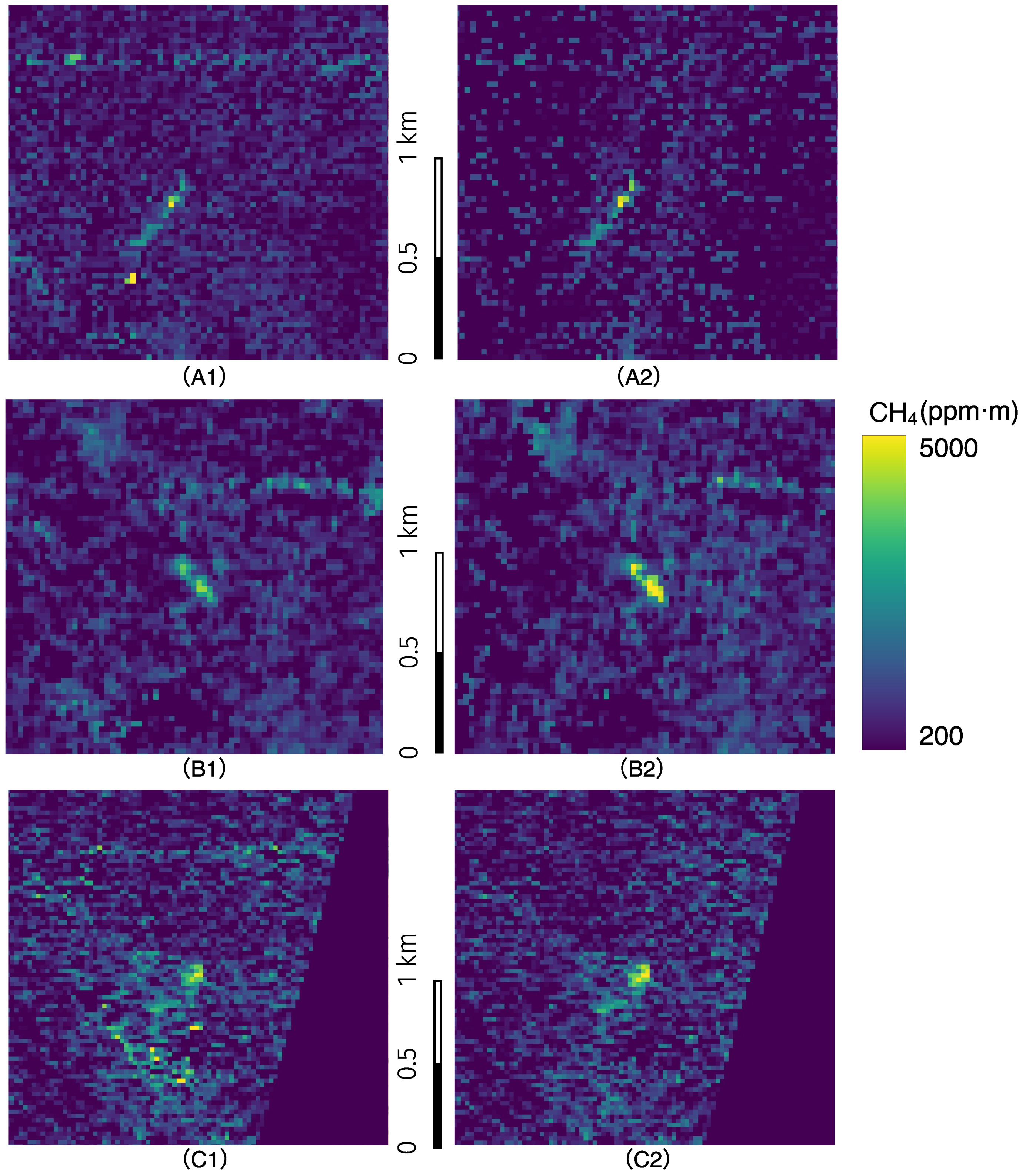
3.3. Algorithm Validation: Controlled Release Experiment

The MLMF algorithm was further validated using spaceborne hyper-spectral images obtained during the Stanford controlled release experiment, given the ground-based measurements of methane and wind data. Based on the Δ X C H 4 mapping results from both the MF and the MLMF, methane plumes were successfully captured in all three scenes of images, as shown in Figure 8.
When comparing the inversion results of the two algorithms, the MLMF outperforms the MF in several key aspects. First, the contrast between the plume and the background is much higher in the MLMF, making the plume more distinct. Additionally, the concentration values within the plume are higher, indicating a more accurate inversion of methane concentration. This improvement is partly due to the fact that the MLMF applies more appropriate unit absorption spectra to background pixels, which leads to a significant reduction in background noise. Moreover, some artifacts, such as mountains and roads, which were present in the MF results, are minimized in the MLMF output. These improvements collectively contribute to more precise methane plume detection and reduce the risk of missing plumes during monitoring.
After the methane plume extraction process, the methane emission flux rates were estimated using the IME model, with the ground-based methane and wind data serving as the reference. The scatter plots and key statistics presented in Figure 9 highlight the superior performance of the MLMF algorithm over the MF approach in estimating methane emission flux rates. The MLMF achieves a regression slope of 0.96, closer to the ideal value of 1, and a higher correlation coefficient (R² = 0.9589) compared to the MF (R² = 0.7077). Furthermore, it substantially reduces estimation errors, with RMSE decreasing by 82.55% (from 92.32 kg/h to 16.10 kg/h) and MAE decreasing by 81.79% (from 76.97 kg/h to 14.02 kg/h). These improvements highlight the ability of the MLMF to address the underestimation bias present in the MF, leading to more accurate and reliable quantification of methane emission flux rates. The reduced error bars and consistent performance across multiple datasets further reinforce the robustness of the MLMF algorithm.
Although the controlled release experiment took place in a desert with relatively homogeneous surface conditions and favorable weather, real-world conditions often introduce additional complexities that affect methane emission estimations. One such factor is cloud cover, which can obstruct satellite observations, leading to scattering and absorption of the signal. This reduces the signal-to-noise ratio and introduces uncertainties in methane concentration retrievals. Furthermore, surface heterogeneity—such as varying land types, urban areas, or forests—can cause discrepancies in radiance measurements, affecting the accuracy of methane plume detection and background spectra estimation. In real-world environments, these variations are more pronounced compared to the relatively uniform desert terrain used in the experiment. Additionally, the wind speed data used for estimating methane emission fluxes are typically derived from coarse reanalysis datasets, which may not fully capture local wind patterns or turbulent conditions, especially in regions with complex topography. These inaccuracies in wind speed measurements can lead to errors in emission rate estimation. Given these factors, methane emission estimations in real-world scenarios are subject to greater variability, and while the MLMF algorithm performs well under controlled conditions, additional uncertainties should be accounted for when applying it to more complex, real-world environments.

4. Discussion

This study proposes a multi-level matched filter algorithm based on hierarchical cumulative computation to optimize methane column concentration enhancement retrieval and emission rate estimation. The MLMF algorithm incorporates a radiance LUT to generate appropriate unit absorption spectra in real-time, tailored for different scenarios and concentration retrieval intervals. The algorithm divides pixels in the image into background and potential methane emission pixels, processing them differently to optimize the results. Specifically, background pixels are processed using a more accurate unit absorption spectrum fitted within a smaller range, which reduces the standard deviation of background inversion results, mitigates noise interference, and minimizes the mixing of background and plume pixels. For methane emission pixels, different background spectra are constructed to accumulate concentration enhancements based on relative threshold values for each interval. This method effectively addresses issues of background interference and the underestimation of high emissions typically observed in traditional MF algorithms, thereby improving the accuracy of methane emission leakage monitoring and emission quantification.
In this study, the MLMF algorithm was validated in three stages:
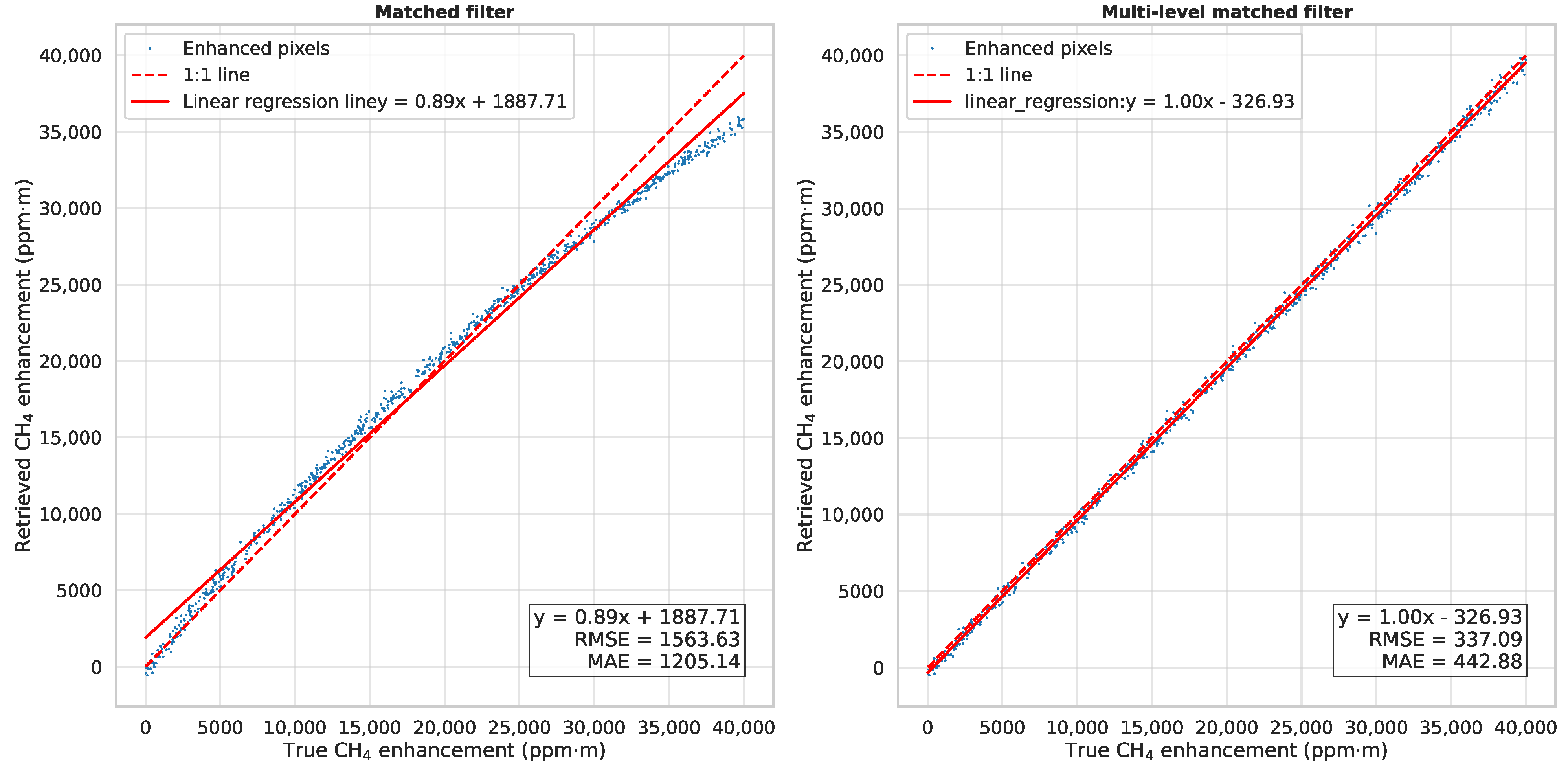
  • Spectral Residual Fitting: The first stage involved spectral residual fitting without considering noise or sensor spectral resolution to evaluate the MLMF’s performance. The results demonstrate that the MLMF significantly mitigates the underestimation issue for high methane concentration enhancements that arise from the linear assumptions of traditional MF algorithms. Relative errors were reduced from up to −30% to within ±5% at high concentrations, and the regression slope improved from 0.89 to 1.00, indicating the MLMF’s ability to better approximate the nonlinear relationship between methane concentration and absorption.
  • Simulated Data Tests: The second stage tested the algorithm using simulated data, including randomly enhanced methane concentration pixels, synthetic Gaussian methane plumes, and EMIT plume products. The MLMF achieved better retrieval accuracy across a wide range of concentration enhancements (0–40,000 ppm·m), with RMSE reduced from 1563.63 ppm·m to 337.09 ppm·m and MAE decreased from 1205.14 ppm·m to 442.88 ppm·m compared to the MF. In plume-based simulations, the MLMF outperformed the MF, particularly in high-concentration regions, improving R 2 from 0.91 to 0.98 for Gaussian plumes and achieving an R 2 of 0.99 for EMIT plume simulations, with RMSE reductions of 53.7
  • Controlled Release Experiment: The third stage involved validating the MLMF using satellite data from controlled release experiments along with ground-truth emission rate measurements. The results indicated that the MLMF provided a higher contrast between the plume and the background, resulting in more accurate methane concentration retrievals and fewer artifacts compared to the MF. These improvements led to better plume quantification and enhanced the reliability of methane emission estimates, with emission rate accuracy improving significantly. The R² value increased from 0.71 to 0.96, and RMSE reduced from 92.32 kg/h to 16.10 kg/h.
Despite the significant improvements brought by the MLMF algorithm, particularly in addressing the underestimation of high-concentration methane plumes, some challenges remain. One of the main limitations is the current radiance LUT, which does not fully incorporate factors such as view zenith angle and water vapor content, both of which can impact methane retrieval accuracy, and sensor altitudes lower than 100km, bringing MLMF into airborne instrumental methane mapping. Another challenge lies in the calculation of the unit absorption spectra before algorithm execution, which introduces computational overhead. While using a pre-calculated unit absorption spectrum LUT instead of a radiance LUT can speed up the algorithm, the time-consuming process of constructing the table remains a bottleneck. Future iterations could benefit from more powerful computational resources to optimize the LUT construction process, improving efficiency, especially for large datasets and real-time applications.
Looking forward, improvements to the MLMF algorithm could focus on two key internal optimizations. First, the fixed segmentation approach for methane concentration retrieval intervals could be enhanced by implementing a dynamic segmentation method. This would allow the algorithm to adjust to emissions of different scales, improving scalability and flexibility for varying scenarios. Second, conducting a methane sensitivity analysis could help identify the most relevant spectral bands for methane retrieval. By selectively using these bands, the algorithm could reduce interference from confounding factors like water vapor and carbon monoxide, while also decreasing the amount of spectral data processed. These changes would improve both the efficiency and accuracy of the MLMF in real-world applications.
While the MLMF significantly improves methane emission quantification, its computational complexity—arising from pixel segmentation, multiple iterations, and reliance on the radiance LUT—presents challenges for large-scale applications. The need to perform iterative corrections and use the LUT for absorption spectrum matching can lead to substantial processing time, which becomes a bottleneck when handling large datasets or real-time satellite data. To overcome these challenges, parallel processing and algorithm optimization (such as leveraging GPU acceleration or distributed computing) could improve the efficiency of the MLMF, enabling it to process larger datasets more effectively. Additionally, reducing the number of iterations required for concentration estimation and optimizing the LUT construction process by streamlining pre-calculation and reducing unnecessary complexity would help speed up the overall algorithm. These improvements would enhance the MLMF’s capability for real-time data processing, making it more suitable for operational monitoring tasks that require fast turnaround times and the ability to handle large-scale data efficiently.
Lastly, we would like to highlight that the MLMF algorithm can be integrated with other advancements in methane retrieval, such as albedo correction, sparsity assumption, and retrieval window combination. These approaches, commonly used in previous studies, do not conflict with the MLMF method and could be combined to achieve even better performance. However, the exact implementation and benefits of combining these techniques with MLMF require further research and experimentation.

5. Conclusions

In this study, we proposed the multi-level matched filter (MLMF) algorithm, which significantly improves the accuracy of methane concentration retrieval and emission rate estimation. The MLMF mitigates the underestimation issue commonly found in traditional matched filter algorithms, particularly at high methane concentrations, by incorporating piecewise regression and using a radiance look-up table for more accurate plume detection and quantification. Validation results show that the MLMF outperforms traditional MF algorithms across simulated and real-world data, with RMSE reductions, increased R 2 values, and improved emission rate estimates.
The MLMF algorithm’s ability to enhance methane detection across various concentration ranges and sensor types has important implications for satellite-based methane monitoring. It provides more reliable quantification of methane emissions and better identification of methane hotspots, which is crucial for effective climate change mitigation efforts. The algorithm can be used to support emission inventories and inform regional policy development for methane reduction. While the MLMF algorithm offers substantial improvements over existing methods, further optimization is necessary to address computational limitations and enhance its applicability to a broader range of scenarios. Future improvements include dynamic segmentation for methane concentration intervals and methane sensitivity analysis to select optimal retrieval bands, which would improve efficiency and reduce interference from other atmospheric factors.
The MLMF algorithm represents a significant advancement in methane detection and monitoring, enhancing both the accuracy and reliability of methane emission quantification from satellite data. By addressing key challenges and incorporating suggestions for future improvements, the MLMF algorithm will continue to be a valuable tool for climate change mitigation, particularly in identifying and quantifying methane hotspots and improving emission monitoring practices.

Author Contributions

Conceptualization M.L., Y.Z. and L.C.; data collection and experiment conduction, M.L. and Y.Z.; funding acquisition, Y.Z., L.C. and J.T.; research supervision, Y.Z. and L.C.; original draft, M.L.; review and editing, Y.Z., J.T., M.F. and C.Y. All authors have read and agreed to the published version of the manuscript.

Funding

This research was supported by the National Key Research and Development Program of China (Grant No. 2022YFB3904800), the National Natural Science Foundation of China (Grant No. 42171393), and the Tianfu Yongxing Laboratory Organized Research Project (Grant No. 2024KJGG18).

Data Availability Statement

Data will be made available upon request.

Acknowledgments

We sincerely acknowledge the availability of the public plume dataset provided by EMIT and the open data shared by EnMAP. We are also grateful to the contributors of the controlled-release experiments for supplying emission data and ground-based meteorological data. What is more, we would like to thank Zhongting Wang, Chunyan Zhou, and Wei Zhou from the Satellite Application Center for Ecology and Environment, Ministry of Ecology and Environment of the People’s Republic of China, as well as Fei Li from Nanjing University, for their invaluable assistance in providing several pieces of satellite data used in this study. Finally, we would like to express our gratitude to the open-source Python libraries, such as Matplotlib and Seaborn, which greatly facilitated the processing and visualization of our data and results.

Conflicts of Interest

The authors declare no conflicts of interest.

Abbreviations

The following abbreviations are used in this manuscript:
AHSIAdvanced HyperSpectral Imager
FWHMFull Width at Half Maximum
IMEIntegrated Mass Enhancement
LUTLook-Up Table
MFMatched Filter
MLMFMulti-Level Matched Filter
MAEMean Absolute Error
RMSERoot Mean Squared Error
SNRSignal-to-Noise Ratio
SWIRShortWave InfraRed
SZASolar Zenith Angle

References

  1. Xie, G.Z.; Zhang, L.P.; Li, C.Y.; Sun, W.D. Accelerated Methane Emission from Permafrost Regions since the 20th Century. Deep. Sea Res. Part I Oceanogr. Res. Pap. 2023, 195, 103981. [Google Scholar] [CrossRef]
  2. Shen, L.; Jacob, D.J.; Gautam, R.; Omara, M.; Scarpelli, T.R.; Lorente, A.; Zavala-Araiza, D.; Lu, X.; Chen, Z.; Lin, J. National Quantifications of Methane Emissions from Fuel Exploitation Using High Resolution Inversions of Satellite Observations. Nat. Commun. 2023, 14, 4948. [Google Scholar] [CrossRef] [PubMed]
  3. Zhang, Y.; Jacob, D.J.; Lu, X.; Maasakkers, J.D.; Scarpelli, T.R.; Sheng, J.X.; Shen, L.; Qu, Z.; Sulprizio, M.P.; Chang, J.; et al. Attribution of the Accelerating Increase in Atmospheric Methane during 2010–2018 by Inverse Analysis of GOSAT Observations. Atmos. Chem. Phys. 2021, 21, 3643–3666. [Google Scholar] [CrossRef]
  4. Prather, M.J.; Holmes, C.D.; Hsu, J. Reactive Greenhouse Gas Scenarios: Systematic Exploration of Uncertainties and the Role of Atmospheric Chemistry. Geophys. Res. Lett. 2012, 39, 2012GL051440. [Google Scholar] [CrossRef]
  5. Nisbet, E.G.; Manning, M.R.; Dlugokencky, E.J.; Michel, S.E.; Lan, X.; Röckmann, T.; Denier Van Der Gon, H.A.C.; Schmitt, J.; Palmer, P.I.; Dyonisius, M.N.; et al. Atmospheric Methane: Comparison Between Methane’s Record in 2006–2022 and During Glacial Terminations. Glob. Biogeochem. Cycles 2023, 37, e2023GB007875. [Google Scholar] [CrossRef]
  6. Nisbet, E.G.; Fisher, R.E.; Lowry, D.; France, J.L.; Allen, G.; Bakkaloglu, S.; Broderick, T.J.; Cain, M.; Coleman, M.; Fernandez, J.; et al. Methane Mitigation: Methods to Reduce Emissions, on the Path to the Paris Agreement. Rev. Geophys. 2020, 58, e2019RG000675. [Google Scholar] [CrossRef]
  7. Isaksen, I.; Berntsen, T.; Dalsøren, S.; Eleftheratos, K.; Orsolini, Y.; Rognerud, B.; Stordal, F.; Søvde, O.; Zerefos, C.; Holmes, C. Atmospheric Ozone and Methane in a Changing Climate. Atmosphere 2014, 5, 518–535. [Google Scholar] [CrossRef]
  8. Kirschke, S.; Bousquet, P.; Ciais, P.; Saunois, M.; Canadell, J.G.; Dlugokencky, E.J.; Bergamaschi, P.; Bergmann, D.; Blake, D.R.; Bruhwiler, L.; et al. Three Decades of Global Methane Sources and Sinks. Nat. Geosci. 2013, 6, 813–823. [Google Scholar] [CrossRef]
  9. Brandt, A.R.; Heath, G.A.; Kort, E.A.; O’Sullivan, F.; Petron, G.; Jordaan, S.M.; Tans, P.; Wilcox, J.; Gopstein, A.M.; Arent, D.; et al. Methane Leaks from North American Natural Gas Systems. Science 2014, 343, 733–735. [Google Scholar] [CrossRef]
  10. Brandt, A.R.; Heath, G.A.; Cooley, D. Methane Leaks from Natural Gas Systems Follow Extreme Distributions. Environ. Sci. Technol. 2016, 50, 12512–12520. [Google Scholar] [CrossRef]
  11. Frankenberg, C.; Thorpe, A.K.; Thompson, D.R.; Hulley, G.; Kort, E.A.; Vance, N.; Borchardt, J.; Krings, T.; Gerilowski, K.; Sweeney, C.; et al. Airborne Methane Remote Measurements Reveal Heavy-Tail Flux Distribution in Four Corners Region. Proc. Natl. Acad. Sci. USA 2016, 113, 9734–9739. [Google Scholar] [CrossRef] [PubMed]
  12. Barré, J.; Aben, I.; Agustí-Panareda, A.; Balsamo, G.; Bousserez, N.; Dueben, P.; Engelen, R.; Inness, A.; Lorente, A.; McNorton, J.; et al. Systematic Detection of Local CH4 Anomalies by Combining Satellite Measurements with High-Resolution Forecasts. Atmos. Chem. Phys. 2021, 21, 5117–5136. [Google Scholar] [CrossRef]
  13. Varon, D.J.; Jervis, D.; McKeever, J.; Spence, I.; Gains, D.; Jacob, D.J. High-Frequency Monitoring of Anomalous Methane Point Sources with Multispectral Sentinel-2 Satellite Observations. Atmos. Meas. Tech. Discuss. 2020, 14, 2771–2785. [Google Scholar] [CrossRef]
  14. Jacob, D.J.; Turner, A.J.; Maasakkers, J.D.; Sheng, J.; Sun, K.; Liu, X.; Chance, K.; Aben, I.; McKeever, J.; Frankenberg, C. Satellite Observations of Atmospheric Methane and Their Value for Quantifying Methane Emissions. Atmos. Chem. Phys. 2016, 16, 14371–14396. [Google Scholar] [CrossRef]
  15. Duren, R.M.; Thorpe, A.K.; Foster, K.T.; Rafiq, T.; Hopkins, F.M.; Yadav, V.; Bue, B.D.; Thompson, D.R.; Conley, S.; Colombi, N.K.; et al. California’s Methane Super-Emitters. Nature 2019, 575, 180–184. [Google Scholar] [CrossRef]
  16. Jervis, D.; McKeever, J.; Durak, B.O.A.; Sloan, J.J.; Gains, D.; Varon, D.J.; Ramier, A.; Strupler, M.; Tarrant, E. The GHGSat-D Imaging Spectrometer. Atmos. Meas. Tech. 2021, 14, 2127–2140. [Google Scholar] [CrossRef]
  17. Cusworth, D.H.; Duren, R.M.; Thorpe, A.K.; Pandey, S.; Maasakkers, J.D.; Aben, I.; Jervis, D.; Varon, D.J.; Jacob, D.J.; Randles, C.A.; et al. Multisatellite Imaging of a Gas Well Blowout Enables Quantification of Total Methane Emissions. Geophys. Res. Lett. 2021, 48, e2020GL090864. [Google Scholar] [CrossRef]
  18. Lyon, D.R.; Hmiel, B.; Gautam, R.; Omara, M.; Roberts, K.A.; Barkley, Z.R.; Davis, K.J.; Miles, N.L.; Monteiro, V.C.; Richardson, S.J.; et al. Concurrent Variation in Oil and Gas Methane Emissions and Oil Price during the COVID-19 Pandemic. Atmos. Chem. Phys. 2021, 21, 6605–6626. [Google Scholar] [CrossRef]
  19. Zhang, Y.; Gautam, R.; Pandey, S.; Omara, M.; Maasakkers, J.D.; Sadavarte, P.; Lyon, D.; Nesser, H.; Sulprizio, M.P.; Varon, D.J.; et al. Quantifying Methane Emissions from the Largest Oil-Producing Basin in the United States from Space. Sci. Adv. 2020, 6, eaaz5120. [Google Scholar] [CrossRef]
  20. Varon, D.J.; Jacob, D.J.; Jervis, D.; McKeever, J. Quantifying Time-Averaged Methane Emissions from Individual Coal Mine Vents with GHGSat-D Satellite Observations. Environ. Sci. Technol. 2020, 54, 10246–10253. [Google Scholar] [CrossRef]
  21. Marjani, M.; Mohammadimanesh, F.; Varon, D.J.; Radman, A.; Mahdianpari, M. PRISMethaNet: A Novel Deep Learning Model for Landfill Methane Detection Using PRISMA Satellite Data. ISPRS J. Photogramm. Remote Sens. 2024, 218, 802–818. [Google Scholar] [CrossRef]
  22. Frankenberg, C.; Platt, U.; Wagner, T. Iterative Maximum a Posteriori (IMAP)-DOAS for Retrieval of Strongly Absorbing Trace Gases: Model Studies for CH4 and CO2 Retrieval from near Infrared Spectra of SCIAMACHY Onboard. Atmos. Chem. Phys. 2005, 5, 9–12. [Google Scholar] [CrossRef]
  23. Lorente, A.; Borsdorff, T.; Butz, A.; Hasekamp, O.; Aan De Brugh, J.; Schneider, A.; Wu, L.; Hase, F.; Kivi, R.; Wunch, D.; et al. Methane Retrieved from TROPOMI: Improvement of the Data Product and Validation of the First 2 Years of Measurements. Atmos. Meas. Tech. 2021, 14, 665–684. [Google Scholar] [CrossRef]
  24. Thorpe, A.K.; Frankenberg, C.; Thompson, D.R.; Duren, R.M.; Aubrey, A.D.; Bue, B.D.; Green, R.O.; Gerilowski, K.; Krings, T.; Borchardt, J.; et al. Airborne DOAS Retrievals of Methane, Carbon Dioxide, and Water Vapor Concentrations at High Spatial Resolution: Application to AVIRIS-NG. Atmos. Meas. Tech. 2017, 10, 3833–3850. [Google Scholar] [CrossRef]
  25. Thompson, D.R.; Leifer, I.; Bovensmann, H.; Eastwood, M.; Fladeland, M.; Frankenberg, C.; Gerilowski, K.; Green, R.O.; Kratwurst, S.; Krings, T.; et al. Real-Time Remote Detection and Measurement for Airborne Imaging Spectroscopy: A Case Study with Methane. Atmos. Meas. Tech. 2015, 8, 4383–4397. [Google Scholar] [CrossRef]
  26. Foote, M.D.; Dennison, P.E.; Thorpe, A.K.; Thompson, D.R.; Jongaramrungruang, S.; Frankenberg, C.; Joshi, S.C. Fast and Accurate Retrieval of Methane Concentration from Imaging Spectrometer Data Using Sparsity Prior. IEEE Trans. Geosci. Remote Sens. 2020, 58, 6480–6492. [Google Scholar] [CrossRef]
  27. Cusworth, D.H.; Duren, R.M.; Thorpe, A.K.; Olson-Duvall, W.; Heckler, J.; Chapman, J.W.; Eastwood, M.L.; Helmlinger, M.C.; Green, R.O.; Asner, G.P.; et al. Intermittency of Large Methane Emitters in the Permian Basin. Environ. Sci. Technol. Lett. 2021, 8, 567–573. [Google Scholar] [CrossRef]
  28. Thompson, D.R.; Thorpe, A.K.; Frankenberg, C.; Green, R.O.; Duren, R.; Guanter, L.; Hollstein, A.; Middleton, E.; Ong, L.; Ungar, S. Space-based Remote Imaging Spectroscopy of the Aliso Canyon CH4 Superemitter. Geophys. Res. Lett. 2016, 43, 6571–6578. [Google Scholar] [CrossRef]
  29. Guanter, L.; Irakulis-Loitxate, I.; Gorroño, J.; Sánchez-García, E.; Cusworth, D.H.; Varon, D.J.; Cogliati, S.; Colombo, R. Mapping Methane Point Emissions with the PRISMA Spaceborne Imaging Spectrometer. Remote Sens. Environ. 2021, 265, 112671. [Google Scholar] [CrossRef]
  30. Irakulis-Loitxate, I.; Guanter, L.; Liu, Y.N.; Varon, D.J.; Maasakkers, J.D.; Zhang, Y.; Chulakadabba, A.; Wofsy, S.C.; Thorpe, A.K.; Duren, R.M.; et al. Satellite-Based Survey of Extreme Methane Emissions in the Permian Basin. Sci. Adv. 2021, 7, eabf4507. [Google Scholar] [CrossRef]
  31. Schaum, A. A Uniformly Most Powerful Detector of Gas Plumes against a Cluttered Background. Remote Sens. Environ. 2021, 260, 112443. [Google Scholar] [CrossRef]
  32. Pei, Z.; Han, G.; Mao, H.; Chen, C.; Shi, T.; Yang, K.; Ma, X.; Gong, W. Improving Quantification of Methane Point Source Emissions from Imaging Spectroscopy. Remote Sens. Environ. 2023, 295, 113652. [Google Scholar] [CrossRef]
  33. Roger, J.; Guanter, L.; Gorroño, J.; Irakulis-Loitxate, I. Exploiting the Entire Near-Infrared Spectral Range to Improve the Detection of Methane Plumes with High-Resolution Imaging Spectrometers. Atmos. Meas. Tech. Discuss. 2023, 17, 1333–1346. [Google Scholar] [CrossRef]
  34. Sherwin, E.D.; El Abbadi, S.H.; Burdeau, P.M.; Zhang, Z.; Chen, Z.; Rutherford, J.S.; Chen, Y.; Brandt, A.R. Single-Blind Test of Nine Methane-Sensing Satellite Systems from Three Continents. Atmos. Meas. Tech. 2024, 17, 765–782. [Google Scholar] [CrossRef]
  35. Sánchez-García, E.; Gorroño, J.; Irakulis-Loitxate, I.; Varon, D.J.; Guanter, L. Mapping Methane Plumes at Very High Spatial Resolution with the WorldView-3 Satellite. Atmos. Meas. Tech. 2022, 15, 1657–1674. [Google Scholar] [CrossRef]
  36. Ayasse, A.K.; Dennison, P.E.; Foote, M.; Thorpe, A.K.; Joshi, S.; Green, R.O.; Duren, R.M.; Thompson, D.R.; Roberts, D.A. Methane Mapping with Future Satellite Imaging Spectrometers. Remote Sens. 2019, 11, 3054. [Google Scholar] [CrossRef]
  37. Li, F.; Sun, S.; Zhang, Y.; Feng, C.; Chen, C.; Mao, H.; Liu, Y. Mapping Methane Super-Emitters in China and United States with GF5-02 Hyperspectral Imaging Spectrometer. Natl. Remote Sens. Bull. 2023, 28, 986–2001. [Google Scholar] [CrossRef]
  38. Liu, Y.N.; Zhang, J.; Zhang, Y.; Sun, W.W.; Jiao, L.L.; Sun, D.X.; Hu, X.N.; Ye, X.; Li, Y.D.; Liu, S.F.; et al. The Advanced Hyperspectral Imager: Aboard China’s GaoFen-5 Satellite. IEEE Geosci. Remote Sens. Mag. 2019, 7, 23–32. [Google Scholar] [CrossRef]
  39. He, Z.; Gao, L.; Liang, M.; Zeng, Z.C. A Survey of Methane Point Source Emissions from Coal Mines in Shanxi Province of China Using AHSI on Board Gaofen-5B. Atmos. Meas. Tech. 2024, 17, 2937–2956. [Google Scholar] [CrossRef]
  40. Roger, J.; Irakulis-Loitxate, I.; Valverde, A.; Gorroño, J.; Chabrillat, S.; Brell, M.; Guanter, L. High-Resolution Methane Mapping with the EnMAP Satellite Imaging Spectroscopy Mission. IEEE Trans. Geosci. Remote Sens. 2024, 62, 1–12. [Google Scholar] [CrossRef]
  41. Foote, M.D.; Dennison, P.E.; Sullivan, P.R.; O’Neill, K.B.; Thorpe, A.K.; Thompson, D.R.; Cusworth, D.H.; Duren, R.; Joshi, S.C. Impact of Scene-Specific Enhancement Spectra on Matched Filter Greenhouse Gas Retrievals from Imaging Spectroscopy. Remote Sens. Environ. 2021, 264, 112574. [Google Scholar] [CrossRef]
  42. Manolakis, D.; Truslow, E.; Pieper, M.; Cooley, T.; Brueggeman, M. Detection Algorithms in Hyperspectral Imaging Systems: An Overview of Practical Algorithms. IEEE Signal Process. Mag. 2013, 31, 24–33. [Google Scholar] [CrossRef]
  43. Funk, C.; Theiler, J.; Roberts, D.; Borel, C. Clustering to Improve Matched Filter Detection of Weak Gas Plumes in Hyperspectral Thermal Imagery. IEEE Trans. Geosci. Remote Sens. 2001, 39, 1410–1420. [Google Scholar] [CrossRef]
  44. Allen, D. Attributing Atmospheric Methane to Anthropogenic Emission Sources. Accounts Chem. Res. 2016, 49, 1344–1350. [Google Scholar] [CrossRef]
  45. Thorpe, A.K.; Roberts, D.A.; Bradley, E.S.; Funk, C.C.; Dennison, P.E.; Leifer, I. High Resolution Mapping of Methane Emissions from Marine and Terrestrial Sources Using a Cluster-Tuned Matched Filter Technique and Imaging Spectrometry. Remote Sens. Environ. 2013, 134, 305–318. [Google Scholar] [CrossRef]
  46. Berk, A.; Conforti, P.; Kennett, R.; Perkins, T.; Hawes, F.; Van Den Bosch, J. MODTRAN® 6: A Major Upgrade of the MODTRAN® Radiative Transfer Code. In Proceedings of the 2014 6th Workshop on Hyperspectral Image and Signal Processing: Evolution in Remote Sensing (WHISPERS), Lausanne, Switzerland, 24–27 June 2014; pp. 1–4. [Google Scholar] [CrossRef]
  47. Yang, S.; Yang, J.; Shi, S.; Song, S.; Luo, Y.; Du, L. The Rising Impact of Urbanization-Caused CO2 Emissions on Terrestrial Vegetation. Ecol. Indic. 2023, 148, 110079. [Google Scholar] [CrossRef]
  48. Guanter, L.; Richter, R.; Moreno, J. Spectral Calibration of Hyperspectral Imagery Using Atmospheric Absorption Features. Appl. Opt. 2006, 45, 2360. [Google Scholar] [CrossRef]
  49. Lyon, D.R.; Alvarez, R.A.; Zavala-Araiza, D.; Brandt, A.R.; Jackson, R.B.; Hamburg, S.P. Aerial Surveys of Elevated Hydrocarbon Emissions from Oil and Gas Production Sites. Environ. Sci. Technol. 2016, 50, 4877–4886. [Google Scholar] [CrossRef]
  50. Shi, T.; Han, G.; Ma, X.; Mao, H.; Chen, C.; Han, Z.; Pei, Z.; Zhang, H.; Li, S.; Gong, W. Quantifying Factory-Scale CO2 /CH4 Emission Based on Mobile Measurements and EMISSION-PARTITION Model: Cases in China. Environ. Res. Lett. 2023, 18, 034028. [Google Scholar] [CrossRef]
  51. Conley, S.; Franco, G.; Faloona, I.; Blake, D.R.; Peischl, J.; Ryerson, T.B. Methane Emissions from the 2015 Aliso Canyon Blowout in Los Angeles, CA. Science 2016, 351, 1317–1320. [Google Scholar] [CrossRef]
  52. Varon, D.J.; Jacob, D.J.; McKeever, J.; Jervis, D.; Durak, B.O.A.; Xia, Y.; Huang, Y. Quantifying Methane Point Sources from Fine-Scale Satellite Observations of Atmospheric Methane Plumes. Atmos. Meas. Tech. 2018, 11, 5673–5686. [Google Scholar] [CrossRef]
  53. Zheng, B.; Chevallier, F.; Ciais, P.; Broquet, G.; Wang, Y.; Lian, J.; Zhao, Y. Observing Carbon Dioxide Emissions over China’s Cities and Industrial Areas with the Orbiting Carbon Observatory-2. Atmos. Chem. Phys. 2020, 20, 8501–8510. [Google Scholar] [CrossRef]
  54. Cusworth, D.H.; Duren, R.M.; Thorpe, A.K.; Tseng, E.; Thompson, D.; Guha, A.; Newman, S.; Foster, K.T.; Miller, C.E. Using Remote Sensing to Detect, Validate, and Quantify Methane Emissions from California Solid Waste Operations. Atmos. Chem. Phys. 2020, 15, 054012. [Google Scholar] [CrossRef]
Figure 1. Spatial coverage of the data from three selected satellites of the controlled release experiment: EnMAP observation is represented by a green rectangle, GF5B observation is represented by a brown rectangle, and ZY1F observation is represented by a blue rectangle. The location of release stacks is pinpointed as a star. The background true-color image of the study area is from Google Earth WMS.
Remotesensing 17 00843 g001
Figure 2. The unit absorption spectra under different radiative transfer simulation parameters: (a) different surface altitudes, (b) different solar zenith angles (SZA), (c) varying methane concentration enhancement ranges with fixed background value, and (d) different initial methane concentration enhancement values with a constant range of 10,000 ppm·m.
Remotesensing 17 00843 g002
Figure 3. Comparison of two matched filter algorithms: the MF with different unit absorption spectra and MLMF. (a) Relative bias (%) of retrievals across various CH4 enhancements. (b) Absolute bias (ppm·m) of retrievals. (c) Linear regression for retrievals from each testing set, with the black dashed line representing the 1:1 reference line. In all subplots, the red line represents MLMF results, while other colored lines show MF performance using different unit absorption spectra ranging from 10,000 to 50,000 ppm·m.
Remotesensing 17 00843 g003
Figure 4. Comparison of retrieval performance between the MF (left) and the MLMF (right). The scatter plots show the retrieved methane concentration enhancement values versus the true simulated enhancements, ranging from 0 to 40,000 ppm·m. The blue scatter points represent the enhanced pixels, the red lines are the linear regressions of the retrievals against the true enhancements, and the red dashed line indicates the 1:1 reference. The MLMF algorithm demonstrates superior accuracy, with the scatter points aligning more closely to the 1:1 line and the regression slope approaching the ideal value of 1, compared to the MF algorithm.
Remotesensing 17 00843 g004
Figure 5. A 100*100 clip of the plumes used in image simulation and background radiance. (a) Methane plume sample from the EMIT plume product dataset. (b) Synthetic plume that follows a Gaussian distribution as input for end-to-end simulation. (c) Radiance at 2300 nm from the GF5B AHSI instrument from an emission-free observation on 31 October 2023.
Remotesensing 17 00843 g005
Figure 6. Comparison of methane plume retrieval performance between the MF and the MLMF algorithms using simulated images based on radiative transfer simulation. The scatter plots show the relationship between the retrieved methane enhancement and true plume methane concentration (both in ppm·m). (a,b) show the results from Simulation 2 using Gaussian-distributed plumes for the MF and MLMF algorithms, respectively. (c,d) present the results from Simulation 3 based on EMIT plume products for the MF and MLMF algorithms, respectively. In each panel, the red dashed line represents the 1:1 reference line, while the blue solid line shows the linear fit to the data. Statistical metrics, including RMSE, R 2 , and MAE, are provided in the bottom right corner of each panel.
Remotesensing 17 00843 g006
Figure 7. Comparison of methane plume retrieval performance between the MF and the MLMF algorithms using simulated images based on real satellite observation. The scatter plots show the relationship between the retrieved methane enhancement and true plume methane concentration (both in ppm·m). (a,b) show the results from Simulation 4 for the MF and MLMF algorithms, respectively. (c,d) present the results from Simulations 5 for the MF and MLMF algorithms, respectively. In each panel, the red dashed line represents the 1:1 reference line, while the blue solid line shows the linear fit to the data. Statistical metrics, including RMSE, R 2 , and MAE, are provided in the bottom right corner of each panel.
Remotesensing 17 00843 g007
Figure 8. Results from satellite observations for the controlled release experiment: 1 and 2 represent the result of using the MF and the MLMF, respectively. (AC) rows represent the methane retrieval results of three different satellites (EnMAP, ZY1F, and GF5B). The color scale indicates concentration (ppm·m) ranging from 200 to 5000 ppm·m.
Remotesensing 17 00843 g008
Figure 9. Comparison of methane emission flux rate estimation performance. This figure presents a linear regression analysis comparing the estimated methane emission flux rates derived from the MF algorithm and the MLMF algorithm against the ground-truth measured emissions during the controlled release experiment. The left subplot shows the results for the traditional MF algorithm, while the right subplot displays the results for the MLMF approach. Different colored markers with error bars represent the data from various satellite sensors (EnMAP, ZY1F, GF5B). The dashed line indicates the ideal 1:1 reference line, where the estimated emissions would perfectly match the measured values. The red solid line shows the linear regression fit for each algorithm.
Remotesensing 17 00843 g009
Table 1. Hyperspectral instruments parameters.
InstrumentSwath [km]Spatial Resolution [m]Spectral Resolution [nm]Source
Gaofen 5B (GF5B)60307.5[30]
Ziyuan 1F (ZY1F)60307.5[37]
EnMAP30308[40]
Table 2. Description of the image-level simulations.
PartSimulationMethane PlumeImage Noise
Part 1Simulation 1Uniformly random enhancement1%
Part 2Simulation 2Gaussian distributed plume1%
Simulation 3EMIT plume product1%
Simulation 4Gaussian distributed plumeTrue data from GF5B
Simulation 5EMIT plume productTrue data from GF5B
Disclaimer/Publisher’s Note: The statements, opinions and data contained in all publications are solely those of the individual author(s) and contributor(s) and not of MDPI and/or the editor(s). MDPI and/or the editor(s) disclaim responsibility for any injury to people or property resulting from any ideas, methods, instructions or products referred to in the content.

