Article

DBSANet: A Dual-Branch Semantic Aggregation Network Integrating CNNs and Transformers for Landslide Detection in Remote Sensing Images

1
School of Geological Engineering and Geomatics, Chang’an University, Xi’an 710054, China
2
Key Laboratory of Ecological Geology and Disaster Prevention, Ministry of Natural Resources, Xi’an 710054, China
3
Big Data Center for Geosciences and Satellites, Xi’an 710054, China
4
Qinghai Institute of Geo-Environment Monitoring, Xining 810007, China
5
North Information Control Research Academy Group Co., Ltd., Nanjing 211153, China
*
Author to whom correspondence should be addressed.
Remote Sens. 2025, 17(5), 807; https://doi.org/10.3390/rs17050807
Submission received: 25 December 2024 / Revised: 14 February 2025 / Accepted: 16 February 2025 / Published: 25 February 2025

Abstract

:
Deep learning-based semantic segmentation algorithms have proven effective in landslide detection. For the past decade, convolutional neural networks (CNNs) have been the prevailing approach for semantic segmentation. Nevertheless, the intrinsic limitations of convolutional operations hinder the acquisition of global contextual information. Recently, Transformers have garnered attention for their exceptional global modeling capabilities. This study proposes a dual-branch semantic aggregation network (DBSANet) by integrating ResNet and a Swin Transformer. A Feature Fusion Module (FFM) is designed to effectively integrate semantic information extracted from the ResNet and Swin Transformer branches. Considering the significant semantic gap between the encoder and decoder, a Spatial Gate Attention Module (SGAM) is used to suppress the noise from the decoder feature maps during decoding and guides the encoder feature maps based on its output, thereby reducing the semantic gap during the fusion of low-level and high-level semantic information. The DBSANet model demonstrated superior performance compared to existing models such as UNet, Deeplabv3+, ResUNet, SwinUNet, TransUNet, TransFuse, and UNetFormer on the Bijie and Luding datasets, achieving IoU values of 77.12% and 75.23%, respectively, with average improvements of 4.91% and 2.96%. This study introduces a novel perspective for landslide detection based on remote sensing images, focusing on how to effectively integrate the strengths of CNNs and Transformers for their application in landslide detection. Furthermore, it offers technical support for the application of hybrid models in landslide detection.

1. Introduction

Landslides occur due to gravitational or other factors, causing soil or rock masses to slide along vulnerable surfaces of slopes, thereby posing a significant threat to human lives, the socio-economy, and the natural environment [1]. Rapid and accurate landslide detection is vital for post-disaster emergency response and comprehensive damage assessment [2]. Traditional manual field survey methods have significantly limited effective applications in post-disaster large-scale landslide detection tasks due to their substantial cost and relative inefficiency [3].
The rapid advancements in aerospace and sensor technologies have provided researchers with an expanding repository of high-quality remote sensing images, thereby enabling the non-contact detection of landslides using these images [4]. Currently, landslide detection based on remote sensing images primarily encompasses four methodologies: visual interpretation, pixel-based, object-based, and deep learning methods. Visual interpretation requires rich experience and is greatly influenced by human subjectivity [5]. The pixel-based approach designates each pixel as the classification unit and performs classification by extracting features from individual pixels. But it overlooks the contextual information from neighboring pixels and is susceptible to interference from similar spectral information features [6]. The object-based method groups neighboring pixels with similar attributes into the homogeneous patches. Compared to the pixel-based method, these approaches take into account spatial, spectral, and shape features [7]. However, achieving optimal segmentation often requires iterative parameter adjustments, making the classification process more complex and not suitable for large-scale data processing. Over the past few years, deep learning techniques have gained widespread application in extracting information from remote sensing imagery, attributable to their robust feature extraction capabilities [8]. Now, landslide detection approaches utilizing deep learning are categorized into object detection [9,10] and semantic segmentation [11,12] techniques. Among them, semantic segmentation is a pixel-level categorization that distinguishes between the foreground and background by determining the category to which each pixel belongs.
The rapid development of convolutional neural networks (CNNs) has significantly propelled research in semantic segmentation of remote sensing images [13]. Long et al. [14] introduced the Fully Convolutional Network (FCN), which pioneered end-to-end pixel-level image segmentation. Subsequently, numerous scholars have developed a series of enhanced models based on this architecture for landslide detection [15,16]. For example, Li and Guo [17] utilized MobileNetV2 for extracting landslide features, effectively enhancing the detection speed. Qi et al. [18] significantly improved the accuracy of landslide detection by combining the residual structure with the UNet model to design Res-Unet. Although CNN-based models can achieve good segmentation performance, they depend on convolutional kernels for feature extraction, which limits their ability to capture global semantic information in remote sensing images due to fixed receptive field sizes. Nevertheless, capturing global contextual information is essential for landslide detection tasks. Researchers commonly adopt two methods to address this issue. One approach involves modifying the convolution operation, such as employing large convolutional kernels, dilated convolutions, or employing feature pyramid pooling, thereby expanding the receptive field. For instance, Chen et al. [19] proposed DeepLabV3+, which integrates Atrous Spatial Pyramid Pooling (ASPP), leveraging dilated convolutions to substantially expand the receptive field while preserving the parameter count. Xia et al. [20] introduced the ASPP module to improve the model’s capability to capture multi-scale contextual information from high-resolution remote sensing images. The alternative approach focused on optimizing the weight distribution across channel or spatial dimensions through the integration of attention mechanisms within CNN architectures, thereby emphasizing information pertinent to landslides. Generally, attention mechanisms are broadly categorized into three types: channel attention, spatial attention, and mixed attention. Chen et al. [21] integrated channel attention with Unet for landslide detection in Sentinel-2A images. However, both of these approaches concentrate on optimizing the CNN structure and do not fully address the inherent limitations of convolution operation. Meanwhile, CNNs based on the encoder–decoder structure overlook the inherent semantic disparity between shallow feature maps in the encoder and deeper counterparts in the decoder. The semantic levels of image features captured by shallow and deep feature maps are inconsistent due to variations in the number of related operations. However, most current semantic segmentation models only adopt simple skip connections to directly concatenate shallow and deep feature maps, thus overlooking the aforementioned semantic disparity, thereby impacting the segmentation model’s overall performance. To address this issue, researchers have undertaken numerous efforts. For instance, Zhou et al. [22] introduced UNet++, which effectively linked feature maps from corresponding stages of the encoder and decoder through a sequence of nested dense skip connections. Pang et al. [23] proposed SENet, aiming to enhance the representation of shallow feature maps through depth-separable Atrous Spatial Pyramid Pooling, thereby narrowing the semantic gap.
A Transformer [24] was initially applied in the field of Natural Language Processing (NLP) and demonstrated exceptional performance within this domain. Its self-attention mechanism can capture the long-distance dependencies between pixels, which can better identify the shape and structure of targets. Based on this, researchers have increasingly integrated Transformers into image semantic segmentation, thus providing a solution to the problem that semantic segmentation methods based on CNNs struggle to globally model image information. Currently, Transformer models used for image semantic segmentation tasks can generally be classified into two types. The first category refers to a pure Transformer architecture solely relying on the self-attention mechanism for feature extraction and pixel classification. For instance, Cao et al. [25] constructed SwinUNet, a symmetric encoder–decoder structure based on Swin Transformer Blocks. The alternate category combines CNNs and Transformers in different ways, aiming to leverage the strengths of each model type to obtain a more comprehensive representation of semantic features [26,27,28]. These works fully demonstrate the suitability of the Transformer models in performing semantic segmentation on images. Given the powerful ability of Transformers in global context modeling, researchers have advanced the application of the Transformer architecture to landslide detection using remote sensing imagery. Lv et al. [29] integrated enhanced shape information with the Vision Transformer (ViT) model to perform landslide detection in optical imagery. Tang et al. [30] adopted the SegFormer for coseismic landslide detection, complemented by image processing techniques to eliminate spurious gaps in segmentation outcomes. Although the Transformer model excels at capturing the global context, it faces challenges in extracting fine-grained information from images [31,32]. In response to this challenge, researchers have explored the integration of CNNs and Transformers for landslide detection. For example, Li et al. [33] innovatively applied a modified version of VGG-16 integrated with a Multi-scale Lightweight Transformer (MLT) module to precisely identify landslide features in high-resolution remote sensing images. Similarly, Yang et al. [34] employed an alternative approach by utilizing the ResUNet and ViT models as robust encoders, augmented with the CBAM, to improve the efficacy of landslide detection. Notably, these methods all utilize a tandem architecture, wherein images are initially preprocessed and resized by CNNs before being input into the Transformer component for subsequent processing. While these methods have shown promising potential for landslide detection, research on hybrid models that combine CNNs and Transformers remains in the early stages of exploration.
Therefore, exploring effective approaches to integrating the strengths of CNNs and Transformers, while concurrently bridging the semantic gap between encoder and decoder layer feature mappings, is worthwhile for obtaining better feature representations and applying them to landslide detection. In this study, we propose a new semantic segmentation model named DBSANet for landslide detection. DBSANet employs a dual-branch parallel structure of ResNet and Swin Transformer to acquire local and global feature information from remote sensing images. To fully leverage the performance of the hybrid network, we propose an innovative Feature Fusion Module (FFM) designed to aggregate the local feature information captured by ResNet with the global context information obtained from Swin Transformer. Additionally, to bridge the semantic gap between the encoder and decoder, we design a Spatial Gated Attention Module (SGAM) and embed it into the skip connection part.

2. Materials and Methods

2.1. Dataset

To evaluate the performance of the proposed DBSANet model, we have selected the Bijie [35] and Luding datasets for the experiments conducted in this study (Figure 1). The Bijie dataset, recognized as a prominent public resource for landslide analysis, comprises 770 landslide images of diverse sizes, sourced from TripleSat satellite imagery. The Luding dataset is studied in a specific case: on 5 September 2022, a magnitude 6.8 earthquake occurred in Luding County, located within the Ganzi Tibetan Autonomous Prefecture of Sichuan Province (Figure 1), triggering a series of landslides. Utilizing the GF-2 satellite data (orbit number 43565), acquired on 10 September 2022, we meticulously constructed a specialized dataset focused on landslide hazards. The production process mainly includes radiometric calibration, orthorectification, and band fusion, resulting in high-resolution multispectral images. Based on the acquired images, visual interpretation was conducted, successfully identifying and annotating 283 landslide images. To further enrich the Luding dataset and improve its generalization ability, we employed data augmentation techniques such as horizontal and vertical flipping, resulting in an expanded dataset totaling 849 landslide images. During the experimental phase, the images from the Bijie and Luding datasets were uniformly resized to 256 × 256 pixels and randomly divided into training, validation, and testing sets in a ratio of 7:2:1.

2.2. Method

2.2.1. Overall Structure of the DBSANet

Figure 2 illustrates the overarching architecture of DBSANet, featuring a classical U-shaped encoder–decoder design. In the encoder part, DBSANet employs a dual-branch parallel design with the CNN and Transformer. Specifically, the CNN branch uses ResNet-18 as the backbone, while the Transformer branch adopts Swin Transformer (Swin-T). The semantic features extracted from these two branches are effectively fused through an FFM, which fully combines the advantages of the two model structures. In the decoder part, DBSANet incrementally restores the image resolution through the use of transpose convolutions. Residual blocks are additionally introduced in the decoder to augment feature extraction capabilities and reduce channel dimensions. Moreover, DBSANet integrates an SGAM within its skip connections, with the objective of reducing the semantic disparity between the encoder and decoder features. Considering that directly upsampling the decoder-derived features by a factor of 4 to recover the original image resolution may result in notable spatial detail loss, DBSANet initially produces two feature maps of varying scales- H × W × C / 2 and H / 2 × W / 2 × C / 2 —via residual blocks and max pooling operations, where H and W denote the height and width of the image, respectively, while C refers to the number of channels within the image. This approach allows the decoder to incrementally upsample features by a factor of 2 to achieve the original image resolution, and subsequently, the resultant feature map undergoes a 1 × 1 convolution for obtaining the final segmentation outcome.

2.2.2. CNN-Based Encoder

In semantic segmentation tasks, deeper networks can capture more image details, thereby improving the classification accuracy of foreground and background pixels. However, studies have found that increasing the number of network layers may result in model “degradation”. To solve this issue, He et al. [15] introduced the ResNet, which incorporated an innovative residual connection design, enabling the construction of even deeper network models while maintaining good training stability and performance. While alternative variants of ResNet may provide some degree of performance improvement, they also involve additional computational resources. In this study, we carefully consider the trade-offs between efficiency and accuracy, with a pronounced preference for the latter. Consequently, the CNN branch of DBSANet chooses ResNet-18 as the backbone for feature extraction. In contrast to deeper ResNet configurations, ResNet-18 boasts a comparatively straightforward network architecture, leading to a more stable training process. In processing the input remote sensing image, Conv0 initially adjusts its shape to H / 4 × W / 4 × C , followed by four stages of feature extraction, each incorporating a specific number of residual blocks. The output of the ith stage is denoted as R i , which has the shape shown in Figure 2, where C = 64 ,   i = 1 , 2 , 3 , 4 .

2.2.3. Swin Transformer-Based Encoder

Swin Transformer [36] is a deep neural network based on the Transformer architecture, featuring a hierarchical network structure and windowing strategy that adeptly capture global information while markedly reducing the computational complexity. Swin Transformer comes in four variants—Swin-T, Swin-S, Swin-B, and Swin-L—distinguished by their parameter counts. Given Swin-T’s optimal balance of performance and efficiency among Swin Transformer variants, this study’s Transformer branch employs Swin-T for feature extraction, as illustrated in Figure 2. Firstly, the input remote sensing image is segmented into independent patches via patch partitioning, with each patch having a dimension of 48, and a total of H / 4 × W / 4 patches. Subsequently, the image undergoes four successive stages of feature extraction, with each stage’s output denoted as T i , characterized by its shape, which has the shape shown in Figure 2, where C = 64 , i = 1 , 2 , 3 , 4 . In Stage 1, the two-dimensional sequential features undergo transformation into one-dimensional sequential features via Linear Embedding. Subsequently, the channel count is projected to C before entering the Swin Transformer Block. The subsequent three stages consist of Patch Merging and the Swin Transformer Block. Patch Merging is employed to halve the dimensions H and W of the image, while simultaneously doubling the channel dimension. At the heart of the Swin Transformer lies the Swin Transformer Block, pivotal for its design. It substitutes the Multi-head Self-Attention (MSA) of conventional Transformers with the Window-based Multi-head Self-Attention (W-MSA) and Shifted Window-based Multi-head Self-Attention (SW-MSA) modules. These two configurations manifest sequentially and in pairs, as presented in Figure 3. The Swin Transformer significantly mitigates the computational complexity by partitioning the feature map into numerous non-overlapping windows using the Windows Multi-Head Self-Attention (W-MSA) mechanism, with self-attention computations confined to these windows. Concurrently, to facilitate cross-window information exchange, the SW-MSA is introduced to sequentially link the windows, fostering efficient information interaction. The specific computation process and formulas are delineated as follows:
Z ^ l = W - M S A L N Z l 1 + Z l 1
Z l = M L P L N Z ^ l + Z ^ l
Z ^ l + 1 = S W - M S A L N Z l + Z l
Z l + 1 = M L P L N Z ^ l + 1 + Z ^ l + 1
where Z ^ l and Z ^ l + 1 represent the outputs of the W-MSA and SW-MSA modules, respectively; Z l and Z l + 1 represent the outputs of the MLP in two consecutive Swin Transformer blocks, respectively.

2.2.4. Feature Fusion Module

Previous research has shown that CNNs can better capture the local context information in images. However, the fixed receptive field size of their convolutional kernels poses challenges in effectively modeling global contextual information. Transformers can better model long-distance dependencies through their self-attention mechanism, but there is a problem of losing detailed information. For a more intuitive grasp of the disparities in feature extraction between Swin-T and ResNet-18, we visualized the feature maps extracted by each of them, as shown in Figure 4. The figure illustrates discernible distinctions in the extracted features between the two models. Specifically, the initial layers of ResNet-18’s feature extraction backbone primarily capture elementary semantic features like points, lines, and local textures from images. With increasing network depth, it gradually extracts high-level semantic information, showcasing an evolutionary transition from specific to abstract characteristics. In contrast, the feature extraction process of Swin-T appears more direct and global in vision. Its superficial features already manifest distinct “abstract” attributes, whereas deeper layers display a notable “clustering” phenomenon, indicating the closeness and similarity of relationships between pixels. Simply adding the features extracted by both models could result in redundancy or conflicts due to feature inconsistencies, potentially impacting the overall accuracy of landslide detection.
Inspired by style transfer [37] and spatial feature transformation [38], we design a Feature Fusion Module, with its specific structure shown in Figure 5. As illustrated in Figure 5, the sequential features (B, N, and C) generated by Swin-T are initially restructured into a spatial format (B, C, H, and W), thereby ensuring consistency with the spatial features derived from the CNN branch. Instance normalization (IN) is additionally employed to alleviate style variations (e.g., contrast) within individual samples. Concurrently, the feature maps from the CNN branch undergo initial processing through two distinct 3 × 3 convolutional layers, a procedure designed to yield a critical pair of affine transformation parameters ( γ and β ). Subsequently, this pair of parameters is then used to precisely adjust the scale and offset of the feature maps from the Transformer branch. By performing the above, the features extracted from both branches can be more effectively integrated, thereby preserving their inherent strengths. Meanwhile, to further augment the network’s representational prowess, the SRM ResBlock is integrated into the FFM. The Style-based Recalibration Module (SRM), a pioneering module introduced by Lee et al. [39] cleverly integrates style transfer into the channel attention mechanism, thereby enabling CNNs to comprehensively capture stylistic features in images. In this study, we integrate the SRM with ResBlock to strengthen the representation of landslide features and enhance the model’s generalization capabilities. This integration enables the network to adeptly adjust to feature variations across diverse landslide scenarios, thereby enhancing the prediction accuracy and reliability. The specific calculation process is described in the following formula:
F i = S R M   R e s B l o c k C o n v R i × I N T i + C o n v R i
where F i denotes the feature map after fusion in four stages, with i = 1 , 2 , 3 , 4 . R i and T i represent the outputs from the CNN and Transformer branches in four stages, respectively. I N denotes the instance normalization operation.

2.2.5. Spatial Gate Attention Module

In the semantic segmentation task, the encoder–decoder architecture is a commonly utilized model structure in which the encoder extracts multi-level feature representations from the input image, while the decoder restores the feature map output by the encoder to the original image resolution and generates pixel-level classification results. However, research has found a semantic gap between the encoder’s and decoder’s output features. Shallow feature maps, for instance, often contain intricate details of the image, including boundary shapes and texture complexities—critical cues for image recognition. Conversely, deep feature maps encapsulate richer semantic information of the image. These two types of feature maps play indispensable roles in semantic segmentation tasks, and their complementarity is essential for enhancing the model’s performance. Traditional methods typically concatenate shallow and deep feature maps along the channel dimensions through skip connections. Despite enhancing segmentation performance to a certain degree, its efficacy remains constrained by overlooking the semantic hierarchy discrepancies among feature maps at varying levels. Therefore, how to effectively fuse these feature maps and minimize the semantic gap between them is crucial for enhancing the performance of semantic segmentation models.
To effectively bridge the semantic gap between the encoder and decoder, we design a Spatial Gated Attention Module, with its specific structure depicted in Figure 6. Firstly, the SGAM transmits decoder feature maps to the spatial attention unit, which adaptively weights crucial regions to enhance their prominence, thereby enabling the model to better focus on areas related to landslides. Subsequently, the encoder feature maps are guided by the obtained outputs, aiming to model the correlation between the shallow feature maps and the deeper feature maps, and leveraging the learned intrinsic relationship between them to reweight the shallow feature maps. Ultimately, after the elaborate processing of the SGAM, feature maps from both the encoder and decoder undergo reweighting before being outputted. Through the above steps, the semantic gap between the shallow and deep feature maps is effectively minimized, thereby significantly enhancing the model’s performance. To make this module more efficient in practical use, the SGAM incorporates Depthwise Separable Convolution (DSC) [40]. DSC decomposes conventional convolution operations into depthwise and pointwise convolutions, thereby substantially lowering the computational overhead and model parameters without compromising performance. The above process can be represented by Equations (6)–(9).
F d = S i g m o i d C o n v C o n c a t m a x F d , m e a n F d × F d
N 1 = S i g m o i d C o n v F d + F i × F i
N 2 = D S C S i g m o i d D S C F d × T a n h D S C F d
F i = R e l u N 1 + N 2
where F d denotes the feature map from the decoder, F d represents the output result after passing through the spatial attention unit, F i denotes the output of the FFM, F i represents the reweighted encoder feature map, D S C stands for Depthwise Separable Convolution, m a x and m e a n represent the maximum channel compression and average channel compression, respectively, while C o n c a t refers to concatenating the outputs along the channel dimensions.

2.3. Evaluation Metrics

In this study, three commonly employed semantic segmentation evaluation metrics—accuracy, Intersection over Union (IoU), and F1_score—are chosen to thoroughly and impartially assess the classification outcomes. The IoU quantifies the degree of overlap between the landslide area predicted by the model and the actual landslide area. The accuracy reflects the model’s overall performance in classifying the entire dataset, demonstrating its ability to effectively differentiate between the landslide and non-landslide areas. The F1-score demonstrates the model’s ability to maintain a balanced performance between precision and recall. The calculation formulas are given as follows [41]:
A c c u r a c y = T P + T N T P + T N + F P + F N
p r e c i s i o n = T P T P + F P
r e c a l l = T P T P + F N
F 1 _ S c o r e = 2 p r e c i s i o n × r e c a l l p r e c i s i o n + r e c a l l
I o U = T P T P + F P + F N
where TP denotes the number of pixels accurately identified as landslides; TN denotes the number of pixels accurately identified as background; FP denotes the number of pixels where the background is incorrectly recognized as a landslide; and FN denotes the number of pixels where the landslide is incorrectly recognized as background.

2.4. Loss Function

During the training process, the choice of loss function plays a crucial role in the optimization of the model. In the data preprocessing phase, we performed a comprehensive statistical analysis of the number of non-landslide and landslide pixel values in the corresponding landslide labels. The results indicated that the proportion of landslide pixels in the images is relatively small, representing a typical class imbalance problem. Given the relatively low proportion of positive samples in the landslide dataset compared to negative samples, the network employs a joint loss function during training to mitigate potential bias towards categories with fewer instances. It consists of weighted cross-entropy loss [42] and dice loss [43]. The weighted cross-entropy loss function is based on the cross-entropy loss function, which assigns different weights to the landslide and background. This is so that the model focuses more on categories with larger weights during the training process, thereby alleviating the problem of class imbalance to some extent. The dice loss function quantifies the overlap between the predicted outcomes and true labels, which can more effectively address this imbalance and enhance the model’s focus on foreground pixels throughout training. The joint loss function can be expressed as follows:
L t o t a l = 1 α L w c e + α L d i c e
where α is a hyperparameter, which is used to assign weights to the two loss functions. The calculation formulas for L w c e and L d i c e are as follows:
L w c e = 1 N n = 1 N c = 1 C α c γ n l o g e x p γ n j = 1 C e x p γ n
L d i c e = 1 2 n = 1 N γ n γ n n = 1 N γ n + n = 1 N γ n
where N and C denote the number of samples and categories, respectively; α c refers to the weight of category c; γ n and γ n denote the network prediction segmentation result and ground truth, respectively.

2.5. Implementation Details

The study’s experiments were conducted using the Windows 11 operating system and leveraging an NVIDIA GeForce RTX 4070 GPU with 12 GB of memory to accelerate training. All relevant models are implemented based on the PyTorch 2.0 platform. To ensure the fairness of the experiments, all models are trained, validated, and tested in the same experimental environment. AdamW [44] is utilized as the optimizer. Specifically, the initial learning rates are set to 0.0002 and 0.0003 for the Bijie and Luding datasets, respectively. To dynamically adjust the learning rate throughout the training process, a cosine annealing strategy is employed. The batch size is set to 4, and all models are trained for 60 epochs. For the weighted cross-entropy loss function, the parameters for the background and foreground weights are assigned values of 0.5 and 1.0, respectively. The α in the joint loss function is set to 0.8.

3. Results and Analysis

3.1. Results and Analysis of the Ablation Experiment

To further elaborate on the significance of the dual-branch structure introduced by DBSANet, as well as the FFM and SGAM, this section presents the results of the ablation experiments conducted on the Bijie and Luding datasets, aiming to quantitatively assess the influence of each component on the landslide detection accuracy. The baseline for the ablation experiments is the DBSANet model with the FMM and SGAM removed. In the encoder part, features from the CNN and Transformer branches are combined through pixel-wise addition operations.

3.1.1. Significance of the Dual Branch

To validate the effectiveness of the dual-branch encoder structure adopted by the DBSANet model’s encoder, we performed a comparative analysis between DBSANet and variants using either ResNet-18 or Swin-T as the encoder. The results of the experiment are shown in Table 1. Specifically, on the Bijie dataset, the introduction of the dual-branch encoder structure resulted in an average increase of 3.04% in the IoU, a 0.39% average improvement in the accuracy, and a 1.97% average rise in the F1_score. On the Luding landslide dataset, comparable performance enhancements were observed, with the IoU, accuracy, and F1_score improving on average by 2.79%, 1.11%, and 1.85%, respectively. These results indicate that employing the dual-branch encoder structure with ResNet-18 and Swin-T significantly enhances the accuracy of landslide detection.
To facilitate a more intuitive analysis of the performance of various encoders in landslide detection, we visualized their segmentation results using the statistical values derived from the confusion matrices (TP, FP, and FN) (as shown in Figure 7). As shown in the figure, when only the ResNet-18 encoder is used, its strong local feature extraction capability can capture subtle changes in the image. However, this focused localization occasionally results in misclassifying extraneous backgrounds, such as bare ground, as landslide areas. Moreover, its deficiency in long-range dependencies occasionally results in misidentifying landslides as non-landslide areas (see the red boxes in the ResNet-18 segmentation results in Figure 7). On the contrary, when Swin-T is employed as the encoder, its Transformer-based global context modeling capability is able to capture extensive dependencies between landslides and backgrounds. However, accurately localizing landslide boundaries remains challenging, resulting in a notable increase in FP within the segmentation results (see the red box for the Swin-T segmentation result in Figure 7). When we adopt the dual-branch encoder that combines ResNet-18 and Swin-T, significant alterations in the results of landslide segmentation are observed. This integration harnesses the CNN’s capability to capture intricate local details, facilitating the precise identification of minute features within the landslide zone. Additionally, it employs Transformer to establish long-range dependencies, effectively delineating boundaries between landslides and the surrounding terrain, thereby mitigating interference from similar objects [see Figure 7 for DBSANet segmentation results]. Therefore, this further proves the significance of each branch of DBSANet.

3.1.2. Significance of the FFM

These experiments are designed to thoroughly evaluate the impact of the FFM on the accuracy of landslide detection. The experimental results are detailed in Table 2. Using the results from the Bijie dataset as an example, the introduction of the FFM into the baseline model led to improvements in the IoU by 2.72%, accuracy by 0.32%, and F1_score by 1.79%. This enhancement demonstrates the FFM’s pivotal role in facilitating effective feature fusion and enhancing the model landslide detection accuracy. Conversely, upon removing the FFM from DBSANet, we observed a contrasting performance trend: the IoU decreased by 2.92%, the accuracy decreased by 0.30%, and the F1_score decreased by 1.89%. These results not only quantitatively demonstrate the beneficial impact of the FFM on the performance of the DBSANet model but also underscore the critical role of effective feature fusion methods in improving the model’s overall efficacy.
To elucidate the specific role of the FFM, we conducted a visualization of the extracted feature maps, as shown in Figure 8. Simply adding the features extracted by both models could result in redundancy or conflicts due to feature inconsistencies, potentially impacting the overall accuracy of landslide detection. As is clearly visible in the figure, the removal of the FFM in DBSANet results in notable changes in its visualization effects. Specifically, the feature values in the image display a dispersed and irregular distribution, lacking distinct concentration, which hampers the model’s ability to effectively target the critical landslide-related regions. In contrast, results from DBSANet reveal pronounced responses in landslide-related areas, with the background predominantly composed of blue regions, suggesting enhanced model focus on these critical areas. In summary, the application of the FFM in DBSANet enhances feature fusion, thereby enabling the more precise capture of landslide features by the model.

3.1.3. Significance of the SGAM

The experimental results are summarized in Table 3. The results from the Bijie dataset reveal a 1.29% improvement in the IoU, a 0.18% increase in the accuracy, and a 0.85% enhancement in the F1_score following the integration of the SGAM into the baseline model. Conversely, upon removing the SGAM from DBSANet, there was a decline in performance metrics: the IoU decreased by 1.49%, the accuracy dropped by 0.16%, and the F1_score decreased by 0.95%. This consistent trend in performance indicators is similarly observed in the Luding dataset. These comparative experiments collectively underscore the efficacy of the SGAM in bridging the semantic gap between the encoder and decoder, highlighting its beneficial impact within DBSANet.
To provide a clearer illustration of the encoder–decoder semantic gap, we compare and present the visualization results of a selected output channel from Encoder Stage 1 and its corresponding counterpart in the decoder in Figure 9. As depicted in panels (e) and (f) of Figure 9, the encoder’s shallow feature maps are rich in intricate low-level image features such as shapes and textures. Conversely, the decoder contains a multitude of coarse-grained high-level image features that can directly distinguish between categories, resulting in more abstract image visualization outcomes. When attempting to simply add these two types of features together (as shown in Figure 9g), it became evident that the activation values in certain non-landslide regions were unusually elevated. Conversely, following processing by the SGAM, the visualization of the output channel predominantly exhibited blue hues in the background areas. Concurrently, we utilized gradient-weighted class activation mapping (Grad-CAM) [45] as an analytical tool, aimed at providing a more intuitive depiction of SGAM’s role in bridging the semantic gap. Figure 9 illustrates that Grad-CAM vividly depicts the model’s attention distribution across different image regions during inference. Specifically, in Figure 9c, we observe that without the SGAM in DBSANet, the model focuses on the landslide area but also erroneously assigns higher activation values to background roads that share similar color tones with the landslide area (highlighted in the red box). In contrast, as illustrated in Figure 9d, with the incorporation of the SGAM, the model exhibits enhanced precision in its focus. It not only intensifies its attention on the landslide region but also effectively mitigates background noise, leading to clearer and more precise segmentation results. This improvement underscores the SGAM’s effectiveness in bridging the semantic gap between the encoder and decoder.

3.2. Results and Analysis of Landslide Extraction

3.2.1. Experiment 1—Bijie Dataset

As shown in Table 4, DBSANet has attained a notable performance on the Bijie dataset, achieving IoU, accuracy, and F1-score values of 77.12%, 97.60%, and 87.08%, respectively. To conduct a thorough evaluation of DBSANet’s performance, we employed Grad-CAM alongside statistical metrics from the confusion matrix (FN, FP, and TP) to visualize the segmentation outcomes, as illustrated in Figure 10. It can be observed that when the landslide boundary is clearly defined and significantly different from the surrounding terrain texture (I and II in Figure 10), DBSANet is able to accurately capture and segment the landslide area. Meanwhile, in the face of complex backgrounds with similar colors and textures and without significant interference from roads or buildings, DBSANet remains focused on the landslide itself, effectively avoiding misjudgments and omissions. However, in scenarios where the landslide area includes additional topographical features, as illustrated in Figure 10III, such as the presence of new vegetation, accurately delineating the boundaries of these mixed areas proves challenging. Despite Grad-CAM indicating the model’s focus on the core landslide region, occasional misclassifications occur where adjacent vegetated zones are mistakenly identified as landslides, thereby increasing the TP value.

3.2.2. Experiment 2—Luding Dataset

As shown in Table 4, DBSANet achieved an IoU, accuracy, and F1_score of 75.23%, 92.97%, and 85.87%, respectively, on the Luding dataset. We also visualized its results, as shown in Figure 11. The lower spatial resolution of this dataset compared to the Bijie dataset poses more challenges for accurately locating landslide boundaries. As depicted in Figure 11, I–II, when the surface texture around the landslide is significantly different from the landslide itself, the main body of the landslide can be correctly segmented, with fewer misjudgments in the boundary area (as indicated by the yellow box). However, in scenarios where new vegetation emerges around the landslide (III and IV in Figure 11), the topographical intricacies of the landslide surface heighten, which directly increases the difficulty of accurately identifying the landslide boundary. Therefore, when dealing with images with low spatial resolution, DBSANet still faces challenges in accurately locating landslide boundaries solely based on optical images as input.

4. Discussion

To comprehensively assess the performance of DBSANet, this study selects seven classic semantic segmentation models for comparative analysis, organizing them into three distinct categories according to their architectural features. The initial category comprises models that are exclusively based on CNNs, exemplified by UNet, Deeplabv3+, and ResUNet. The second category is fully based on the Transformer architecture, represented by SwinUNet. The third category is a hybrid of a CNN and Transformer, including TransUNet, TransFuse, and UNetFormer. Through these comparative experiments, our objective is to conclusively showcase the superior efficacy of DBSANet in landslide detection tasks.

4.1. Comparison with Other CNNs

Table 5 and 
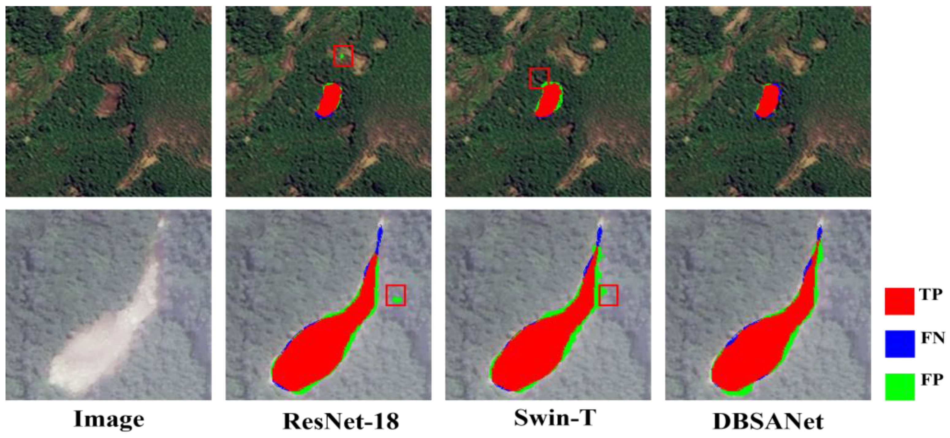
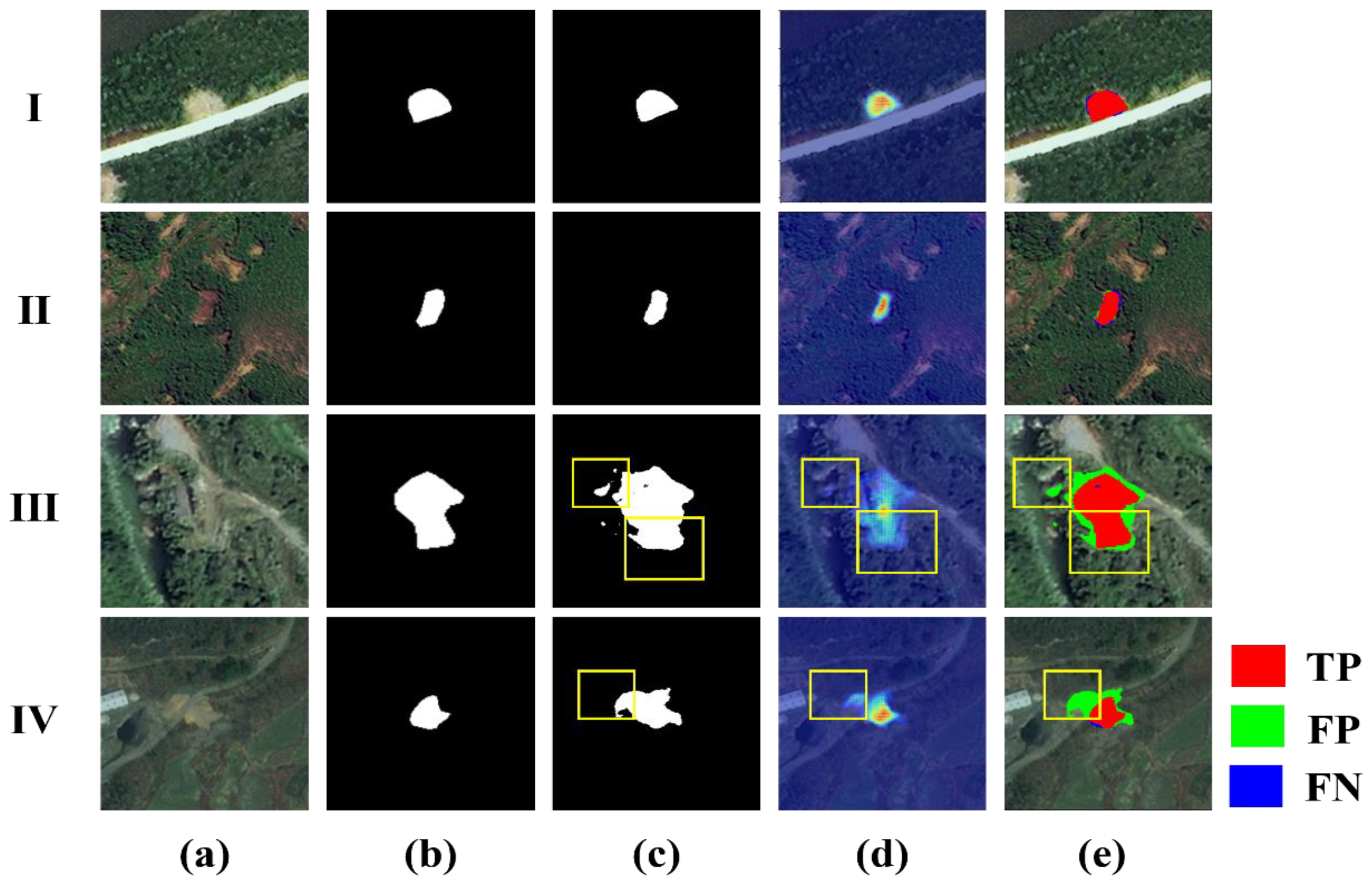
Table 6 present the experimental results for various models evaluated on the Bijie dataset and the Luding dataset. The data clearly indicate that DBSANet outperforms all other models across the three performance metrics. Specifically, compared to the other seven models for comparison, DBSANet exhibits average enhancements of 4.91% in the IoU, 0.57% in the accuracy, and 3.25% in the F1_score. Likewise, on the Luding dataset, DBSANet displays exceptional performance, demonstrating average improvements of 2.96%, 1.08%, and 1.97% in the IoU, accuracy, and F1_score, respectively. It has achieved superior performance on both the Bijie and Luding datasets, further suggesting that our model can more precisely align the overlapping regions between the actual and predicted landslide areas during detection. This not only reduces the false alarm rate, defined as the incorrect identification of non-landslide areas as landslide areas, but also lowers the missed detection rate, which refers to the failure to identify actual landslide regions. To visually compare the landslide detection performance of DBSANet with other models, we visualized the prediction outcomes for each model, as depicted in Figure 12 and Figure 13. The figure clearly illustrates that true positives (TPs) dominate the area in the DBSANet visualization results, while false positives (FPs) and false negatives (FNs) occupy comparatively smaller areas, thereby effectively demonstrating the network’s efficacy in the landslide detection task.
In the experiments conducted on the Bijie dataset, ResUNet exhibited a superior performance among the CNN-based models when compared to UNet and Deeplabv3+, indicating that the adoption of the ResNet structure can achieve a better feature representation on the Bijie dataset. Compared to traditional CNN-based methods, SwinUNet introduces a self-attention mechanism for feature extraction. Although it adopts a similar network structure to UNet, its relatively simple network architecture somewhat limits its performance in landslide detection tasks. As a consequence, its overall performance falls short when compared to other benchmark models. The segmentation results depicted in Figure 12 reveal a degree of boundary blurring in the landslide region when using SwinUNet. This observation suggests that SwinUNet’s reliance on a self-attention mechanism for global information interaction, in contrast to CNNs, might compromise the precision of local detail processing. Conversely, TransUNet, TransFuse, and UNetFormer adeptly amalgamate the CNN’s and Transformer’s strengths, albeit through distinct integration strategies. TransUNet employs a hybrid encoder strategy. Initially, CNNs are utilized for feature extraction, followed by partitioning the resulting feature maps into patches and transforming them into one-dimensional vectors. These vectors are then integrated into the Transformer framework to enhance global comprehension. In contrast, TransFuse concurrently processes the CNN’s and Transformer’s features, employing novel fusion techniques to effectively amalgamate features derived from parallel branches. UNetFormer follows a structure akin to UNet but enhances the fusion of global and local information by substituting the decoder with a Transformer. These hybrid models demonstrated significant improvements in IoU metrics—5.78%, 6.58%, and 7.44%, respectively—compared to SwinUNet’s pure Transformer architecture, underscoring the efficacy of hybrid model architectures in landslide detection tasks. In comparison to the previously mentioned CNN-based models, pure Transformer architecture models, and hybrid models, DBSANet, as proposed in this study, demonstrates notable performance advantages in the context of landslide detection tasks. More specifically, when compared to the top-performing models within each respective category (ResUNet, SwinUNet, and UNetFormer), DBSANet exhibits improvements of 2.38%, 10.81%, and 3.37% in the IoU metric performance, thus unequivocally showcasing DBSANet’s superiority in the realm of landslide detection tasks.
In the Luding dataset experiments, while comparison models like UNet stand out among CNN-based models and UNetFormer achieves the top performance among the CNN and Transformer hybrid models, their evaluation metrics still do not surpass those of DBSANet proposed in this study. Particularly noteworthy is that, compared to the top-performing model in each category, the DBSANet proposed in this study has achieved improvements in the IoU values of 2.19%, 2.66%, and 2.47%, respectively. This underscores the broad applicability of DBSANet across various landslide datasets and its efficacy in landslide detection.

4.2. Comparison of Model Efficiency

To facilitate a clear comparison of computational efficiency among different models, this study quantifies the computational efficiency based on the model parameters, average training time for each epoch, and inference speed per image, with the experimental results detailed in Table 7. As illustrated in the table, DBSANet does not lead to excessive memory consumption; however, it is worth noting that the dual-branch structure adopted by the model also enhances the training time of the model to some extent. Compared to models based on CNNs or pure Transformer structures, DBSANet makes a trade-off between efficiency and accuracy, but leans more towards the latter. Furthermore, in contrast to the hybrid model, DBSANet attains superior results in landslide detection using fewer parameters.

4.3. Application of DBSANet in Other Scenarios

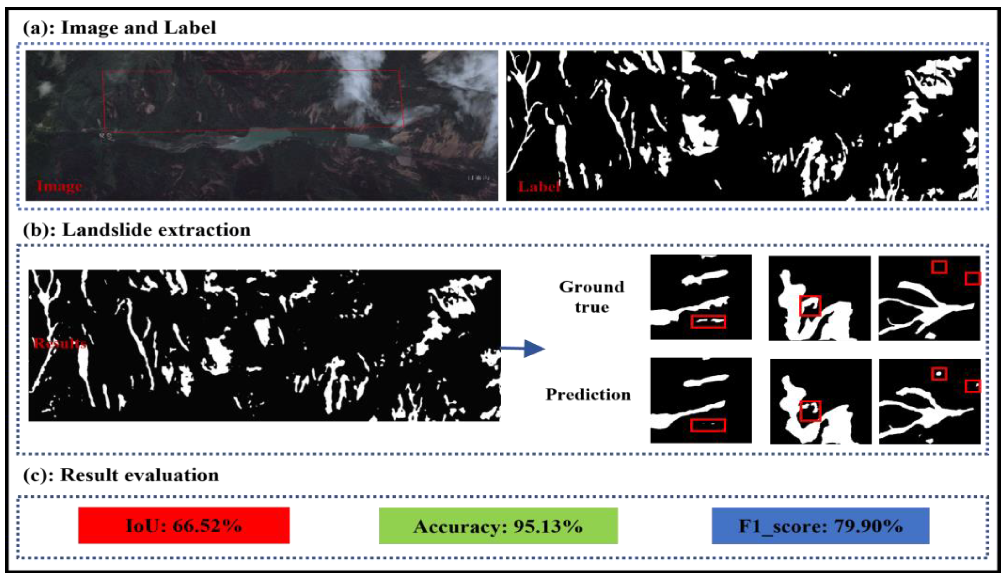
In order to further validate the generalization of the DBSANet model, we identified the Rizhaigou watershed in Jiuzhaigou County as the experimental site. The region’s abundant rainfall, in conjunction with its intricate geological formations, frequently precipitates the occurrence of landslides alongside the rivers. In the preliminary phase of the experiment, we successfully obtained landslide samples from this area by combining GF-2 satellite imagery with Google Earth imagery through visual interpretation. Subsequently, building upon the training results from the Luding dataset, we fine-tuned the model and performed an extensive evaluation on GF-2 imagery obtained from the Rizhaigou watershed. The experimental results are shown in Figure 14.
As illustrated in the figure, the DBSANet model effectively identified the majority of landslide areas within the experimental region. Specifically, the model’s performance metrics were as follows: the IoU was 66.52%, the accuracy was 95.13%, and the F1-score was 79.90%. However, it is important to note that while these metrics reflect a certain performance level, they have not yet reached optimal levels. This is primarily due to the fact that applying a trained model to an unexplored region presents a considerable challenge. Most prior studies have conducted training and validation within the same region, thus avoiding challenges such as geological structure disparities and variations in image features. In contrast, the images in the Luding dataset were captured shortly after an earthquake, displaying notable differences from the test images of the Rizhaigou watershed (acquired in May 2023). Furthermore, as observed in the prediction results presented in Figure 14, the DBSANet model erroneously classified non-landslide areas as landslides in some instances (indicated by red boxes). This misidentification may arise from two primary factors: first, the manual labeling of landslide tags inherently involves subjectivity, and labeling errors may lead the model to acquire erroneous information; second, the majority of landslides in the Rizhaigou watershed are aged, and the vegetation on the slopes has developed over an extended period, causing the landslide boundaries to become blurred and difficult to define accurately. This alteration in vegetation cover undoubtedly exacerbates the challenges associated with landslide detection. In summary, while the DBSANet model has shown the capacity to accurately identify landslide positions in other application contexts, the experimental results from the Rizhaigou watershed show that the model still requires improvement in determining the specific scope of landslides.

4.4. Limitations and Future Work

The DBSANet model employs a dual-branch parallel structure consisting of a ResNet and Swin Transformer as its encoder. The Swin Transformer branch effectively captures long-range dependencies across various regions of the image, whereas the ResNet branch extracts local feature information, thereby facilitating the model’s acquisition of more comprehensive feature representations. From Table 5 and Table 6, it is evident that the model demonstrates a substantial enhancement in landslide detection performance. However, the analysis of Figure 10 and Figure 11 reveals the difficulties associated with accurately delineating the extent of landslides, particularly when they are incomplete, such as during the emergence of nascent vegetation. This limitation can be attributed to the restricted sample size of the landslide dataset employed in this study, which impedes the model’s ability to represent all possible types of landslides. Consequently, the emergence of new vegetation on the landslide surface presents a significant challenge for the model, hindering its ability to precisely delineate the landslide boundaries.
In future research, we will gather landslide data across various scenarios to enhance the diversity of features available for model training. Furthermore, to improve the generalizability and adaptability of the model across various application scenarios, we will integrate a diverse range of multi-source remote sensing data—including, but not limited to, digital elevation models, and slope information—into the dataset construction, which is anticipated to further enhance the model’s performance in real-world contexts, given the substantial influence of these factors on landslide occurrences.

5. Conclusions

In this study, we propose a semantic segmentation model named DBSANet, which is based on a U-shaped encoder–decoder architecture for landslide detection in remote sensing images. Inspired from the Transformer’s global modeling via self-attention and the CNN’s adept feature extraction capabilities, the DBSANet encoder integrates a dual-branch parallel structure of a Transformer and CNN. This design facilitates the concurrent acquisition of both comprehensive contextual information and low-level spatial details of images. Given the inherent structural disparities in feature representations between the CNN and Transformer during extraction, we propose an FFM designed to merge features from both branches, thereby effectively integrating their complementary attributes. Additionally, in order to bridge the semantic gap between the encoder and decoder and thereby enhance the overall model performance, we design an SGAM integrated within the skip connection segment. This module aims to heighten the model’s emphasis on pivotal areas by aligning the decoder feature maps with those of the encoder, effectively bridging the semantic gap between them. To thoroughly and systematically assess the criticality of each module within the model, we carefully designed and executed a series of ablation experiments. The final results of the experiments unequivocally demonstrate that these modules play indispensable roles. To further verify the efficacy and generalizability of DBSANet, experiments were performed on the Bijie and Luding datasets. The experimental results demonstrated that DBSANet markedly exceeded the performance of the other comparative models in terms of the semantic segmentation accuracy. This further demonstrates that the meticulously designed DBSANet in this study effectively integrates the advantages of CNNs and Transformers, thereby enhancing the accuracy of landslide detection, and also provides substantial technical support for the deployment of the hybrid model in landslide detection applications.
Although the remarkable performance exhibited by DBSANet in a variety of experiments is impressive, two limitations persist. First, the incorporation of a dual-branch encoder inherently leads to an increase in the number of parameters, thereby extending the training duration. Second, in scenarios where the surface of landslide bodies is obscured by emerging vegetation, DBSANet encounters difficulties in precisely delineating the landslide boundaries. To address these limitations, future research will concentrate on enhancing efficiency while preserving high accuracy, and applying this equilibrium to landslide detection tasks. Furthermore, we plan to explore ways to integrate multi-source data into the landslide detection process, ensuring that the model can effectively learn and extract crucial features in diverse, complex scenarios, thereby enhancing the recognition of landslide boundaries and improving the model’s generalization performance.

Author Contributions

All the authors made significant contributions to this work. Conceptualization, W.Z. and Y.L.; methodology, W.Z. and Y.L.; software and experiments, Y.L.; validation, J.W., R.Z. and Y.Z.; writing—original draft preparation, Y.L.; writing—review and editing, W.Z. and X.X.; supervision, Y.Z.; funding acquisition, W.Z. and X.X. All authors have read and agreed to the published version of the manuscript.

Funding

This research was funded by the National Key R&D Program of China (2023YFC3008402), Natural Science Foundation of China (NSFC) (Nos.: 42474051, 42074040), Natural Science Basic Research Plan in Shaanxi Province of China (Nos.: 2023-JC-JQ-24, 2022JQ-454), the innovation team of Shaanxi Provincial Tri-Qin Scholars with Geoscience Big Data and Geohazard Prevention (2022), Fundamental Research Funds for the Central Universities of CHD (Nos.: 300102263401, 300102264502, 300102264915).

Data Availability Statement

The Bijie dataset used in this study can be obtained from the Bijie Landslide Dataset (whu.edu.cn), accessed on 30 March 2024. The satellite imagery data involved in the study can be acquired from the China Center for Resources Satellite Data and Application at https://www.cresda.com/zgzywxyyzx/index.html, accessed on 1 November 2024.

Acknowledgments

The authors would like to express their sincere gratitude to the reviewers and editors for their constructive and high-quality revision suggestions on this manuscript.

Conflicts of Interest

The authors declare no conflicts of interest.

References

  1. Zhu, W.; Yang, L.Y.; Cheng, Y.Q.; Liu, X.Y.; Zhang, R.X. Active thickness estimation and failure simulation of translational landslide using multi-orbit InSAR observations: A case study of the Xiongba landslide. Int. J. Appl. Earth Obs. Geoinf. 2024, 129, 16. [Google Scholar] [CrossRef]
  2. Pardeshi, S.D.; Autade, S.E.; Pardeshi, S.S. Landslide hazard assessment: Recent trends and techniques. SpringerPlus 2013, 2, 523. [Google Scholar] [CrossRef] [PubMed]
  3. Zhang, J.M.; Zhu, W.; Cheng, Y.Q.; Li, Z.H. Landslide Detection in the Linzhi-Ya’an Section along the Sichuan-Tibet Railway Based on InSAR and Hot Spot Analysis Methods. Remote Sens. 2021, 13, 3566. [Google Scholar] [CrossRef]
  4. Wang, C.S.; Chang, L.; Wang, X.S.; Zhang, B.C.; Stein, A. Interferometric Synthetic Aperture Radar Statistical Inference in Deformation Measurement and Geophysical Inversion: A review. IEEE Geosci. Remote Sens. Mag. 2024, 12, 8–35. [Google Scholar] [CrossRef]
  5. Zhang, R.-X.; Zhu, W.; Li, Z.-H.; Zhang, B.-C.; Chen, B. Re-Net: Multibranch Network With Structural Reparameterization for Landslide Detection in Optical Imagery. IEEE J. Sel. Top. Appl. Earth Obs. Remote Sens. 2024, 17, 2828–2837. [Google Scholar] [CrossRef]
  6. Ansari, M.D.; Ghrera, S.; Tyagi, V. Pixel-Based Image Forgery Detection: A Review. IETE J. Educ. 2014, 55, 40–46. [Google Scholar] [CrossRef]
  7. Ghorbanzadeh, O.; Gholamnia, K.; Ghamisi, P. The application of ResU-net and OBIA for landslide detection from multi-temporal sentinel-2 images. Big Earth Data 2023, 7, 961–985. [Google Scholar] [CrossRef]
  8. Shi, W.Z.; Zhang, M.; Ke, H.F.; Fang, X.; Zhan, Z.; Chen, S.X. Landslide Recognition by Deep Convolutional Neural Network and Change Detection. IEEE Trans. Geosci. Remote Sens. 2021, 59, 4654–4672. [Google Scholar] [CrossRef]
  9. Cheng, L.B.; Li, J.; Duan, P.; Wang, M.G. A small attentional YOLO model for landslide detection from satellite remote sensing images. Landslides 2021, 18, 2751–2765. [Google Scholar] [CrossRef]
  10. Ullo, S.L.; Mohan, A.; Sebastianelli, A.; Ahamed, S.E.; Kumar, B.; Dwivedi, R.; Sinha, G. A New Mask R-CNN-Based Method for Improved Landslide Detection. IEEE J. Sel. Top. Appl. Earth Obs. Remote Sens. 2021, 14, 3799–3810. [Google Scholar] [CrossRef]
  11. Noh, H.; Hong, S.; Han, B. Learning Deconvolution Network for Semantic Segmentation. In Proceedings of the IEEE International Conference on Computer Vision, Santiago, Chile, 11–18 December 2015; pp. 1520–1528. [Google Scholar]
  12. Yi, Y.; Zhang, W. A New Deep-Learning-Based Approach for Earthquake-Triggered Landslide Detection From Single-Temporal RapidEye Satellite Imagery. IEEE J. Sel. Top. Appl. Earth Obs. Remote Sens. 2020, 13, 6166–6176. [Google Scholar] [CrossRef]
  13. Prakash, N.; Manconi, A.; Loew, S. Mapping Landslides on EO Data: Performance of Deep Learning Models vs. Traditional Machine Learning Models. Remote Sens. 2020, 12, 346. [Google Scholar] [CrossRef]
  14. Long, J.; Shelhamer, E.; Darrell, T. Fully Convolutional Networks for Semantic Segmentation. In Proceedings of the IEEE Conference on Computer Vision and Pattern Recognition (CVPR), Boston, MA, USA, 7–12 June 2015; pp. 3431–3440. [Google Scholar]
  15. He, K.M.; Zhang, X.Y.; Ren, S.Q.; Sun, J. Deep Residual Learning for Image Recognition. In Proceedings of the 2016 IEEE Conference on Computer Vision and Pattern Recognition (CVPR), Seattle, WA, USA, 27–30 June 2016; pp. 770–778. [Google Scholar]
  16. Meena, S.R.; Soares, L.P.; Grohmann, C.H.; van Westen, C.; Bhuyan, K.; Singh, R.P.; Floris, M.; Catani, F. Landslide detection in the Himalayas using machine learning algorithms and U-Net. Landslides 2022, 19, 1209–1229. [Google Scholar] [CrossRef]
  17. Li, Z.; Guo, Y. Semantic segmentation of landslide images in Nyingchi region based on PSPNet network. In Proceedings of the 2020 7th International Conference on Information Science and Control Engineering (ICISCE), Changsha, China, 8–20 December 2020; pp. 1269–1273. [Google Scholar]
  18. Qi, W.W.; Wei, M.F.; Yang, W.T.; Xu, C.; Ma, C. Automatic Mapping of Landslides by the ResU-Net. Remote Sens. 2020, 12, 2487. [Google Scholar] [CrossRef]
  19. Chen, L.-C.; Zhu, Y.; Papandreou, G.; Schroff, F.; Adam, H. Encoder-Decoder with Atrous Separable Convolution for Semantic Image Segmentation. In Proceedings of the 15th European Conference on Computer Vision, Munich, Germany, 8–14 September 2018; Proceedings, Part VII. pp. 833–851. [Google Scholar]
  20. Xia, W.; Chen, J.; Liu, J.B.; Ma, C.H.; Liu, W. Landslide Extraction from High-Resolution Remote Sensing Imagery Using Fully Convolutional Spectral-Topographic Fusion Network. Remote Sens. 2021, 13, 5116. [Google Scholar] [CrossRef]
  21. Chen, H.S.; He, Y.; Zhang, L.F.; Yao, S.; Yang, W.; Fang, Y.M.; Liu, Y.X.; Gao, B.H. A landslide extraction method of channel attention mechanism U-Net network based on Sentinel-2A remote sensing images. Int. J. Digit. Earth 2023, 16, 552–577. [Google Scholar] [CrossRef]
  22. Zhou, Z.W.; Siddiquee, M.M.R.; Tajbakhsh, N.; Liang, J.M. UNet plus plus: Redesigning Skip Connections to Exploit Multiscale Features in Image Segmentation. IEEE Trans. Med. Imaging 2020, 39, 1856–1867. [Google Scholar] [CrossRef]
  23. Pang, Y.W.; Li, Y.Z.; Shen, J.B.; Shao, L. Towards Bridging Semantic Gap to Improve Semantic Segmentation. In Proceedings of the IEEE/CVF International Conference on Computer Vision (ICCV), Seoul, Republic of Korea, 27 October–2 November 2019; pp. 4229–4238. [Google Scholar]
  24. Vaswani, A.; Shazeer, N.; Parmar, N.; Uszkoreit, J.; Jones, L.; Gomez, A.N.; Kaiser, L.; Polosukhin, I. Attention Is All You Need. In Proceedings of the 31st Annual Conference on Neural Information Processing Systems (NIPS), Long Beach, CA, USA, 4–9 December 2017. [Google Scholar]
  25. Cao, H.; Wang, Y.; Chen, J.; Jiang, D.; Zhang, X.; Tian, Q.; Wang, M. Swin-Unet: Unet-Like Pure Transformer for Medical Image Segmentation; Springer: Cham, Switzerland, 2021. [Google Scholar]
  26. Chen, J.; Lu, Y.; Yu, Q.; Luo, X.; Adeli, E.; Wang, Y.; Lu, L.; Yuille, A.L.; Zhou, Y. TransUNet: Transformers Make Strong Encoders for Medical Image Segmentation. arXiv 2021, arXiv:2102.04306. [Google Scholar]
  27. Zhang, Y.D.; Liu, H.Y.; Hu, Q. TransFuse: Fusing Transformers and CNNs for Medical Image Segmentation. In Proceedings of the International Conference on Medical Image Computing and Computer Assisted Intervention (MICCAI), Strasbourg, France, 27 September–1 October 2021; pp. 14–24. [Google Scholar]
  28. Wang, L.B.; Li, R.; Zhang, C.; Fang, S.H.; Duan, C.X.; Meng, X.L.; Atkinson, P.M. UNetFormer: A UNet-like transformer for efficient semantic segmentation of remote sensing urban scene imagery. ISPRS-J. Photogramm. Remote Sens. 2022, 190, 196–214. [Google Scholar] [CrossRef]
  29. Lv, P.Y.; Ma, L.S.; Li, Q.M.; Du, F. ShapeFormer: A Shape-Enhanced Vision Transformer Model for Optical Remote Sensing Image Landslide Detection. IEEE J. Sel. Top. Appl. Earth Obs. Remote Sens. 2023, 16, 2681–2689. [Google Scholar] [CrossRef]
  30. Tang, X.C.; Tu, Z.H.; Wang, Y.; Liu, M.Z.; Li, D.F.; Fan, X.M. Automatic Detection of Coseismic Landslides Using a New Transformer Method. Remote Sens. 2022, 14, 2884. [Google Scholar] [CrossRef]
  31. Azad, R.; Heidari, M.; Wu, Y.L.; Merhof, D. Contextual Attention Network: Transformer Meets U-Net. In Proceedings of the 13th International Workshop on Machine Learning in Medical Imaging (MLMI), Singapore, 18 September 2022; pp. 377–386. [Google Scholar]
  32. Xiang, X.Y.; Gong, W.P.; Li, S.L.; Chen, J.; Ren, T.H. TCNet: Multiscale Fusion of Transformer and CNN for Semantic Segmentation of Remote Sensing Images. IEEE J. Sel. Top. Appl. Earth Obs. Remote Sens. 2024, 17, 3123–3136. [Google Scholar] [CrossRef]
  33. Li, J.; Zhang, J.; Fu, Y.Y. CTHNet: A CNN-Transformer Hybrid Network for Landslide Identification in Loess Plateau Regions Using High-Resolution Remote Sensing Images. Sensors 2025, 25, 273. [Google Scholar] [CrossRef] [PubMed]
  34. Yang, Z.Q.; Xu, C.; Li, L. Landslide Detection Based on ResU-Net with Transformer and CBAM Embedded: Two Examples with Geologically Different Environments. Remote Sens. 2022, 14, 2885. [Google Scholar] [CrossRef]
  35. Ji, S.P.; Yu, D.W.; Shen, C.Y.; Li, W.L.; Xu, Q. Landslide detection from an open satellite imagery and digital elevation model dataset using attention boosted convolutional neural networks. Landslides 2020, 17, 1337–1352. [Google Scholar] [CrossRef]
  36. Liu, Z.; Lin, Y.T.; Cao, Y.; Hu, H.; Wei, Y.X.; Zhang, Z.; Lin, S.; Guo, B.N. Swin Transformer: Hierarchical Vision Transformer using Shifted Windows. In Proceedings of the 18th IEEE/CVF International Conference on Computer Vision (ICCV), 11–17 October 2021; pp. 9992–10002. [Google Scholar]
  37. Jiang, L.; Zhang, C.; Huang, M.; Liu, C.; Shi, J.; Loy, C.C. TSIT: A Simple and Versatile Framework for Image-to-Image Translation. In Proceedings of the Computer Vision–ECCV 2020: 16th European Conference, Glasgow, UK, 23–28 August 2020; pp. 206–222. [Google Scholar]
  38. Wang, X.T.; Yu, K.; Dong, C.; Loy, C.C. Recovering Realistic Texture in Image Super-resolution by Deep Spatial Feature Transform. In Proceedings of the 31st IEEE/CVF Conference on Computer Vision and Pattern Recognition (CVPR), Salt Lake City, UT, USA, 18–23 June 2018; pp. 606–615. [Google Scholar]
  39. Lee, H.; Kim, H.E.; Nam, H. SRM: A Style-based Recalibration Module for Convolutional Neural Networks. In Proceedings of the IEEE/CVF International Conference on Computer Vision (ICCV), Seoul, Republic of Korea, 27 October–2 November 2019; pp. 1854–1862. [Google Scholar]
  40. Howard, A.; Zhu, M.; Chen, B.; Kalenichenko, D.; Wang, W.; Weyand, T.; Andreetto, M.; Adam, H. MobileNets: Efficient Convolutional Neural Networks for Mobile Vision Applications. arXiv 2017, arXiv:1704.04861. [Google Scholar] [CrossRef]
  41. Keyport, R.N.; Oommen, T.; Martha, T.R.; Sajinkumar, K.S.; Gierke, J.S. A comparative analysis of pixel- and object-based detection of landslides from very high-resolution images. Int. J. Appl. Earth Obs. Geoinf. 2018, 64, 1–11. [Google Scholar] [CrossRef]
  42. Phan, T.H.; Yamamoto, K. Resolving Class Imbalance in Object Detection with Weighted Cross Entropy Losses. arXiv 2020, arXiv:2006.01413. [Google Scholar]
  43. Milletari, F.; Navab, N.; Ahmadi, S.A. V-Net: Fully Convolutional Neural Networks for Volumetric Medical Image Segmentation. In Proceedings of the 4th IEEE International Conference on 3D Vision (3DV), Stanford, CA, USA, 25–28 October 2016; pp. 565–571. [Google Scholar]
  44. Kingma, D.; Ba, J. Adam: A Method for Stochastic Optimization. In Proceedings of the International Conference on Learning Representations, Banff, AB, Canada, 14–16 April 2014. [Google Scholar]
  45. Selvaraju, R.R.; Cogswell, M.; Das, A.; Vedantam, R.; Parikh, D.; Batra, D. Grad-CAM: Visual Explanations from Deep Networks via Gradient-based Localization. In Proceedings of the 16th IEEE International Conference on Computer Vision (ICCV), Venice, Italy, 22–29 October 2017; pp. 618–626. [Google Scholar]
Figure 1. The coverage of the collected dataset.
Remotesensing 17 00807 g001
Figure 2. Structure of the proposed DBSANet.
Remotesensing 17 00807 g002
Figure 3. (a) Transformer block. (b) Swin Transformer Block.
Remotesensing 17 00807 g003
Figure 4. Example of feature map visualization in the Luding dataset, where Stage 1, Stage 2, Stage 3, and Stage 4 correspond to the four stages of feature extraction for the four backbone encoders (any two output channels). The feature maps are depicted using COLORMAP_JET pseudocolors to enhance visual differentiation. The COLORBAR is on the rightmost side of the figure, and the pixel values correspond to the colors increasing from bottom to top.
Remotesensing 17 00807 g004
Figure 5. Structure of the proposed FFM.
Remotesensing 17 00807 g005
Figure 6. Structure of the proposed SGAM.
Remotesensing 17 00807 g006
Figure 7. Visualization of confusion matrix statistics for the Bijie and Luding datasets.
Remotesensing 17 00807 g007
Figure 8. An example of the feature map COLORMAP_JET pseudocolor visualization in the Luding dataset, where Stage 1, Stage 2, Stage 3, and Stage 4 correspond to the four stages of feature extraction for the four backbone encoders (any two output channels).
Remotesensing 17 00807 g008
Figure 9. Bijie dataset image Grad-CAM visualization (c,d) and COLORMAP_JET pseudocolor visualization (e,h). (a) Image. (b) Label. (c) Grad-CAM visualization of DBSANet (without SGAM) output layer. (d) Grad-CAM visualization of DBSANet output layer. (e) DBSANet Encoder Stage 1 output channel visualization. (f) Decoder output channel visualization corresponding to Stage 1 in DBSANet. (g) DBSANet (without SGAM) output channel visualization. (h) DBSANet output channel visualization.
Remotesensing 17 00807 g009
Figure 10. Test results of DBSANet on Bijie test set (IIV are four example images in the test set). (a) Image. (b) Label. (c) DBSANet segmentation result. (d) Grad-CAM visualization of DBSANet’s output layer. (e) Visualization of confusion matrix statistics. TP denotes the number of pixels accurately identified as landslides; FP denotes the number of pixels where the background is incorrectly recognized as a landslide; and FN denotes the number of pixels where the landslide is incorrectly recognized as background.
Remotesensing 17 00807 g010
Figure 11. Test results of DBSANet on Luding test set (IIV are four example images in the test set). (a) Image. (b) Label. (c) DBSANet segmentation result. (d) Grad-CAM visualization of DBSANet’s output layer. (e) Visualization of confusion matrix statistics. TP denotes the number of pixels accurately identified as landslides; FP denotes the number of pixels where the background is incorrectly recognized as a landslide; and FN denotes the number of pixels where the landslide is incorrectly recognized as background.
Remotesensing 17 00807 g011
Figure 12. Visualization of confusion matrix statistics for the Bijie dataset.
Remotesensing 17 00807 g012
Figure 13. Visualization of confusion matrix statistics for the Luding dataset.
Remotesensing 17 00807 g013
Figure 14. Application of DBSANet in other scenarios.
Remotesensing 17 00807 g014
Table 1. Comparisons of the two-branch encoder ablation experiment.
DatasetModelIoUAccuracyF1_Score
BijieResNet-1874.08%97.21%85.11%
Swin-T72.67%97.01%84.17%
DBSANet77.12%97.60%87.08%
LudingResNet-1872.44%91.86%84.02%
Swin-T73.92%92.42%85.00%
DBSANet75.23%92.97%85.87%
Table 2. Ablation experiment results of FFM.
DatasetModelIoUAccuracyF1_Score
BijieBaseline72.91%97.12%84.34%
Baseline + FFM75.63%97.44%86.13%
DBSANet (no FFM)74.20%97.30%85.19%
DBSANet77.12%97.60%87.08%
LudingBaseline71.74%91.65%83.55%
Baseline + FFM72.95%91.90%84.36%
DBSANet (no FFM)73.73%92.54%84.88%
DBSANet75.23%92.97%85.87%
Table 3. Ablation experiment results of SGAM.
DatasetModelIoUAccuracyF1_Score
BijieBaseline72.91%97.12%84.34%
Baseline + SGAM74.20%97.30%85.19%
DBSANet (no SGAM)75.63%97.44%86.13%
DBSANet77.12%97.60%87.08%
LudingBaseline71.74%91.65%83.55%
Baseline + SGAM73.73%92.54%84.88%
DBSANet (no SGAM)72.95%91.90%84.36%
DBSANet75.23%92.97%85.87%
Table 4. Accuracy of DBSANet in Bijie and Luding datasets.
DatasetIoUAccuracyF1_Score
Bijie77.12%97.60%87.08%
Luding75.23%92.97%85.87%
Table 5. Comparisons of accuracy among various models on the Bijie dataset.
ModelIoUAccuracyF1_Score
UNet73.93%97.20%85.01%
Deeplabv3+71.74%97.07%83.55%
ResUNet74.74%97.36%85.55%
SwinUNet66.31%96.22%79.74%
TransUNet72.09%97.08%83.78%
TransFuse72.89%97.06%84.32%
UNetFormer73.75%97.19%84.89%
DBSANet77.12%97.60%87.08%
Table 6. Comparisons of accuracy among various models on the Luding dataset.
ModelIoUAccuracyF1_Score
UNet73.04%91.96%84.42%
Deeplabv3+70.75%91.36%82.87%
ResUNet72.20%92.03%83.86%
SwinUNet72.57%92.06%84.10%
TransUNet72.04%91.85%83.75%
TransFuse72.50%91.93%84.06%
UNetFormer72.76%92.02%84.23%
DBSANet75.23%92.97%85.87%
Table 7. Comparisons of parameters and inference speed among various models.
ModelParameters (M)Average Training Time (s/Epoch)Inference Speed (ms/Image)
UNet17.2320.734.85
Deeplabv3+59.3420.766.10
ResUNet48.5514.335.28
Swin_UNet27.1915.064.18
TransUNet51.0722.415.17
TransFuse98.4924.067.87
UNetFormer21.8315.583.02
Ours39.9825.566.69
Disclaimer/Publisher’s Note: The statements, opinions and data contained in all publications are solely those of the individual author(s) and contributor(s) and not of MDPI and/or the editor(s). MDPI and/or the editor(s) disclaim responsibility for any injury to people or property resulting from any ideas, methods, instructions or products referred to in the content.

