Article

The Spatiotemporal Evolution and Driving Forces of the Urban Heat Island in Shijiazhuang

1
Hebei Key Laboratory of Optoelectronic Information and Geo-detection Technology, Hebei GEO University, Shijiazhuang 050031, China
2
Hebei Center for Ecological and Environmental Geology Research, Hebei GEO University, Shijiazhuang 050031, China
3
Hebei International Joint Research Center for Remote Sensing of Agricultural Drought Monitoring, Hebei GEO University, Shijiazhuang 050031, China
4
State Key Laboratory of Resources and Environment Information System, Institute of Geographic Sciences and Natural Resources Research, Chinese Academy of Sciences, Beijing 100101, China
*
Author to whom correspondence should be addressed.
Remote Sens. 2025, 17(5), 781; https://doi.org/10.3390/rs17050781
Submission received: 3 January 2025 / Revised: 8 February 2025 / Accepted: 21 February 2025 / Published: 23 February 2025

Abstract

:
As a comprehensive reflection of the thermal characteristics of the urban environment, the urban heat island (UHI) effect has triggered a series of ecological and environmental issues. Existing studies on the UHI effect in Shijiazhuang, the capital of Hebei Province, China, have primarily focused on spatial–temporal distribution characteristics and migration trends, with less focus on the influences of other contributing factors. This study focuses on Shijiazhuang city, using Landsat ETM+/OLI data from 2000 to 2020 to analyze the spatiotemporal traits of the UHI effect. The mono-window algorithm (MW) was used to retrieve land surface temperatures (LSTs), and the seasonal autoregressive integrated moving average (SARIMA) model was used to predict LST trends. Key factors such as the normalized difference vegetation index (NDVI), digital elevation model (DEM), population (POP), precipitation (PPT), impervious surface (IPS), potential evapotranspiration (PET), particulate matter 2.5 (PM2.5), and night light (NL) were analyzed using spatial autocorrelation to explore their dynamic relationship with the UHI. Specifically, a multi-scale analysis model was developed to search for the optimum urban spatial scale, enabling a comprehensive assessment of the spatiotemporal evolution and drivers of the UHI in Shijiazhuang. The UHI showed pronounced spatial clustering, expanding annually by 44.288 km2, with a southeastward shift. Autumn exhibited the greatest reduction in UHI, while predictions suggested peak temperatures in summer 2027. According to the bivariate clustering analysis, the NDVI was the most influential factor in mitigating the UHI, while the IPS spatially showed the most significant enhancement in the UHI in the central urban areas. Other factors generally promoted the UHI after 2005. The multi-scale geographically weighted regression (MGWR) model was best fitted at a 3 km × 3 km scale. Considering the joint effects of multiple factors, the ranking of contributing factors to the model prediction is as follows: PET > DEM > NDVI > IPS > PPT > PM2.5 > NL > POP. The interactive effects, especially between the PET and DEM, reach a significant value of 0.72. These findings may address concerns regarding both future trends and mitigation indications for UHI variations in Shijiazhuang.

1. Introduction

Since Howard first reported the UHI phenomenon in London in 1833, this topic has garnered widespread attention from various fields [1]. The urban heat island effect refers to the phenomenon where urban areas exhibit higher air or surface temperatures compared to their surrounding rural areas [2]. Early studies focused on the impact of urbanization on local climates, while subsequent work examined the contribution of UHIs to global climate change [3]. The extent of urbanization, such as the increase in impervious surfaces and the reduction in vegetation, largely determines the severity of the UHI effect, as these factors alter the radiative balance of urban areas [4]. Impervious surfaces lead to reduced latent heat flux and increased sensible heat flux, while anthropogenic heat from sources such as traffic, industry, and buildings further amplifies this effect [5]. The UHI effect impacts energy consumption, particularly cooling loads, and can lead to increased cloud cover and precipitation [6]. It also plays a significant role in the atmospheric heat circulation over cities [7].
Recent studies on the spatiotemporal evolution of the UHI effect focus on understanding patterns, trends, and their relationships with urban planning and development through the urbanization process at multiple scales. Multi-temporal remote sensing data have been widely used to monitor and analyze the dynamics of UHIs. Studies in various regions, such as the Chang-Zhu-Tan urban agglomeration, Guangdong–Hong Kong–Macao Greater Bay Area, and Zhengzhou, have examined UHI characteristics and suggested appropriate methods for monitoring UHI patterns at different scales [8,9,10]. Broader analyses across regions, such as Jiangsu Province and Chinese urban agglomerations, employ statistical methods like redundancy analysis (RDA) and variance partitioning analysis (VPA) to reveal UHI mechanisms [11,12]. On a global scale, quantifications of UHIs across over a thousand cities from 2003 to 2019 underscore the spatial and temporal variations in UHI phenomena using the Dynamic Urban Extent (DUE) scheme [13].
Regarding UHI driving factors, extensive investigations have been executed on how urban structure and regional climate conditions influence UHI effects [14,15]. Long-term studies, such as those focusing on meteorological data in Chongqing, highlight the role of weather conditions in UHI dynamics [16]. Research on spatial heterogeneity and SUHI mechanisms in China offers insight into UHI formation across diverse urban settings [17]. However, while numerous studies have identified key drivers, there continue to be challenges in integrating datasets across scales and refining predictive models, particularly due to uncertainties in LST data under varying cloud conditions [18,19].
UHI research generally utilizes remote sensing data, statistical models, and GIS methodologies for comprehensive analysis of its spatiotemporal pattern and driving factors. Systematic reviews have underscored the critical importance of land surface temperature (LST) data and potential factors associated with urban morphology and land cover changes [20,21]. Common analytical approaches include remote sensing-based temperature retrieval techniques and GIS-based spatial analysis, which provide insights into UHI patterns and variations across urban landscapes. While data availability has significantly expanded, some researchers noted the need for more comprehensive simulation models to enhance predictive capacity and develop effective mitigation strategies in monitoring UHIs [22]. Furthermore, studies employing non-parametric models demonstrate that spatial methodologies are effective for representing complex spatial processes and interactions in UHI research [23]. Accurate LST data are essential for understanding UHI spatial heterogeneity and guiding mitigation strategies. Various algorithms have been developed for retrieving LSTs from thermal infrared data, including the single-channel method for ASTER, the SC-PM method for HJ-1B/IRS, and the split-window algorithm for AVHRR [24,25,26,27,28].
Current research on the urban heat island of Shijiazhuang focuses on the spatial and temporal distribution of and variation in the UHI, but there is still a gap in understanding the influence of various factors on its evolution. This study aims to analyze in detail the impacts of the UHI in Shijiazhuang, providing insights into future trends and their causes. This study utilizes Landsat data and applies the single-window algorithm to retrieve the LST. UHI changes are examined over a 20-year span by analyzing images from five time points between 2000 and 2020, along with detailed seasonal UHI analyses using images from each season from 2016 to 2020. Key factors—including the normalized difference vegetation index (NDVI), digital elevation model (DEM), population (POP), precipitation (PPT), impervious surface (IPS), potential evapotranspiration (PET), particulate matter 2.5 (PM2.5), and night light (NL)—are considered in the UHI attribution analysis. The results of this study will contribute to the formulation of effective policies to mitigate the impacts of the UHI and promote sustainable urban development in this critical region.

2. Materials and Methods

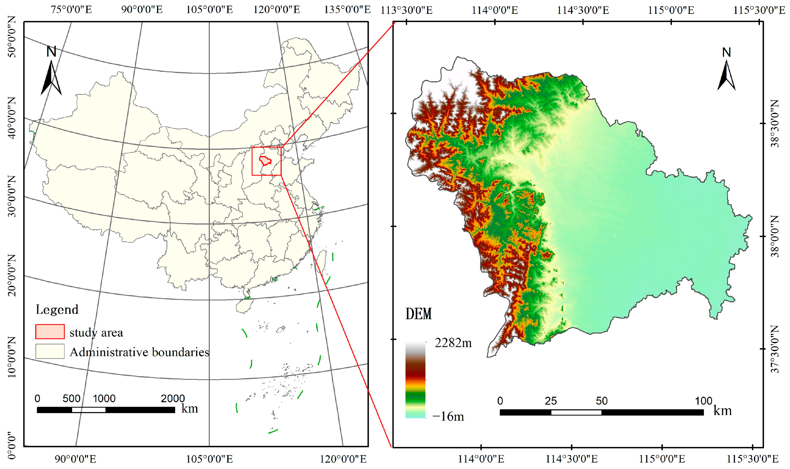
2.1. Description of the Study Area

Shijiazhuang, the capital city of Hebei Province, is a central hub within the Beijing–Tianjin–Hebei economic region, playing a vital role in regional development. It is strategically located approximately 280 km southwest of Beijing and covers an area of 15,848 km2 (Figure 1), positioning it as a key urban center in northern China.
As the capital of Hebei Province and a key city in the Beijing–Tianjin–Hebei region, Shijiazhuang holds strategic importance. Its political influence extends beyond Hebei, serving as a crucial liaison between the provincial government and the central government, especially in the context of regional integration efforts like the Beijing–Tianjin–Hebei coordinated development strategy and the establishment of the Xiong’an New Area [29]. Economically, Shijiazhuang is a driving force within Hebei Province, contributing significantly to the region’s Gross Domestic Product (GDP) through its diverse industrial base, which includes manufacturing, pharmaceuticals, and agriculture. Shijiazhuang’s rapid urbanization has brought notable economic and cultural progress, but it has also intensified environmental challenges, with the UHI effect becoming increasingly severe. This issue is exacerbated by population growth, industrialization, and increased building density, presenting new challenges for the urban environment and residents’ well-being. Despite its significance, the UHI effect in Shijiazhuang has not been extensively studied. Understanding the spatiotemporal patterns and drivers of the UHI effect in this city is critical, as it can inform regional policy-making and urban planning. The UHI effect, which reflects changes in urban thermal environments, influences the regional climate, air quality, and urban ecosystems, leading to various ecological and environmental challenges.

2.2. Multi-Source Data
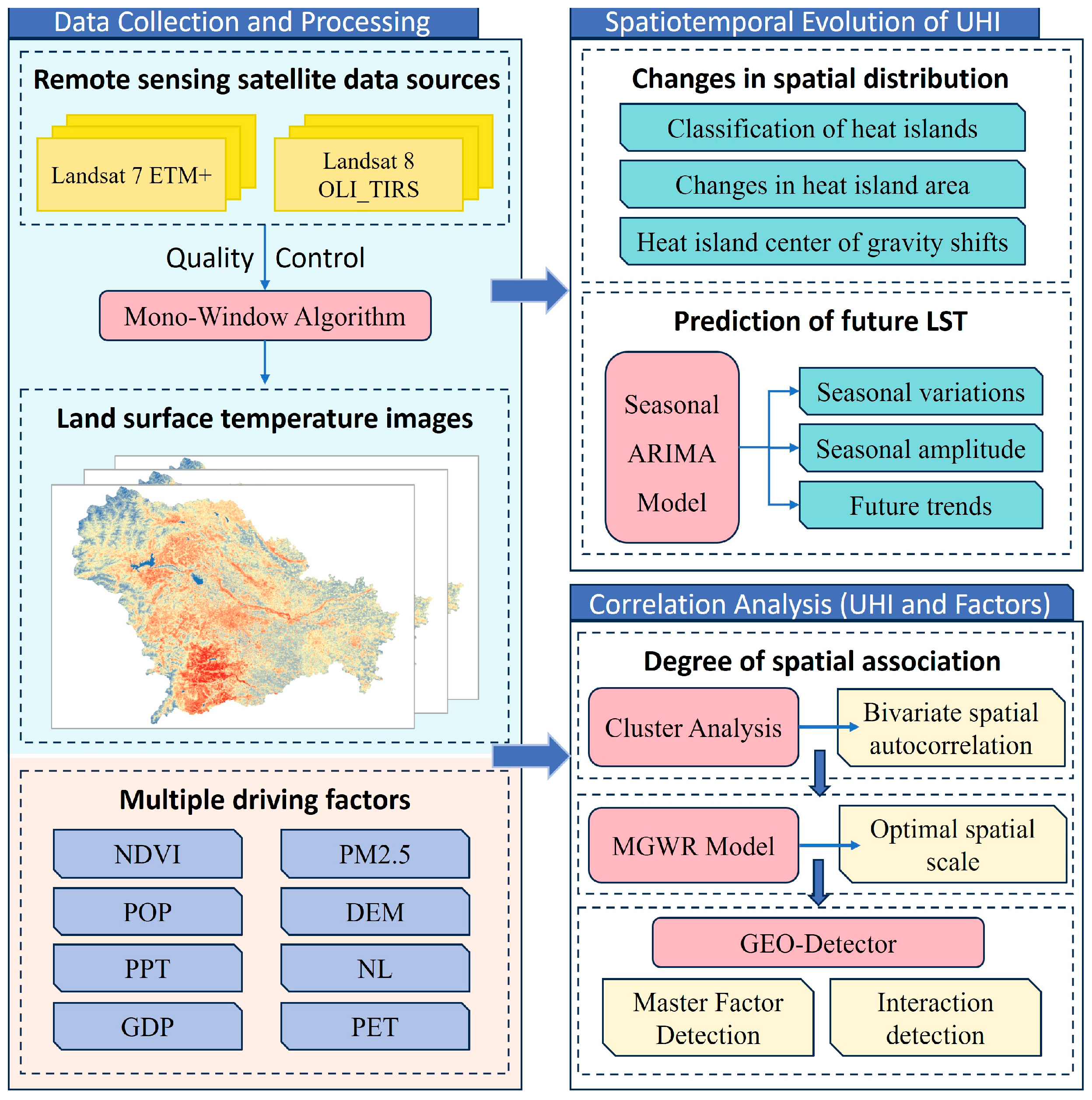
This study primarily employed remote sensing images from the Landsat7 ETM+ and Landsat8 OLI_TIRS series, which were sourced from the open-access EarthExplorer platform https://earthexplorer.usgs.gov (accessed on 4 May 2024). ETM+/OLI images were selected for their long-term temporal coverage and moderate spatial resolution, which balance the need for historical trend analysis and regional-scale pattern detection. The selected images were of sufficient quality for analysis. In processing the Landsat data, this study conducted essential radiometric and geometric corrections. During the LST retrieval phase, additional atmospheric correction was applied to the remote sensing data, enhancing retrieval accuracy and ensuring greater reliability of the results. The temporal and seasonal details of the remote sensing imagery used have been thoroughly summarized in Table 1.
In previous studies, the indices used to assess the influencing factors of UHIs have varied. The correlation between UHIs and these indices differs significantly due to variations in geographic location, climate conditions, and urban spatial structures, making it challenging to identify indices with consistent representativeness. Considering the findings from existing research and the characteristics of the city, several commonly used and easily quantifiable indices were selected, such as the NDVI (https://data.tpdc.ac.cn, accessed on 5 May 2024), PM2.5 (https://zenodo.org/record/6398971, accessed on 5 May 2024), NL (https://dataverse.harvard.edu, accessed on 5 May 2024), DEM (http://srtm.csi.cgiar.org/srtmdata, accessed on 5 May 2025), IPS (https://zenodo.org/records/5220816, accessed on 2 February 2025), PET (https://data.tpdc.ac.cn, accessed on 5 May 2024), POP (https://landscan.ornl.gov, accessed on 5 May 2024), and PPT (https://data.tpdc.ac.cn, accessed on 5 May 2024).

2.3. Methods

We employed the mono-window algorithm to retrieve surface temperature data and subsequently classified the results into distinct heat island categories. Utilizing the directional distribution method alongside the centroid model, we conducted a comprehensive analysis of the spatiotemporal distribution patterns of the UHI effect across various years and seasons. To predict future trends in UHI dynamics, the seasonal autoregressive integrated moving average (SARIMA) model was applied. Further, bivariate spatial autocorrelation analysis was employed to investigate the relationships between the UHI effect and its influencing factors over different time periods. Ultimately, a multi-scale spatial analysis model was developed, and the fitting accuracy of the geographically weighted regression model was assessed across different spatial scales. The geo-detector method was then used to analyze the contribution rates and interactions of various influencing factors, providing deeper insights into the mechanisms driving urban heat island formation. The specific process is shown in Figure 2.

2.3.1. LST Retrieval and Prediction

According to the characteristics of the Landsat data, the atmospheric correction method in the mono-window algorithm [30] is used to invert the LST. Under the premise of obtaining the average atmospheric operating temperature (T), surface specific emissivity (ε), and atmospheric transmittance (τ), the influence of atmospheric radiation on surface thermal radiation is estimated and eliminated, and the surface thermal radiation intensity is obtained, and then, the thermal radiation intensity is converted into the corresponding LST value.
The standard deviation ellipse is a commonly used tool in spatial statistical analysis to describe the shape and dispersion of data distributions [31]. By illustrating the distribution of LST data points, the standard deviation ellipse offers a visual representation of its spatial dispersion. The size of the ellipse reflects the extent to which data points are dispersed relative to the overall mean. The equation can be expressed as follows:
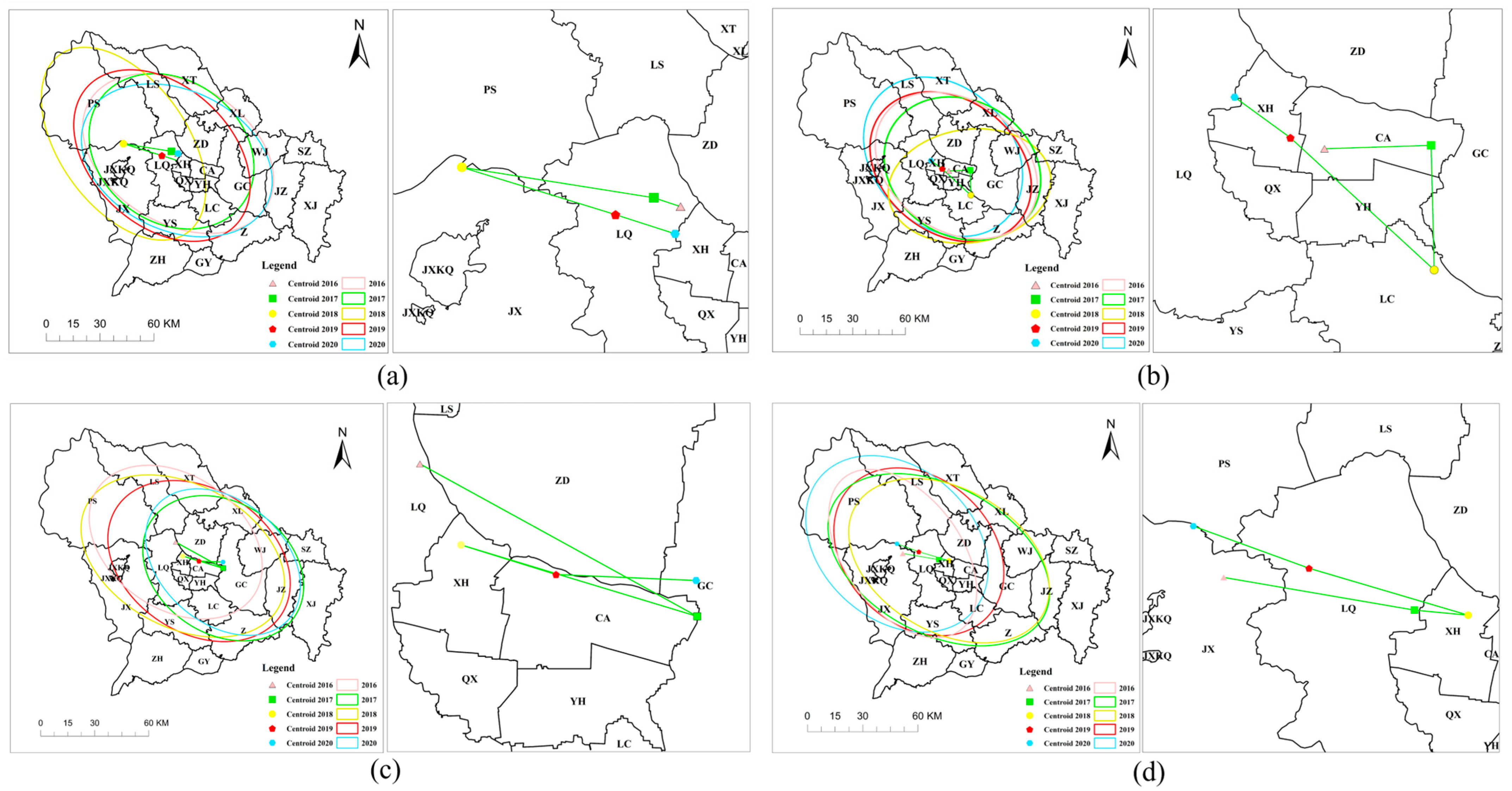
  • The center point of the ellipse:
X ¯ = i n ( x i x j ) 2 n ;   Y ¯ = i n ( y i y j ) 2 n
2.
The direction of the ellipse:
tan θ = A + B C
A = ( i = 1 n x ˜ t 2 i = 1 n y ˜ t 2 )
B = ( i = 1 n x ˜ t 2 i = 1 n y ˜ t 2 ) 2 + 4 ( i = 1 n x ˜ t y ˜ t ) 2
C = 2 i = 1 n x ˜ t y ˜ t
3.
The long and short semi-axes of the ellipse:
δ x = 2 i n ( x ˜ t cos θ y ˜ t sin θ ) 2 n ;   δ y = 2 i n ( x ˜ t sin θ y ˜ t cos θ ) 2 n
where x i and y i are the latitude and longitude coordinates of the data, x ¯ and y ¯ are the arithmetic mean center, x t and y t are the mean center, and x t ˜ and y t ˜ are the difference between the two coordinates.
The SARIMA model is a time series predicting method that extends the autoregressive integrated moving average (ARIMA) model [32,33] to account for seasonality. Implemented using the Box–Jenkins methodology for model identification, estimation, and prediction, the SARIMA model is particularly effective for real-time predictions and is known for its high accuracy. The SARIMA model introduces a seasonal component to capture seasonal changes in time series. Its mathematical representation is as follows:
SARIMA (p, d, q) (P, D, Q, s)
where p, d, and q represent the autoregressive order, the number of differences, and the moving average order, and P, D, Q, and s represent the seasonal autoregressive order, the seasonal number of differences, the seasonal moving average order, and the seasonal cycle.
The SARIMA model was chosen for this study due to its suitability for short- to medium-term predictions of time series data with seasonal patterns. Unlike long-term climate scenarios such as Shared Socioeconomic Pathways (SSPs), which rely on hypothetical socioeconomic projections and global climatic factors, SARIMA focuses purely on historical observational data. This approach enables fine-grained predictions at a local scale and aligns with this study’s emphasis on capturing periodic and short-term trends in UHI dynamics. The key advantages of SARIMA include the following: (1) Localized prediction: SARIMA effectively models city-scale temperature variations critical for understanding UHI effects. (2) Seasonality handling: The model’s seasonal components capture periodic LST fluctuations inherent to Landsat-derived data. (3) Simplicity and precision: SARIMA requires fewer assumptions than SSPs, prioritizing observed trends over speculative scenarios.

2.3.2. Spatial Autocorrelation Analysis

In this study, the global Moran’s I index [34] and its statistical test are used to analyze the spatial dependence characteristics of the data. The formula is as follows:
M o r a n s I = n i = 1 n j = 1 n ( x x ¯ ) ( x j x ¯ ) ( i = 1 n j = 1 n W i j ) j = 1 n ( x i x ¯ ) 2
where Moran’s I represents the global correlation index, n is the number of geographic units, W i j is the weight between geographic units i and j , x i and x j are the observed values of the geographic units i and j , and x ¯ is the average of all geographic unit observations.
Global spatial autocorrelation is a global index, which cannot reflect the local characteristics of the space, so the local spatial autocorrelation index proposed by Anselin in 1995 [35] was used to analyze the local spatial characteristics of the heat island area, and the calculation formula is as follows:
I i = ( x i x ¯ ) j n ( x j x ¯ ) 2 / n j = 1 , j i n W i j ( x j x ¯ )
where I i represents the local autocorrelation index, x i and x j represent the values of the related elements in the adjacent patches, and x ¯ is the average value. n is the total number of spatial patches; W i j is the adjacency weight; and m is the number of adjacencies.

2.3.3. Multi-Scale Spatial and Influencing Mechanism Analysis

In this study, the combination of the multi-scale geographically weighted regression model and the geo-detector model is referred to as the integrated geostatistical model.
Multi-scale geographically weighted regression (MGWR) [36] is an extension of local linear regression to model spatial variation relationships, which is based on the framework of geographically weighted regression (GWR) [37] and aims to more accurately characterize the complex relationships of spatial data. This model enables each geographic explanatory variable to have an independent scale of change, so as to better match the characteristics of spatial change. The formula for calculating the model is as follows:
y i = β 0 ( u i , v i ) + j = 1 k β b w j ( u i , v i ) x i j + ε i
where y i is the observed value of the dependent variable at position i , β 0 u i , v i is the constant term at the spatial location point, β b w j u i , v i is the regression coefficient of the j th independent variable at the spatial position i fitted by a specific broadband b w j , x i j represents the observed value of the independent variable at i , and ε i is the random error.
The geo-detector model [38] is a statistical method for analyzing spatial stratified heterogeneity, which can detect the spatial explanatory power and interaction of independent variables with dependent variables, as well as the significant differences between the two. As a method of spatial differentiation analysis, geo-detector is generally used to detect the driving force of analytical variables and can effectively analyze whether the influencing factors have an impact on the spatial differentiation of variables. In this study, factor detection and interaction detection were used. They are calculated as follows:
q = 1 h = 1 L N σ h 2 N σ 2 = 1 S S W S S T
S S W = h = 2 L N h σ h 2 , S S T = N σ 2
where q is in the range of [0, 1], and the closer to 1 it is, the greater the explanatory power of the dependent variable. L is the hierarchical of the dependent or independent variables, and N h and N are the number of units in layer h and the whole area, respectively. σ h 2 and σ 2 are the variances in the dependent variable for layer h and the whole area, respectively. S S W and S S T are the intra-layer variance and region-wide total variance.

3. Results and Discussion

3.1. Spatial and Temporal Evolution Characteristics of UHI

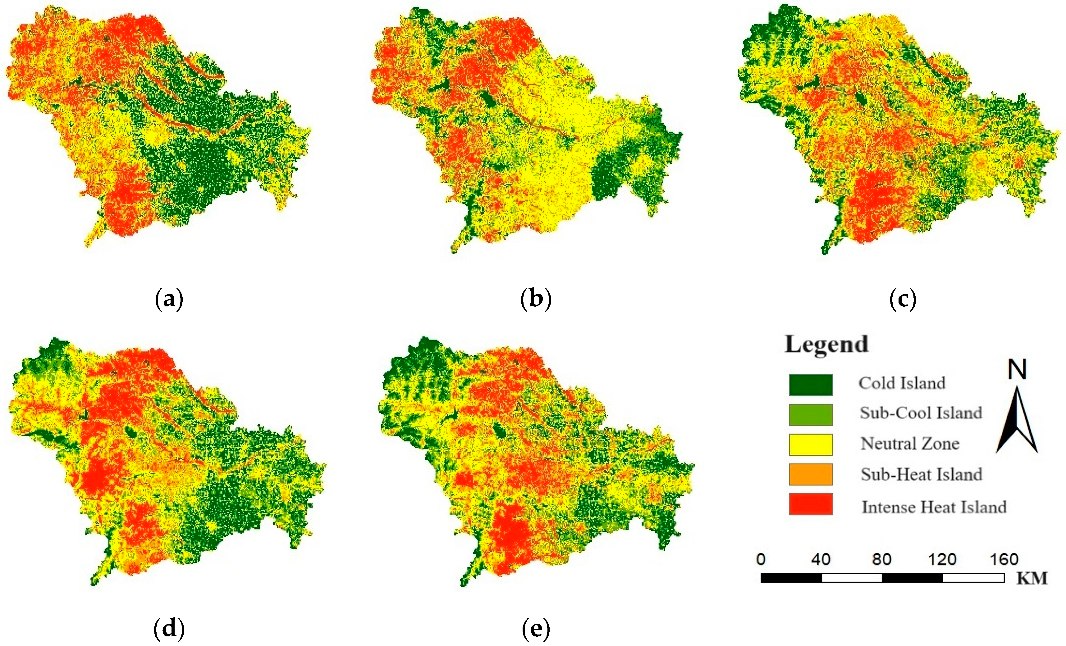
3.1.1. Classifications of UHI Pattern

At present, the equal-interval method and the mean–standard deviation method are widely used for classifying LST grades [39,40,41]. In this study, the mean–standard deviation method, which outperforms the equal-interval method in terms of sensitivity to UHI intensity classification and detailed representation [42], was selected. As shown in Table 2, the surface heat field is divided into five levels using the mean–standard deviation method. The high-temperature and sub-high-temperature areas are collectively referred to as the UHI areas according to the classifications. As shown in Figure 3, the heat island area in Shijiazhuang in 2000 covered 4577.56 km2, mainly concentrated in the western region, with strong heat island phenomena in the northwest and southwest. By 2005, the heat island areas remained concentrated in the northwest and southwest, but the southwest area decreased by 854.40 km2. In 2010, the heat island effect in the northwest eased and began to spread toward the central urban area, with the overall heat island area continuing to decrease by 753.85 km2. In 2015, the heat island area further reduced by 90.93 km2. By 2020, the heat island in the city center had expanded significantly, with an overall increase of 44.29 km2.
The distribution of the urban heat island effect in Shijiazhuang from 2016 to 2020 across the four seasons is shown in Figure 4. In the spring, the heat island areas were mainly located in the city center and its surrounding areas, forming a north–south corridor, with a notable exception in 2018 when the heat island areas were primarily in the western region. Overall, from 2016 to 2020, the spring heat island area gradually shrank from 4616.16 km2 to 4569.25 km2, reflecting an increase in non-heat island areas, which has a positive impact on improving the living environment.
The summer heat island areas from 2016 to 2020 expanded compared to the spring, mainly concentrated in the urban area along a north–south axis. In 2017, the heat island expanded eastward, but by 2019, it had shifted back to the central area, with a significant cold island phenomenon emerging in the northwest. The heat island area decreased from 4794.78 km2 to 4466.65 km2, showing an overall downward trend. This reflects Shijiazhuang’s efforts in greening and environmental optimization, effectively controlling the development of the heat island effect, which positively contributes to maintaining the quality of the living environment.
During the autumn from 2016 to 2020, the heat island areas were primarily concentrated in the central and eastern parts of Shijiazhuang. In 2018, the distribution of the urban heat island became more scattered. Overall, the heat island area significantly decreased from 4401.12 km2 to 4001.98 km2. The area of the normal zone reached its highest level, increasing to 6036.96 km2. Effective urban planning and ecological protection measures have somewhat mitigated the autumn heat island effect.
In the winter, from 2016 to 2020, the heat island areas were mostly concentrated in the central and western regions, with the exception of 2017 when the heat island was mainly in the central and eastern regions. Overall, the heat island area also decreased from 4145.33 km2 to 3995.15 km2. However, the heat island areas became more concentrated, particularly in the northwest, where the heat island situation was relatively severe.

3.1.2. Seasonal Variation in Spatial Pattern of UHI

The standard ellipses of the UHI in Shijiazhuang from 2016 to 2020 across different seasons provide a clear picture of its spatial distribution and temporal shifts (Figure 5).
Spring: The UHI generally followed a “northwest–southeast” distribution pattern. By 2020, the centroid had moved 3.87 km southward compared to 2016, with a noticeable trend of shifting westward initially, followed by a slight eastward movement. The centroid remained largely within Luquan District, except in 2018.
Summer: In 2018, the UHI’s spatial distribution showed a “southwest–northeast” orientation, but in other years, the “northwest–southeast” pattern was predominant. Over these years, the centroid shifted 11.8 km northwestward. The centroid exhibited considerable fluctuations, moving from Chang’an District to Luan District and then further northwest to Luquan District. Since 2018, the UHI’s center has consistently moved northwest, suggesting a potential future shift deeper into Luquan District.
Autumn: The UHI typically followed a “northwest–southeast” distribution trend. The centroid experienced significant displacement, shifting 28.51 km southeastward over five years. It moved from Luquan District to Chang’an District, then to Xinhua District, and eventually reached Gaocheng District.
Winter: The spatial distribution of the UHI in the winter generally exhibited a “southeast–northwest” pattern. Between 2016 and 2020, the centroid shifted 6.14 km northwestward. Since 2018, the UHI centroid has consistently moved in a northwest direction, indicating a potential continuation of this trend in the coming years.

3.2. Prediction of Future LST

For the 60 temperature values from 2016 to 2020, the data were arranged by year and season, prioritizing the lowest, average, and highest values for each season. A stationarity test and differencing were applied to the original sequence to ensure it met the requirements for time series modeling. Using the statsmodels.api package in Python 3.8, the optimal differencing parameters were identified to be (1, 1, 1) (1, 1, 0, 12) through grid search.
By analyzing the scatter plot of the predicted versus actual temperature values as shown in Figure 6a, several trends become evident. The actual temperature values over the validation period show a consistent pattern, with most of the predicted points aligning closely along the ideal fit line. However, there are some discrepancies, particularly at the extremes (i.e., higher temperatures), where the predicted values deviate from the ideal line. This suggests that while the model is highly accurate for moderate temperature ranges, it struggles to fully capture the dynamics of more extreme temperature values. The validation metrics reinforce these observations: an RMSE of 5.49 suggests a moderate level of error in the predictions, while an R2 of 0.91 demonstrates that the model explains 91% of the variance in the actual data, reflecting a high level of predictive accuracy. Additionally, the MAE of 4.91 further supports that the average prediction error is small, confirming the model’s overall robustness.
By visualizing the original sequence and predicted values of the seasonal LST in Shijiazhuang for the same period, as illustrated in Figure 6b, several trends emerge: In the original sequence of the seasonal LST, the seasonal LST in 2017, 2018, and 2020 remained relatively stable, fluctuating around a constant value, indicating a relatively stable seasonal pattern. However, the seasonal LST in 2016 and 2019 showed larger fluctuations, reflecting more pronounced seasonal changes. In the prediction sequence, the LST in Shijiazhuang from 2021 to 2027 is expected to show a slight upward trend, with regular cyclical fluctuations on a seasonal basis. The LSTs corresponding to different seasons are closely related, showing minor changes between seasons, while the LST fluctuations within each year across the four seasons are more significant.

3.3. Attribution Analysis of UHI

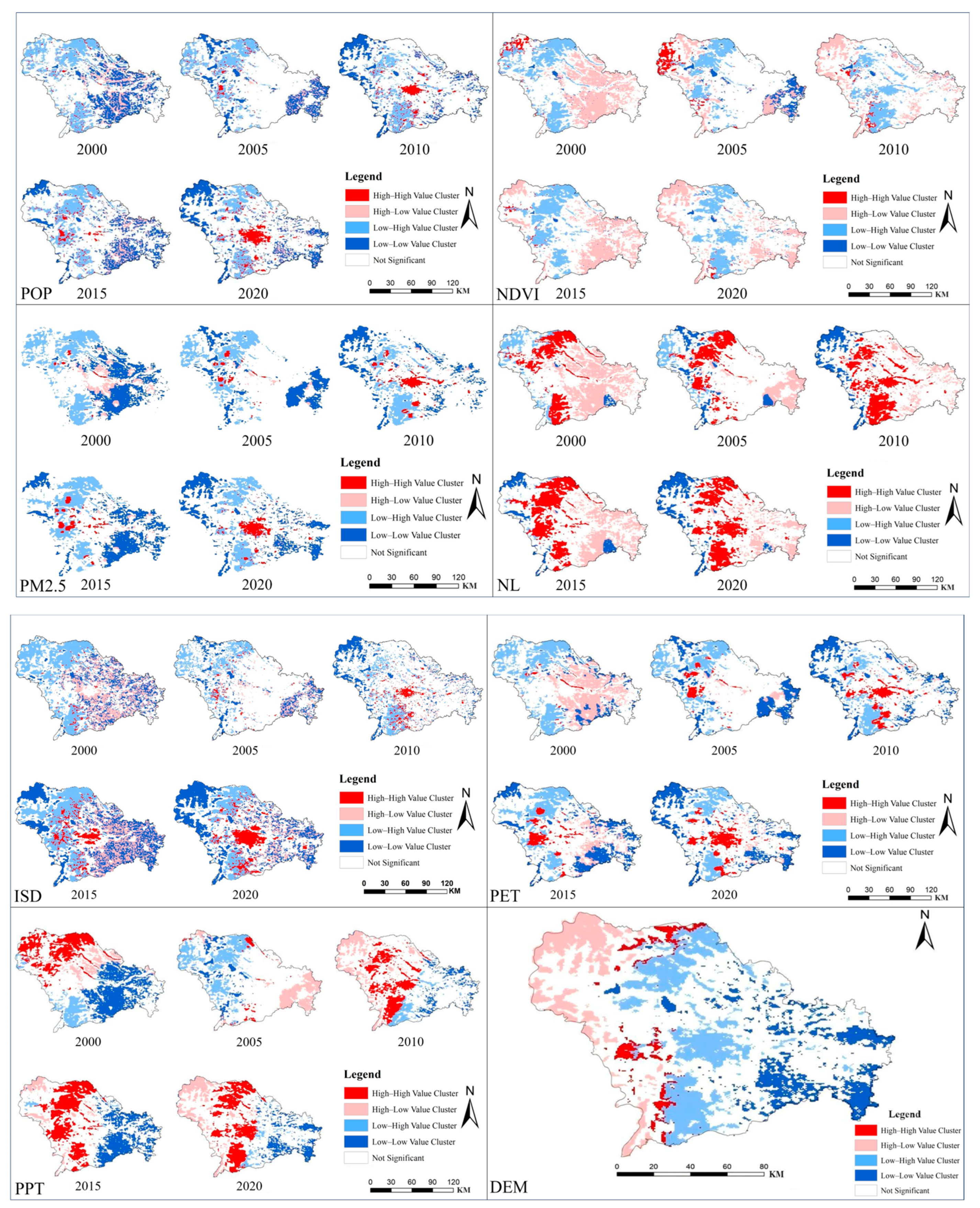
3.3.1. Analysis of Bivariate UHI Spatial Clustering Patterns

The bivariate spatial autocorrelation LISA cluster map is an effective tool for visualizing the spatial relationships between two variables. To investigate the spatial clustering and differentiation between urban heat islands and their influencing factors, a local autocorrelation analysis was conducted, which revealed the clustering patterns of urban heat islands in relation to various factors (as illustrated in Figure 7).
POP: In 2000, the population density and UHI showed little clustering, indicating a weak spatial relationship. By 2010, high-density urban areas saw an increase in the UHI effect, forming high–high positive clusters in the city center, while peripheral areas exhibited low–low clusters, where urbanization and the heat island effect were milder.
NDVI: Throughout 2000–2020, the NDVI showed a strong negative correlation with the UHI, signifying that increased vegetation mitigates UHI effects. This contrast became spatially pronounced over time, with central urban areas experiencing an intense UHI, highlighting the role of vegetation cover in mitigating heat effects.
IPS: Before 2005, the central urban areas of Shijiazhuang showed no significant spatial autocorrelation. However, from 2010 onward, the central urban areas began to exhibit pronounced “high–high” clusters, with both clustering and area reaching their peak by 2020. This marked the emergence of a more significant relationship between high impervious surface areas and elevated surface temperatures in the city’s core. In parallel, the “low–low” clusters in peripheral regions also expanded, highlighting a growing disparity between urban and rural areas in terms of temperature extremes.
PET: The spatial clustering pattern of PET is similar to that of the IPS, with the positive correlation in the central urban areas strengthening over time, though not as typical as in the IPS. Both reached their peak in 2020. Increased temperatures and urbanization likely accelerated atmospheric evapotranspiration, further intensifying the UHI.
PM2.5: High PM2.5 concentrations aligned with stronger UHI effects, especially in central areas, while regions with lower PM2.5 levels experienced a weaker UHI. This association underscores the link between air quality and the UHI and emphasizes the importance of managing pollution in urban planning.
NL: A positive correlation between NL and the UHI highlights that highly urbanized, brightly lit areas experience stronger UHI effects. Expanding clusters in the city center reflect an intensifying UHI alongside urban growth and socioeconomic development.
PPT: Aside from 2005, a positive correlation persisted between precipitation and the UHI, suggesting that higher rainfall contributes to UHI intensification. Increased red clusters (indicating high precipitation and UHI) in urban areas highlight how rainfall interacts with UHI dynamics.
DEM: Higher elevations were linked to weaker UHI effects, while lower, flat urban terrain corresponded to stronger UHI effects. This spatial differentiation, with mountainous areas exhibiting less UHI effects, indicates how terrain influences UHI distribution.
By analyzing these factors, it becomes evident that as the city continues to develop, the clustering patterns in the urban core have become more pronounced, and the heat island index in the city center is closely related to various influencing factors.

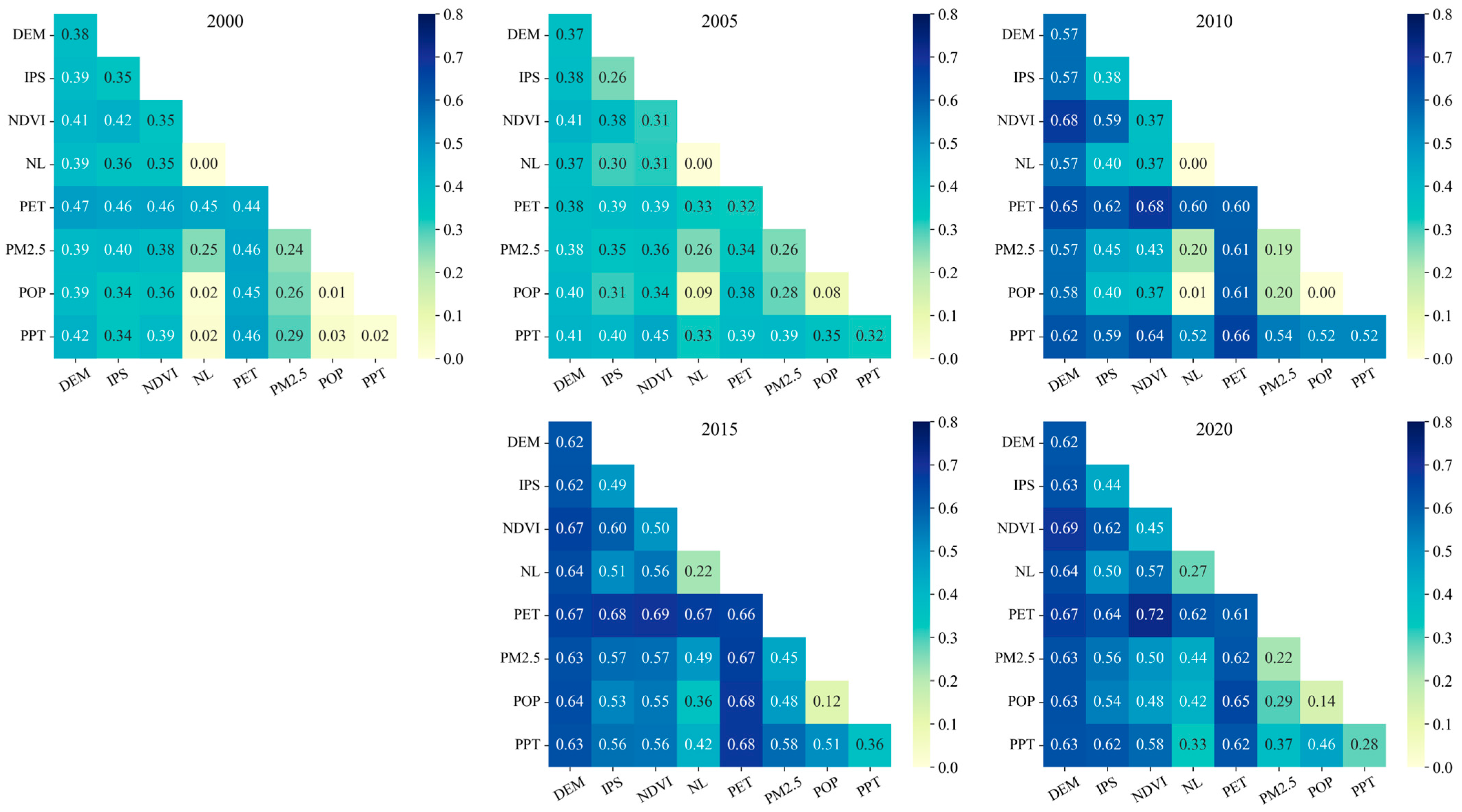
3.3.2. Analysis of Driving Factors Influencing UHI

To better understand how various spatial factors influence the intensity of the UHI at the neighborhood level and explore the interactions between these factors, this study utilizes the MGWR model and the geo-detector model.
The MGWR model’s goodness of fit is represented by the coefficient of determination R2. This study conducts calculations at five spatial scales. Analyzing the normalized values of the SHUI index for Shijiazhuang as spatial variables, the MGWR model results across different scales revealed that the R2 values are as follows: R 3   km 2 (0.645) > R 1   km 2 (0.644) > R 1.5   km 2 (0.637) > R 2   km 2 (0.632) > R 2.5   km 2 (0.581). This indicates that the model fits best at the 3 km grid scale for Shijiazhuang. Using this result as a reference, we performed geo-detector statistical analysis on each factor at the 3 km scale.
The geo-detector model allows for the analysis of key influencing factors and their interactions. In this research, the UHI data from Shijiazhuang serve as the dependent variable (Y), with various influencing factors as the independent variables (X). The goal was to examine the contribution of each factor to the UHI index and explore the interactions among them. Using the factor detector analysis, we determined the impact of these eight factors on the UHI intensity in Shijiazhuang. The results are summarized in Figure 8.
In all five phases of this study, the PET and DEM consistently exerted a significant influence on the UHI. After 2010, the q-values for both surpassed 0.5, with the peak value reaching 0.661 for PET. The influence of the NDVI and IPS followed, with their curves being closely aligned, though the q-value for the IPS in 2005 was below 0.3. The NDVI, PET, and DEM, all of which are closely linked to vegetation cover and evapotranspiration—two factors directly related to water availability—showed the strongest influence on the UHI. In the western region of Shijiazhuang, where the Taihang Mountains are located, the terrain’s high elevation results in lower vegetation cover, with large areas consisting of bare, rocky hills. This region exhibits higher UHI effects during the summer months, which explains why DEM’s influence is especially strong in this area. The PPT displayed a marked fluctuation. It was particularly low in 2000, but after 2005, the PPT remained above 0.3, suggesting that years with more regular or typical rainfall patterns had a greater impact on the UHI, potentially helping to mitigate heat island effects in the city. The PM2.5 levels fluctuated around 0.3 with minimal variation. While this shows some impact on the UHI, they remained less significant compared to other factors. In contrast, indicators such as nighttime light (NL) and population density (POP) had a much smaller influence on the UHI, generally remaining below 0.2. Notably, the influence of NL increased slightly after 2015, likely reflecting the growing intensity of human activities and urbanization.
Overall, the PET and DEM had the strongest influence, followed by the NDVI and IPS. In contrast, economic and demographic factors exhibited minimal impact, suggesting that human activities, while significant, may not be fully captured by the variables used in this analysis.
The interaction detector was applied to examine the extent to which two factors jointly affect UHI changes, with detailed results presented in Figure 9. The findings indicate that the combined effect of any two factors on the UHI intensity is significantly greater than that of individual factors.
The interactions among the PET, DEM, and NDVI exhibited strong synergy, with q-values exceeding 0.65 in years of high influence. The combination of the PET and NDVI peaked at 0.72 in 2020. The IPS also demonstrated a similarly close interaction with the previous three factors, with q-values reaching high levels as well. The PPT displayed fluctuating interaction effects with other factors. For example, its synergy with the NDVI and PET became more pronounced after 2005, with q-values rising above 0.6. Air quality, represented by PM2.5, showed modest interaction effects with natural factors. Its combined influence with the PET, for instance, remained stable at around 0.4 to 0.5 throughout the years. Factors such as the POP and NL individually had lower q-values (below 0.2 in most cases). However, their interactions with environmental variables like the NDVI and PET resulted in slightly elevated q-values, reaching up to 0.45 in 2020. This indicates that while single factors have a limited direct effect on UHI, the indirect effect of multiple factors through interactions cannot be ignored.
Notably, as time progressed, the synergistic effects between various factors grew stronger, indicating an increasing trend of collaborative influence on the UHI. This evolution highlights the importance of considering multifactor interactions in understanding and mitigating urban heat.

4. Discussion and Conclusions

4.1. Discussion

While SSPs are better suited for policy-driven, long-term climate projections at broader scales, SARIMA’s adaptability to localized datasets offers practical advantages for regional LST analysis. These methods are complementary and could be integrated in future studies to combine SARIMA’s precision with SSPs’ long-term insights.
The heat island classification method used in this study was adapted from Chen et al. [42], who originally applied it to a relatively small urban area (Fuzhou, less than 20 km in scale). While this approach worked well for Fuzhou, its application to the larger, more complex urban environment of Shijiazhuang may face certain challenges. In Figure 3 and Figure 4, the lack of a clear temperature contrast between Shijiazhuang’s urban center and its surrounding areas may reflect these challenges, indicating that the urban influence on temperature variations could be underestimated with the current classification approach. In future studies, we will explore alternative methods or adaptations to better capture large-scale UHI features.
Based on the results of MGWR and the geo-detector model, this study identifies the IPS and NDVI as key drivers of UHI intensity in Shijiazhuang. To mitigate UHI effects, urban planning strategies should prioritize reducing impervious surfaces in core urban areas through permeable pavement technologies and green infrastructure (e.g., rooftop gardens, urban parks). Additionally, expanding vegetation coverage, particularly in rapidly urbanizing zones, could mitigate UHI effects by enhancing evapotranspiration and shading. Optimizing urban spatial planning by balancing building density, road networks, and green spaces can further alleviate localized heat accumulation and improve ventilation corridors. Future policies in Shijiazhuang should consider mandating minimum green space ratios in new developments and incentivize retrofitting existing infrastructure with cooling materials. These measures could help reduce the intensity of the UHI and promote sustainable urban development.

4.2. Conclusions

This study provides a detailed and comprehensive analysis of the multi-scale methods used to examine the dynamic changes and influencing factors of the UHI. This research focuses on several key areas: the spatiotemporal dynamics of the UHI in Shijiazhuang from 2000 to 2020, seasonal time series prediction, the spatiotemporal correlation of influencing factors, multi-scale spatial analysis models, and integrated geostatistical approaches. The main findings are summarized as follows:
The urban heat island effect in Shijiazhuang exhibits distinct patterns and trends. From 2000 to 2020, the annual variation in the area of urban heat island zones decreased from 4577.56 km2 to 4430.53 km2, indicating a weakening of the urban heat island effect. Seasonal variations showed a decrease in the urban heat island area only in the autumn, from 4401.12 km2 in 2016 to 4001.98 km2 in 2020, while the areas in other seasons increased. The UHI in different seasons generally follows a southeast–northwest spatial direction. In the spring, the centroid shifted southward, while in the summer and winter, it moved northwestward. The most significant shift occurred in the autumn, with a southeastward movement of approximately 28 km.
The SARIMA model provided accurate predictions, with predictions falling within the 95% confidence interval. Overall, the LST in Shijiazhuang is projected to show a slight increasing trend from 2021 to 2027, with regular seasonal fluctuations, peaking in the summer of 2027.
The bivariate spatial autocorrelation results indicate that the NDVI was the most influential factor in mitigating the UHI, while the IPS spatially showed the most significant enhancement in the UHI in the central urban areas. Other factors generally promoted the UHI after 2005.
The contribution of influencing factors to the UHI is ranked as follows: PET > DEM > NDVI > IPS > PPT > PM2.5 > NL > POP. Among the factor interactions, the PET and NDVI have the most significant impact on the UHI, which can be as high as 0.72.

Author Contributions

Conceptualization, Y.L. and C.Z.; methodology, Y.L. and C.Z.; software, Y.L.; validation, X.Z. and G.S.; formal analysis, Y.L. and R.C.; investigation, Y.L. and R.C.; resources, C.Z. and R.C.; data curation, R.C.; writing—original draft preparation, Y.L. and R.C.; writing—review and editing, X.Z. and M.S.; visualization, Y.L., R.C., Y.T. and C.Z.; supervision, X.Z. and M.S.; project administration, X.Z. and G.S.; funding acquisition, X.Z. and M.S. All authors have read and agreed to the published version of the manuscript.

Funding

This research was funded by the Science Research Project of Hebei Education Department (QN2020212) and the National Natural Science Foundation of China (42201404).

Data Availability Statement

The data that support the findings of this study are openly available. The land surface temperature data from Landsat7 ETM+ and Landsat8 OLI_TIRS can be downloaded from https://earthexplorer.usgs.gov (accessed on 4 May 2024). The NDVI data are available at https://data.tpdc.ac.cn (accessed on 5 May 2024). The PM2.5 data are available at https://zenodo.org/record/6398971 (accessed on 5 May 2024). The NL data are available at https://dataverse.harvard.edu (accessed on 5 May 2024). The DEM data are from http://srtm.csi.cgiar.org/srtmdata/ (accessed on 5 May 2024). The IPS data are from https://zenodo.org/records/5220816 (accessed on 2 February 2025). The PET data are available at https://data.tpdc.ac.cn (accessed on 5 May 2024). The POP data are from https://landscan.ornl.gov/ (accessed on 5 May 2024) and PPT data available at https://data.tpdc.ac.cn (accessed on 5 May 2024).

Conflicts of Interest

The authors declare no conflicts of interest.

References

  1. Howard, L. The Climate of London: Deduced from Meteorological Observations Made in the Metropolis and at Various Places Around It; W. Phillips: London, UK, 1833. [Google Scholar]
  2. Oke, T.R. Boundary Layer Climates; Psychology Press: East Sussex, UK, 1987. [Google Scholar]
  3. Grimmond, S. Urbanization and global environmental change: Local effects of urban warming. Geogr. J. 2007, 173, 83–88. [Google Scholar] [CrossRef]
  4. Arnfield, A.J. Two decades of urban climate research: A review of turbulence, exchanges of energy and water, and the urban heat island. Int. J. Climatol. A J. R. Meteorol. Soc. 2003, 23, 1–26. [Google Scholar] [CrossRef]
  5. Oke, T.R.; Cleugh, H.A.; Grimmond, S.; Schmid, H.P.; Roth, M. Evaluation of spatially-averaged fluxes of heat, mass and momentum in the urban boundary layer. Weather. Clim. 1989, 9, 14–21. [Google Scholar] [CrossRef]
  6. Voogt, J.A.; Oke, T.R. Thermal remote sensing of urban climates. Remote Sens. Environ. 2003, 86, 370–384. [Google Scholar] [CrossRef]
  7. Rosenzweig, C.; Solecki, W.; Slosberg, R. Mitigating New York City’s Heat Island with Urban Forestry, Living Roofs, and Light Surfaces; New York State Energy Research and Development Authority: Albany, NY, USA, 2006; pp. 1–5. [Google Scholar]
  8. Wang, Z.; Liu, M.; Liu, X.; Meng, Y.; Zhu, L.; Rong, Y. Spatio-temporal evolution of surface urban heat islands in the Chang-Zhu-Tan urban agglomeration. Phys. Chem. Earth Parts A/B/C 2020, 117, 102865. [Google Scholar] [CrossRef]
  9. Deng, X.; Gao, F.; Liao, S.; Liu, Y.; Chen, W. Spatiotemporal evolution patterns of urban heat island and its relationship with urbanization in Guangdong-Hong Kong-Macao greater bay area of China from 2000 to 2020. Ecol. Indic. 2023, 146, 109817. [Google Scholar] [CrossRef]
  10. Min, M.; Zhao, H.; Miao, C. Spatio-temporal evolution analysis of the urban heat island: A case study of Zhengzhou City, China. Sustainability 2018, 10, 1992. [Google Scholar] [CrossRef]
  11. Sun, L.; Hang, X.; Gao, P.; Xie, X.; Zhu, S.; Li, Y. Characteristics of summer urban heat island in Jiangsu Province by multi-year satellite observations. J. Meteorol. Sci. 2023, 43, 662–669. [Google Scholar]
  12. Hu, N.; Ren, Z.; Dong, Y.; Fu, Y.; Guo, Y.; Mao, Z.; Chang, X. Spatio-temporal Evolution of Heat Island Effect and Its Driving Factors in Urban Agglomerations of China. Sci. Geogr. Sin. 2022, 42, 1534–1545. [Google Scholar] [CrossRef]
  13. Si, M.; Li, Z.L.; Nerry, F.; Tang, B.H.; Leng, P.; Wu, H.; Zhang, X.; Shang, G. Spatiotemporal pattern and long-term trend of global surface urban heat islands characterized by dynamic urban-extent method and MODIS data. ISPRS J. Photogramm. Remote Sens. 2022, 183, 321–335. [Google Scholar] [CrossRef]
  14. Zhang, Z.; Paschalis, A.; Mijic, A.; Meili, N.; Manoli, G.; van Reeuwijk, M.; Fatichi, S. A mechanistic assessment of urban heat island intensities and drivers across climates. Urban Clim. 2022, 44, 101215. [Google Scholar] [CrossRef]
  15. Khalil, U.; Aslam, B.; Azam, U.; Khalid, H.M.D. Time series analysis of land surface temperature and drivers of urban heat island effect based on remotely sensed data to develop a prediction model. Appl. Artif. Intell. 2021, 35, 1803–1828. [Google Scholar] [CrossRef]
  16. He, Z.; Zhang, D.; Ye, Q.; Chen, Z.; Yang, S.; Gao, Y. Characteristics of urban heat island in Chongqing in recent 40 years and its association with weather conditions. Arid. Meteorol. 2022, 40, 683–689. [Google Scholar] [CrossRef]
  17. Niu, L.; Zhang, Z.; Peng, Z.; Jiang, Y.; Liu, M.; Zhou, X.; Tang, R. China’s surface urban heat island drivers and its spatial heterogeneity. China Environ. Sci. 2022, 42, 945–953. [Google Scholar]
  18. Liao, Y.; Shen, X.; Zhou, J.; Ma, J.; Zhang, X.; Tang, W.; Chen, Y.; Ding, L.; Wang, Z. Surface urban heat island detected by all-weather satellite land surface temperature. Sci. Total Environ. 2022, 811, 151405. [Google Scholar] [CrossRef]
  19. Ma, J.; Zhou, J.; Zhang, T.; Tang, W.; Liao, Y.; Yang, M. Non-negligible clear-sky biases of satellite thermal infrared observations for analyzing surface urban heat island intensity: A case study in China. Sci. Total Environ. 2024, 949, 174928. [Google Scholar] [CrossRef] [PubMed]
  20. Deilami, K.; Kamruzzaman, M.; Liu, Y. Urban heat island effect: A systematic review of spatio-temporal factors, data, methods, and mitigation measures. Int. J. Appl. Earth Obs. Geoinf. 2018, 67, 30–42. [Google Scholar] [CrossRef]
  21. Almeida, C.R.; Teodoro, A.C.; Gonçalves, A. Study of the urban heat island (UHI) using remote sensing data/techniques: A systematic review. Environments 2021, 8, 105. [Google Scholar] [CrossRef]
  22. Mirzaei, P.A.; Haghighat, F. Approaches to study urban heat island–abilities and limitations. Build. Environ. 2010, 45, 2192–2201. [Google Scholar] [CrossRef]
  23. Rajasekar, U.; Weng, Q. Urban heat island monitoring and analysis using a non-parametric model: A case study of Indianapolis. ISPRS J. Photogramm. Remote Sens. 2009, 64, 86–96. [Google Scholar] [CrossRef]
  24. Jiménez-Muñoz, J.C.; Sobrino, J.A. A single-channel algorithm for land-surface temperature retrieval from ASTER data. IEEE Geosci. Remote Sens. Lett. 2009, 7, 176–179. [Google Scholar] [CrossRef]
  25. Li, H.; Liu, Q.; Zhong, B.; Du, Y.; Wang, H.; Wang, Q. A single-channel algorithm for land surface temperature retrieval from HJ-1B/IRS data based on a parametric model. In Proceedings of the 2010 IEEE International Geoscience and Remote Sensing Symposium, Honolulu, HI, USA, 25–30 July 2010; pp. 2448–2451. [Google Scholar]
  26. Price, J.C. Land surface temperature measurements from the split window channels of the NOAA 7 Advanced Very High Resolution Radiometer. J. Geophys. Res. Atmos. 1984, 89, 7231–7237. [Google Scholar] [CrossRef]
  27. Mao, K.; Qin, Z.; Shi, J.; Gong, P. The Research of Split-Window Algorithm on th e MODIS. Geomat. Inf. Sci. Wuhan Univ. 2005, 30, 703–707. [Google Scholar]
  28. Ulivieri, C.M.M.A.; Castronuovo, M.M.; Francioni, R.; Cardillo, A. A split window algorithm for estimating land surface temperature from satellites. Adv. Space Res. 1994, 14, 59–65. [Google Scholar] [CrossRef]
  29. Zheng, Z.; Xu, G.; Wang, Y.; Li, Q.; Li, J. Characteristics and Main Influence Factors of Heat Waves in Beijing–Tianjin–Shijiazhuang Cities of Northern China in Recent 50 Years. Atmos. Sci. Lett. 2020, 21, e1001. [Google Scholar] [CrossRef]
  30. Qin, Z.H.; Zhang, M.H.; Karnieli, A.; Berliner, P. Mono-window algorithm for retrieving land surface temperature from Landsat TM6 data. Acta Geogr. Sin. 2001, 56, 456–466. [Google Scholar]
  31. Yuill, R. Standard Deviational Ellipse—Updated Tool For Spatial Description. Geogr. Anal. 1971, B 53, 28–39. [Google Scholar] [CrossRef]
  32. Box GE, P.; Pierce, D.A. Distribution of residual autocorrelations in autoregressive-integrated moving average time series models. J. Am. Stat. Assoc. 1970, 65, 1509–1526. [Google Scholar] [CrossRef]
  33. Mathew, A.; Sreekumar, S.; Khandelwal, S.; Kaul, N.; Kumar, R. Prediction of land-surface temperatures of Jaipur city using linear time series model. IEEE J. Sel. Top. Appl. Earth Obs. Remote Sens. 2016, 9, 3546–3552. [Google Scholar] [CrossRef]
  34. Moran, P.A. Notes on Continuous Stochastic Phenomena. Biometrika 1950, 37, 17–23. [Google Scholar] [CrossRef] [PubMed]
  35. Anselin, L. Local Indicators of Spatial Association—Lisa. Geogr. Anal. 1995, 27, 93–115. [Google Scholar] [CrossRef]
  36. Fotheringham, A.S.; Yang, W.; Kang, W. Multiscale Geographically Weighted Regression (Mgwr). Ann. Am. Assoc. Geogr. 2017, 107, 1247–1265. [Google Scholar] [CrossRef]
  37. Brunsdon, C.; Fotheringham, A.S.; Charlton, M. Some Notes on Parametric Significance Tests for Geographically Weighted Regression. J. Reg. Sci. 1999, 39, 497–524. [Google Scholar] [CrossRef]
  38. Wang, J.; Xu, C. Geodetector: Principle and prospective. Acta Geogr. Sin. 2017, 72, 116–134. [Google Scholar] [CrossRef]
  39. Li, L.; Wang, H.; Jia, Q.; Lü, G.; Wang, X.; Zhang, Y.; Ai, J. Urban heat island intensity and its grading in Liaoning Province of Northeast China. Chin. J. Appl. Ecol. 2012, 23, 1345–1350. [Google Scholar]
  40. Zhang, Y.; Yu, T.; Gu, X.F.; Zhang, Y.X.; Chen, L.F. Land surface temperature retrieval from CBERS-02 IRMSS thermal infrared data and its applications in quantitative analysis of urban heat island effect. J. Remote Sens. 2006, 10, 789–797. [Google Scholar]
  41. Yu, C.; Hu, D.; Cao, S. Spatio-temporal pattern of heat island and multivariate modeling of impact factors of Beijing downtown from 2005 to 2016. J. Geo-Inf. Sci. 2017, 19, 1485–1494. [Google Scholar]
  42. Chen, S.; Wang, T. Comparison Analyses of Equal Interval Method and Mean-standard Deviation Method Used to Delimitate Urban Heat Island. J. Geo-Inf. Sci. 2009, 11, 145–150. [Google Scholar] [CrossRef]
Figure 1. Overview of the study area.
Remotesensing 17 00781 g001
Figure 2. Framework for the research process.
Remotesensing 17 00781 g002
Figure 3. Spatial distribution of UHI in Shijiazhuang. (a) 2000; (b) 2005; (c) 2010; (d) 2015; (e) 2020.
Remotesensing 17 00781 g003
Figure 4. Spatial distribution of UHI in Shijiazhuang for four seasons (2016–2020).
Remotesensing 17 00781 g004
Figure 5. UHI centroid shifts by season (2016–2020). (a) Spring; (b) summer; (c) autumn; (d) winter. PS: Pingshan County; LQ: Luquan District; ZH: Zanhuan County; QX: Qiaoxi District; SZ: Shenze County; GC: Gaocheng District; CA: Changan District; ZD: Zhengding County; JXKQ: Jingxing Ore District; XJ: Xingjing city; WJ: Wuji County; YH: Yuhua District; XT: Xingtang County; Z: Zhaoxian County; GY: Gaoyi County; YS: Yuanshi County; LC: Luanchen District; JZ: Jingzhou city; JX: Jingxing County; XH: Xinhua District; XL: Xingle city; LS: Lingshou County.
Remotesensing 17 00781 g005
Figure 6. (a) Scatter plot of predicted and actual values. (b) LST prediction for Shijiazhuang (unit: °C). Each vertex of the line represents one season.
Remotesensing 17 00781 g006
Figure 7. Cluster analysis of the key factors associated with the UHI index.
Remotesensing 17 00781 g007
Figure 8. Factor detector q-statistics results of single factor.
Remotesensing 17 00781 g008
Figure 9. Interaction detector Q-value heatmap.
Remotesensing 17 00781 g009
Table 1. Information on remote sensing image data.
Sensor TypesDateSpatial Resolution
Landsat7 ETM+23 May 2020 22 Jun. 2005 19 May 201030 m
Landsat8 OLI_TIRS25 May 2015 03 Dec. 2015 25 Apr. 2016
12 Jun. 2016 18 Oct. 2016 22 Jan. 2017
12 Apr. 2017 01 Jul. 2017 05 Oct. 2017
24 Dec. 2017 14 Mar. 2018 20 Jul. 2018
24 Oct. 2018 11 Dec. 2018 02 Apr. 2019
20 May 2019 13 Oct. 2019 31 Jan. 2020
19 Mar. 2020 22 May 2020 13 Oct. 2020
30 m
Table 2. LST heat rating scale.
Temperature Zone LevelsHeat Island LevelsTemperature Range
High-temperature zoneIntense heat islandT > u + std
Sub-high-temperature zoneSub-heat islandu + 0.5 std < T < u + std
Medium-temperature zoneNeutral zoneu − 0.5 std < T < u + 0.5 std
Sub-low-temperature zoneSub-cold islandustd < T < u − 0.5 std
Low-temperature zoneCold islandT < ustd
where T is temperature, u is mean temperature, and std is standard deviation.
Disclaimer/Publisher’s Note: The statements, opinions and data contained in all publications are solely those of the individual author(s) and contributor(s) and not of MDPI and/or the editor(s). MDPI and/or the editor(s) disclaim responsibility for any injury to people or property resulting from any ideas, methods, instructions or products referred to in the content.

