
A Novel Dual-Branch Pansharpening Network with High-Frequency Component Enhancement and Multi-Scale Skip Connection


Abstract

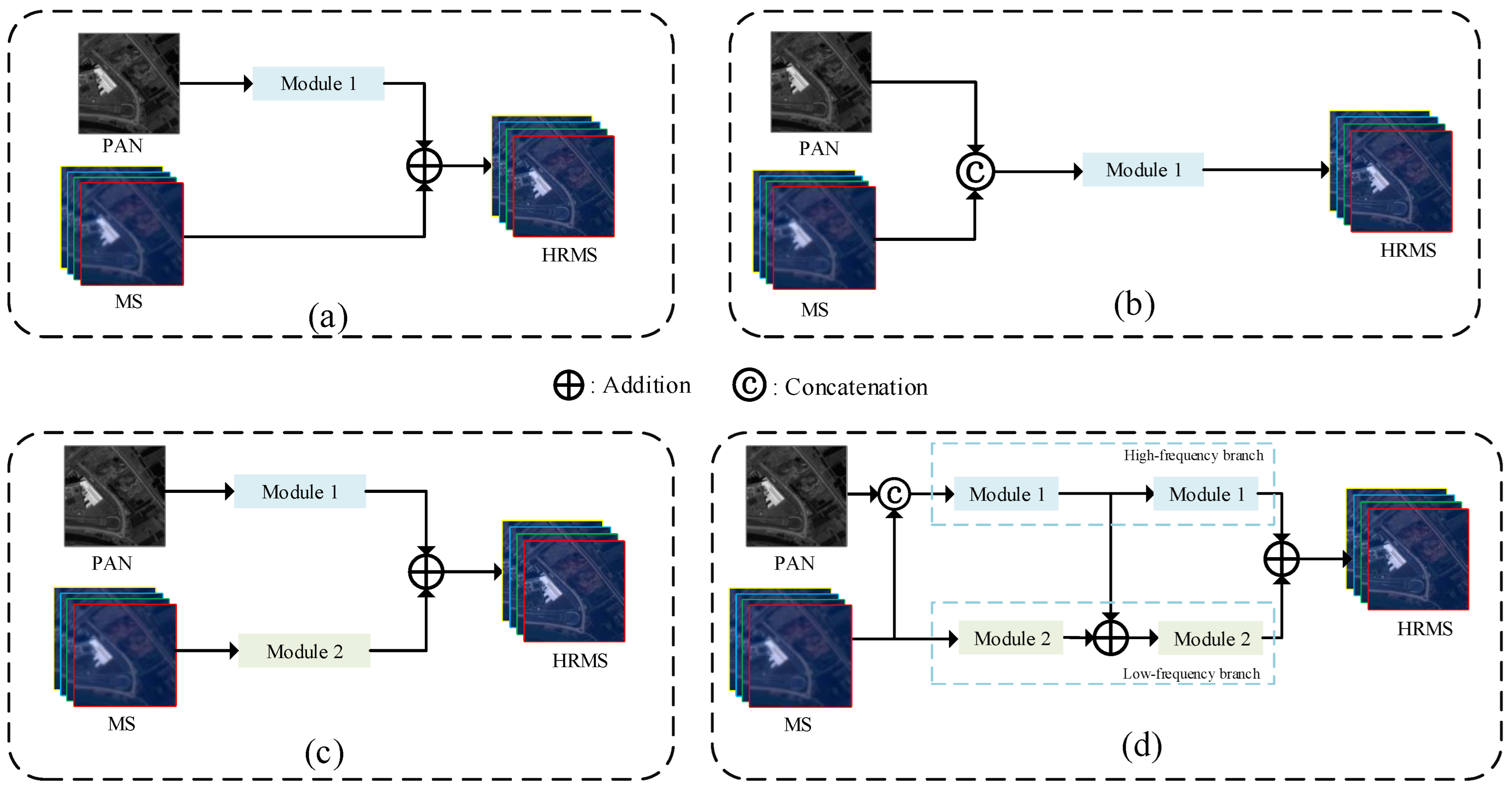
1. Introduction
- We propose a novel dual-branch fusion network. While fully extracting high- and low-frequency information, it solves the problem that traditional networks ignore the differences and correlations between PAN and MS images.
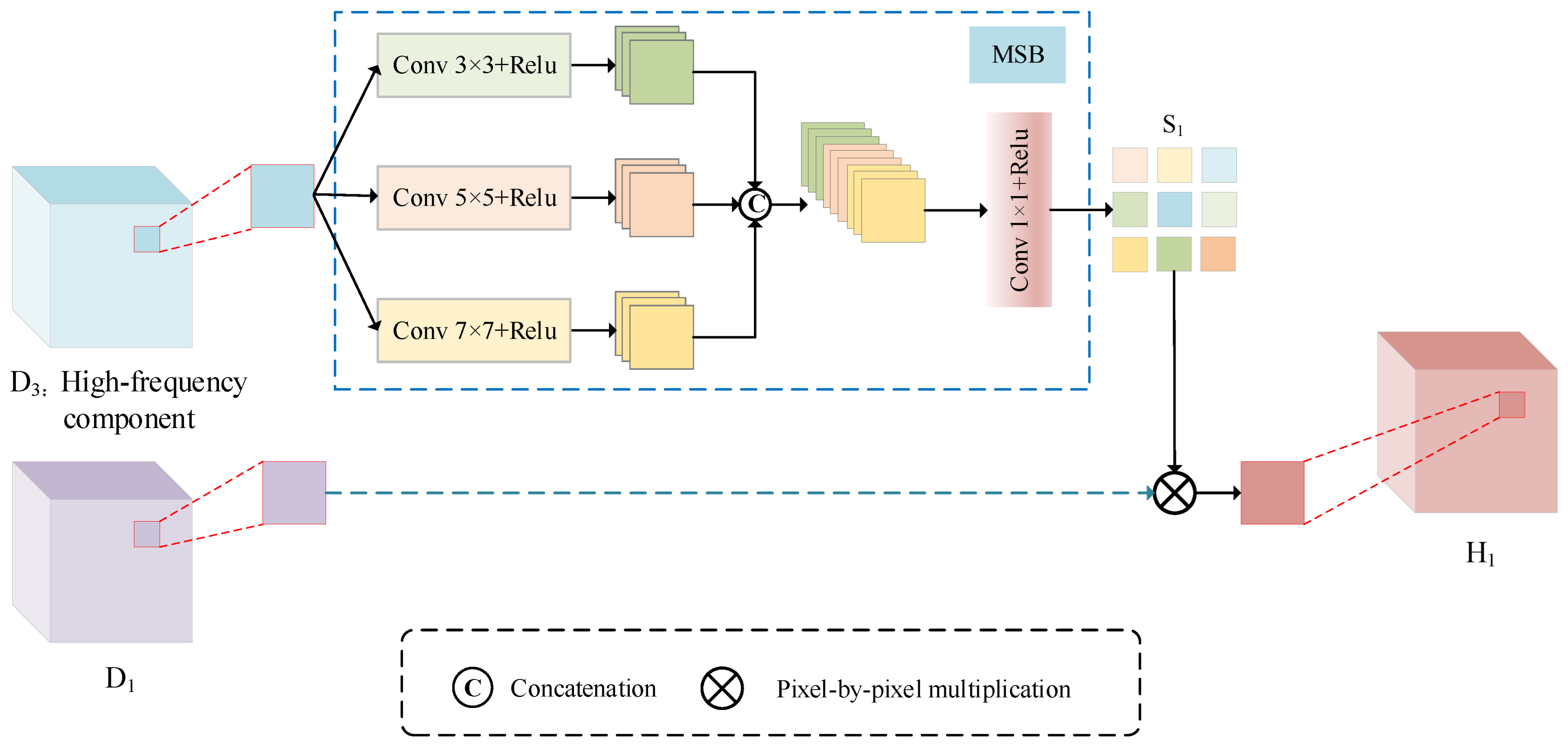
- In the high-frequency branch, we designed HFCEM. Multi-scale block (MSB) processing is performed on the extracted high-frequency component to generate weights and fully extract high-frequency information. The proposed HFCEM is able to effectively utilize the correlations between images and exhibits excellent performance in recovering texture details.
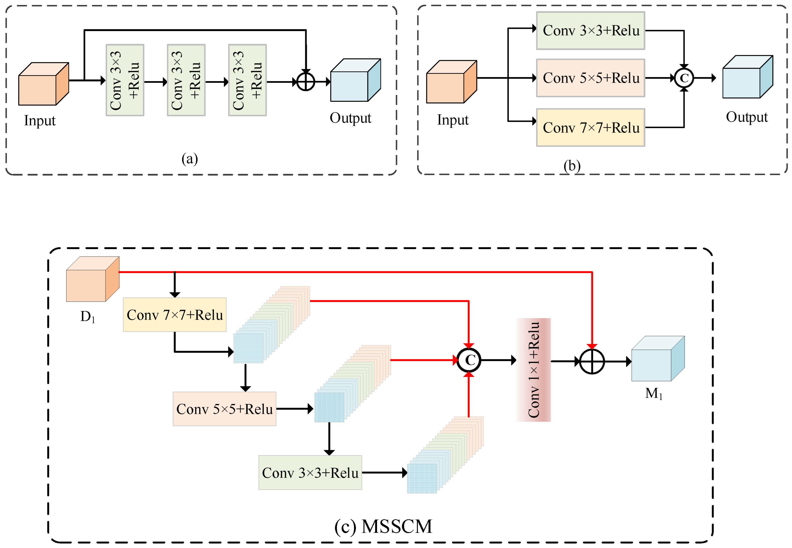
- In the low-frequency branch, we further designed MSSCM. This module is able to effectively capture features at different scales by combining multi-scale convolution and skip connections, and reuse shallow information features to better extract the overall contour information.
2. Related Work
3. Proposed Method
3.1. HFCEM
3.2. MSSCM
3.3. Loss Function
4. Experiments and Results
4.1. Experimental Design
4.2. Methods of Comparison
4.3. Evaluation Indicators
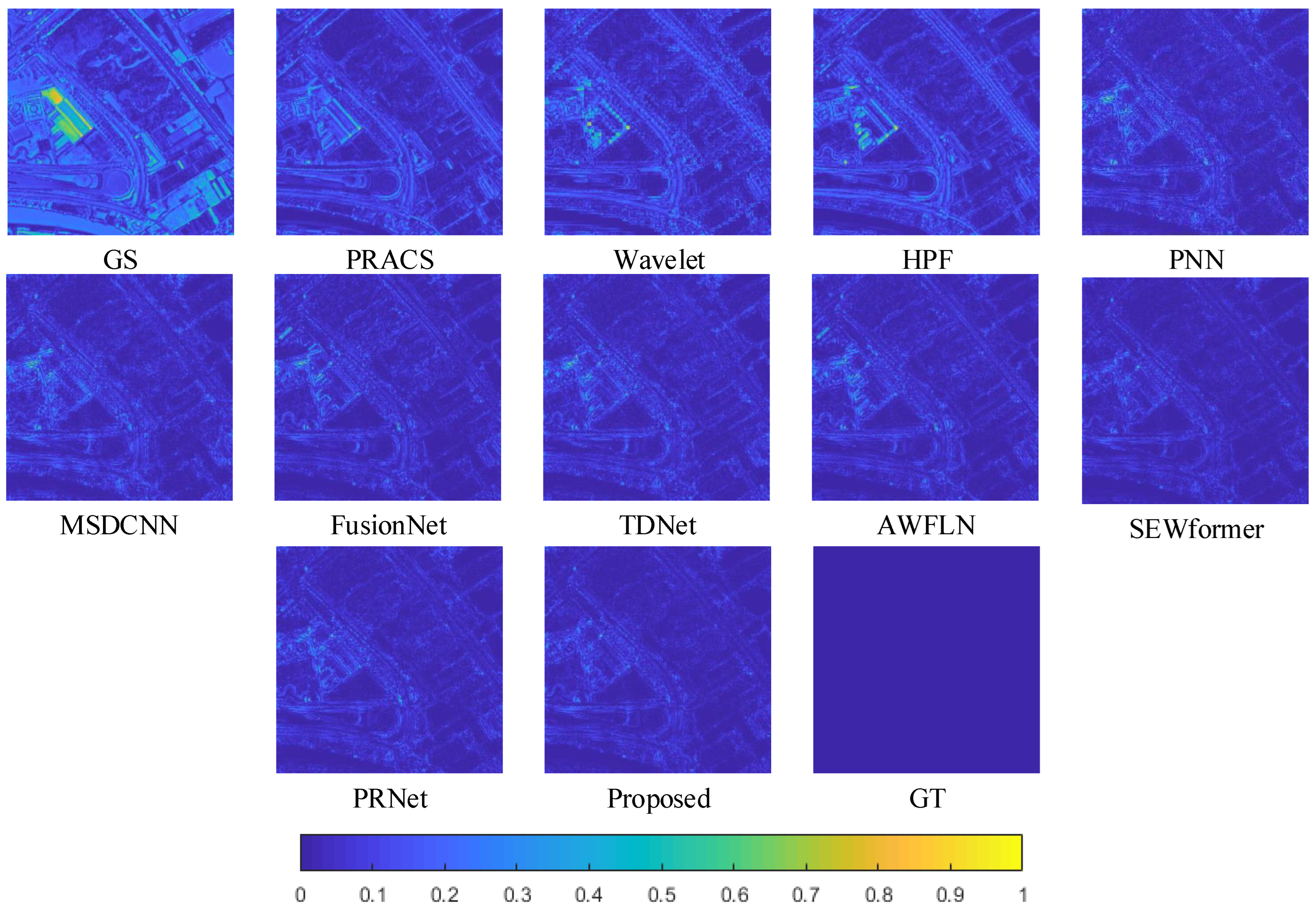
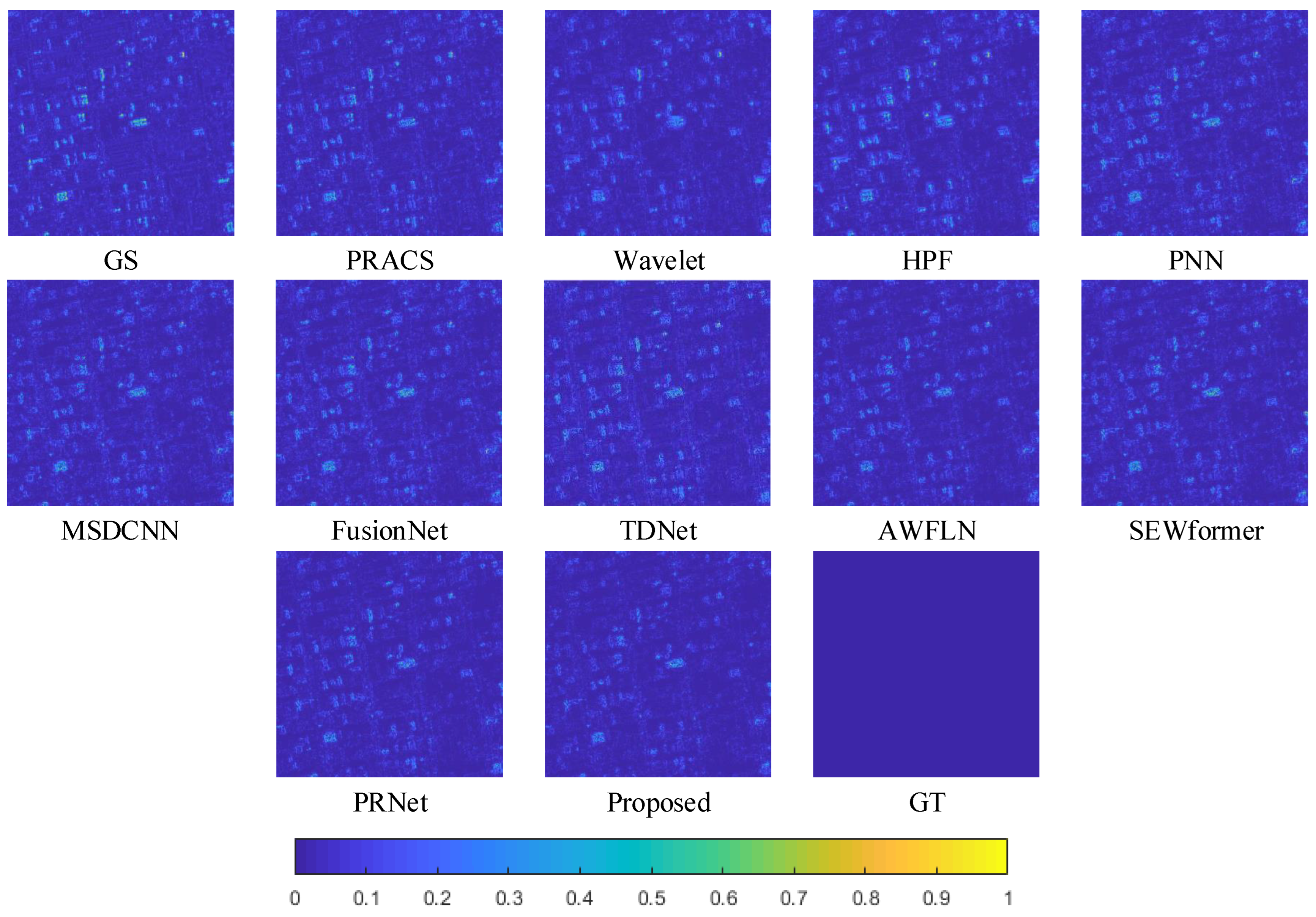
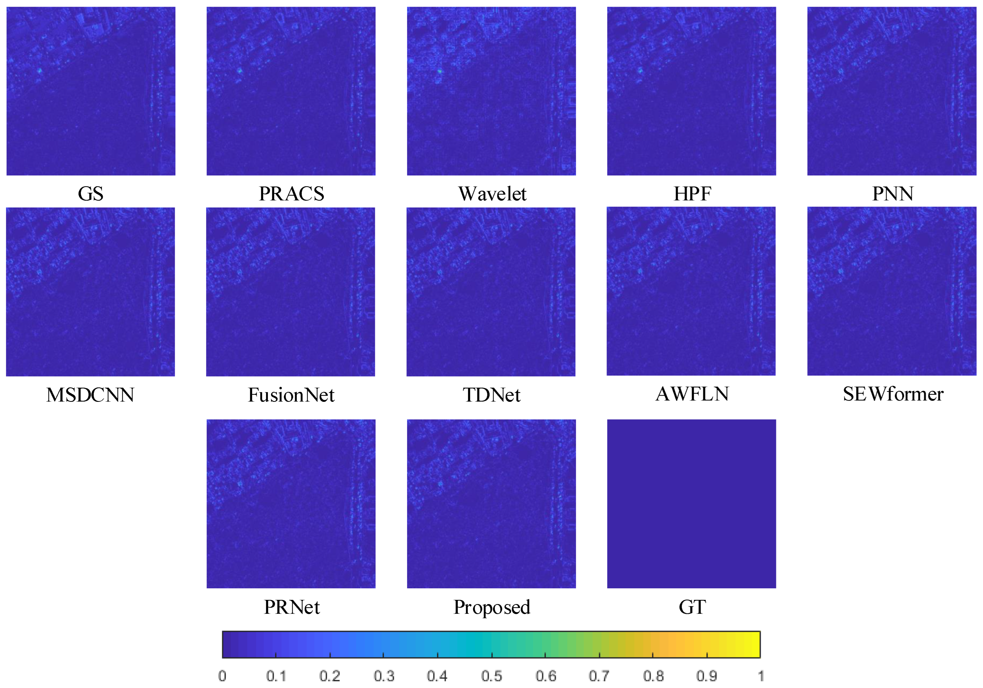
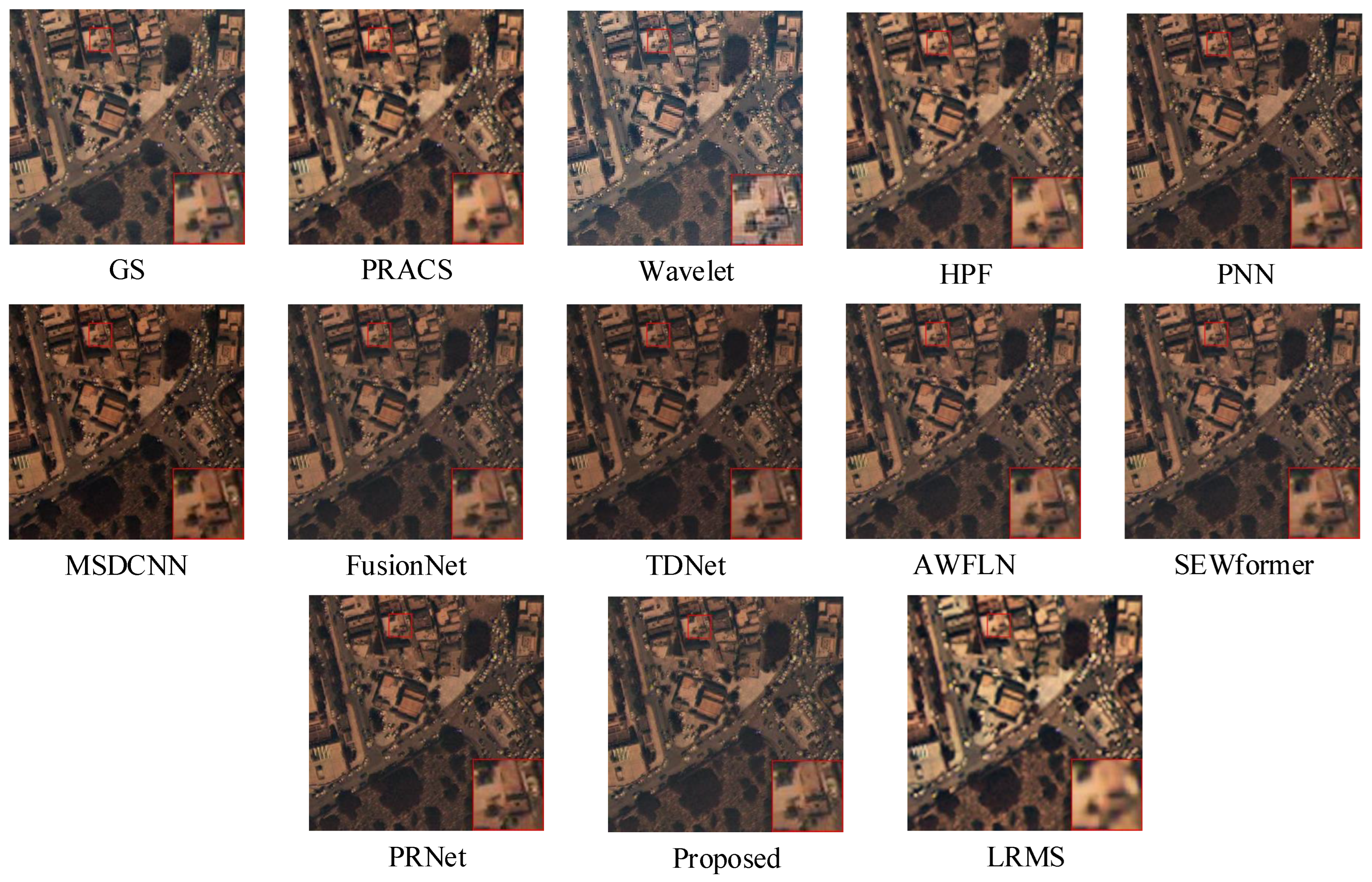
4.4. Reduced-Scale Experiments
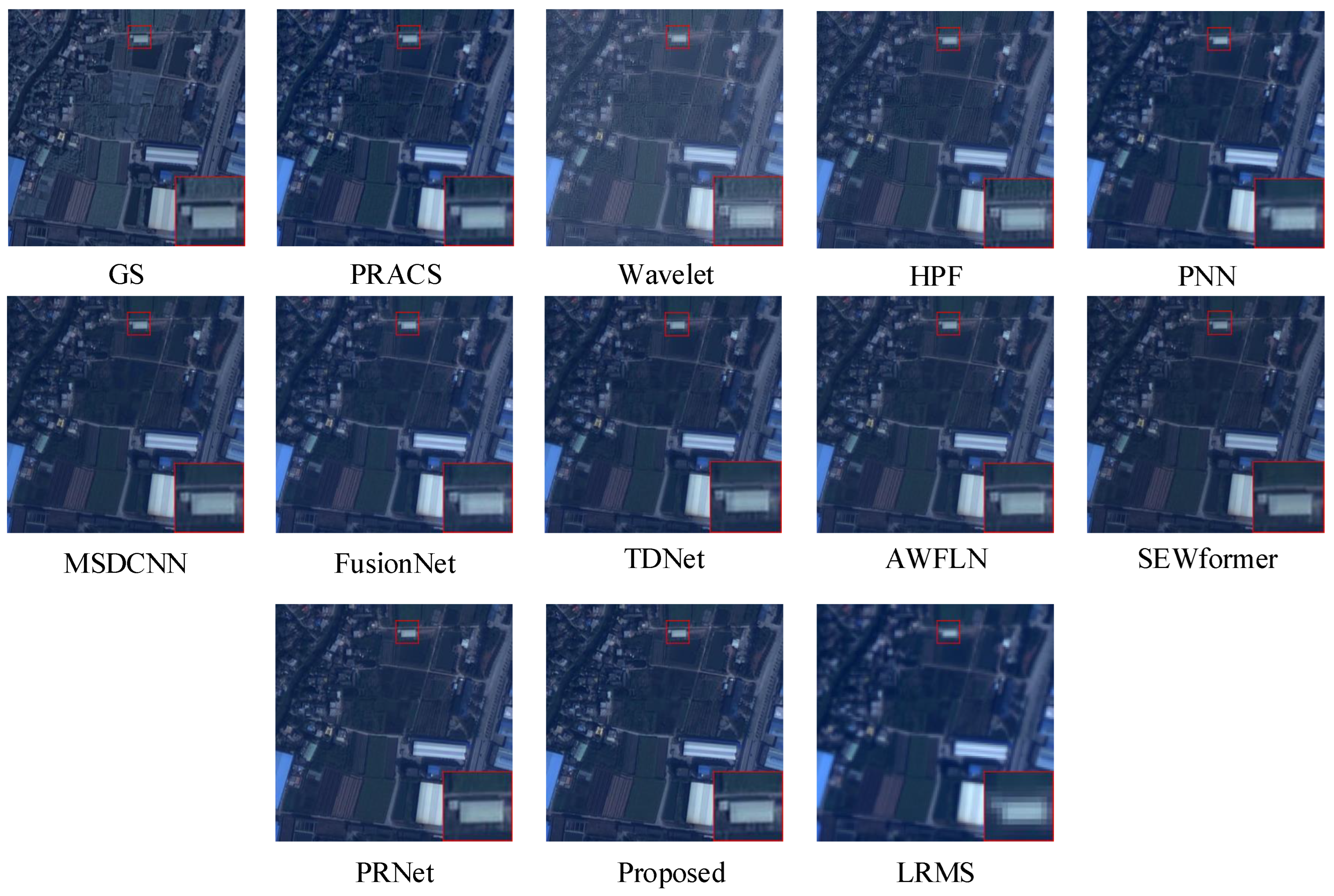
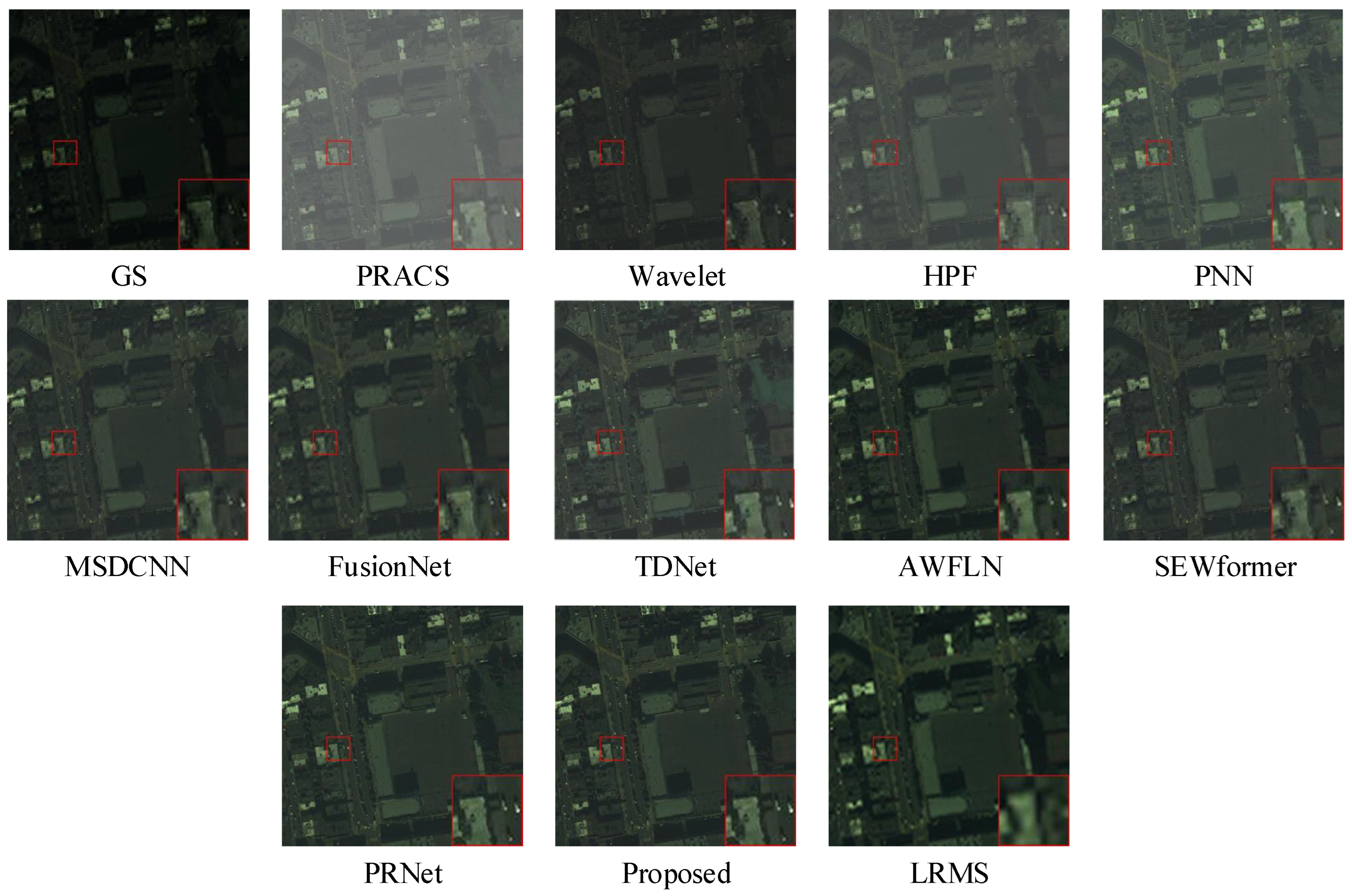
4.5. Full-Scale Experiments
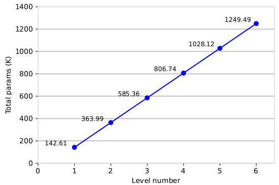
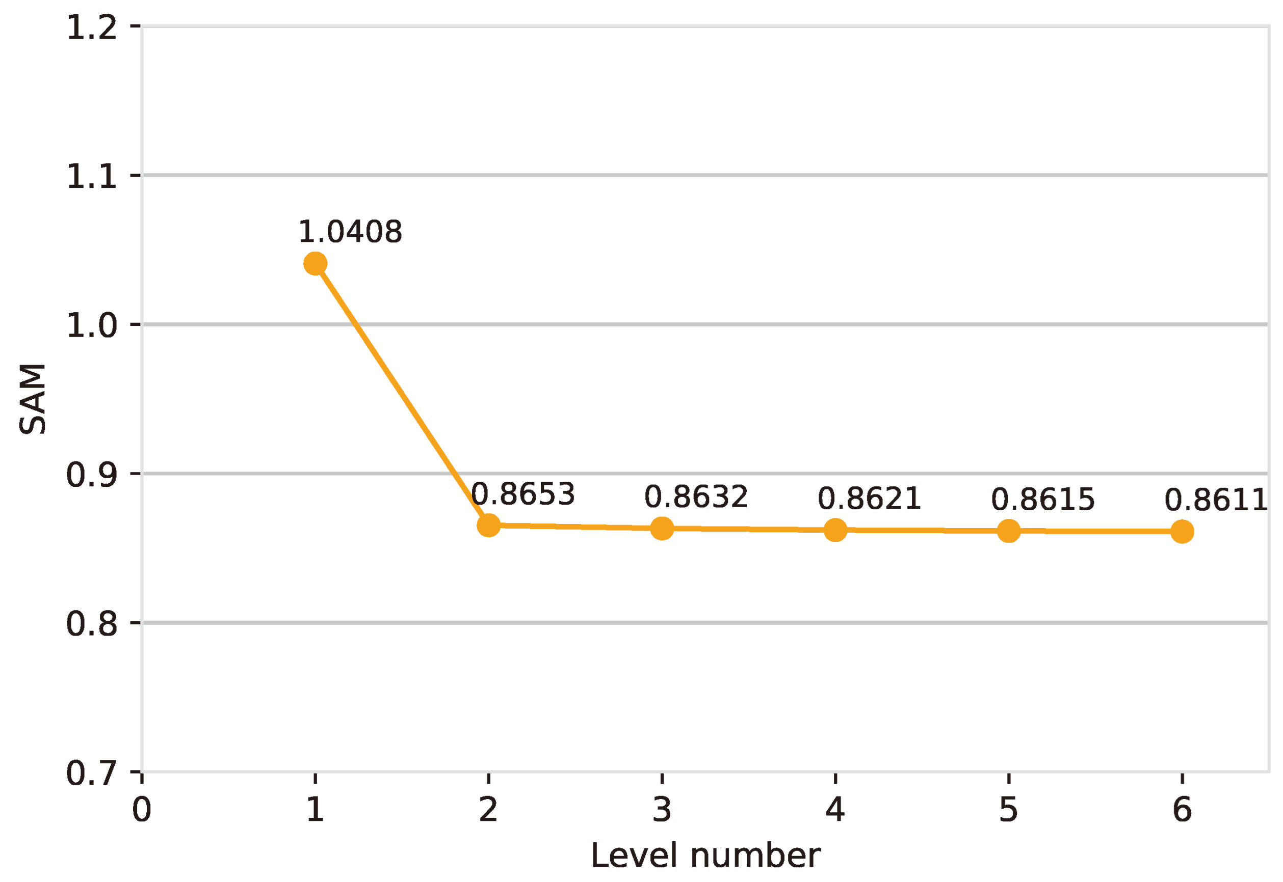
4.6. Ablation Experiments
5. Discussion
6. Conclusions
Author Contributions
Funding
Data Availability Statement
Acknowledgments
Conflicts of Interest
References
- Gilbertson, J.K.; Kemp, J.; Niekerk, A.V. Effect of pan-sharpening multi-temporal Landsat 8 imagery for crop type differentiation using different classification techniques. Comput. Electron. Agric. 2017, 134, 151–159. [Google Scholar] [CrossRef]
- Ye, Q.; Li, Z.; Fu, L.; Zhang, Z.; Yang, W. Nonpeaked Discriminant Analysis for Data Representation. IEEE Trans. Neural Netw. Learn. Syst. 2019, 30, 3818–3832. [Google Scholar] [CrossRef] [PubMed]
- Li, K.; Xie, W.; Du, Q.; Li, Y. DDLPS: Detail-Based Deep Laplacian Pansharpening for Hyperspectral Imagery. IEEE Trans. Geosci. Remote Sens. 2019, 57, 8011–8025. [Google Scholar] [CrossRef]
- Dadrass Javan, F.; Samadzadegan, F.; Mehravar, S.; Toosi, A.; Khatami, R.; Stein, A. A review of image fusion techniques for pan-sharpening of high-resolution satellite imagery. ISPRS J. Photogramm. Remote Sens. 2021, 171, 101–117. [Google Scholar] [CrossRef]
- Lu, H.; Yang, Y.; Huang, S.; Tu, W. An Efficient Pansharpening Approach Based on Texture Correction and Detail Refinement. IEEE Geosci. Remote Sens. Lett. 2022, 19, 1–5. [Google Scholar] [CrossRef]
- Zhou, X.; Liu, J.; Liu, S.; Cao, L.; Zhou, Q.; Huang, H. A GIHS-based spectral preservation fusion method for remote sensing images using edge restored spectral modulation. ISPRS J. Photogramm. Remote Sens. 2014, 88, 16–27. [Google Scholar] [CrossRef]
- Ghassemian, H. A review of remote sensing image fusion methods. Inf. Fusion 2016, 32, 75–89. [Google Scholar] [CrossRef]
- Choi, J.; Yu, K.; Kim, Y. A New Adaptive Component-Substitution-Based Satellite Image Fusion by Using Partial Replacement. IEEE Trans. Geosci. Remote Sens. 2011, 49, 295–309. [Google Scholar] [CrossRef]
- Chavez, P.S.; Kwarteng, A.Y. Extracting spectral contrast in landsat thematic mapper image data using selective principal component analysis. Photogramm. Eng. Remote Sens. 1989, 55, 339–348. [Google Scholar]
- Vivone, G.; Maranò, S.; Chanussot, J. Pansharpening: Context-Based Generalized Laplacian Pyramids by Robust Regression. IEEE Trans. Geosci. Remote Sens. 2020, 58, 6152–6167. [Google Scholar] [CrossRef]
- Zhou, J.T.; Civco, D.L.; Silander, J.A. A wavelet transform method to merge Landsat TM and SPOT panchromatic data. Int. J. Remote Sens. 1998, 19, 743–757. [Google Scholar] [CrossRef]
- Liu, J.; Basaeed, E. Smoothing Filter-based Intensity Modulation: A spectral preserve image fusion technique for improving spatial details. Int. J. Remote Sens. 2000, 21, 3461–3472. [Google Scholar] [CrossRef]
- Vivone, G.; Alparone, L.; Chanussot, J. A Critical Comparison Among Pansharpening Algorithms. IEEE Trans. Geosci. Remote Sens. 2015, 53, 2565–2586. [Google Scholar] [CrossRef]
- Cunha, A.L.; Zhou, J.; Do, M.N. The Nonsubsampled Contourlet Transform: Theory, Design, and Applications. IEEE Trans. Image Process. 2006, 15, 3089–3101. [Google Scholar] [CrossRef] [PubMed]
- Vivone, G.; Restaino, R.; Chanussot, J. Full Scale Regression-Based Injection Coefficients for Panchromatic Sharpening. IEEE Trans. Image Process. 2018, 27, 3418–3431. [Google Scholar] [CrossRef] [PubMed]
- Vivone, G.; Alparone, L.; Garzelli, A.; Lolli, S. Fast Reproducible Pansharpening Based on Instrument and Acquisition Modeling: AWLP Revisited. Remote Sens. 2019, 11, 2315. [Google Scholar] [CrossRef]
- Ballester, C.; Caselles, V.; Igual, L.; Verdera, J.; Rougé, B. A Variational Model for P+XS Image Fusion. Int. J. Comput. Vis. 2006, 69, 43–58. [Google Scholar] [CrossRef]
- Yang, Y.; Wu, L.; Huang, S.; Sun, J.; Wan, W.; Wu, J. Compensation Details-Based Injection Model for Remote Sensing Image Fusion. IEEE Geosci. Remote Sens. Lett. 2018, 15, 734–738. [Google Scholar] [CrossRef]
- Fang, F.; Li, F.; Shen, C.; Zhang, G. A Variational Approach for Pan-Sharpening. IEEE Trans. Image Process. 2013, 22, 2822–2834. [Google Scholar] [CrossRef] [PubMed]
- Liu, P.; Xiao, L.; Zhang, J.; Naz, B. Spatial-Hessian-Feature-Guided Variational Model for Pan-Sharpening. IEEE Trans. Geosci. Remote Sens. 2016, 54, 2235–2253. [Google Scholar] [CrossRef]
- Zhang, K.; Wang, M.; Yang, S.; Jiao, L. Convolution Structure Sparse Coding for Fusion of Panchromatic and Multispectral Images. IEEE Trans. Geosci. Remote Sens. 2019, 57, 1117–1130. [Google Scholar] [CrossRef]
- Huang, W.; Xiao, L.; Wei, Z.; Liu, H.; Tang, S. A New Pan-Sharpening Method With Deep Neural Networks. IEEE Geosci. Remote Sens. Lett. 2015, 12, 1037–1041. [Google Scholar] [CrossRef]
- Dong, C.; Loy, C.C.; He, K.; Tang, X. Image Super-Resolution Using Deep Convolutional Networks. IEEE Trans. Pattern Anal. Mach. Intell. 2014, 38, 295–307. [Google Scholar] [CrossRef] [PubMed]
- Masi, G.; Cozzolino, D.; Verdoliva, L. Pansharpening by Convolutional Neural Networks. Remote Sens. 2016, 8, 594. [Google Scholar] [CrossRef]
- Yang, J.; Fu, X.; Hu, Y.; Huang, Y.; Ding, X.; Paisley, J.W. PanNet: A Deep Network Architecture for Pan-Sharpening. In Proceedings of the IEEE International Conference on Computer Vision, Venice, Italy, 22–29 October 2017; pp. 1753–1761. [Google Scholar]
- Yuan, Q.; Wei, Y.; Meng, X.; Shen, H.; Zhang, L. A Multiscale and Multidepth Convolutional Neural Network for Remote Sensing Imagery Pan-Sharpening. IEEE J. Sel Top. Appl. Earth Observ. Remote Sens. 2017, 11, 978–989. [Google Scholar] [CrossRef]
- Deng, L.; Vivone, G.; Jin, C.; Chanussot, J. Detail Injection-Based Deep Convolutional Neural Networks for Pansharpening. IEEE Trans. Geosci. Remote Sens. 2021, 59, 6995–7010. [Google Scholar] [CrossRef]
- Zhang, T.; Deng, L.; Huang, T.; Chanussot, J.; Vivone, G. A Triple-Double Convolutional Neural Network for Panchromatic Sharpening. IEEE Trans. Neural Netw. Learn. Syst. 2021, 34, 9088–9101. [Google Scholar] [CrossRef] [PubMed]
- Tu, W.; Yang, Y.; Huang, S.; Wan, W.; Gan, L. MMDN: Multi-Scale and Multi-Distillation Dilated Network for Pansharpening. IEEE Trans. Geosci. Remote Sens. 2022, 60, 1–14. [Google Scholar] [CrossRef]
- Lei, D.; Huang, J.; Zhang, L.; Li, W. MHANet: A Multiscale Hierarchical Pansharpening Method With Adaptive Optimization. IEEE Trans. Geosci. Remote Sens. 2022, 60, 1–15. [Google Scholar] [CrossRef]
- Cheng, G.; Shao, Z.; Wang, J.; Huang, X.; Dang, C. Dual-Branch Multi-Level Feature Aggregation Network for Pansharpening. IEEE CAA J. Autom. Sinica. 2022, 9, 2023–2026. [Google Scholar] [CrossRef]
- Jian, L.; Wu, S.; Chen, L.; Vivone, G.; Rayhana, R.; Zhang, D. Multi-Scale and Multi-Stream Fusion Network for Pansharpening. Remote Sens. 2023, 15, 1666. [Google Scholar] [CrossRef]
- Lu, H.; Yang, Y.; Huang, S.; Chen, X. AWFLN: An Adaptive Weighted Feature Learning Network for Pansharpening. IEEE Trans. Geosci. Remote Sens. 2023, 61, 1–15. [Google Scholar] [CrossRef]
- Lu, H.; Guo, H.; Liu, R.; Xu, L.; Wan, W.; Tu, W.; Yang, Y. Cross-Scale Interaction With Spatial-Spectral Enhanced Window Attention for Pansharpening. IEEE J. Sel. Top. Appl. Earth Observ. Remote Sens. 2024, 17, 11521–11535. [Google Scholar] [CrossRef]
- Zhao, X.; Zhang, Y.; Guo, J.; Zhu, Y.; Zhou, G.; Zhang, W.; Wu, Y. Progressive Reconstruction Network With Adaptive Frequency Adjustment for Pansharpening. IEEE J. Sel Top. Appl. Earth Observ. Remote Sens. 2024, 17, 17382–17397. [Google Scholar] [CrossRef]
- Xiong, Z.; Liu, N.; Wang, N.; Sun, Z.; Li, W. Unsupervised Pansharpening Method Using Residual Network With Spatial Texture Attention. IEEE Trans. Geosci. Remote Sens. 2023, 61, 1–12. [Google Scholar] [CrossRef]
- Deng, L.; Vivone, G.; Paoletti, M.E.; Scarpa, G.; He, J.; Zhang, Y. Machine Learning in Pansharpening: A benchmark, from shallow to deep networks. IEEE Geosci. Remote Sens Mag. 2022, 10, 279–315. [Google Scholar] [CrossRef]
- Vivone, G.; Dalla Mura, M.; Garzelli, A.; Restaino, R. A New Benchmark Based on Recent Advances in Multispectral Pansharpening: Revisiting Pansharpening With Classical and Emerging Pansharpening Methods. IEEE Trans. Geosci. Remote Sens. Mag. 2021, 9, 53–81. [Google Scholar] [CrossRef]
- Alparone, L.; Wald, L.; Chanussot, J.; Thomas, C.; Gamba, P.; Bruce, L.M. Comparison of Pansharpening Algorithms: Outcome of the 2006 GRS-S Data-Fusion Contest. IEEE Trans. Geosci. Remote Sens. 2007, 45, 3012–3021. [Google Scholar] [CrossRef]
- Liu, X.; Wang, Y.; Liu, Q. Remote Sensing Image Fusion Based on Two-Stream Fusion Network. Conference on Multimedia Modeling. Inf. Fusion 2020, 55, 1–15. [Google Scholar] [CrossRef]
- Wang, Z.; Bovik, A.C. A universal image quality index. IEEE Signal Process. Lett. 2002, 9, 81–84. [Google Scholar] [CrossRef]
- Alparone, L.; Baronti, S.; Garzelli, A.; Nencini, F. A global quality measurement of pan-sharpened multispectral imagery. IEEE Geosci. Remote Sens. Lett. 2004, 1, 313–317. [Google Scholar] [CrossRef]
- Alparone, L.; Aiazzi, B.; Baronti, S.; Garzelli, A. Multispectral and panchromatic data fusion assessment without reference. Photogramm. Eng. Remote Sens. 2008, 74, 193–200. [Google Scholar] [CrossRef]


| Satellite | Band | Resolution (m) | Number of Training Images | Number of Validation Images |
|---|---|---|---|---|
| GaoFen-2 | LRMS | 4 | 19,809 | 2201 |
| PAN | 1 | |||
| QuickBird | LRMS | 2.44 | 17,139 | 1905 |
| PAN | 0.61 | |||
| WorldView-3 | LRMS | 1.2 | 9714 | 1080 |
| PAN | 0.3 |
| Method | SAM | ERGAS | CC | Q | Q2n |
|---|---|---|---|---|---|
| Reference | 0 | 0 | 1 | 1 | 1 |
| GS | 2.1482 | 2.4529 | 0.9693 | 0.9825 | 0.8469 |
| PRACS | 1.7781 | 1.7027 | 0.9859 | 0.9874 | 0.9236 |
| Wavelet | 1.9624 | 2.0984 | 0.9761 | 0.9796 | 0.8759 |
| HPF | 1.7716 | 1.7993 | 0.9843 | 0.9876 | 0.9135 |
| PNN | 1.1663 | 1.2583 | 0.9930 | 0.9941 | 0.9639 |
| MSDCNN | 1.0074 | 1.0629 | 0.9941 | 0.9955 | 0.9711 |
| FusionNet | 1.0439 | 1.1522 | 0.9933 | 0.9956 | 0.9658 |
| TDNet | 0.9170 | 0.8555 | 0.9964 | 0.9965 | 0.9790 |
| AWFLN | 0.8978 | 0.8191 | 0.9968 | 0.9966 | 0.9822 |
| SEWformer | 0.8775 | 0.8059 | 0.9966 | 0.9967 | 0.9823 |
| PRNet | 0.8881 | 0.8079 | 0.9969 | 0.9966 | 0.9824 |
| Proposed | 0.8653 | 0.7972 | 0.9969 | 0.9968 | 0.9823 |
| Method | SAM | ERGAS | CC | Q | Q2n |
|---|---|---|---|---|---|
| Reference | 0 | 0 | 1 | 1 | 1 |
| GS | 4.6296 | 7.0340 | 0.9393 | 0.9380 | 0.7617 |
| PRACS | 4.0177 | 6.5890 | 0.9456 | 0.9470 | 0.8194 |
| Wavelet | 4.8055 | 7.3663 | 0.9301 | 0.9294 | 0.7610 |
| HPF | 4.2084 | 6.6342 | 0.9454 | 0.9453 | 0.8074 |
| PNN | 3.9218 | 5.9846 | 0.9569 | 0.9569 | 0.8901 |
| MSDCNN | 3.7318 | 5.7833 | 0.9603 | 0.9601 | 0.8895 |
| FusionNet | 3.6742 | 5.7089 | 0.9585 | 0.9593 | 0.8864 |
| TD | 3.6608 | 5.7846 | 0.9569 | 0.9513 | 0.8501 |
| AWFLN | 3.6342 | 5.7399 | 0.9603 | 0.9601 | 0.8937 |
| SEWformer | 3.5948 | 5.5306 | 0.9619 | 0.9624 | 0.9005 |
| PRNet | 3.5750 | 5.7314 | 0.9621 | 0.9618 | 0.9011 |
| Proposed | 3.5110 | 5.3458 | 0.9626 | 0.9627 | 0.9012 |
| Method | SAM | ERGAS | CC | Q | Q2n |
|---|---|---|---|---|---|
| Reference | 0 | 0 | 1 | 1 | 1 |
| GS | 4.0384 | 3.8543 | 0.9553 | 0.9017 | 0.8584 |
| PRACS | 4.0031 | 3.4407 | 0.9579 | 0.9083 | 0.8812 |
| Wavelet | 5.281 | 4.4258 | 0.9321 | 0.8766 | 0.8361 |
| HPF | 3.9317 | 3.7153 | 0.9492 | 0.9111 | 0.8725 |
| PNN | 3.4077 | 3.7553 | 0.9427 | 0.9280 | 0.8881 |
| MSDCNN | 3.2809 | 3.8107 | 0.9430 | 0.9320 | 0.8858 |
| FusionNet | 3.2728 | 3.8245 | 0.9427 | 0.9321 | 0.8836 |
| TD | 3.3098 | 3.7089 | 0.9467 | 0.9337 | 0.8911 |
| AWFLN | 3.1754 | 3.3648 | 0.9572 | 0.9402 | 0.9111 |
| SEWformer | 3.2081 | 3.4954 | 0.9542 | 0.9370 | 0.9063 |
| PRNet | 3.2711 | 3.2866 | 0.9583 | 0.9385 | 0.9124 |
| Proposed | 3.1598 | 3.3370 | 0.9584 | 0.9408 | 0.9125 |
| GaoFen-2 | QuickBird | WorldView-3 | |||||||
|---|---|---|---|---|---|---|---|---|---|
| Method | QNR | QNR | QNR | ||||||
| Reference | 1 | 0 | 0 | 1 | 0 | 0 | 1 | 0 | 0 |
| GS | 0.8756 | 0.0683 | 0.0602 | 0.6439 | 0.0888 | 0.2934 | 0.8928 | 0.0159 | 0.0928 |
| PRACS | 0.8907 | 0.0355 | 0.0766 | 0.6837 | 0.0757 | 0.2603 | 0.8904 | 0.0259 | 0.0858 |
| Wavelet | 0.8699 | 0.0918 | 0.0422 | 0.6697 | 0.1491 | 0.2129 | 0.8586 | 0.0954 | 0.0509 |
| HPF | 0.9039 | 0.0468 | 0.0517 | 0.7424 | 0.0947 | 0.1799 | 0.9033 | 0.0303 | 0.0685 |
| PNN | 0.9825 | 0.0128 | 0.0048 | 0.8358 | 0.0508 | 0.1195 | 0.9436 | 0.0235 | 0.0337 |
| MSDCNN | 0.9814 | 0.0138 | 0.0049 | 0.8482 | 0.0703 | 0.0877 | 0.9545 | 0.0165 | 0.0295 |
| FusionNet | 0.9758 | 0.0159 | 0.0084 | 0.8818 | 0.0726 | 0.0492 | 0.9552 | 0.0114 | 0.0338 |
| TDNet | 0.9842 | 0.0102 | 0.0057 | 0.8877 | 0.0594 | 0.0562 | 0.9469 | 0.0232 | 0.0306 |
| AWFLN | 0.9823 | 0.0076 | 0.0102 | 0.8922 | 0.0578 | 0.0531 | 0.9559 | 0.0151 | 0.0295 |
| SEWformer | 0.9826 | 0.0126 | 0.0049 | 0.8967 | 0.0520 | 0.0541 | 0.9573 | 0.0119 | 0.0312 |
| PRNet | 0.9874 | 0.0074 | 0.0052 | 0.8983 | 0.0511 | 0.0533 | 0.9581 | 0.0131 | 0.0292 |
| Proposed | 0.9885 | 0.0071 | 0.0044 | 0.9070 | 0.0423 | 0.0529 | 0.9637 | 0.0087 | 0.0278 |
| Index | MSSCM | HFCEM | Double layer | SAM | ERGAS | CC | Q | Q2n |
|---|---|---|---|---|---|---|---|---|
| 1 | ✓ | ✓ | 1.2701 | 1.7005 | 0.9864 | 0.9935 | 0.9466 | |
| 2 | ✓ | ✓ | 0.9886 | 0.8942 | 0.9943 | 0.9957 | 0.9754 | |
| 3 | ✓ | ✓ | 1.0408 | 1.2261 | 0.9920 | 0.9946 | 0.9681 | |
| 4 | ✓ | ✓ | ✓ | 0.8653 | 0.7972 | 0.9969 | 0.9968 | 0.9823 |
Disclaimer/Publisher’s Note: The statements, opinions and data contained in all publications are solely those of the individual author(s) and contributor(s) and not of MDPI and/or the editor(s). MDPI and/or the editor(s) disclaim responsibility for any injury to people or property resulting from any ideas, methods, instructions or products referred to in the content. |
© 2025 by the authors. Licensee MDPI, Basel, Switzerland. This article is an open access article distributed under the terms and conditions of the Creative Commons Attribution (CC BY) license (https://creativecommons.org/licenses/by/4.0/).
Share and Cite
Huang, W.; Liu, Y.; Sun, L.; Chen, Q.; Gao, L. A Novel Dual-Branch Pansharpening Network with High-Frequency Component Enhancement and Multi-Scale Skip Connection. Remote Sens. 2025, 17, 776. https://doi.org/10.3390/rs17050776
Huang W, Liu Y, Sun L, Chen Q, Gao L. A Novel Dual-Branch Pansharpening Network with High-Frequency Component Enhancement and Multi-Scale Skip Connection. Remote Sensing. 2025; 17(5):776. https://doi.org/10.3390/rs17050776
Chicago/Turabian StyleHuang, Wei, Yanyan Liu, Le Sun, Qiqiang Chen, and Lu Gao. 2025. "A Novel Dual-Branch Pansharpening Network with High-Frequency Component Enhancement and Multi-Scale Skip Connection" Remote Sensing 17, no. 5: 776. https://doi.org/10.3390/rs17050776
APA StyleHuang, W., Liu, Y., Sun, L., Chen, Q., & Gao, L. (2025). A Novel Dual-Branch Pansharpening Network with High-Frequency Component Enhancement and Multi-Scale Skip Connection. Remote Sensing, 17(5), 776. https://doi.org/10.3390/rs17050776