Abstract
Sparse reconstruction-based imaging techniques can be utilized to solve forward-looking imaging problems with limited azimuth resolution. However, these methods perform well only under the traditional model for the platform with low speed, and the performance deteriorates for the maneuvering trajectory. In this paper, a structured Bayesian super-resolution forward-looking imaging algorithm for maneuvering platforms under an enhanced sparsity model is proposed. An enhanced sparsity model for maneuvering platforms is established to address the reconstruction problem, and a hierarchical Student-t (ST) prior is designed to model the distribution characteristics of the sparse imaging scene. To further leverage prior information about structural characteristics of the scatterings, coupled patterns among neighboring pixels are incorporated to construct a structured sparse prior. Finally, forward-looking imaging parameters are estimated using the expectation/maximization-based variational Bayesian inference. Numerical simulations validate the effectiveness of the proposed algorithm and the superiority over conventional methods based on pixel sparse assumptions in forward-looking scenes for maneuvering platforms.
1. Introduction
Forward-looking imaging radar (FIR) offers unique capabilities in both civil and military applications, operating effectively in all weather conditions, regardless of day or night. In traditional monostatic real aperture radar systems, wide bandwidth signals are transmitted to achieve range resolution, while the azimuth resolution is constrained by the physical aperture size. To overcome this limitation, synthetic aperture radar (SAR) employs a virtual aperture, which enhances the azimuth resolution [1,2]. However, the same Doppler history and small Doppler gradient make it challenging to accumulate the virtual aperture in FIR. Furthermore, the Doppler beam sharpening (DBS) method is not applicable in this case [3,4]. As a result, improving cross-range resolution becomes difficult when the scene is directly in front of the platform.
Notable research has been conducted on FIR. Monopulse forward-looking imaging based on angle measurement enables target angle estimation, which performs well for single-target scenarios [5,6]. However, this method cannot resolve multiple targets within the same beam. Bistatic SAR, with a specially separated configuration, increases additional Doppler information to overcome the FIR blind area and achieve high forward-looking resolution. Unfortunately, compared with monostatic SAR, bistatic SAR introduces greater system complexity, including challenges related to time, space, phase synchronization, and communication between the separated platforms [7,8,9,10,11].
To further enhance imaging performance, super-resolution imaging technology is employed to improve the azimuth resolution of FIR under platform constraints [12,13,14,15]. Considering the sparsity of certain typical radar scenes, sparse signal processing is utilized to achieve radar imaging. As is well known, radar echoes can be expressed as the convolution of the two-way antenna pattern and the scattering coefficients in the imaging scene [16]. By performing deconvolution, the scattering coefficients can be reconstructed. This can be formulated as a linear regression model , where the observed signal , the measurement matrix , and the sparse scatterings are incorporated, along with white noise [15,17,18,19,20]. As shown in Figure 1, sparse recovery is a classic method for linear regression, often referred to as - minimization. The black arrow denotes the explanation of the relevant vectors and the red arrow with the crosses indicates that sparse reconstruction is applicable to sparse scenarios rather than non-sparse ones.
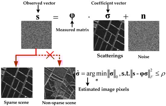
Figure 1.
Diagram of solutions to sparse recovery problem.
When the measurement matrix satisfies the restricted isometry property (RIP), the NP-hard -minimization problem can be simplified to -minimization, which can be solved using convex optimization algorithms. Typical convex optimization methods, such as basis pursuit (BP) [21] and the iterative soft thresholding algorithm (ISTA) [22], can address the deconvolution problem. However, the forward-looking imaging problem may not always satisfy the conditions for a convex function. Additionally, in imaging problems, these methods necessitate the selection and estimation of multiple hyperparameters, most of which rely on empirical values, thus posing challenges for their practical application. Recently, a spectrum estimation technique, known as the iterative adaptive approach (IAA), has been successfully applied to solve the optimization problem. Despite its success, IAA requires the computation of the covariance matrix inversion in each iteration. Moreover, some efficient IAA-based methods can reduce computational complexity, but this often comes at the cost of decreased reconstruction accuracy [16,23,24,25,26,27]. Greedy pursuit [28,29] is a widely accepted approach for sparse recovery due to its simple iterative structure. The sparse adaptive matching pursuit (SAMP) method is also frequently used to solve inverse problems, thanks to its adaptive sparsity parameters. However, these methods are prone to becoming stuck in local minima, which causes them to lose the global optimal solution, especially in complex forward-looking imaging scenarios [30].
In recent years, the Bayesian framework has been introduced to model the forward-looking sparse scene recovery problem. Compared with other sparse reconstruction methods, the Bayesian approach has the advantage of automatically learning model parameters, eliminating the need for manual adjustment based on different scenarios. The algorithm proposed in Reference [30], which relies on an atom matching process, is prone to falling into local extrema, reducing the algorithm’s robustness. In contrast, methods based on parameter estimation within the Bayesian framework are less likely to become caught in local optima, as they tend to seek a global optimal solution, thereby enhancing the stability of the reconstruction results. This highlights the fundamental differences in the concepts and structures between the two methods. Using an appropriate prior to model the scene can incorporate statistical information that enhances image quality. Sparse Bayesian learning (SBL), a classic Bayesian approach, models typical sparse signals with a Gaussian prior [31,32,33]. The maximum a posteriori (MAP) estimation, as a classic method for sparse signal recovery, avoids directly computing the analytical solution of the posterior for the variables. However, it faces the challenge of local minima and suffers from structural errors due to the neglect of posterior statistical information [34,35]. Additionally, existing Bayesian methods typically assume pixel sparsity for reconstruction, which overlooks the correlation between adjacent pixels. This omission of the image’s prior structural features leads to mismatch in complex forward-looking imaging scenarios.
Existing methods for achieving super-resolution imaging are not applicable to maneuvering trajectories, as the convolution model of the received echo only includes the antenna pattern and does not account for the Doppler phase. Reference [16] proposes a dictionary that incorporates Doppler information to accommodate the airplane platform, where both the Doppler phase and the antenna pattern are considered. The method can represent the geometry of moving platforms and improves the azimuth resolution of the image. However, it is not suitable for maneuvering platforms with curved trajectories. Due to the impact of three-dimensional (3D) acceleration introduced by the maneuverability of the platform, the over-complete dictionary matrix becomes inadequate for scene representation, leading to the failure of sparse reconstruction.
In this article, a super-resolution forward-looking imaging algorithm within the Bayesian framework, called the structured hierarchical Student-t (ST) prior with expectation/maximization (EM)-based variational Bayesian inference (SSTEM-VB) is proposed. This method utilizes an enhanced sparsity model for maneuvering platforms. First, the forward-looking imaging geometrical model and signal model for maneuvering platforms are derived. Based on these models, a virtual multi-domain phase compensation factor (MPCF) is introduced to compensate for 3D acceleration and range migration, thereby unifying and simplifying the high-order Doppler frequency. Next, the signal processing beam space is expanded to further enhance the sparsity of the signal. This leads to an optimized over-complete dictionary that matches the forward-looking imaging process with the enhanced sparsity model. Finally, a pattern-coupled hierarchical prior framework, which accounts for the dependencies between adjacent pixels and their corresponding coefficients, is designed to optimize the performance of forward-looking imaging.
The main superiority of the proposed algorithm can be summarized as follows:
- We establish an accurate mono-channel beam scanning geometry for FIR with maneuvering trajectories and form a high-dimensional beam space to enhance sparsity, thereby enabling Doppler deconvolution.
- We construct the MPCF to achieve error correction of joint envelope and phase introduced by the high-order motion of the maneuvering platform. Thus, an optimized convolution formulation with the accurate over-completed dictionary is derived.
- We propose a structured hierarchical framework, where the sparsity of each coefficient depends on its neighbors, to model the sparse signal. This prior helps avoid the “isolated coefficients” and encourages clustered features. An EM-based VB method is exploited to estimate the block sparse signal.
The remaining parts of this paper are organized as follows. The forward-looking geometrical model with maneuvering trajectory and signal processing model are established in Section 2. Section 3 describes the proposed SSTEM-VB algorithm with enhanced sparsity model in detail. In Section 4, the processing results of simulated experiments are designed to evaluate the proposed method. Finally, conclusions are drawn in Section 5.
2. Forward-Looking Imaging Convolution Model
2.1. Forward-Looking Imaging Geometric Model
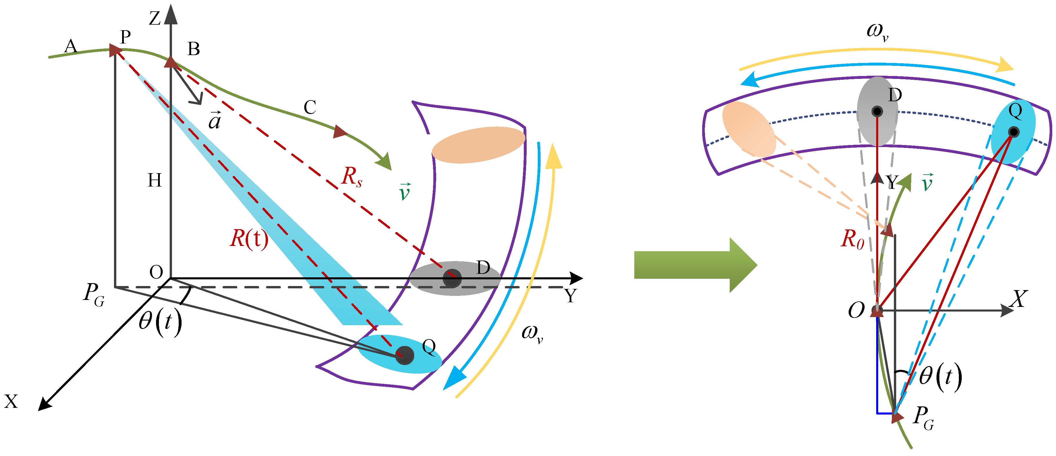
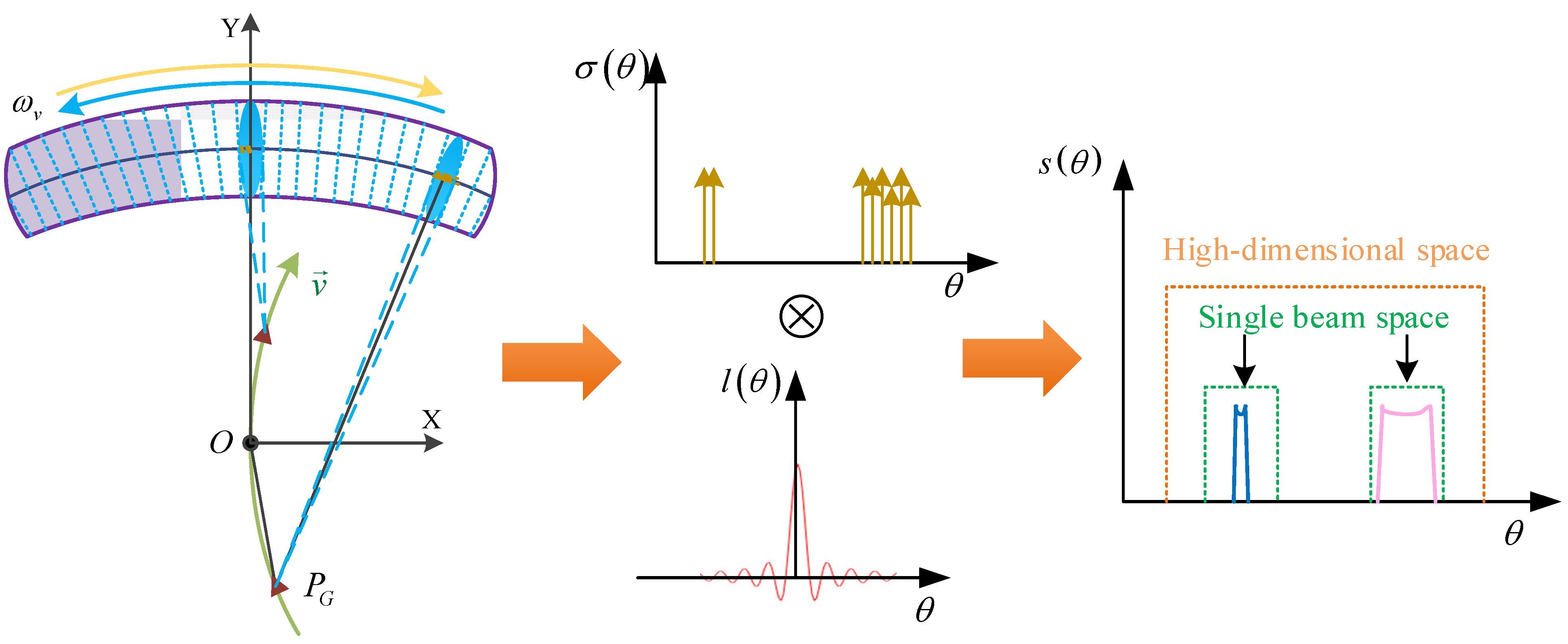
The forward-looking scanning structure with a maneuvering trajectory is constructed to illustrate the imaging geometric relationship, as shown in Figure 2. A Cartesian coordinate system Oxyz is defined, where point B represents the location of the platform at the midpoint of the acquisition period, and origin O is the projection of point B onto the ground. and are the altitude and slant range of point B. The maneuvering platform follows a curved trajectory with a 3D velocity and acceleration . The purple arc area in Figure 2 indicates the FIR scanning area, and the raw echo is obtained through steering operations with a scanning velocity . The y-axis represents the direction of horizontal velocity. The ellipsoidal regions in different colors represent the coverage area of the beam during the scanning. The yellow and blue arrows represent the direction of the beam scanning.
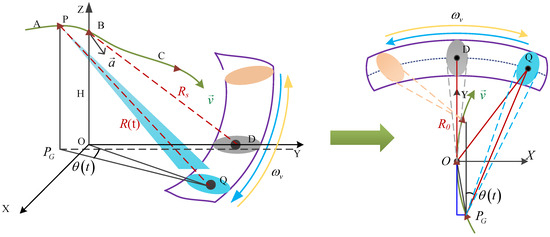
Figure 2.
Geometric model for maneuvering platform with curved trajectory.
Inspecting Figure 2, for any point P at an arbitrary location of the platform during its flight and any point Q in the forward-looking imaging area, the 3D coordinates of the vector in the imaging coordinate system can be represented as
where denotes the slow time, which describes the time variation between multiple transmitted pulses. and represent instantaneous azimuth angles. According to the sine theorem
where denotes the projection of point P on the ground, denotes the two-dimensional (2D) coordinates of point . The instantaneous slant range from the scattering coefficients in the target coordinate system to the maneuvering platform is then expressed as
where denotes the value of the vector, denotes the Maclaurin coefficients, which can be expressed as
where denotes the factorial operation of .
To express Maclaurin coefficients conveniently, three space angles are set up as
According to the space angles and Maclaurin expansion, the expression of can be then expressed as
2.2. Signal Model to Be Processed
Supposing the radar transmits linear frequency modulated (LFM) pulses, after demodulation, the baseband echo signal can be expressed as
where is the radar fast time, which refers to the sampling time within a single pulse when the radar receives echoes. and represent rectangular window function and antenna pattern, respectively. is speed of light, denotes the time delay, is the pulse width, denotes the carried frequency of radar, and is the LFM rate.
After pulse compression, the echo signal can be expressed as
where represents the transmitted bandwidth.
From (8), a convolution of the antenna pattern and scattering coefficients can be formed according to the echo in one range gate, which is expressed as
where denotes the convolution operator.
Considering the effect of noise , the echo in (8) can be rewritten as the matrix form
where represents the Hadamard product. denotes the received signal vector, M is the length of signal. denotes the unknown backscattering coefficients vector to be reconstructed. is the length of the target vector. denotes the pulse repetition frequency (PRF) and is the scanning extent. denotes the Doppler phase in (8). The discrete antenna pattern matrix is designed based on the radar beam steering, as shown below
where denotes the sampling value of the antenna pattern vector, and represents the effective sampling length of the antenna pattern vector.
The conventional Doppler phase matrix is based on the assumption that the range cell migration is much less than the center slant range, which can be expressed as
where is the instantaneous Doppler centroid, and denotes the pitch angle.
From (10), it is noted that the conventional Doppler convolution model takes both the antenna pattern and the Doppler information into consideration, which contributes to the reconstruction and results with better performance than the traditional convolution model that neglects the Doppler phase. However, this model does not account for the high maneuverability of the platform, which leads to a mismatch between the over-complete dictionary and the sparse reconstruction operator in forward-looking scenes. Therefore, to achieve precise reconstruction of forward-looking scenes, a structured Bayesian super-resolution forward-looking imaging algorithm under the modified Doppler model with enhanced sparsity will be discussed in the next section.
3. Bayesian Forward-Looking Super-Resolution Imaging with Enhanced Sparsity
In this section, we first design the MPCF to perform the pre-processing operation. Then, an optimized Doppler convolution model with enhanced sparsity is constructed. Finally, a Bayesian forward-looking imaging algorithm, incorporating a structured hierarchical ST distribution prior, is described in detail.
3.1. Optimization of Doppler Convolution Model with Enhanced Sparsity
The range walk and the higher-order phase brought by the high-order motion in the maneuvering trajectory make sparse recovery of forward-looking area inefficient. Observing the expansion in (6), the relative term for 3D acceleration appears in the high-order phase. Additionally, elements of over-complete dictionary matrix are zero in every column where the beam is not illuminated, as indicated by the model (10). To decouple the range and azimuth and compensate precise high-degree maneuverability, a virtual MPCF is designed in different domains, which can achieve satisfactory forward-looking imaging performance.
We can separate the Maclaurin expansion from (6) that contains the 3D acceleration, and it can be represented as
Considering the particularity of the measurement matrix, a compensation factor is constructed to eliminate 3D acceleration components, which is expressed as
After compensating for the high-order phase introduced by 3D acceleration, the remaining phase in range frequency and slow time domain is expressed as
where , , and denote the high-order expansions in (6) that do not contain 3D acceleration terms.
Subsequently, a range migration correction factor is designed to achieve the compensation, which is expressed as:
After compensation with the MPCF in different domains, the pre-processed signal in 2D time domain is expressed as
where the compensated slant range in the envelope and phase can be formulated as
Noting that the first-order term, which is compensated in the envelope, is retained in the phase. Since the Doppler frequency on the left and right sides is symmetrical, and the influence of maneuverability is reflected in both envelope and phase, the compensation for Doppler, i.e., the first-order term, occurs only in the envelope. On the other hand, compensation for the high-dimensional motion of the maneuvering platform needs to be reflected in both the envelope and the phase. The difference between them is evident in their respective slant range. Moreover, the compensation for the 3D acceleration reflected in the high-order phase is achieved in the 2D time domain and range walk correction is accomplished in the range frequency and slow time domain. The MPCF thus virtually exists across different domains, enabling the joint compensation of both envelope and phase.
As we know, optimizing the over-complete dictionary matrix is essential for describing accurately forward-looking imaging. After compensating with the MPCF, the variation, containing both spatial beam scanning and phase correction, should be reflected in the measurement matrix, and it can be modified as
where represents the extension of to all azimuth angles . And denotes the change of the slow time.
Sparse imaging can be utilized to boost the performance of forward-looking imaging. However, in complex forward-looking scenarios, the scatter distribution may not adhere to the sparsity assumption, especially when scatters are concentrated within one beam space, the super-resolution performance is seriously reduced. Therefore, applying directly the sparse imaging to the forward-looking scenes presents some obstacles and limitations.
The forward-looking scene can be divided into multiple beam spaces, as the maneuvering platform scans the forward region, as shown in Figure 3. The blue ellipsoidal regions represents the coverage area of the beam during the scanning. The number of beam spaces is equivalent to the number of wave digits. Therefore, the targets in the scene can be viewed as the spatial samples captured by the FIR in the beam space during the beam steering process.
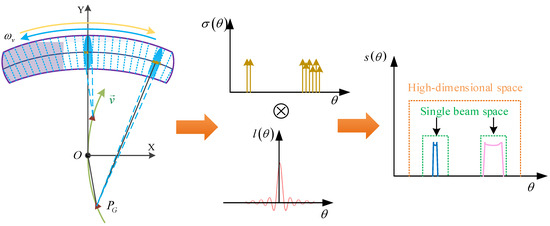
Figure 3.
Forward-looking imaging model with enhanced sparsity.
If the scattered points only occupy a portion of the space within a single beam, it can be considered that the local scene is sparse in that space. However, as shown by the pink curve in the green space of Figure 3, in most cases, multiple scatters in the scene occupy the majority of the green rectangular space. To enhance sparsity, a higher-dimensional space is formed by expanding the single beam space. This merging operation reduces the relative number of spatial scatters within the single beam, thereby achieving enhanced sparsity in forward-looking scenarios. Assuming that the scatters taking up most of the original low-dimensional space are limited and only occupy a small portion of the expanded space, as shown by the orange rectangle in Figure 3, we can consider the scattering points to be recovered in the fused beam space as sparse. The enhanced sparsity ultimately leads to better reconstruction results.
Based on the merging and expansion of the beams, the expanded single beam space becomes equivalent to the original multi-beam space, broadening the new single beam space. The high-dimensional beam space is obtained to enhance sparsity of the forward-looking scene. Subsequently, the linear regression model for one range gate under the enhanced sparsity model can be expressed as
Then, the azimuth signal in the modified model with enhanced sparsity, referred to as the enhanced sparsity model, for one range gate can be expressed as
where denotes the number of beams after the expansion operation, and represent the expanded echoes and scattering points in the high-dimensional space, respectively. denotes the expand measurement dictionary matrix, which is given as
3.2. Hierarchical Prior Model for Forward-Looking Imaging
For the forward-looking imaging method presented in this paper, azimuth super-resolution depends on sparse reconstruction operators. Sparse recovery theory is employed to solve the ill-conditioned linear inverse problem. It is effective to mine the prior information for enhancing the forward-looking imaging performance.
In this subsection, a sparse prior, serving as additional information, of the forward-looking scene is generally utilized to achieve the desired super-resolution image. From a Bayesian perspective, the sparse reconstruction problem can be solved through prior modeling and estimation of the relevant parameters. As we know, the hierarchical prior is better suited for complex forward-looking scenes; the hierarchical ST prior is thus designed to model the scene.
To conveniently facilitate the derivation of the formula, real numbers are selected, which does not affect the overall algorithm framework or conclusions, as performed by other research teams [36]. According to the Bayesian criterion, the sparse characteristic of the scanning scene can be accurately modeled by using different sparse priors for both the observations and scenes. The prominent scatters tend to distribute sparsely across the entire scene. Accurate probabilistic modeling of the backscattering coefficients in reconstructed scenes can enhance the imaging performance within the sparse Bayesian framework.
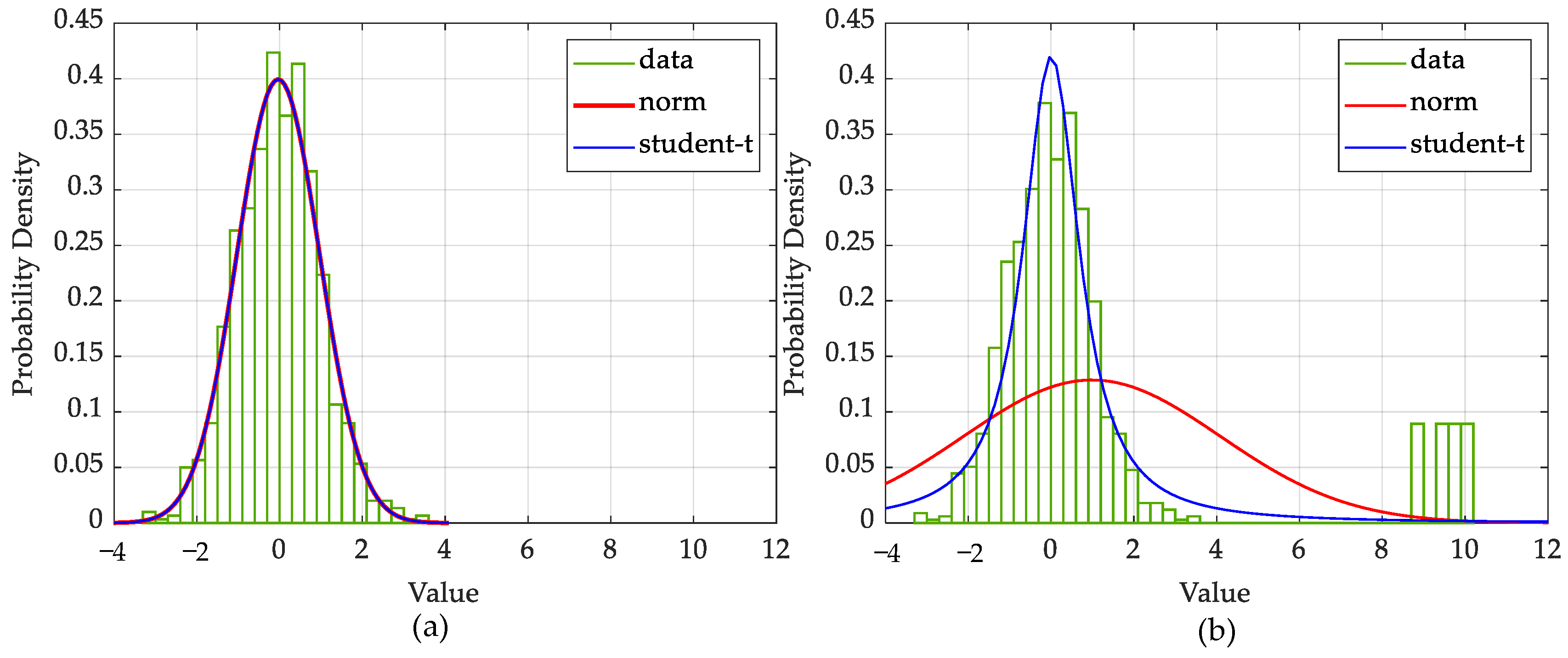
In the preliminary cognition, Gaussian distribution is generally exploited to model the image. However, in typical forward-looking scenes, targets of interest exhibit high pixel values, while a large number of scatters are represented as background noise with low pixel values. In this case, the Gaussian distribution is not well suited to fit these outliers, which will seriously degrade imaging performance. To address this problem, the ST distribution, which is more robust to outliers, is introduced to model the forward-looking scene [37]. The probability density function (PDF) of the ST distribution has higher tails and a narrower peak compared with the Gaussian distribution.
To verify the feasibility of using the ST distribution as a sparse prior, Figure 4 compares the fitting solutions for the Gaussian and ST distributions. In Figure 4a, the fitting solutions for data without outliers using both distributions are equally satisfactory. From Figure 4b, however, we see that the ST distribution is more adaptable to the outliers than the Gaussian, which is significantly disturbed by outliers, leading to a less accurate fitting solution. The ST prior can be thus expected to offer better performance in sparse representation and regression than the Gaussian.
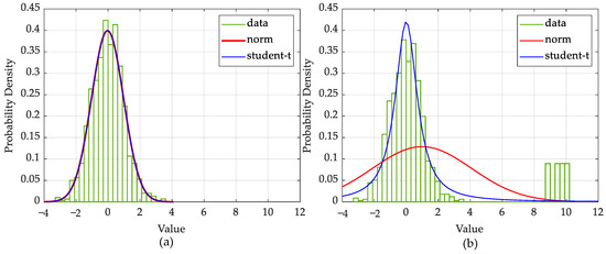
Figure 4.
Illustration of the robustness of ST distribution compared with Gaussian. (a) Histogram distribution of some data points drawn from a Gaussian distribution, together with the fit obtained from a Gaussian (red curve) and an ST distribution (blue curve). (b) Some data points drawn from a Gaussian distribution with some outliers, together with the two fit curves.
Therefore, the ST prior is exploited to model the signal, and the precision parameter is carefully designed to follow the Gamma distribution. The precision parameter represents the inversion of the covariance matrix in a multidimensional Gaussian PDF and is more convenient than the variance variable. Moreover, a hierarchical prior with two layers may perform better than using the ST distribution alone.
The noise is generally supposed to be ST distribution, which is modeled as:
where is the noise precision, the scaling parameters are generally set to be small to make the prior of non-informative, and is the degree of freedom. Then, let the Gamma density be denoted by , defined as , is the Gamma function, denotes the Gaussian distribution.
Combining the regression model with the excitation noise distribution, the likelihood of the observed signal can be expressed as
At this point, this distribution can be rewritten as
where , represents latent variables that modify the precision for each observation and is the diagonal matrix whose elements are defined by the vector. Then, the precision is commonly assumed to be a Gamma distribution
Finally, the model is completed by assigning a Gamma prior with distinctive scaling parameters to the degrees of freedom :
Based on the assumption of the sparse forward-looking scene, the target scattering coefficient, assumed to follow an ST distribution, is modeled as
Noting that, the latent variable can be modeled as Gamma distribution
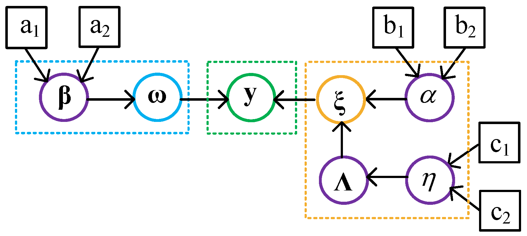
Similarly, as with setting the parameters , the scaling parameters are generally initialized to the small value for the non-informative prior. It is worth nothing that the real forward-looking scene can be regarded as being composed of numerous targets. The graphical model and the interdependency between the model parameters are shown in Figure 5.

Figure 5.
Graphical model.
In this graphical model, the squared black nodes correspond to hyperparameters, the green-circled node represents the observed random variable, the nodes with purple circles denote the latent random variables, and the blue-circled and orange-circled nodes represent the scattering and noise random variables, respectively, and the black arrows denote the relationship of representation between variables and parameters.
3.3. Variational Bayesian Inference for Estimatin Variables
After prior probability modeling, some techniques are utilized to estimate the posterior distribution of the forward-looking imaging parameters, including the scattering coefficients and other Bayesian modeling variables . In this subsection, the VB inference is applied to the observations, backscattering coefficients, and other latent variables to derive sparse signal recovery under the hierarchical ST framework. Unlike MAP estimation, this technique analytically calculates the posterior of all variables. It searches for the minimum Kullback–Leibler (KL) divergence between the real posterior distributions and the approximated one to estimate the parameters .
The VB interference approximates the posterior by factorizing over groups of parameters , which are assumed to be independent of each other. Since KL divergence is non-negative and can only be zero if equals , the approximated posterior can be calculated as
The solution to the approximate posterior using VB inference is given by
where denotes the expectation of the function with respect to the approximate posteriors of all random variables in except . is one of the elements in parameter , is a constant independent of .
Let
where denotes the expectation . It can be observed that the derived posterior follows a new Gamma distribution
where
Let
It is not analytically tractable to determine a joint distribution for , so is applied to the same procedure individually to obtain the posterior
where
Let
It can be seen that the posterior does not correspond to any standard distribution because of . Therefore, we bring up Stirling’s approximation to approximate the inference as
which can also be recognized as a Gamma distribution
where
Let
The above posterior is quadratic to , so it can be regarded as a Gaussian
where
Finally, let , applying the procedure for , it can be obtained as
The posterior of precision follows a Gamma distribution
where
Obviously, the closed-form algebraic solutions for these coefficients cannot be derived, as each approximation of the posterior above depends on the expectations of the others. However, solutions can be obtained by initializing the expectations or the priors, and then updating iteratively the estimation of hyperparameters, until convergence. The expectations related to are given as
respectively, where is the digamma function, denotes the trace operator, together with the expansion
3.4. Statistical Structured Sparsity Hierarchical Model
In the previous subsection, the hierarchical model was constructed to represent the forward-looking imaging scene, assuming the image to be pixel sparse. However, motivated by the observation that areas with nonzero pixels are usually contiguous, it is noted that a pixel with zero value is typically surrounded by other zero-valued pixels. This suggests that the prior scenarios should be modeled as structured sparsity. In this case, the precision of each pixel in the scene depends not only on its own hyperparameter, but on those pixels around it. The sparsity patterns of the coefficients in the neighboring region are statistically dependent.
Therefore, a structured Bayesian model is proposed to represent precisely sparse signals, making it more adaptable to forward-looking scene targets with block structures. Subsequently, an EM-based VB method is introduced to achieve the estimation of the scattering coefficients.
To represent the degree of dependence and pattern relevance between adjacent pixels, a structural coefficient is defined. It is apparent that the pattern-coupled prior reduces to the pixel sparse one (30) as . In this case, based on the structured hierarchical model, a prior over is expressed precisely as
In this time, the sparse patterns of adjacent coefficients are coupled through their shared structural coefficient. Meanwhile, the hyperparameters, during the iteration process, are dependent on each other through their commonly connected coefficients. Such a pattern-coupled hierarchical model has the potential to yield structured sparse solutions for forward-looking scenes, without imposing any pre-defined structures on the recovered scenarios. It allows the model to automatically adapt to the block sparse structure.
Under the assumption of joint sparsity, the mean and covariance of the posterior are updated as
Regretfully, the modified priors placed over make it challenging to derive a full VB inference. Therefore, the EM algorithm is utilized to estimate the set of hyperparameters , employing two iterative steps: the E-step and the M-step.
E-step: It requires computing the expectation of the complete posterior with respect to the hidden variable . And the Q function in this step is given as
Ignoring the term that is independent to , the function in (60) can be re-expressed as
M-step: The new estimate of is updated by maximizing the Q function achieved in the E-step,
A conventional strategy for maximizing the Q function is to optimize the parameters independently. In this case, however, the hyperparameters in the Q function are entangled due to the term . As a result, it is challenging to analytically obtain the optimization. An analytical sub-optional solution can be computed using Gradient descent methods in virtue of specific techniques.
The first derivative of with respect to is obtained as
To overcome the coupling problem and search for a suboptimal solution to this optimization, a commonly used technique is to assume that the same precision is modeled for the adjacent pixels . This hypothesis has been widely applied to sparse reconstruction within the Bayesian framework. For surface targets with block sparsity, the correlation between scatters in the neighborhood can be represented by adjacent pixels sharing the same precision [38]. Based on this assumption, the gradient can be simplified as
Forcing the derivatives (64) to zero, the suboptimal solution for is updated as
It is noted that the negative feedback mechanism, where large coefficients tend to suppress the value of , keeps decreasing most of the zero entries in until they become negligible. As a result, only a few prominent entries survive to explain the sparse scene. This process eventually leads to a structured sparse solution through iterations. Algorithm 1 summarizes the detailed flow of the procedure.
| Algorithm 1: SSTEM-VB |
| Input: the observation , dictionary matrix Output: sparse approximation of the target signal |
| Initialization: the targets’ scattering coefficient , ; During the iteration Repeat , , using (59); Update , using (65); , using (55), (56); Update , using (52); Update , using (51); until halting criterion true return |
Assume that the echo matrix has a dimension of (azimuth × range) and the over-completed dictionary matrix has a dimension of , with the algorithm iterating times. The computational complexity of operations such as element-wise updates of , independent matrix conjugate transposition, and other parameter updates do not involve cubic complexity. Therefore, these low-complexity operations are negligible. The primary computational complexity of the algorithm lies in the solution of the scattering coefficient variable , which costs . Based on this analysis, it is evident that the proposed method improves sparse reconstruction performance but comes at the cost of increased computational complexity.
4. Simulation Results and Discussion
In this section, several experimental simulations are conducted to verify the efficiency of the proposed SSTEM-VB method with the enhanced sparsity model. Performance comparisons between ISTA, SAMP, SBL, and the proposed SSTEM-VB methods are designed based on experimental simulations under different signal-to-noise ratio (SNR) conditions and processing models. Moreover, the scanning grid is uniform in azimuth for all approaches considered in the target simulations.
SNR is defined as follows
where and denote the mean power of the noise and the signal, respectively.
4.1. Point Target Simulation
In this subsection, we design the simulations with point-scattering targets to evaluate the superiority of the proposed method in this paper.
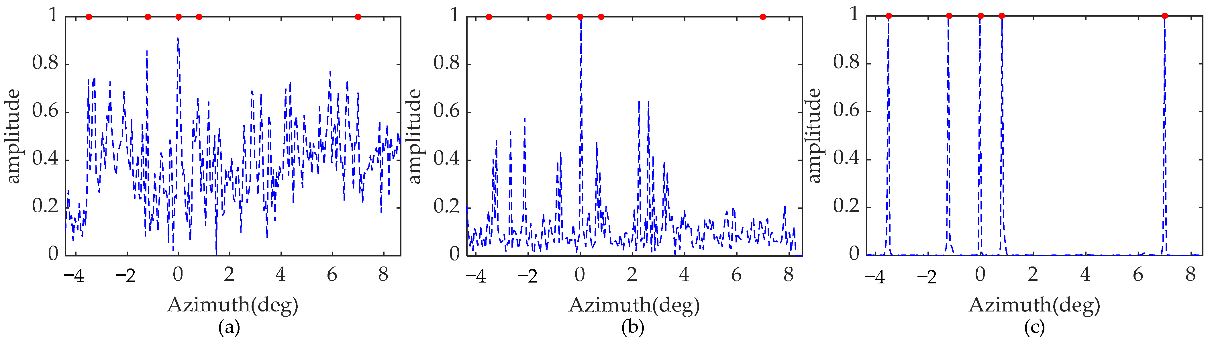
Five point targets with the same normalized amplitude, located at −3.5°, −1.2°, 0°, 0.8°, and 7°, are considered in this simulation. It is designed to verify the necessity of the constructed MPCF. White Gaussian noise with an SNR of 20 dB is added to the signal. The red circles represent the initial normalized amplitude and the blue dotted lines show the recovery results. Furthermore, the simulated results are based on 15 Monte Carlo trials.
As shown in Figure 6, the red dots denote the true location and amplitude of the point targets. In Figure 6a, point targets cannot be recovered due to the mismatch in the dictionary caused by the high-order maneuverability of the platform, which disrupts the sparse recovery. Inspecting Figure 6b, few scattering points can be reconstructed, and the false targets appear. It is evident that conventional Doppler phase compensation fails to produce a satisfactory forward-looking image. In contrast, using the proposed whole pre-processing operation, the five targets are well focused with accurate locations and amplitudes, as shown in Figure 6c. Moreover, the sidelobes of the reconstructed points decay rapidly. This simulation demonstrates that the constructed MCPF achieves accurate phase correction, and with the pre-processing operation, the high azimuth resolution can be increased by the proposed algorithm for maneuvering platforms.

Figure 6.
Reconstruction results with proposed method with different processes. (a) without compensation. (b) with conventional Doppler phase compensation. (c) with the whole process.
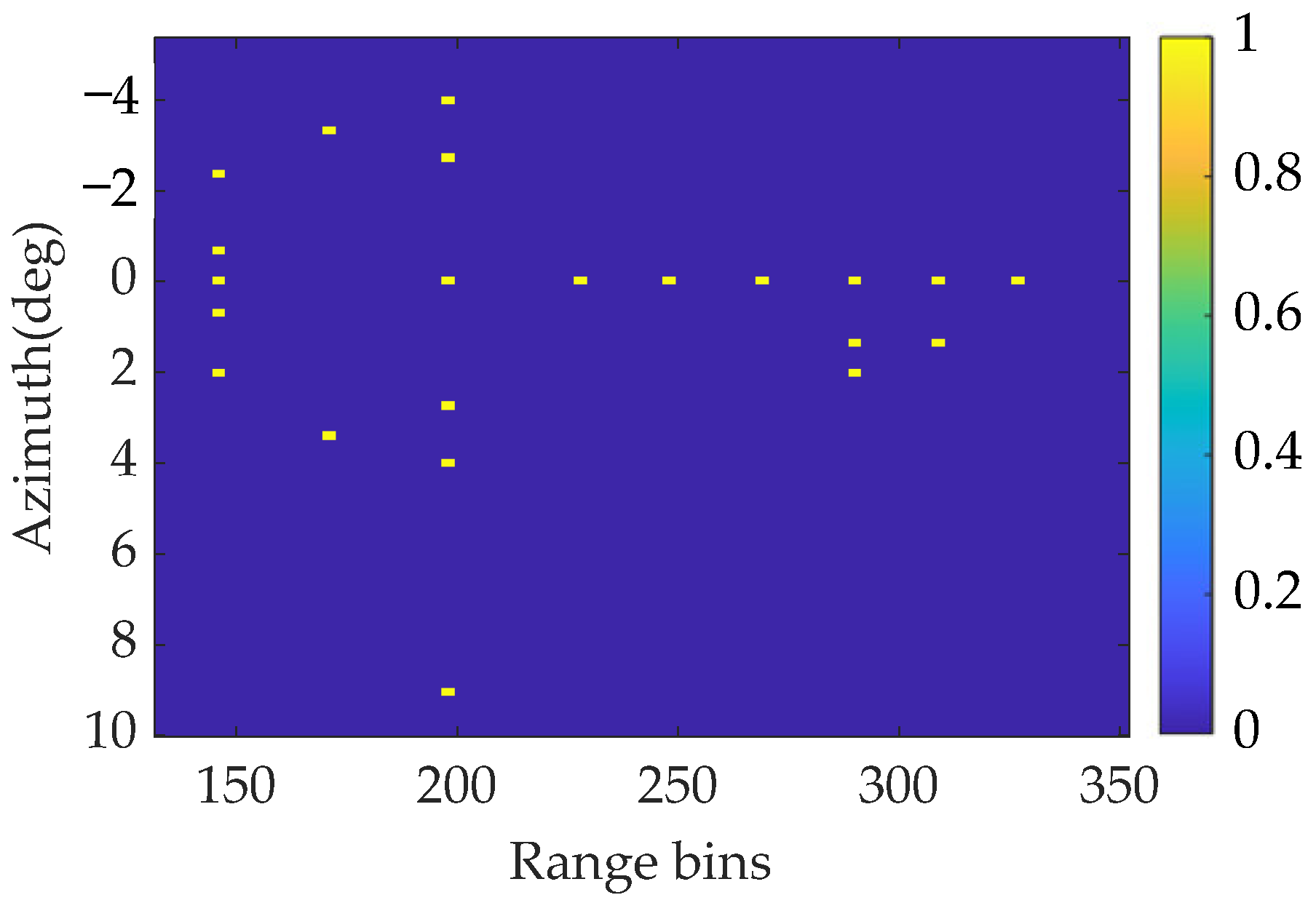
Then, a simulated scene consisting of some independent point targets with normalization amplitude is considered. The original scene is shown in Figure 7. To verify the super-resolution effect of the proposed method, the minimum angular interval between two points is set to 1.3°, which is smaller than the beamwidth. In addition, the signal contains white Gaussian noise with an SNR of 18 dB. Performed simulation parameters for the point targets are shown in Table 1.
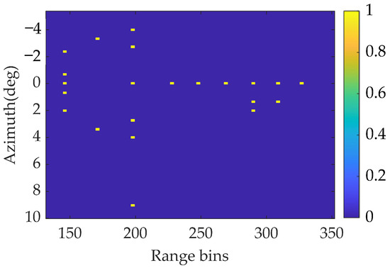
Figure 7.
Actual forward-looking image in point target simulation.

Table 1.
Simulation parameters of point targets.
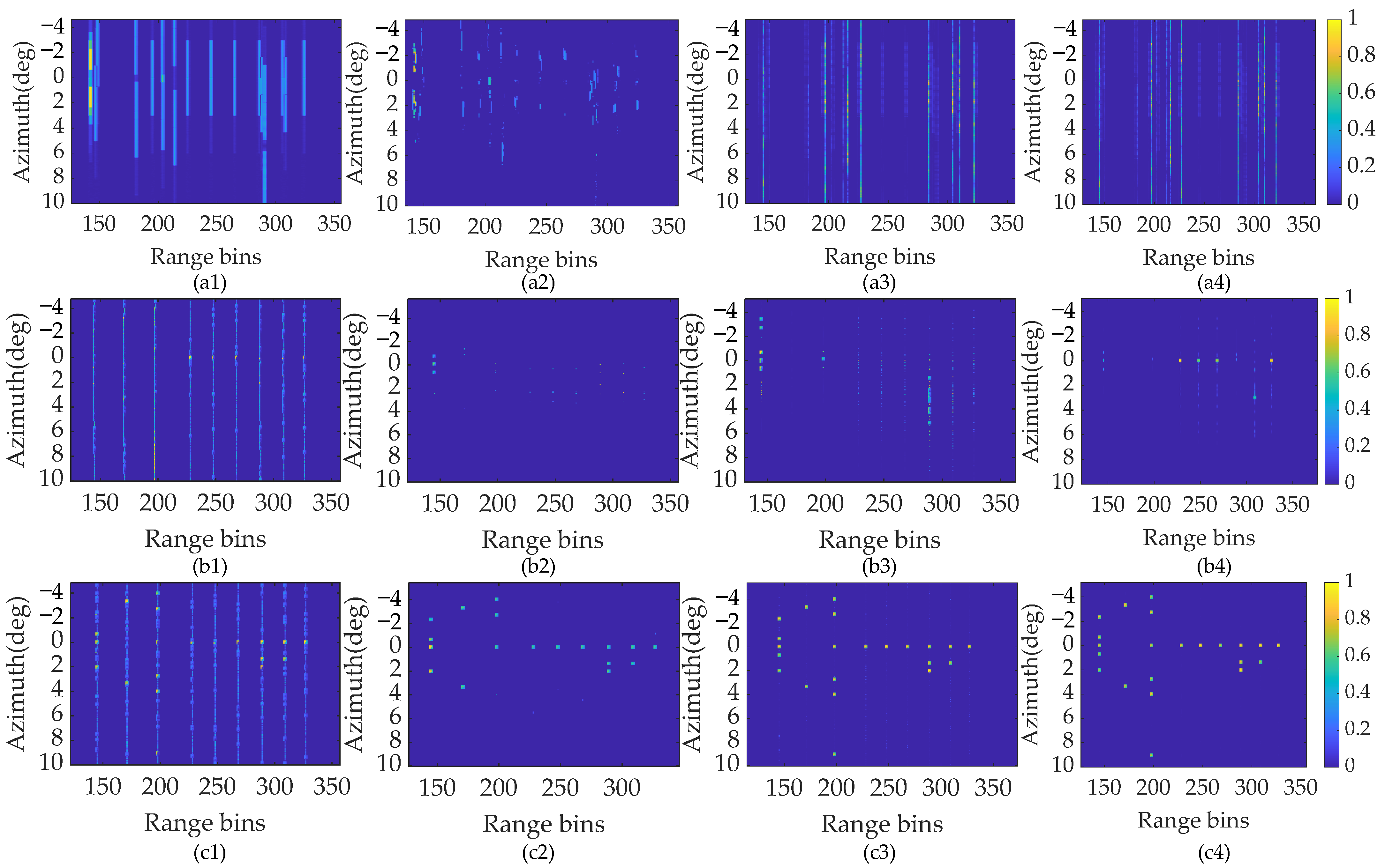
The super-resolution results using different alternative reconstruction methods, including the ISTA, SAMP, SBL, and the proposed SSTEM-VB methods using three processing models are shown in Figure 8.
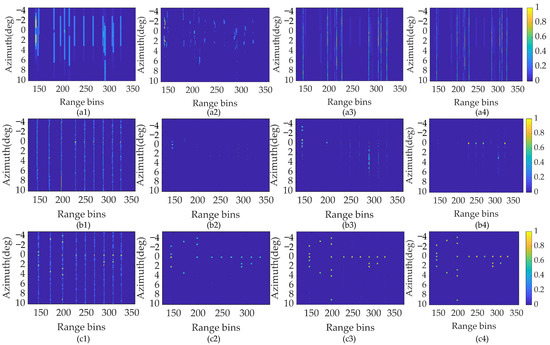
Figure 8.
Point target super-resolution results. (a1) ISTA method. (a2) SAMP method. (a3) SBL method. (a4) SSTEM-VB method with traditional model. (b1) ISTA method. (b2) SAMP method. (b3) SBL method. (b4) SSTEM-VB method with conventional Doppler model. (c1) ISTA method. (c2) SAMP method. (c3) SBL method. (c4) SSTEM-VB method with proposed enhanced sparsity model.
Inspecting Figure 8(a1–a4), under the traditional convolution model, the point targets cannot be recovered with the proposed method or the other three comparison methods. It highlights that the Doppler information brought by the relative motion is indispensable for the maneuvering platform. Figure 8(b1–b4) show the reconstruction results of the compared methods using the conventional Doppler convolution model. Under this model, the regression performance of the above four methods is improved, but still remains unsatisfactory. The comparison images of these methods with the enhanced sparsity model are shown in Figure 8(c1–c4). Apparently, the reconstruction of these methods has been enhanced for all methods. In the result recovered by the ISTA method, some targets can be distinguished, but severe blurring and false targets appear. The imaging performance is increased by the SAMP method, but it also leads to a loss in the amplitude of targets, and, in certain cases, the targets themselves are lost due to the dilemma of local minima. The SBL method can recover all targets other than the two closed targets, but it introduces several transverse ripples and sidelobes. On the contrary, the proposed SSTEM-VB method reconstructs all targets accurately with satisfactory amplitudes and few transverse ripples. These results show that the proposed method based on the enhanced sparsity model can handle complex forward-looking imaging problems.
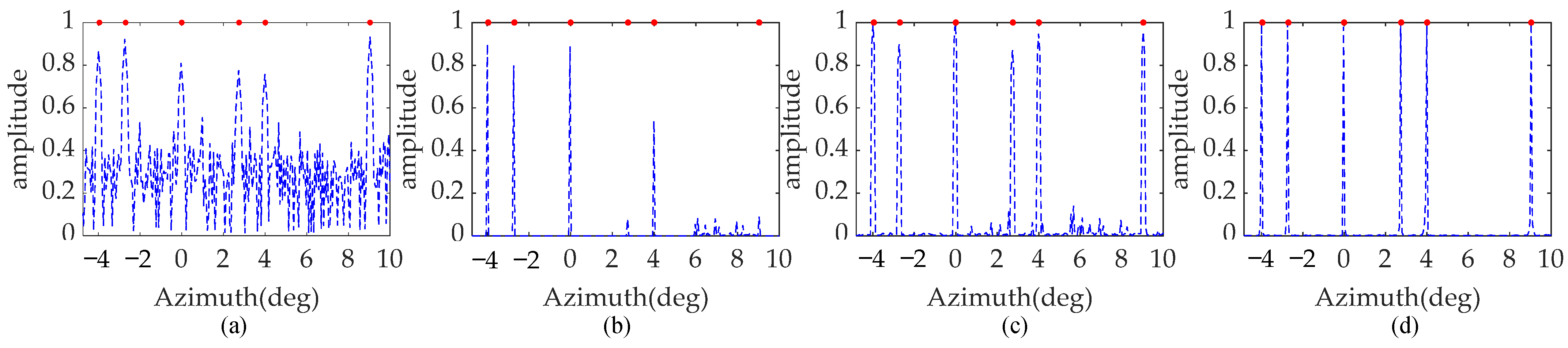
To compare clearly the reconstructed performance of the above methods with the enhanced sparsity model in detail, the profiles in the same range unit 198 from all four methods are shown in Figure 9. From Figure 9a, the ISTA profile shows coarse performance, as it fails to completely distinguish the point targets due to severe transverse ripples and sidelobes. In Figure 9b, the SAMP profile achieves better performance, but it still suffers from some false targets and missing targets. Almost all targets can be recovered in the SBL profile, as shown in Figure 9c. Regretfully, the amplitude of some targets is deficient, and several sidelobes are not satisfactory. In contrast, inspecting Figure 9d, SSTEM-VB can accurately reconstruct adjacent or edge point targets. It is apparent that the SSTEM-VB method outperforms the ISTA, SAMP, and SBL methods in forward-looking imaging.
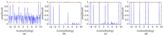
Figure 9.
Point scattering target profiles at range unit 198. Result processed by (a) ISTA method, (b) SAMP method, (c) SBL method, (d) proposed SSTEM-VB method.
To further quantitatively analyze the superiority of the proposed SSTEM-VB method compared with the other three methods, two important indexes, mean square error (MSE) [35] and image entropy, are introduced to quantify the imaging performance. MSE is defined as follows:
where and denote the reconstructed image and the real image, is the total number of Monte Carlo trials. In the simulations, the value of is 200.
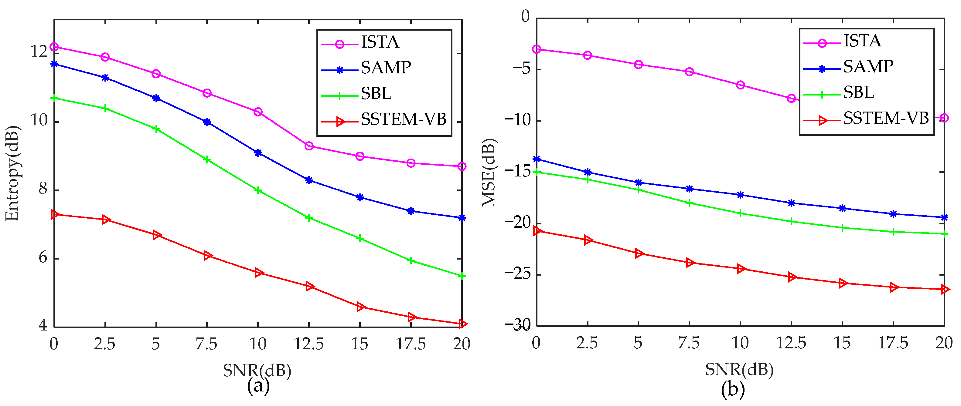
It is wise to calculate only the MSE and image entropy for the four algorithms with the enhanced sparsity model, given the coarse and blurred imaging performance under the traditional convolution model and conventional Doppler convolution model, which use unsuitable Doppler information. Figure 10 shows the MSE and image entropy curves under different SNRs for the various methods.
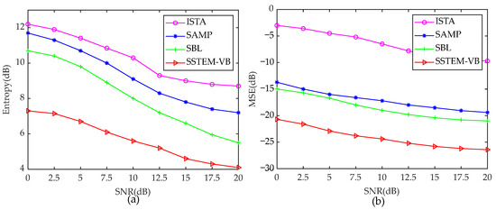
Figure 10.
Entropy and MSE curves under different SNRs based on different methods. (a) Entropy curves. (b) MSE curves.
Inspecting Figure 10a,b, it is evident that the entropies and MSEs of all the above methods exhibit a decreasing trend, which slows down as SNR increases. From Figure 10a, the proposed SSTEM-VB method shows the lowest entropy at the same SNR compared with the other three methods, indicating that the highest image quality is achieved by the SSTEM-VB method. Inspecting Figure 10b, the MSE of ISTA is the highest, while the MSEs of SAMP and SBL are similar, both of which are relatively small. It means that SAMP and SBL perform better than ISTA. However, the proposed Bayesian algorithm demonstrates the best performance with the lowest MSE than the others under the same SNR conditions.
In summary, based on the enhanced sparsity model, the proposed Bayesian method demonstrates a favorable capability to resolve ill-conditioned problems.
4.2. Surface Target Simulation Results
Points in structured targets are typically dependent on the surrounding points. The imaging effect of some pixel sparse reconstruction algorithms may deteriorate. To suit further practical forward-looking imaging applications and demonstrate the effectiveness of the proposed SSTEM-VB method with the enhanced sparsity model, distributed and block sparse area targets are considered in this subsection. Furthermore, different SNRs and convolution models are taken into account in the surface target simulations. Simulation parameters are provided in Table 2.
Table 2.
Simulation parameters of surface targets.
A typical tank target with a block sparse structure is utilized as the original scenario for forward-looking imaging to synthesize the signal, with an SNR of 18 dB, as shown in Figure 11.
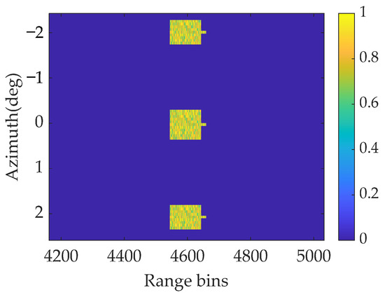
Figure 11.
Actual forward-looking image in surface target simulation.
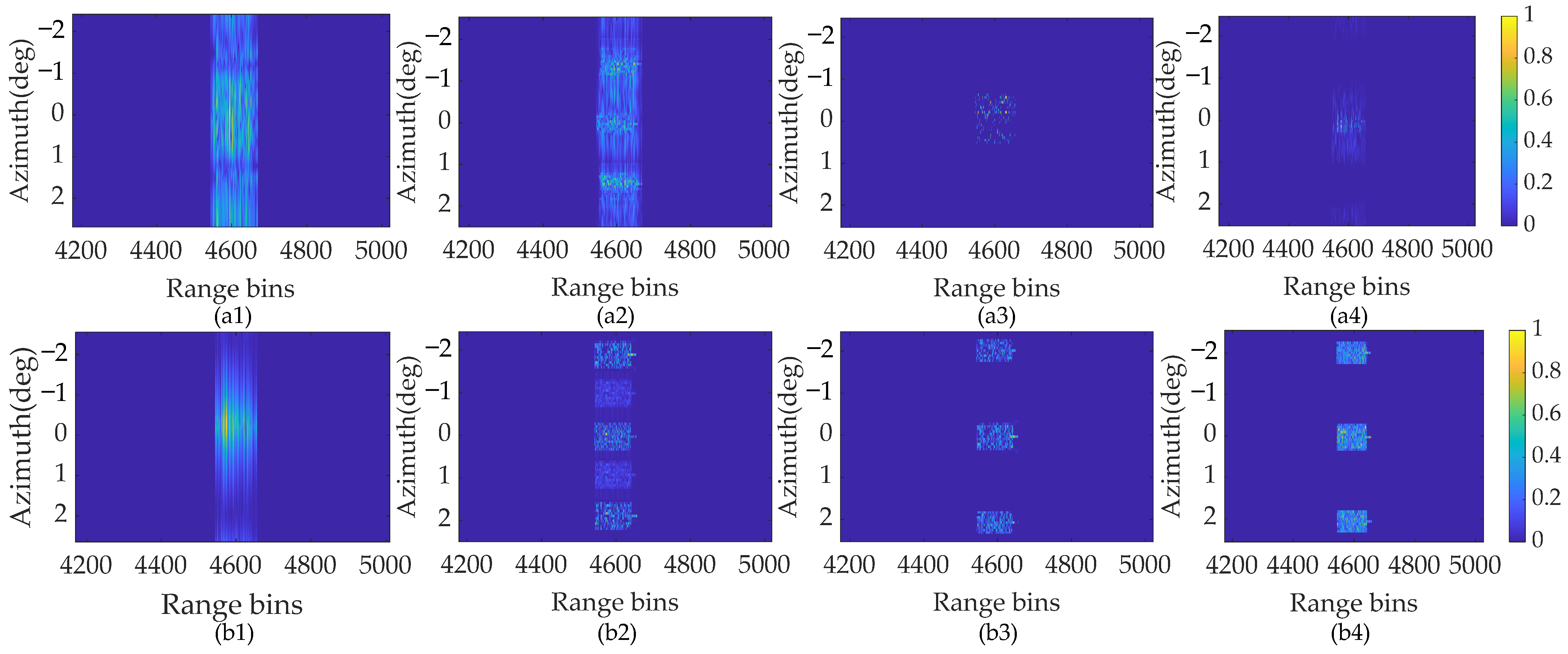
The reconstructed results using ISTA, SAMP, SBL, and the proposed SSTEM-VB methods are displayed in Figure 12. Figure 12(a1–a4) show the unsatisfactory results of the four super-resolution methods based on the conventional convolution model. This is because the high-order maneuverability causes the traditional dictionary to mismatch with the sparse scene reconstruction.
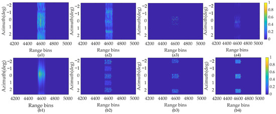
Figure 12.
Surface target super-resolution results with SNR of 18 dB. (a1) ISTA method. (a2) SAMP method. (a3) SBL method. (a4) SSTEM-VB method with conventional Doppler model. (b1) ISTA method. (b2) SAMP method. (b3) SBL method. (b4) SSTEM-VB method with proposed enhanced sparsity model.
In contrast, the sparse reconstruction results are optimized, as shown in Figure 12(b1–b4). In Figure 12(b1), the tank contour reconstructed with the ISTA method is blurred, resulting in coarse cross-range resolution. Higher performance is achieved with the SAMP and SBL methods compared with ISTA, as shown in Figure 12(b2,b3). However, several transverse ripples and non-negligible false targets appear in the reconstructed images using the SAMP method. Compared with the point target scene, it is evident from the surface target reconstructed results that, although the SBL method based on the traditional pixel sparse assumption can reconstruct the approximate outline, the internal structure of the target is discrete and missed. It significantly deteriorates the visual effect of the reconstruction. In comparison, the SSTEM-VB method restores the structural features, including clear contour and details, of the surface targets, and achieves a clustering effect, as shown in Figure 12(b4). Apparently, the SSTEM-VB method can produce well-focused forward-looking images, which is quite helpful to target recognition.
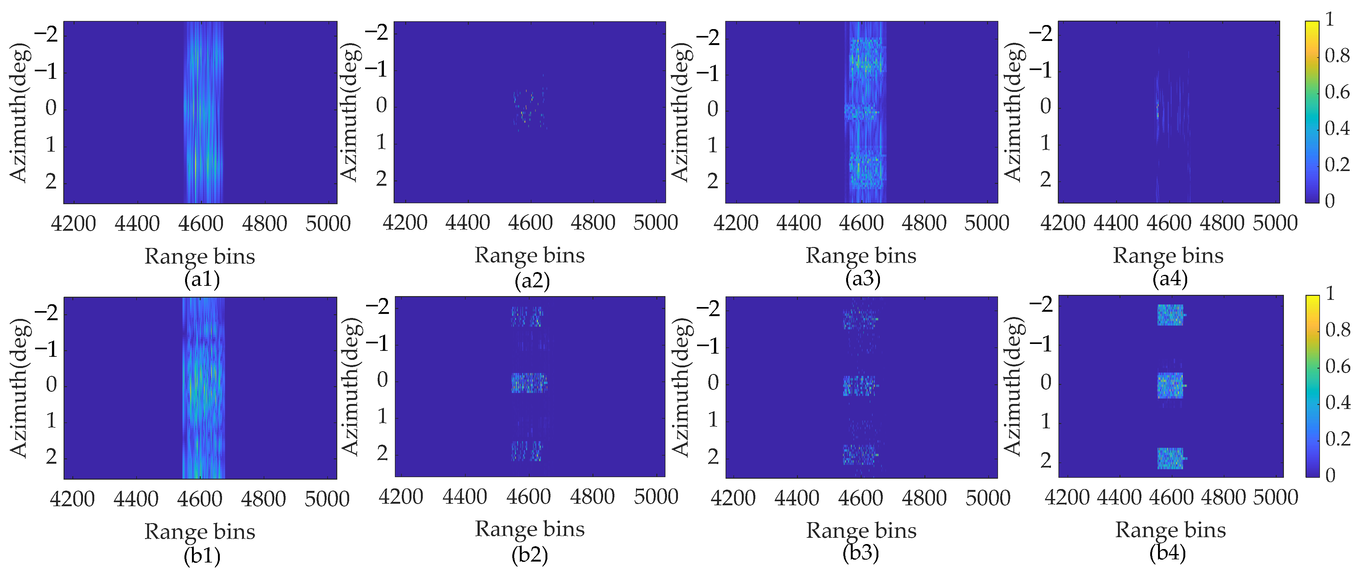
The performance using super-resulution imaging methods is greatly influenced by the deterioration of SNRs. The robustness of the algorithm in resolving ill-conditioned problems can be evaluated by the fluctuation in SNR. To demonstrate the robustness of the proposed algorithm with respect to SNR, simulated data with an SNR of 5 dB are processed. The super-resolution results under different processing models are shown in Figure 13.
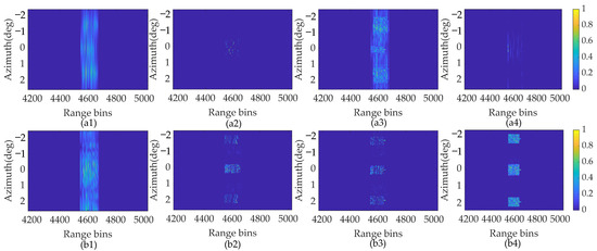
Figure 13.
Surface target super-resolution results with SNR of 5 dB. (a1) ISTA method. (a2) SAMP method. (a3) SBL method. (a4) SSTEM-VB method with conventional Doppler model. (b1) ISTA method. (b2) SAMP method. (b3) SBL method. (b4) SSTEM-VB method with proposed enhanced sparsity model.
Comparing Figure 12 and Figure 13, a similar conclusion can be obtained that the enhanced sparsity model performs better than the conventional model in super-resolution forward-looking imaging, regardless of the SNR levels. Inspecting Figure 13(b2,b3), the imaging results based on both SAMP and SBL methods further deteriorate when the SNR decreases to 5 dB. This phenomenon indicates that the pixel sparse assumption is not suitable for surface targets with block sparse features, causing loss of some detailed contour information and resulting in a more discrete image. On the contrary, the proposed SSTEM-VB method can maintain satisfactory recovery performance. Moreover, little deterioration is observed in the result from the proposed method under low SNR conditions. The contour of the block sparse targets is noticeably clearer in the result produced by the proposed method than the other algorithms.
In summary, observing the above processing results of simulated data, the SSTEM-VB method proposed in this paper, utilizing the enhanced sparsity model, is capable of achieving satisfactory super-resolution sparse recovery even under severe SNR conditions. It also significantly enhances the imaging quality of block sparse targets for maneuvering platforms.
5. Conclusions
In this article, we propose a super-resolution forward-looking imaging algorithm, SSTEM-VB, which utilizes the enhanced sparsity model for maneuvering trajectories. First, the imaging geometric model for maneuvering platform is established. Subsequently, the virtual MPCF is designed to correct the range walk and compensate for the high-order Doppler phase introduced by the maneuverability. Then, to enforce sparsity in the scene, the high-dimensional beam space is merged, and an optimized convolution model with enhanced sparsity is derived. Moreover, a structured hierarchical ST prior is exploited to model the sparse signal under the enhanced sparsity framework. It is more suitable for representing the sparseness of pattern-coupled scenes than traditional priors based on pixel sparse assumption. Eventually, an EM-based VB inference is applied to estimate the parameters of the sparse signal. The significant improvement in image performance achieved by the proposed method has been validated through numerical simulation results.
Author Contributions
Conceptualization, Y.G., Y.L. (Yujie Liang), and Y.L. (Yi Liang); methodology, Y.G.; software, Y.G.; validation, Y.G. and Y.L. (Yujie Liang); formal analysis, Y.L. (Yi Liang) and X.S.; resources, Y.L. (Yi Liang); writing—original draft preparation, Y.G.; writing—review and editing, Y.L. (Yujie Liang) and Y.L. (Yi Liang); visualization, Y.L. (Yujie Liang) and X.S.; supervision, Y.L. (Yujie Liang); funding acquisition, Y.L. (Yi Liang). All authors have read and agreed to the published version of the manuscript.
Funding
This work was supported by the National Natural Science Foundation of China under Grant 62271363.
Data Availability Statement
The raw data supporting the conclusions of this article will be made available by the authors on request.
Acknowledgments
We would like to thank the anonymous reviewers for their valuable comments to improve the paper quality.
Conflicts of Interest
Author Xiangwei Sun was employed by the company Xi’an LeiTong Science &Technology Co., Ltd. The remaining authors declare that the research was conducted in the absence of any commercial or financial relationships that could be construed as a potential conflict of interest.
References
- Xing, M.D.; Lin, H.; Chen, J.; Sun, G.; Yan, B. A review of imaging algorithms in multiplatform-borne synthetic aperture radar. J. Radars 2019, 8, 732–767. [Google Scholar]
- Sun, G.C.; Xing, M.; Xia, X.-G.; Wu, Y.; Bao, Z. Beam Steering SAR Data Processing by a Generalized PFA. IEEE Trans. Geosci. Remote Sens. 2013, 51, 4366–4377. [Google Scholar] [CrossRef]
- Long, T.; Lu, Z.; Ding, Z.; Liu, L. A DBS Doppler centroid estimation algorithm based on entropy minimization. IEEE Trans. Geosci. Remote Sens. 2011, 49, 3703–3712. [Google Scholar] [CrossRef]
- Chen, H.; Li, M.; Wang, Z.; Lu, Y.; Cao, R.; Zhang, P.; Zuo, L.; Wu, Y. Cross-range resolution enhancement for DBS imaging in a scan mode using aperture-extrapolated sparse representation. IEEE Geosci. Remote Sens. Lett. 2017, 14, 1459–1463. [Google Scholar] [CrossRef]
- Rocca, P.; Donelli, M.; Oliveri, G.; Viani, F.; Massa, A. Reconfigurable sum–difference pattern by means of parasitic elements for forward-looking monopulse radar. IET Radar Sonar Navig. 2013, 7, 747–754. [Google Scholar] [CrossRef]
- Chen, H.; Lu, Y.; Mu, H.; Yi, X.; Liu, J.; Wang, Z.; Li, M. Knowledge-aided mono-pulse forward-looking imaging for airborne radar by exploiting the antenna pattern information. Electron. Lett. 2017, 53, 566–568. [Google Scholar] [CrossRef]
- Qiu, X.; Hu, D.; Ding, C. Some reflections on bistatic SAR of forward-looking configuration. IEEE Geosci. Remote Sens. Lett. 2008, 5, 735–739. [Google Scholar] [CrossRef]
- Espeter, T.; Walterscheid, I.; Klare, J.; Brenner, A.R.; Ender, J.H.G. Bistatic forward-looking SAR: Results of a spaceborne–airborne experiment. IEEE Geosci. Remote Sens. Lett. 2011, 8, 765–768. [Google Scholar] [CrossRef]
- Meng, Z.; Li, Y.; Li, C.; Xing, M.; Bao, Z. A raw data simulator for bistatic forward-looking high-speed maneuvering-platform SAR. Signal Process. 2015, 117, 151–164. [Google Scholar] [CrossRef]
- Pu, W.; Wu, J.; Wang, X.; Huang, Y.; Zha, Y.; Yang, J. Joint sparsity-based imaging and motion error estimation for BFSAR. IEEE Trans. Geosci. Remote Sens. 2019, 57, 1393–1408. [Google Scholar] [CrossRef]
- Wu, J.; Li, Z.; Huang, Y.; Yang, J.; Yang, H.; Liu, Q.H. Focusing bistatic forward-looking SAR with stationary transmitter based on keystone transform and nonlinear chirp scaling. IEEE Geosci. Remote Sens. Lett. 2014, 11, 148–152. [Google Scholar] [CrossRef]
- Zhang, B.C.; Hong, W.; Wu, Y. Sparse microwave imaging: Principles and applications. Sci. China Inf. Sci. 2012, 55, 1722–1754. [Google Scholar] [CrossRef]
- Guan, J.C.; Yang, J.; Huang, Y.; Li, W. Maximum A Posteriori-Based Angular Super-Resolution for Scanning Radar Imaging. IEEE Trans. Aerosp. Electron. Syst. 2014, 50, 2389–2398. [Google Scholar] [CrossRef]
- Zha, Y.B.; Huang, Y.; Sun, Z.; Wang, Y.; Yang, J. Bayesian Deconvolution for Angular Super-Resolution in Forward-Looking Scanning Radar. Sensors 2015, 15, 6924–6946. [Google Scholar] [CrossRef] [PubMed]
- Zha, Y.B.; Huang, Y.; Sun, Z.; Wang, Y.; Yang, J. An Improved Richardson-Lucy Algorithm for Radar Angular Super-Resolution. In Proceedings of the 2014 IEEE Radar Conference, Cincinnati, OH, USA, 19–23 May 2014; pp. 406–410. [Google Scholar]
- Zhang, Y.C.; Mao, D.; Zhang, Q.; Zhang, Y.; Huang, Y.; Yang, J. Airborne Forward-Looking Radar Super-Resolution Imaging Using Iterative Adaptive Approach. IEEE J. Sel. Top. Appl. Earth Obs. Remote Sens. 2019, 12, 2044–2054. [Google Scholar] [CrossRef]
- Tropp, J.A.; Wright, S.J. Computational Methods for Sparse Solution of Linear Inverse Problems. Proc. IEEE 2010, 98, 948–958. [Google Scholar] [CrossRef]
- Dai, W.; Milenkovic, O. Subspace Pursuit for Compressive Sensing Signal Reconstruction. IEEE Trans. Inf. Theory 2009, 55, 2230–2249. [Google Scholar] [CrossRef]
- Zhang, Y. Theory and Method of Superresolution Imaging for Forward-Looking Radar of Moving Platform. Ph.D. Thesis, University of Electronic Science and Technology of China, Chengdu, China, 2016. [Google Scholar]
- Zhang, Y.; Li, W.; Zhang, Y.; Huang, Y.; Yang, J. A fast iterative adaptive approach for scanning radar angular superresolution. IEEE J. Sel. Top. Appl. Earth Observ. Remote Sens. 2015, 8, 5336–5345. [Google Scholar] [CrossRef]
- Chen, S.S.; Donoho, D.L.; Saunders, M.A. Atomic decomposition by basis pursuit. SIAM J. Sci. Comput. 1999, 20, 33–61. [Google Scholar] [CrossRef]
- Beck, A.; Teboulle, M. A Fast Iterative Shrinkgae-Thresholding Algorithm for Linear Inverse Problems. SIAM J. Imaging Sci. 2009, 2, 183–202. [Google Scholar] [CrossRef]
- Stoica, P.; Li, J.; He, H. Spectral analysis of nonuniformly sampled data: A new approach versus the periodogram. IEEE Trans. Signal Process. 2009, 57, 843–858. [Google Scholar] [CrossRef]
- Zhang, Y.; Zhang, Y.; Huang, Y.; Li, W.; Yang, J. Angular superresolution for scanning radar with improved regularized iterative adaptive approach. IEEE Geosci. Remote Sens. 2016, 13, 846–850. [Google Scholar] [CrossRef]
- Zhang, Y.; Zhang, Y.; Li, W.; Huang, Y.; Yang, J. Super-resolution surface mapping for scanning radar: Inverse filtering based on the fast iterative adaptive approach. IEEE Trans. Geosci. Remote Sens. 2018, 56, 127–144. [Google Scholar] [CrossRef]
- Zhang, Y.; Jakobsson, A.; Zhang, Y.; Huang, Y.; Yang, J. Wideband sparse reconstruction for scanning radar. IEEE Trans. Geosci. Remote Sens. 2018, 56, 6055–6068. [Google Scholar] [CrossRef]
- Zhang, Y.; Mao, D.; Yang, H.; Wu, J.; Huang, Y.; Yang, J. Online Sparse Reconstruction for scanning Radar Based on Generalized Sparse Iterative Covariance-Based Estimation. In Proceedings of the 2019 International Radar Conference (RadarConf2019), Toulon, France, 23–27 September 2019; pp. 1–4. [Google Scholar]
- Tropp, J.A.; Gilbert, A.C. Signal Recovery from Random Measurements via Orthogonal Matching Pursuit. IEEE Trans. Inf. Theory 2007, 53, 4655–4666. [Google Scholar] [CrossRef]
- Thong, T.D.; Gan, L.; Nguyen, N.; Tran, T.D. Sparsity Adaptive Matching Pursuit Algorithm for Practical Compressed Sensing. In Proceedings of the 2008 42nd Asilomar Conference on Signals, Systems and Computers, Paciffic Grove, CA, USA, 26–29 October 2008; pp. 581–587. [Google Scholar]
- Guo, Y.; Liang, Y.; Chen, D.; Suo, Z.; Li, S.; Xing, M. Superresolution Forward-Looking Imaging with Greedy Pursuit for High-speed Dynamic Platform Under Optimized Doppler Convolution Model. IEEE Trans. Geosci. Remote Sens. 2023, 61, 5108514. [Google Scholar] [CrossRef]
- Zhang, Y.; Zhang, Q.; Li, C.; Zhang, Y.; Huang, Y.; Yang, J. Seasurface target angular superresolution in forward-looking radar imaging based on maximum a posteriori algorithm. IEEE J. Sel. Top. Appl. Earth Observ. Remote Sens. 2019, 12, 2822–2834. [Google Scholar] [CrossRef]
- Yang, J.; Kang, Y.; Zhang, Y.; Huang, Y.; Zhang, Y. A Bayesian angular superresolution method with lognormal constraint for seasurface target. IEEE Access 2020, 8, 13419–13428. [Google Scholar] [CrossRef]
- Chen, H.; Li, Y.; Gao, W. Bayesian Forward-Looking Superresolution Imaging Using Doppler Deconvolution in Expanded Beam Space for High-Speed Platform. IEEE Trans. Geosci. Remote Sens. 2022, 60, 1–13. [Google Scholar] [CrossRef]
- Tzikas, D.G.; Likas, A.C.; Galatsanos, N.P. The variational approximation for Bayesian inference. IEEE Signal Process. Mag. 2008, 25, 131–146. [Google Scholar] [CrossRef]
- Li, W.; Li, M.; Zuo, L.; Chen, H.; Wu, Y.; Zhuo, Z. A Computationally Efficient Airborne Forward-Looking Super-Resolution Imaging Method Based on Sparse Bayesian Learning. IEEE Trans. Geosci. Remote Sens. 2023, 61, 5102613. [Google Scholar] [CrossRef]
- Ender, J.H.G. On Compressive Sensing Applied to Radar. Signal Process. 2010, 90, 1402–1414. [Google Scholar] [CrossRef]
- Bishop, C.M. Probability Distributions. In Pattern Recognition and Machine Learning; Springer Publications: Berlin, Germany, 2006; pp. 67–105. [Google Scholar]
- Wang, L.; Zhao, L.; Rahardja, S.; Bi, G. Alternative to extended block sparse Bayesian learning and its relation to pattern-coupled sparse Bayesian learning. IEEE Trans. Signal Process. 2018, 66, 2759–2771. [Google Scholar] [CrossRef]


Disclaimer/Publisher’s Note: The statements, opinions and data contained in all publications are solely those of the individual author(s) and contributor(s) and not of MDPI and/or the editor(s). MDPI and/or the editor(s) disclaim responsibility for any injury to people or property resulting from any ideas, methods, instructions or products referred to in the content. |
© 2025 by the authors. Licensee MDPI, Basel, Switzerland. This article is an open access article distributed under the terms and conditions of the Creative Commons Attribution (CC BY) license (https://creativecommons.org/licenses/by/4.0/).