
Correction Method for Thermal Deformation Line-of-Sight Errors of Low-Orbit Optical Payloads Under Unstable Illumination Conditions

Abstract
1. Introduction
- Variation in the angles of solar light incidence;
- Environmental temperature changes resulting from different distances between the camera and the sun;
- Thermal deformation caused by satellite launch processes.
- The angle relationship between the solar vector, satellite position vector, and camera LOS vector was innovatively utilized to characterize the thermal environment in which the payload operates. This provides the possibility of quantitatively analyzing the complex factors of the space thermal environment, overcoming the irregularity and frequent correction requirements of the LOS errors in low-orbit payloads.
- A LOS determination model for conversion from the pixel coordinates to celestial coordinates was established for low-orbit optical payloads, and potential errors introduced during the imaging process were analyzed.
- Neural networks were innovatively utilized in the correction of camera LOS issues, and the backpropagation neural network was used to solve the mapping relationship between the space thermal environment and camera LOS offset, which significantly enhanced the accuracy of the camera LOS correction.
2. Stellar-Based Determination Model of LOS
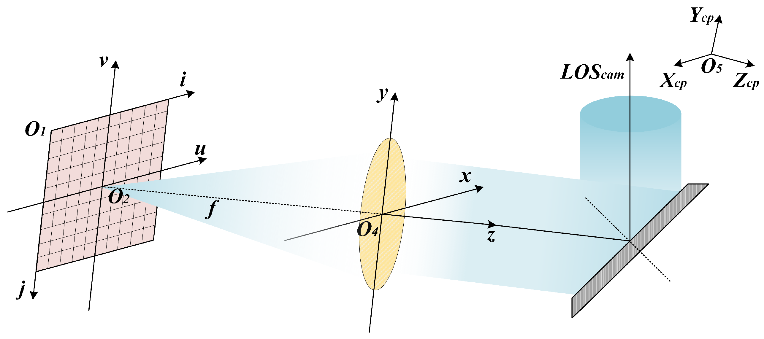
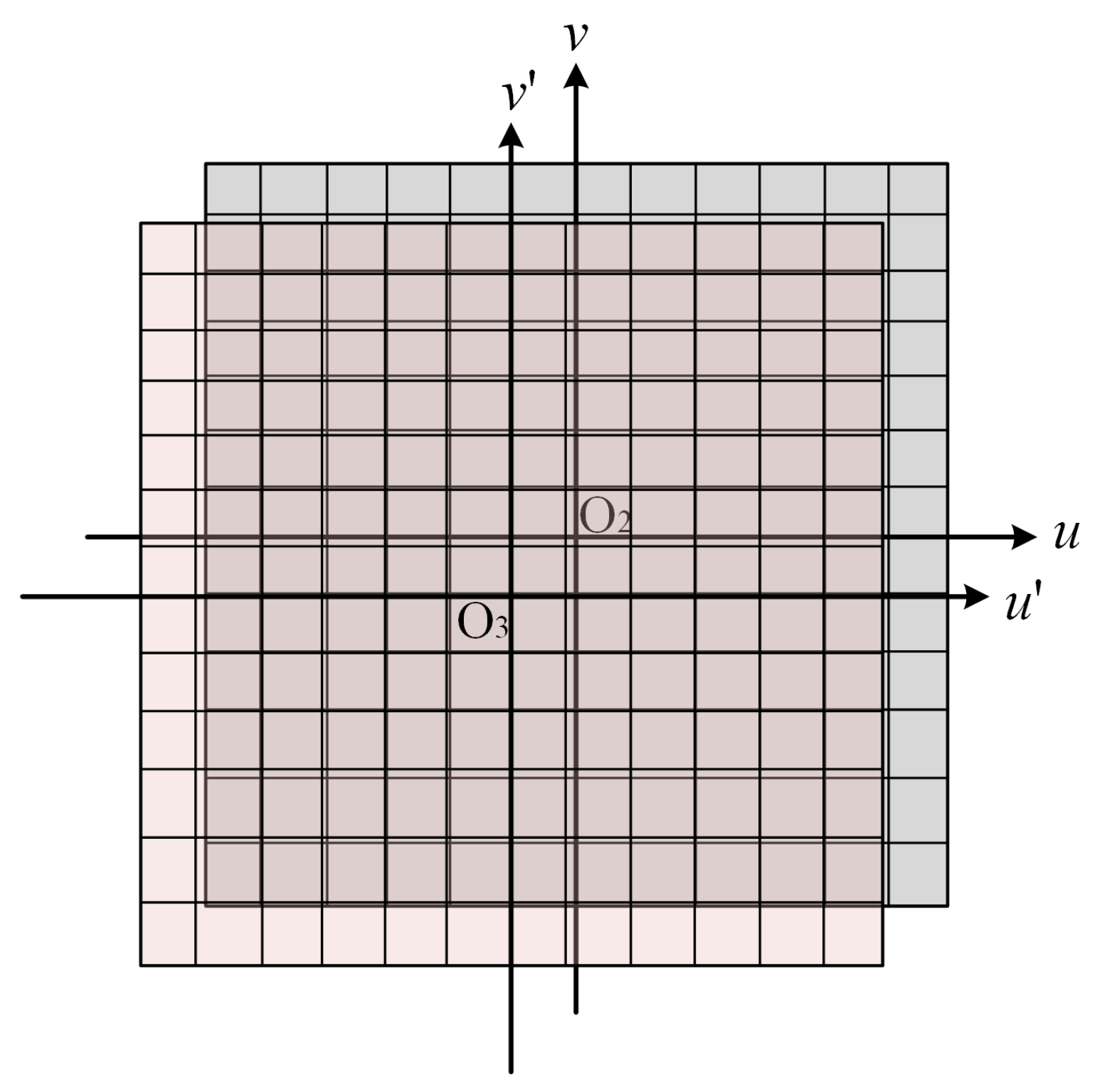
2.1. Interior Orientation Model
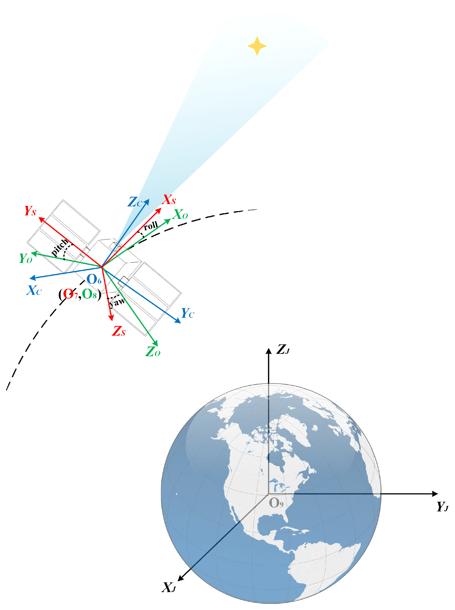
2.2. Exterior Orientation Model
2.3. Stellar-Based Imaging Model
- Measurement errors introduced during the measurement process of , , and ;
- Errors caused by STD and satellite platform vibrations;
- Changes in the distortion model of the camera after the on-orbit operation.
3. Correction Method for LOS
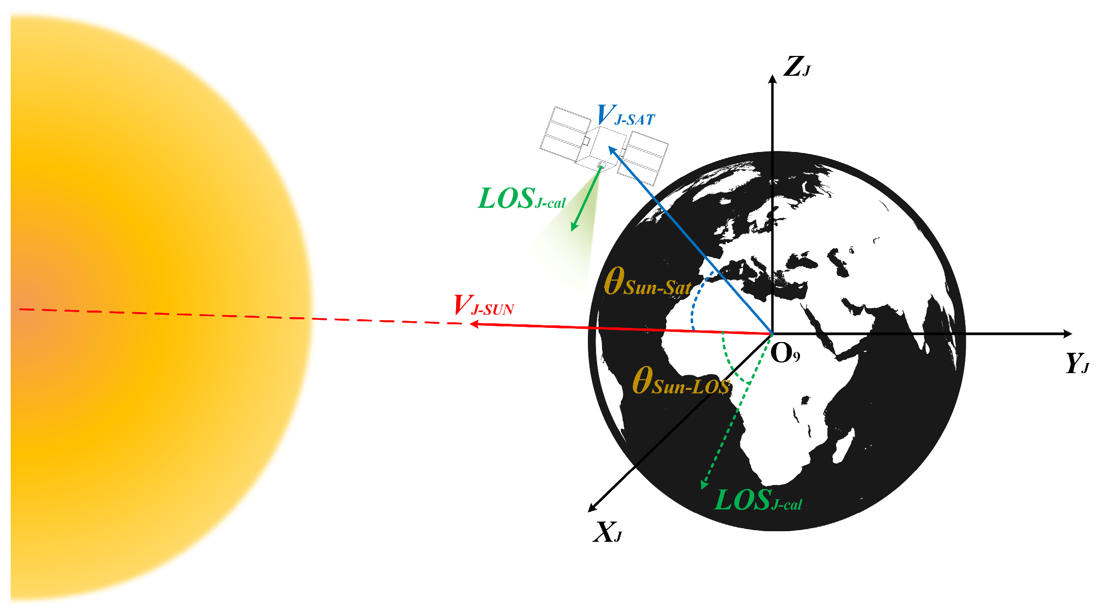
3.1. Analysis of Causes for LOS Error
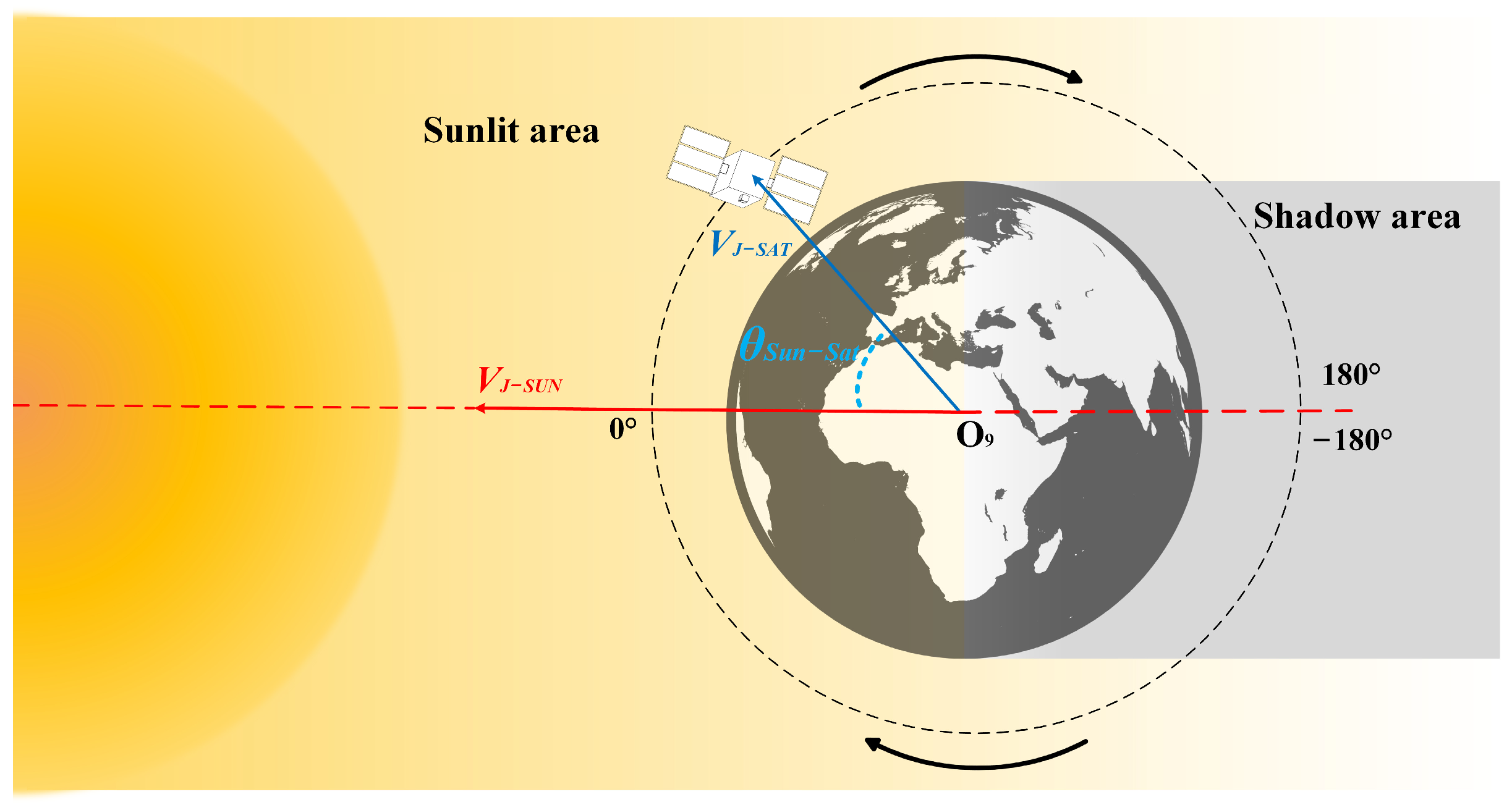
- : angle between the solar vector and the satellite position vector in the celestial coordinate system.
- : angle between the solar vector and the camera’s LOS vector in the celestial coordinate system.
3.1.1. Angle Between Solar Vector and Satellite Position Vector
- The satellite is flying from the shadow area to the sunlit area;
- The satellite is in the sunlit area but moving toward the shadow area.
3.1.2. Angle Between Solar Vector and Camera’s LOS Vector
3.2. Thermal Deformation Error Model
3.3. Correction Method
| Algorithm 1 NRBO-RIME-BP neural network |
|
|
|
|
|
|
|
|
|
|
|
4. Experimental Results
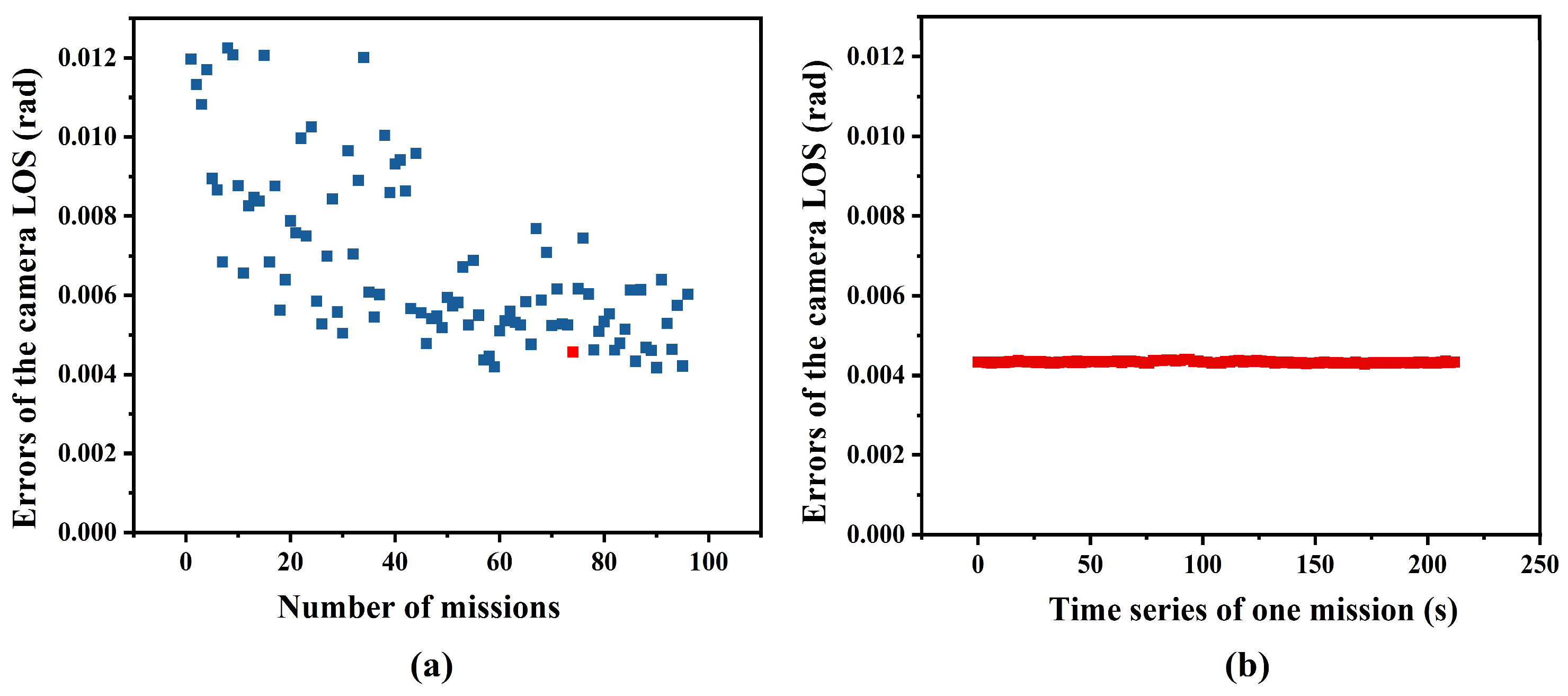
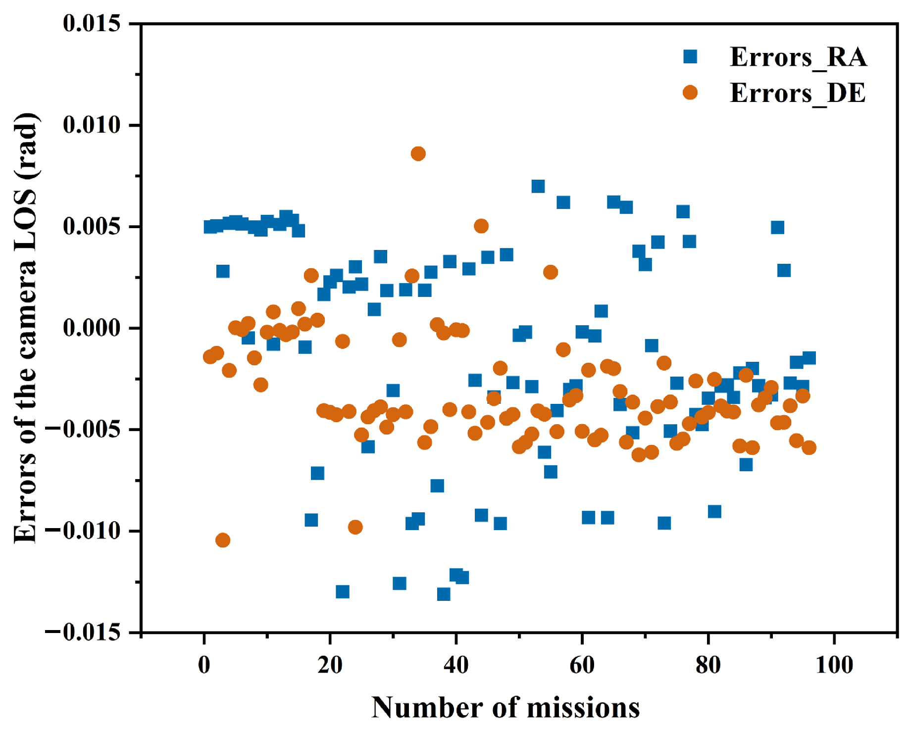
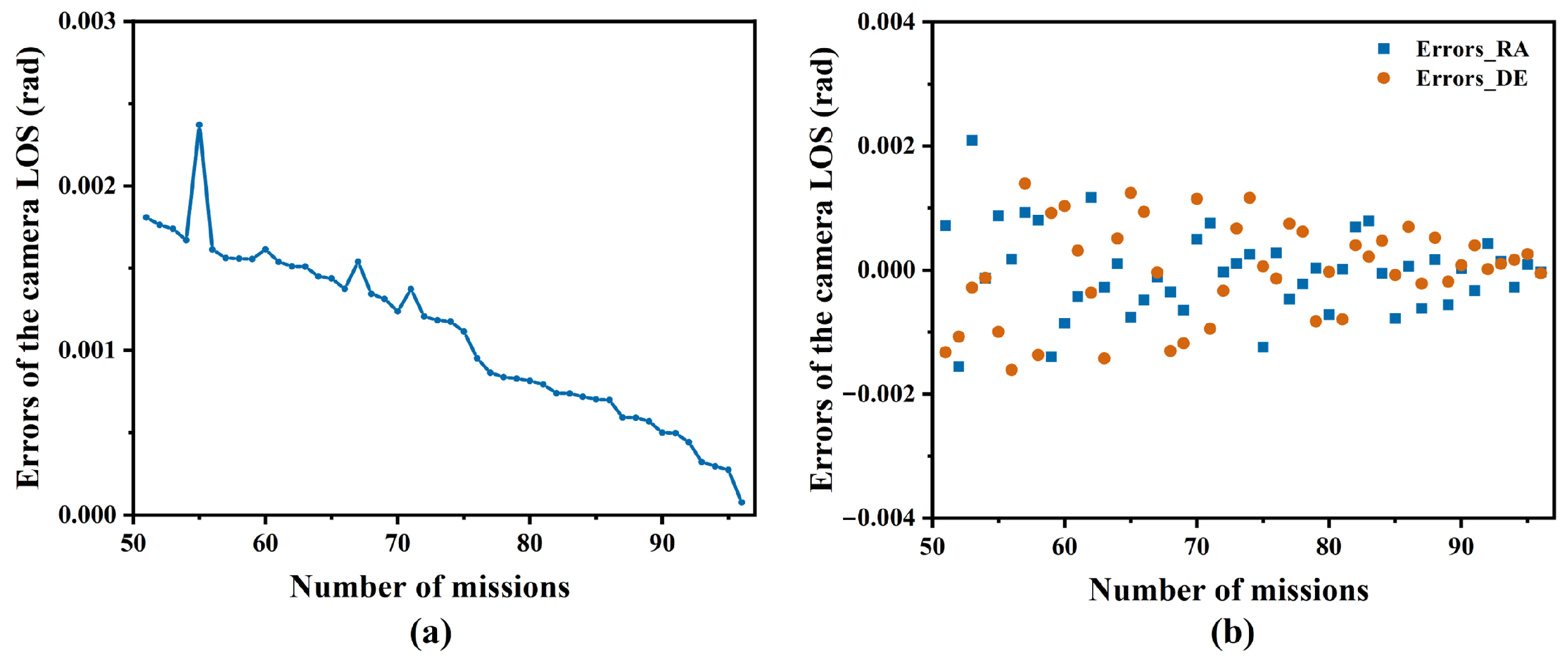
4.1. Variation Tendency Analysis of Camera LOS Error
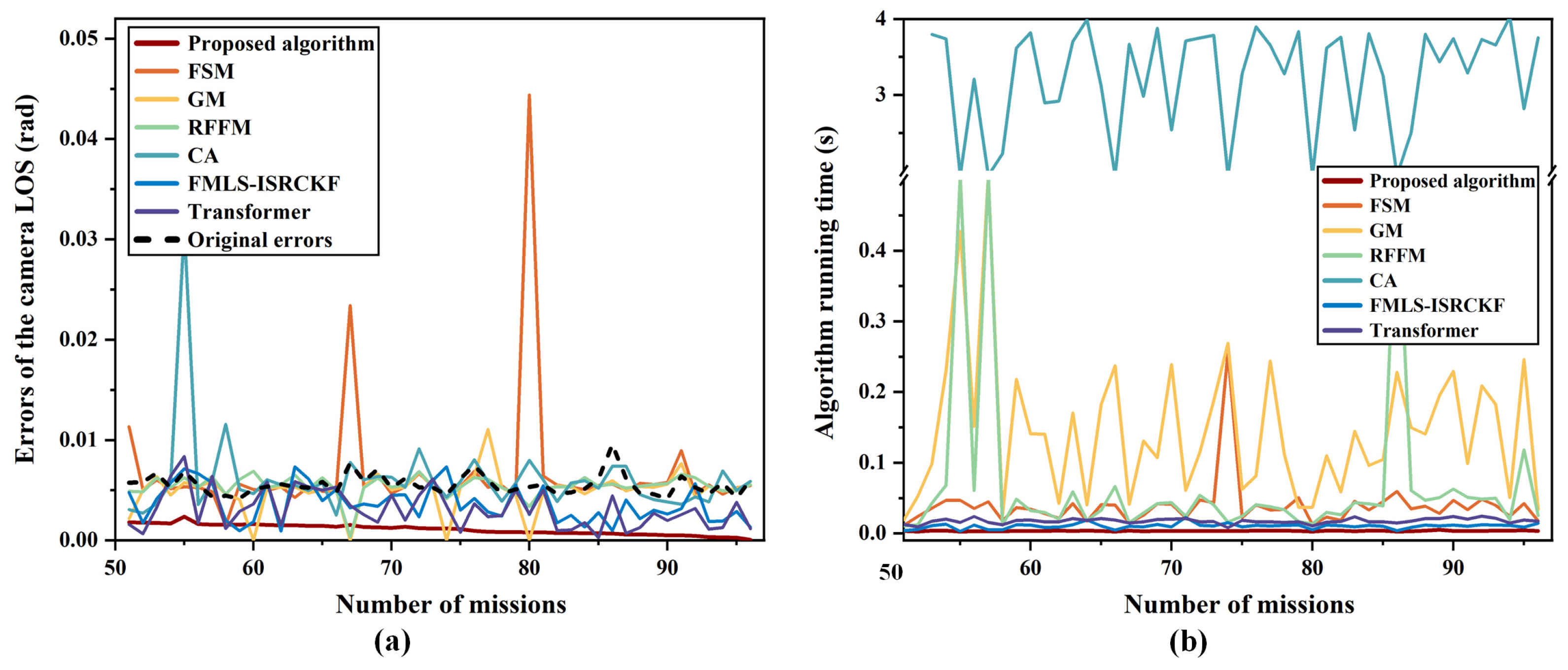
4.2. Correction Results of the Camera LOS
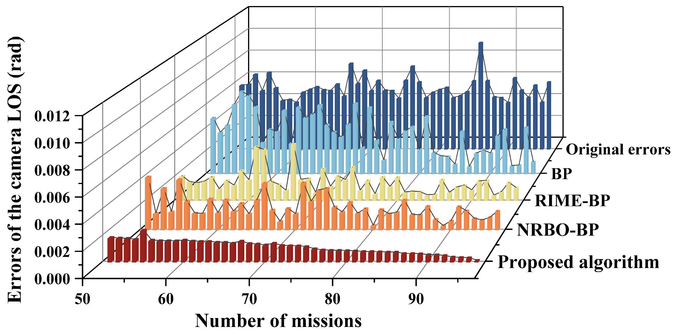
4.3. Results of the Ablation Experiment
4.4. Validation of the Extrapolation Ability of the Algorithm
5. Conclusions
Author Contributions
Funding
Data Availability Statement
Conflicts of Interest
Abbreviations
| LOS | Line of sight |
| STD | Space thermal deformation |
| EKF | Extended Kalman Filter |
| IOM | Interior orientation model |
| EOM | Exterior orientation model |
| NRBO | Newton–Raphson-Based Optimizer |
| TAO | Trap Avoidance Operator |
References
- Jia, J.; Wang, Y.; Zhuang, X.; Yao, Y.; Wang, S.; Zhao, D.; Shu, R.; Wang, J. High spatial resolution shortwave infrared imaging technology based on time delay and digital accumulation method. Infrared Phys. Technol. 2017, 81, 305–312. [Google Scholar] [CrossRef]
- Clemons, T.M., III; Chang, K.C. Effect of sensor bias on space-based bearing-only tracker. In Proceedings of the Signal Processing, Sensor Fusion, and Target Recognition XVII, Orlando, FL, USA, 17 April 2008; pp. 135–143. [Google Scholar]
- Clemons, T.M.; Chang, K.C. Bias correction using background stars for space-based IR tracking. In Proceedings of the 2009 12th International Conference on Information Fusion, Seattle, WA, USA, 6–9 July 2009; pp. 2028–2035. [Google Scholar]
- Li, X.; Yang, L.; Su, X.; Hu, Z.; Chen, F. A correction method for thermal deformation positioning error of geostationary optical payloads. IEEE Trans. Geosci. Remote Sens. 2019, 57, 7986–7994. [Google Scholar] [CrossRef]
- Li, J.; Tian, S.-F. An efficient method for measuring the internal parameters of optical cameras based on optical fibres. Sci. Rep. 2017, 7, 12479. [Google Scholar] [CrossRef] [PubMed]
- De Lussy, F.; Greslou, D.; Dechoz, C.; Amberg, V.; Delvit, J.M.; Lebegue, L.; Blanchet, G.; Fourest, S. Pleiades HR in flight geometrical calibration: Location and mapping of the focal plane. Int. Arch. Photogramm. Remote Sens. Spat. Inf. Sci. 2012, 39, 519–523. [Google Scholar] [CrossRef]
- Radhadevi, P.V.; Müller, R.; d‘Angelo, P.; Reinartz, P. In-flight geometric calibration and orientation of ALOS/PRISM imagery with a generic sensor model. Photogramm. Eng. Remote Sens. 2011, 77, 531–538. [Google Scholar] [CrossRef]
- Wu, A. SBIRS high payload LOS attitude determination and calibration. In Proceedings of the 1998 IEEE Aerospace Conference Proceedings (Cat. No.98TH8339), Snowmass, CO, USA, 28 March 1998; Volume 245, pp. 243–253. [Google Scholar]
- Chen, J.; An, W.; Deng, X.; Yang, J.; Sha, Z. Space based optical staring sensor LOS determination and calibration using GCPs observation. In Proceedings of the Electro-Optical and Infrared Systems: Technology and Applications XIII, Edinburgh, UK, 21 October 2016; pp. 327–334. [Google Scholar]
- Wang, M.; Cheng, Y.; Chang, X.; Jin, S.; Zhu, Y. On-orbit geometric calibration and geometric quality assessment for the high-resolution geostationary optical satellite GaoFen4. ISPRS J. Photogramm. Remote Sens. 2017, 125, 63–77. [Google Scholar] [CrossRef]
- Wang, M.; Cheng, Y.; Tian, Y.; He, L.; Wang, Y. A new on-orbit geometric self-calibration approach for the high-resolution geostationary optical satellite GaoFen4. IEEE J. Sel. Top. Appl. Earth Obs. Remote Sens. 2018, 11, 1670–1683. [Google Scholar] [CrossRef]
- Wu, A. Precision attitude determination for LEO spacecraft. In Proceedings of the Guidance, Navigation, and Control Conference, San Diego, CA, USA, 29–31 July 1996; p. 3753. [Google Scholar]
- Leprince, S.; Musé, P.; Avouac, J.-P. In-flight CCD distortion calibration for pushbroom satellites based on subpixel correlation. IEEE Trans. Geosci. Remote Sens. 2008, 46, 2675–2683. [Google Scholar] [CrossRef]
- Clemons, T.M.; Chang, K.-C. Sensor calibration using in-situ celestial observations to estimate bias in space-based missile tracking. IEEE Trans. Aerosp. Electron. Syst. 2012, 48, 1403–1427. [Google Scholar]
- Topan, H.; Maktav, D. Efficiency of orientation parameters on georeferencing accuracy of SPOT-5 HRG level-1A stereoimages. IEEE Trans. Geosci. Remote Sens. 2013, 52, 3683–3694. [Google Scholar] [CrossRef]
- Wang, M.; Zhu, Y.; Jin, S.; Pan, J.; Zhu, Q. Correction of ZY-3 image distortion caused by satellite jitter via virtual steady reimaging using attitude data. ISPRS J. Photogramm. Remote Sens. 2016, 119, 108–123. [Google Scholar] [CrossRef]
- Wang, T.; Zhang, G.; Li, D.; Tang, X.; Jiang, Y.; Pan, H.; Zhu, X.; Fang, C. Geometric accuracy validation for ZY-3 satellite imagery. ISPRS J. Photogramm. Remote Sens. 2013, 11, 1168–1171. [Google Scholar]
- Zhang, Y.; Zheng, M.; Xiong, J.; Lu, Y.; Xiong, X. On-orbit geometric calibration of ZY-3 three-line array imagery with multistrip data sets. IEEE Trans. Geosci. Remote Sens. 2013, 52, 224–234. [Google Scholar]
- Zhang, Y.; Zheng, M.; Xiong, X.; Xiong, J. Multistrip bundle block adjustment of ZY-3 satellite imagery by rigorous sensor model without ground control point. IEEE Geosci. Remote Sens. Lett. 2014, 12, 865–869. [Google Scholar]
- Guan, Z.; Zhang, G.; Jiang, Y.; Shen, X. Low-frequency attitude error compensation for the Jilin-1 satellite based on star observation. IEEE Trans. Geosci. Remote Sens. 2023, 61, 1–17. [Google Scholar]
- Chen, X.; Xing, F.; You, Z.; Zhong, X.; Qi, K. On-orbit high-accuracy geometric calibration for remote sensing camera based on star sources observation. IEEE Trans. Geosci. Remote Sens. 2021, 60, 1–11. [Google Scholar] [CrossRef]
- Liu, H.; Liu, C.; Xie, P.; Liu, S. Design of Exterior Orientation Parameters Variation Real-Time Monitoring System in Remote Sensing Cameras. Remote Sens. 2024, 16, 3936. [Google Scholar] [CrossRef]
- Huang, D.; Wang, Z.; Gong, J.; Ji, H. On-orbit attitude planning for Earth observation imaging with star-based geometric calibration. Sci. China Technol. Sc. 2025, 68, 1220602. [Google Scholar]
- Guan, Z.; Jiang, Y.; Zhang, G.; Zhong, X. Geometric Calibration for the Linear Array Camera Based on Star Observation. IEEE J. Sel. Top. Appl. Earth Obs. Remote Sens. 2024, 18, 368–384. [Google Scholar] [CrossRef]
- Sun, B.; Zhang, L.; Liu, H.; Xiao, Y.; Fan, G. Star sensor low-frequency error correction method based on identification and compensation of interior orientation elements. Measurement 2025, 246, 116746. [Google Scholar]
- Wang, Y.; Dong, Z.; Wang, M. Attitude Low-Frequency Error Spatiotemporal Compensation Method for VIMS Imagery of GaoFen-5B Satellite. IEEE Geosci. Remote Sens. Lett. 2024, 21, 1–5. [Google Scholar]
- Wang, M.; Yang, B.; Hu, F.; Zang, X. On-orbit geometric calibration model and its applications for high-resolution optical satellite imagery. Remote Sens. 2014, 6, 4391–4408. [Google Scholar] [CrossRef]
- Weng, J.; Cohen, P.; Herniou, M. Camera calibration with distortion models and accuracy evaluation. IEEE Trans. Pattern Anal. Mach. Intell. 1992, 14, 965–980. [Google Scholar]
- Wang, J.; Shi, F.; Zhang, J.; Liu, Y. A new calibration model of camera lens distortion. Pattern Recognit. 2008, 41, 607–615. [Google Scholar] [CrossRef]
- Salvi, J.; Armangué, X.; Batlle, J. A comparative review of camera calibrating methods with accuracy evaluation. Pattern Recognit. 2002, 35, 1617–1635. [Google Scholar] [CrossRef]
- Li, X.; Su, X.; Hu, Z.; Yang, L.; Zhang, L.; Chen, F. Improved distortion correction method and applications for large aperture infrared tracking cameras. Infrared Phys. Technol. 2019, 98, 82–88. [Google Scholar] [CrossRef]
- Zhang, Y.-J. Camera calibration. In 3-D Computer Vision: Principles, Algorithms and Applications; Springer: Berlin/Heidelberg, Germany, 2023; pp. 37–65. [Google Scholar]
- Yılmaztürk, F. Full-automatic self-calibration of color digital cameras using color targets. Opt. Express 2011, 19, 18164–18174. [Google Scholar] [CrossRef]
- Wang, Y.; Chen, F. Calibration of inner orientation elements and distort correction for large diameter space mapping camera. Editor. Off. Opt. Precis. Eng. 2016, 24, 675–681. [Google Scholar] [CrossRef]
- Zhao, G.; Liu, H.; Pei, Y. Distort Correction for Large Aperture Off-Axis Optical System. Chin. J. Lasers 2010, 37, 157. [Google Scholar]
- Wang, M.; Cheng, Y.; Yang, B.; Jin, S.; Su, H. On-orbit calibration approach for optical navigation camera in deep space exploration. Opt. Express 2016, 24, 5536–5554. [Google Scholar] [CrossRef]
- Jiang, L.; Li, X.; Li, L.; Yang, L.; Yang, L.; Hu, Z.; Chen, F. On-orbit geometric calibration from the relative motion of stars for geostationary cameras. Sensors 2021, 21, 6668. [Google Scholar] [CrossRef] [PubMed]
- Jiang, F.; Wang, L.; Deng, H.; Zhu, L.; Kong, D.; Guan, H.; Liu, J.; Wang, Z. Thermal Deformation Analysis of a Star Camera to Ensure Its High Attitude Measurement Accuracy in Orbit. Remote Sens. 2024, 16, 4567. [Google Scholar] [CrossRef]
- Xia, H.; Tang, X.; Mo, F.; Xie, J.; Li, X. Geographically-Informed Modeling and Analysis of Platform Attitude Jitter in GF-7 Sub-Meter Stereo Mapping Satellite. ISPRS Int. J. Geo-Inf. 2024, 13, 413. [Google Scholar] [CrossRef]
- Meeus, J.H. Astronomical Algorithms; Willmann-Bell, Incorporated: Richmond, VA, USA, 1991. [Google Scholar]
- Li, C.; He, J.; Li, M.; Lai, P. Overview of research on Satellite shadow model and calculation methods. Sci. Technol. Innov. 2021, 11, 5–8. [Google Scholar] [CrossRef]
- Neta, B.; Vallado, D. On satellite umbra/penumbra entry and exit positions. J. Astronaut. Sci. 1998, 46, 91–103. [Google Scholar] [CrossRef]
- Sowmya, R.; Premkumar, M.; Jangir, P. Newton-Raphson-based optimizer: A new population-based metaheuristic algorithm for continuous optimization problems. Eng. Appl. Artif. Intell. 2024, 128, 107532. [Google Scholar]
- Su, H.; Zhao, D.; Heidari, A.A.; Liu, L.; Zhang, X.; Mafarja, M.; Chen, H. RIME: A physics-based optimization. Neurocomputing 2023, 532, 183–214. [Google Scholar]
- Vaswani, A.; Shazeer, N.; Parmar, N.; Uszkoreit, J.; Jones, L.; Gomez, A.N.; Kaiser, Ł.; Polosukhin, I. Attention is all you need. In Proceedings of the Advances in Neural Information Processing Systems 30 (NIPS 2017), Long Beach, CA, USA, 4–9 December 2017; Volume 30. [Google Scholar]


| Items | Detailed Parameters |
|---|---|
| Orbit altitude (H) | 7.19 × 10⁵ m |
| Orbital period (T) | 100 min |
| Camera type | Space observation camera |
| Pixel size () | 30 μm |
| Detector size (S) | 512 × 512 pixels |
| Focal distance () | 1430 mm |
| Field of view (F) | 1.1° × 1.1° |
| Method | Mean Error (rad) | Algorithm Speed (s/One Data Point) |
|---|---|---|
| Proposed algorithm | 0.001096 | 0.000016 |
| FSM | 0.006704 | 0.000201 |
| GM | 0.004937 | 0.000981 |
| RFFM | 0.005415 | 0.001014 |
| CA | 0.006078 | 0.010598 |
| FMLS-ISRCKF | 0.003673 | 0.000045 |
| Transformer | 0.003124 | 0.000082 |
| Original errors | 0.005559 | / |
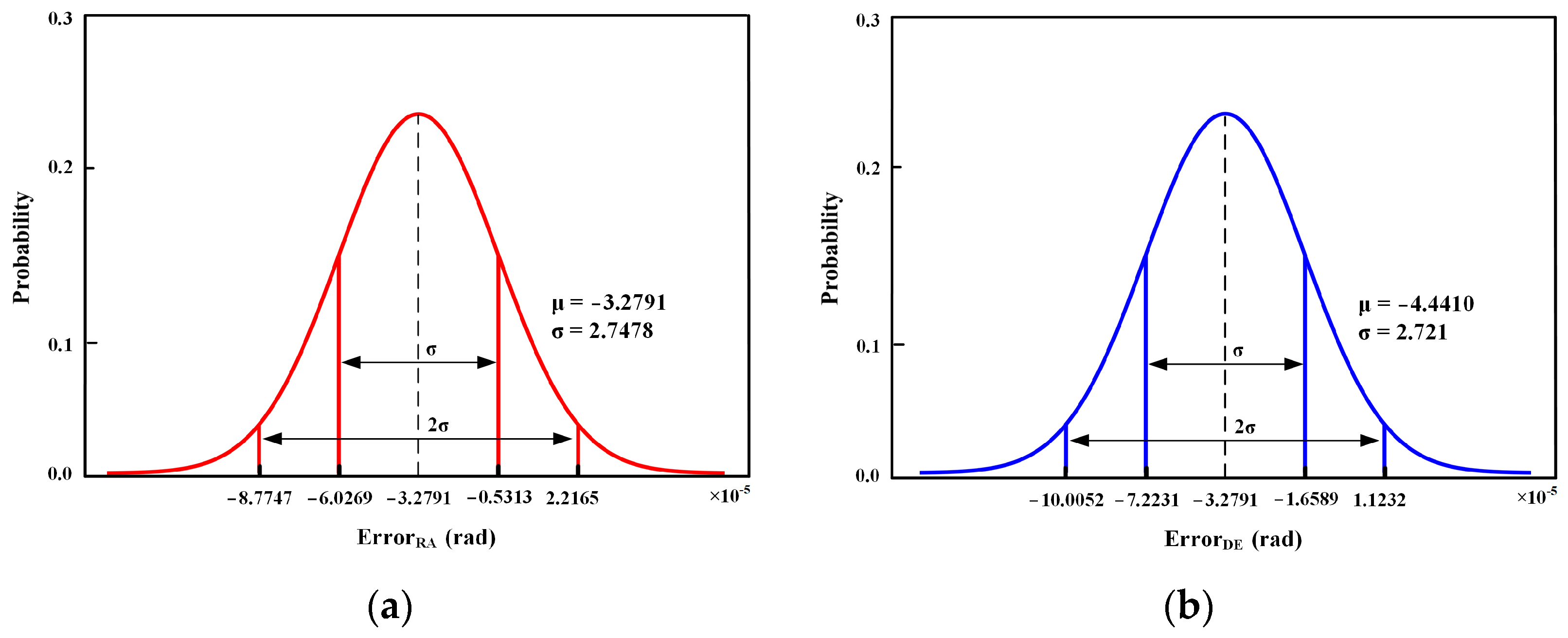
| CL * | 95% | |
| (×10−5) | −3.2791 | −4.4410 |
| CI of (×10−5) | (−3.6729, −2.8853) | (−4.8348, −4.0472) |
| (×10−5) | 2.7478 | 2.7821 |
| CI of (×10−5) | (2.4947, 3.0585) | (2.5102, 3.0776) |
| Test Set Data | Corresponding Training Set Data | |
|---|---|---|
| Mission number | 49 | 89 |
| Time of mission | 16 July 2023 16:33–16:38 | 21 November 2023 10:25–10:30 |
| The mean value of /° | 106.69 | 101.75 |
| The mean value of /° | 89.34 | 92.44 |
| Mission number | 10 | 3 |
| Time of mission | 21 June 2023 4:57–4:62 | 18 June 2023 4:46–4:50 |
| The mean value of /° | 152.67 | 154.26 |
| The mean value of /° | 160.09 | 162.91 |
Disclaimer/Publisher’s Note: The statements, opinions and data contained in all publications are solely those of the individual author(s) and contributor(s) and not of MDPI and/or the editor(s). MDPI and/or the editor(s) disclaim responsibility for any injury to people or property resulting from any ideas, methods, instructions or products referred to in the content. |
© 2025 by the authors. Licensee MDPI, Basel, Switzerland. This article is an open access article distributed under the terms and conditions of the Creative Commons Attribution (CC BY) license (https://creativecommons.org/licenses/by/4.0/).
Share and Cite
Li, Y.; Chen, X.; Liu, G.; Rao, P. Correction Method for Thermal Deformation Line-of-Sight Errors of Low-Orbit Optical Payloads Under Unstable Illumination Conditions. Remote Sens. 2025, 17, 762. https://doi.org/10.3390/rs17050762
Li Y, Chen X, Liu G, Rao P. Correction Method for Thermal Deformation Line-of-Sight Errors of Low-Orbit Optical Payloads Under Unstable Illumination Conditions. Remote Sensing. 2025; 17(5):762. https://doi.org/10.3390/rs17050762
Chicago/Turabian StyleLi, Yao, Xin Chen, Guangsen Liu, and Peng Rao. 2025. "Correction Method for Thermal Deformation Line-of-Sight Errors of Low-Orbit Optical Payloads Under Unstable Illumination Conditions" Remote Sensing 17, no. 5: 762. https://doi.org/10.3390/rs17050762
APA StyleLi, Y., Chen, X., Liu, G., & Rao, P. (2025). Correction Method for Thermal Deformation Line-of-Sight Errors of Low-Orbit Optical Payloads Under Unstable Illumination Conditions. Remote Sensing, 17(5), 762. https://doi.org/10.3390/rs17050762