A Novel Method for Denoising Lunar Satellite Gravity Anomaly Data Based on Prior Knowledge Deep Learning

Abstract

High-resolution lunar gravity anomaly data are of great significance for the study of the lunar crust and lithosphere structure, asymmetric thermal evolution, impact basin subsurface structure and mass tumor genesis, breccia, and magmatism. However, due to errors in satellite orbit and instrument observation, correlation error in high-order spherical harmonic coefficients, and other factors, satellite observation gravity anomaly data present evident aliasing phenomena of stripe noise and random noise in the spatial domain, resulting in difficulties in practical application analysis. In this paper, a lunar satellite gravity anomaly denoising method based on prior knowledge deep learning is proposed. In one instance, the prior knowledge is fused into the data set, the manual processing results are labeled, and the six label-superimposed directions of the simulated stripe noise are used as the sample input data. Conversely, because the gravity field is a harmonic field with smooth characteristics, the Laplace constraint is added to the loss function, and the deep learning results are optimized through Gaussian filtering. Synthetic and real data tests demonstrate the effectiveness of the proposed method in removing complex noise from lunar satellite gravity anomaly data.

1. Introduction

High-resolution lunar gravity anomaly data from the Gravity Recovery and Interior Laboratory (GRAIL) can be used to study lunar crust and lithosphere structure, asymmetric thermal evolution, impact basin underground structure and mass tumor genesis, breccia, and magmatism [1,2,3]. However, due to errors in satellite orbit and instrument observation, correlation error in high-order spherical harmonic coefficients, and other factors, gravity anomaly data observed by satellites present the evident aliasing phenomena of stripe noise and random noise in the spatial domain [4,5], resulting in difficulties in practical application analysis. Therefore, research on denoising lunar gravity anomaly data holds significant scientific importance and has practical implications.

Traditional satellite gravity anomaly data denoising methods include Gaussian filter (GF) [6], sliding polynomial fitting [4], the decorrelation method [7], and combination filtering of different methods. The main principle of these methods is to achieve noise removal by reducing the coefficient weight of higher-order terms of the model or eliminating the correlation error between the parity and even terms of the spherical harmonic coefficients. However, the selection of these filtering methods and filtering parameters requires a certain level of experience and the processing procedure is relatively complicated. The omnidirectional filtering (ODF) method [5] is a new method specifically aimed at removing stripe noise and random noise from lunar gravity anomaly data. This method simulates lunar noise in conditions close to reality. Through a set of user-defined azimuth parameters, it effectively eliminates multi-directional aliasing stripe noise; however, the window size must be adjusted through manual trial and error to balance strip removal and effective signal retention.

In recent years, deep learning has developed extensively in the field of geophysics [8,9] and has been widely applied to seismology [10], electromagnetism [11], gravitation [12], magnetometry [13], and other sub-disciplines. From data processing [14,15] and forward inversion [16,17,18,19] to geological interpretation [20,21] and other complete processes, a series of innovative achievements have been noted. In particular, in the application of deep learning for denoising geophysical data, a multitude of innovative research results have been published. These results relate to works primarily utilizing deep residual networks [22,23,24], convolutional neural networks [15,25,26,27], self-attention neural networks [28,29], convolutional autoencoders [30,31], and multi-layer perceptron networks [32]. Despite these achievements, there are still few studies on stripe noise removal. A convolutional neural network [26] was first applied to remove the stripe noise of airborne magnetic data along the measurement line, and excellent results were achieved in both synthetic and real data. A deep-learning-based method [28], which combines a self-attention neural network with convolutional self-encoding, can accurately identify and remove single-directional stripe interference and Gaussian-distributed noise. Nevertheless, applying existing methods directly to lunar gravity anomaly data denoising is challenging due to the superposition of multi-directional stripe noise and random noise.

In fact, deep learning has an earlier and more extensive application in processing stripe noise in optical images. The SNRCNN is used for stripe noise removal in single-band infrared images [33], the ICSRN model realizes stripe noise removal on infrared cloud images [34], and the HSI-DeNet can cope with various types of noise in each channel in hyperspectral images [35]. Since satellite gravity anomaly data can also be regarded as images, the above methods and concepts can be used for reference in the denoising application of satellite gravity anomaly data.

Based on the aforementioned analysis, we employed deep learning techniques in the following study to denoise lunar satellite gravity anomaly data. In this study, a six-layer U-Net deep learning network was built, which fuses the manually extracted useful signals of gravity field and the understanding of noise into the data set as prior knowledge, takes the results of manual denoising processing as labels, and takes the label superimposed analog stripe noise of six directions as sample input data. Because the gravity field is a harmonic field with smooth characteristics, a Laplacian constraint is added to the loss function, and the deep learning results are optimized via Gaussian filtering. Synthetic and real data tests demonstrate the effectiveness of the proposed method in removing the banding noise of lunar satellite gravity anomaly data.

2. Materials and Methods

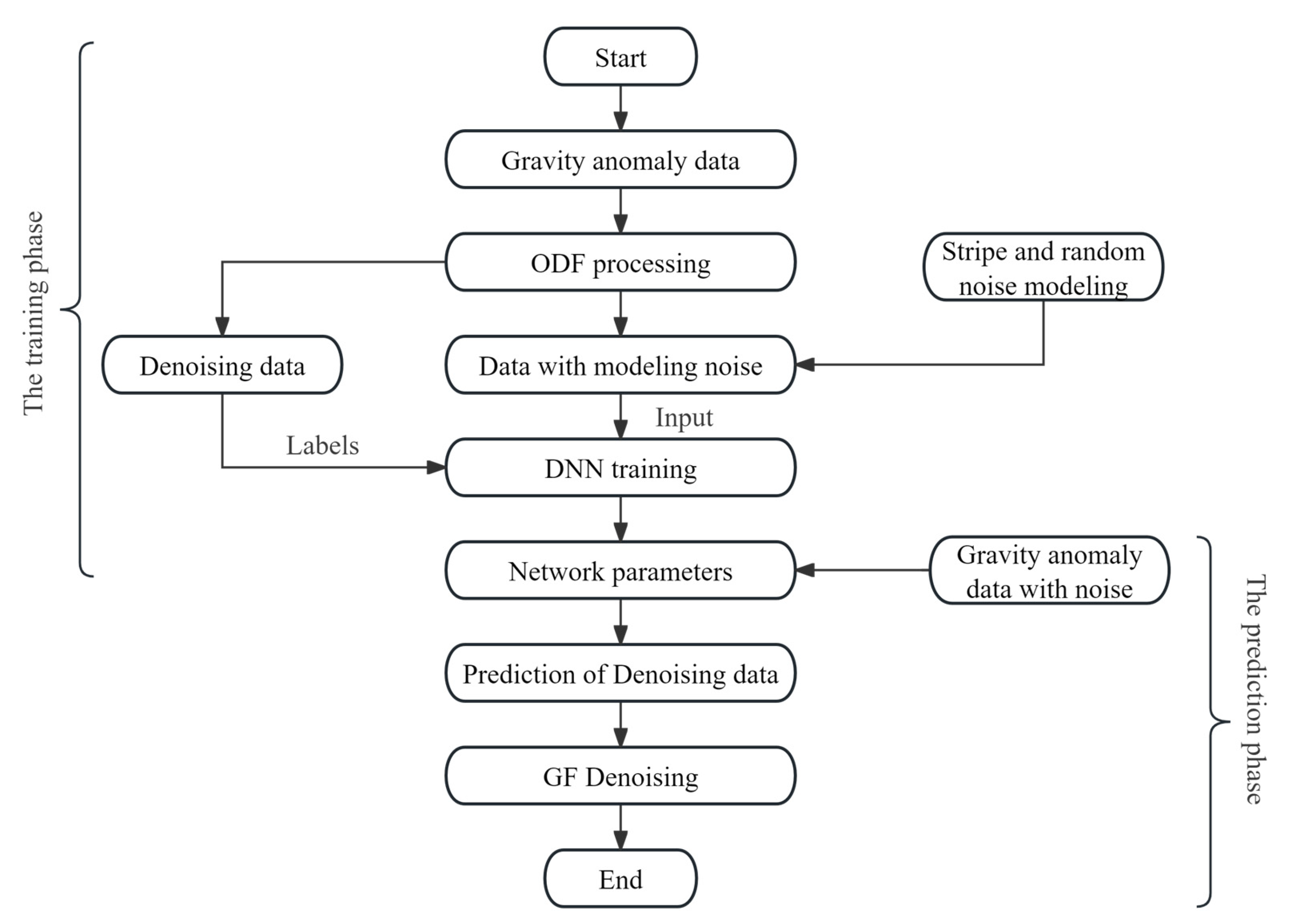
In this study, we adopt the supervised deep learning method, with the data processing workflow shown in Figure 1. In the training data set stage, first, noiseless lunar gravity anomaly data are constructed as output labels, which are the results of denoising using the ODF method [5]; that is, the labels contain prior knowledge of useful signals around the lunar gravity field. Subsequently, the sum of the lunar gravity noise generated by the label and the simulation is used as the input data of the deep neural network, that is, the input data contain the artificial empirical knowledge of the noise. On this basis, the optimal neural network parameters are obtained by fine-tuning the hyperparameters to train the deep learning network. In the prediction stage, the trained network is used to predict the lunar gravity anomaly data containing noise and the denoised lunar gravity anomaly data are obtained. According to the smoothing property of the gravity field as a harmonic field, the deep learning prediction results are optimized using the traditional low-pass filtering method to obtain the final result. The key to the above process is to develop a sufficient number of noisy lunar satellite gravity anomaly data sets with high accuracy, so as to comprehensively and objectively reflect the complexity of the original lunar satellite gravity anomaly noise and characteristics.

2.1. Deep Learning Architecture

We aim to solve the problem of denoising the original lunar satellite gravity anomaly data through deep learning technology. The core is to build a complex mapping relationship between noisy data and non-noisy data by learning a large amount of data. This mapping relationship can be expressed as follows:

$${\mathbf{d}}_{\mathbf{2}}= \mathrm{Net}({\mathbf{d}}_1,\mathbf{\theta })$$

(1)

where ${\mathbf{d}}_1$ and ${\mathbf{d}}_2$ represent the input data and output data of the deep learning network, respectively, and $\mathbf{\theta }$ is the deep learning network parameters.

As shown in Figure 2, we designed a deep learning network based on U-Net architecture [36] for denoising the original satellite gravity anomaly data. The deep learning network designed in this paper has a total structure of 6 layers, consisting of 25 2D convolution layers (kernel size 3 × 3, step size 1), 5 downsampling layers (kernel size 2 × 2, step size 2), 5 upsampling layers (kernel size 2 × 2, step size 2), and 5 skip connections. The numbers shown in red indicate the size of the data grid, and black numbers indicate the number of channels. The resolution of the input data and the output data is 160 × 160, and the resolution of the data in layers 2 to 6 is 80 × 80, 40 × 40, 20 × 20, 10 × 10, and 5 × 5, respectively. The number of contrary channels is doubled from 64 in layer 1 to 2048 in layer 6. Among them, the two-dimensional convolution layer and the lower sampling layer are both composed of a two-dimensional convolution operator, a batch normalization operator, and a Leaky-ReLU activation function, and the upper sampling layer is realized by two-dimensional transposed convolution.

During network training, input data enter the network from the upper left corner of Figure 2, and the feature information of this layer scale is extracted through two successive convolution operations of the first layer. Thereafter, a downsampling operation is performed to halve the resolution of the data and retain the feature information obtained by the upper layer. The above operations are repeated until the last layer, in the process of continuously increasing the receptive field, gradually realizing the feature extraction from the local information of the input data to the global information. Next, we enter the upsampling operation on the right side, recover the resolution of the data layer by layer, and realize the information fusion with the left side of the same resolution feature through the jump connection. Lastly, five two-dimensional convolution layers are applied to the output end of the network to obtain the denoising results of the noisy data.

2.2. Loss Function

In deep learning, the loss function serves a pivotal role as a non-negative real-valued function that quantifies the discrepancy between the models’ predicted output and the actual target value. The Dice function [37] focuses on the overlap between the predicted result and the real label, which can better retain the details and structure of the image. In this paper, this function is introduced into the denoising of gravity data to represent the similarity or overlap between the denoised data and the original data. When the Dice function is 1, this means that the denoised data and the original data completely overlap. Therefore, the Dice loss function is constructed as follows:

$$\mathrm{Dice}\mathrm{Loss} ={\displaystyle \frac{1}{N}}{\displaystyle {\sum }_{i=1}^N(1-\frac{{\displaystyle {\sum }_j^M{\widehat{\mathbf{d}}}_j^i{\mathbf{d}}_j^i}}{{{\displaystyle {\sum }_j^M{\widehat{\mathbf{d}}}_j^i}}^2+{\displaystyle {\sum }_j^M{{\mathbf{d}}_j^i}^2}})}$$

(2)

where $\widehat{\mathbf{d}}$ and $\mathbf{d}$ are the predicted value of gravity data denoising and the value of gravity data denoising, respectively, $N$ is the number of training samples, and $M$ represents the number of grid points for each sample.

The Dice loss function can restrict the similarity between the denoised data and the original data, yet it is difficult to achieve a smooth transition between adjacent data. However, the Bouguer gravity anomaly caused by underground geologic bodies has smooth characteristics on the plane; therefore, the Laplacian operator [38,39] is introduced to restrict the smoothness of the predicted results. The Laplacian operator can be expressed as the sum of the two-dimensional partial derivatives of the denoising predicted value of gravity data $\widehat{\mathbf{d}}$ on a two-dimensional grid with respect to the $x$ direction and y direction, respectively:

$${\Delta }^2\widehat{\mathbf{d}}={\displaystyle \frac{\partial {\widehat{\mathbf{d}}}^2}{\partial x^2}}+{\displaystyle \frac{\partial {\widehat{\mathbf{d}}}^2}{\partial y^2}}$$

(3)

Thus, the Laplace loss can be expressed as the following discrete form:

$$\begin{array}{l}\mathrm{Laplacian} \mathrm{loss}={\Delta }^2\widehat{\mathbf{d}} \approx \widehat{\mathbf{d}} (x,y-1)+\widehat{\mathbf{d}} (x,y+1)\\ +\widehat{\mathbf{d}} (x-1,y)+\widehat{\mathbf{d}} (x+1,y) - 4\widehat{\mathbf{d}} (x,y)\end{array}$$

(4)

Therefore, the total loss function can be expressed as:

$$\mathrm{Total} \mathrm{Loss} ={\displaystyle \frac{1}{N}}{\displaystyle {\sum }_{i=1}^N(1-\frac{{\displaystyle {\sum }_j^M{\widehat{\mathbf{d}}}_j^i{\mathbf{d}}_j^i}}{{{\displaystyle {\sum }_j^M{\widehat{\mathbf{d}}}_j^i}}^2+{\displaystyle {\sum }_j^M{{\mathbf{d}}_j^i}^2}})}+\lambda {\Delta }^2\widehat{\mathbf{d}}$$

(5)

where $\lambda$ is the weight coefficient, which is used to adjust the proportion between Dice loss and Laplace loss.

2.3. Deep Learning Results Optimization

The denoising results of synthetic data show that the predicted value of gravity data denoising constrained by Dice loss and Laplace loss still has a small amount of high-frequency noise. Therefore, Gaussian filtering is introduced to perform low-pass filtering on the deep learning prediction results to obtain the final denoising result of gravity data, in which the Gaussian kernel is adopted as follows:

$$\mathbf{Gaussiankernal}={\displaystyle \frac{1}{16}}\left[\begin{array}{ccc}1& 2& 1\\ 2& 4& 2\\ 1& 2& 1\end{array}\right]$$

(6)

2.4. Data Set Construction

Deep learning is a technique that simulates the learning process of the human brain by building and training neural network models, in which the construction of data sets plays a crucial role. The construction of the deep learning data set in this paper is different from the synthetic data of underground geologic bodies proposed by previous scholars. Instead, it starts with the original satellite gravity anomaly data containing noise. Smooth denoising results are obtained by filtering the noisy gravity data in a certain area in all directions [5]; thereafter, a large number of sample label data are generated by cutting according to a certain window size and moving step size. Next, according to the noise characteristics of the lunar gravity, the simulated noise data are added to the corresponding sample label, so as to form a large number of sample data and label data. The advantage of the above-constructed data set is that the deep learning network can not only gain manual processing experience but also learn more abundant noise features without regional restrictions. Therefore, in the prediction stage of other regions, the denoising results can be close to or even better than the artificial denoising results.

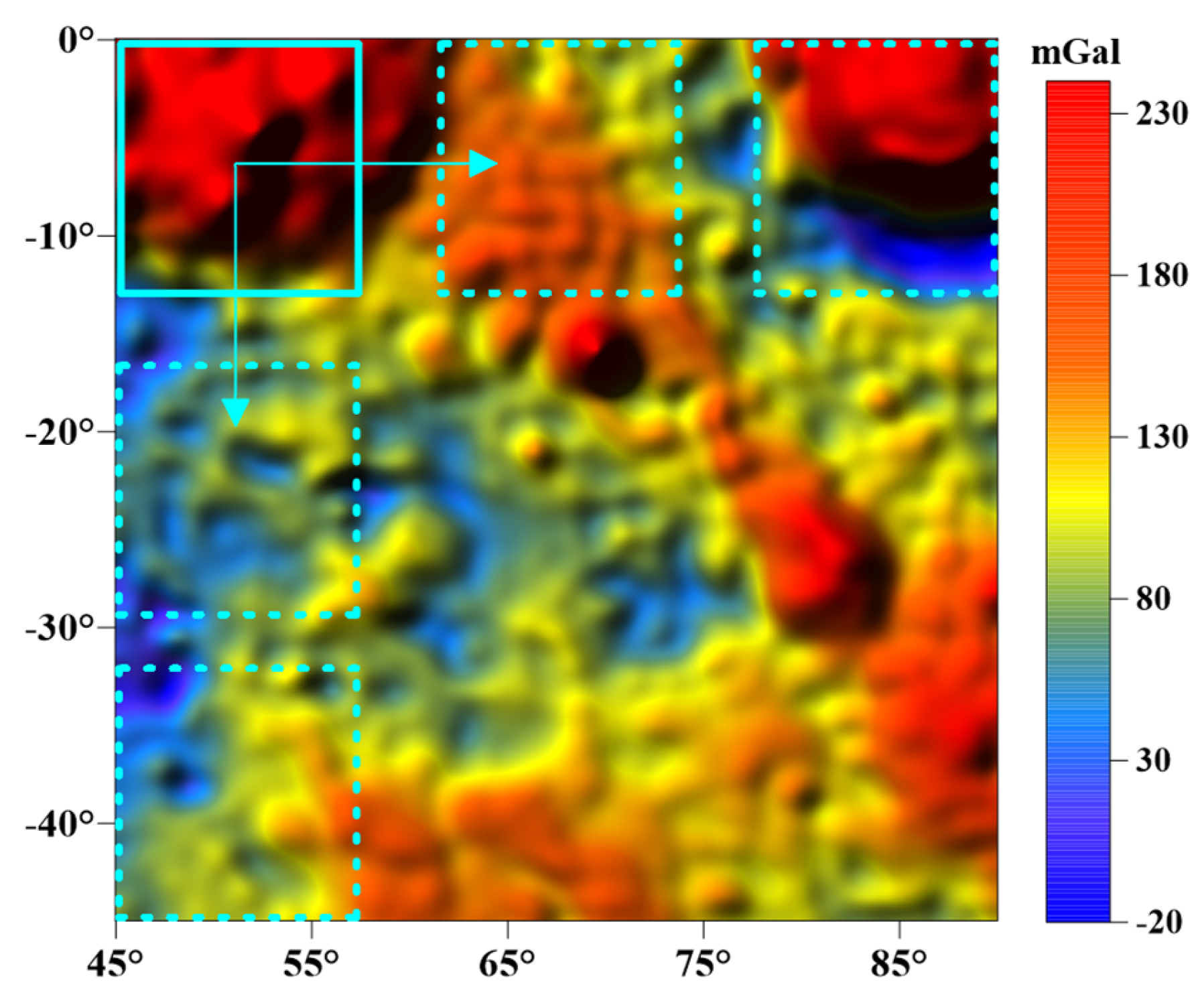
Specifically, in this study, the original lunar Bouguer gravity anomaly data in the regions of longitude 45°~90° and latitude −45°~0° were selected and the grid spacing was 0.075°, with the data filtered in all directions [5] to obtain smooth denoising results (as shown in Figure 3). The moving window was used to cut the denoising mesh, the window size was selected as the sample size (160 × 160), the moving step was 4 times the grid spacing, and 12,100 pieces of sample label data were obtained. For each piece of sample label data, we added the noise data generated through simulation in the following way:

$$\mathbf{R}(x,y)={\displaystyle {\sum }_{\alpha }^{{150}^0}\mathrm{A}}\cdot \sin ({\displaystyle \frac{2\pi }{\kappa +a}}\cdot (x+\tan \alpha \cdot y))+R_0$$

(7)

where $\mathrm{A}$ is the simulated stripe noise amplitude, $\kappa$ is the wavelength, $\alpha$ is the direction angle, $a$ is the wavelength difference, and ${\mathrm{R}}_0$ is white Gaussian noise.

In this study, $\mathrm{A}=1$, $\kappa$ was randomly selected from integers ranging from 3 to 6, $a$ was randomly selected from integers ranging from 1 to 8, $\alpha =0^0, {30}^0, {60}^0, {90}^0, {120}^0, {150}^0$, R represents stripe noise in 6 directions, and ${\mathrm{R}}_0$ is white Gaussian noise with a standard deviation of 1 and a mean of 0.

In this paper, we introduce a noise model, as illustrated in Equation (7), which builds upon and partially modifies the ODF method. In this equation, $\alpha$ governs the direction of the band noise, $\kappa$ controls the wavelength of the band noise, and $a$ regulates the wavelength difference between distinct band noises. The initial determination of these parameter values is rooted in a comprehensive analysis of the characteristics observed in the measured lunar gravity anomaly band noise.

However, to accurately simulate the noise characteristics present in lunar satellite gravity anomalies, we adopted a more rigorous approach. Specifically, we utilized the loss curve obtained from deep learning training and the denoising efficacy on actual data as our evaluation metrics. Through an extensive series of comparative experiments involving the selection of numerous parameter values, we meticulously screened and ultimately identified the optimal parameter settings outlined above.

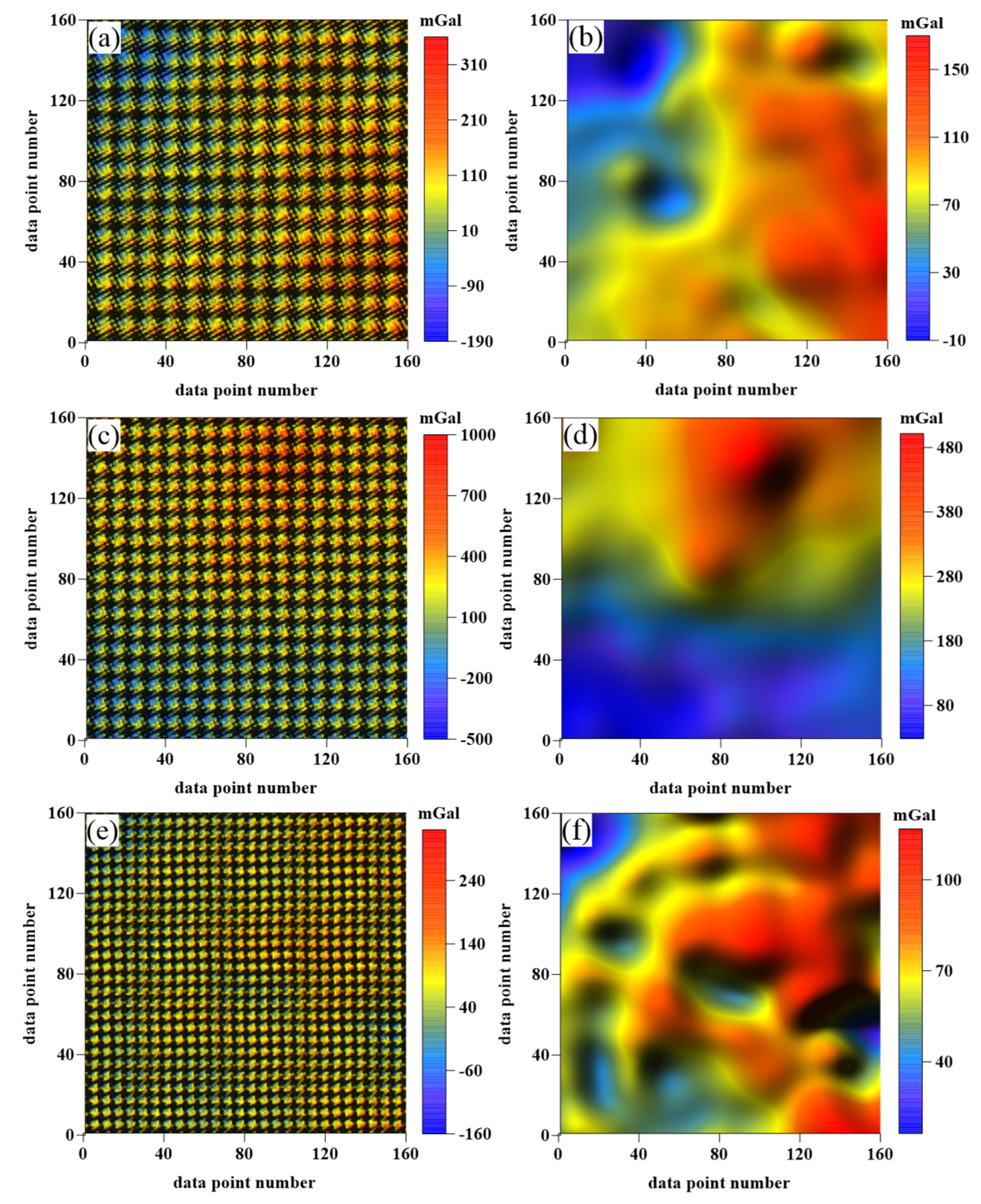
By summing the sample label data with the noise data generated through simulation, 12,100 samples and corresponding labels were obtained. The first 10,100 samples were selected as the training set and the last 2000 samples were selected as the verification set. Figure 4 shows the samples and labels with serial numbers 11, 200, and 2100, respectively. The sample data with noise are shown on the left, and the label data without noise are shown on the right.

3. Results

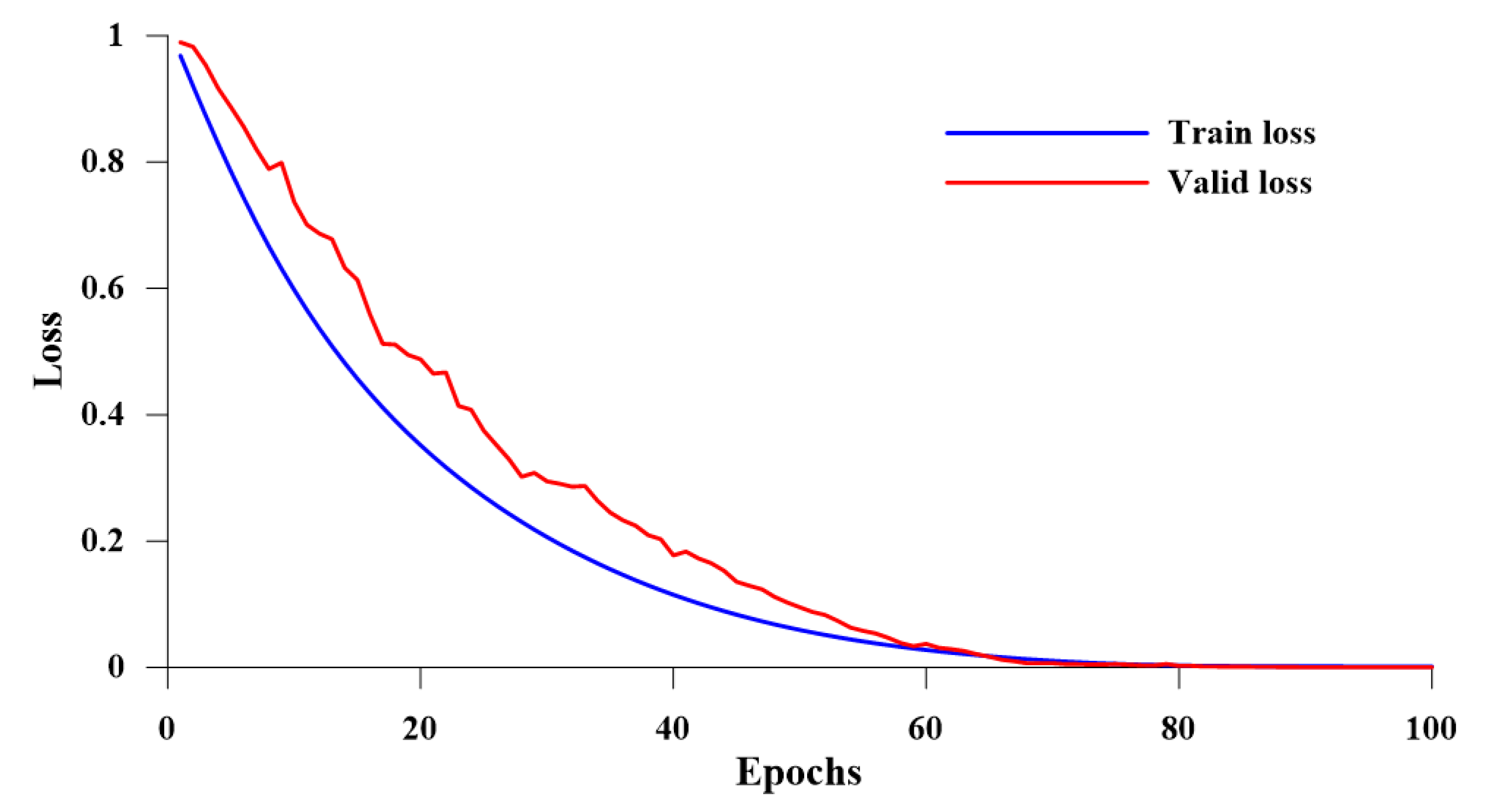
After completing the construction of the deep neural network architecture and preparing the training and validation data sets, the neural network training process can commence. The fundamental stages in the process of model training encompass the following: firstly, the data are fed into the model in manageable batches, with forward propagation employed to ascertain the predicted values. Secondly, backward propagation is implemented to update the model’s weights based on the discrepancy between the predicted and actual values. Lastly, the validation data set is harnessed to assess the model’s performance, with hyperparameters being adjusted to mitigate the risks of both overfitting and underfitting. Through the above steps, with testing and frequent adjustment of the key hyperparameters, the learning rate was recorded as 0.01, the batch size was 60, the dropout was 0.2, and the loss function threshold was 0.0001. In this study, the Adam algorithm was used to optimize deep neural network parameters. The computer was configured as AMD Ryzen 97945HX with Radeon Graphics 2.50 GHz, RAM 16.0 GB, PyTorch version 2.1.2. The loss curves of the training set and verification set are shown in Figure 5. In the initial stage of training, the losses of both the training set and verification set are large; with the increase in the number of iterations, however, the loss curves decay rapidly, and lastly, the two loss curves tend to be stable and close to zero, without overfitting or underfitting. The application effects of the proposed method in synthetic and real data are described below.

3.1. Synthetic Data Test

Figure 6 shows the synthetic data, constructed in the same way as in the previous section, where Figure 6a is the model data with noise, Figure 6b is the model data without noise, and Figure 6c is the noise contained in the model data (the difference between a and b). It can be seen that the lunar Bouguer gravity anomaly generally presents a distribution pattern of high in the middle and low in the periphery; however, it is almost submerged by the stripe noise of multi-directional fusion.

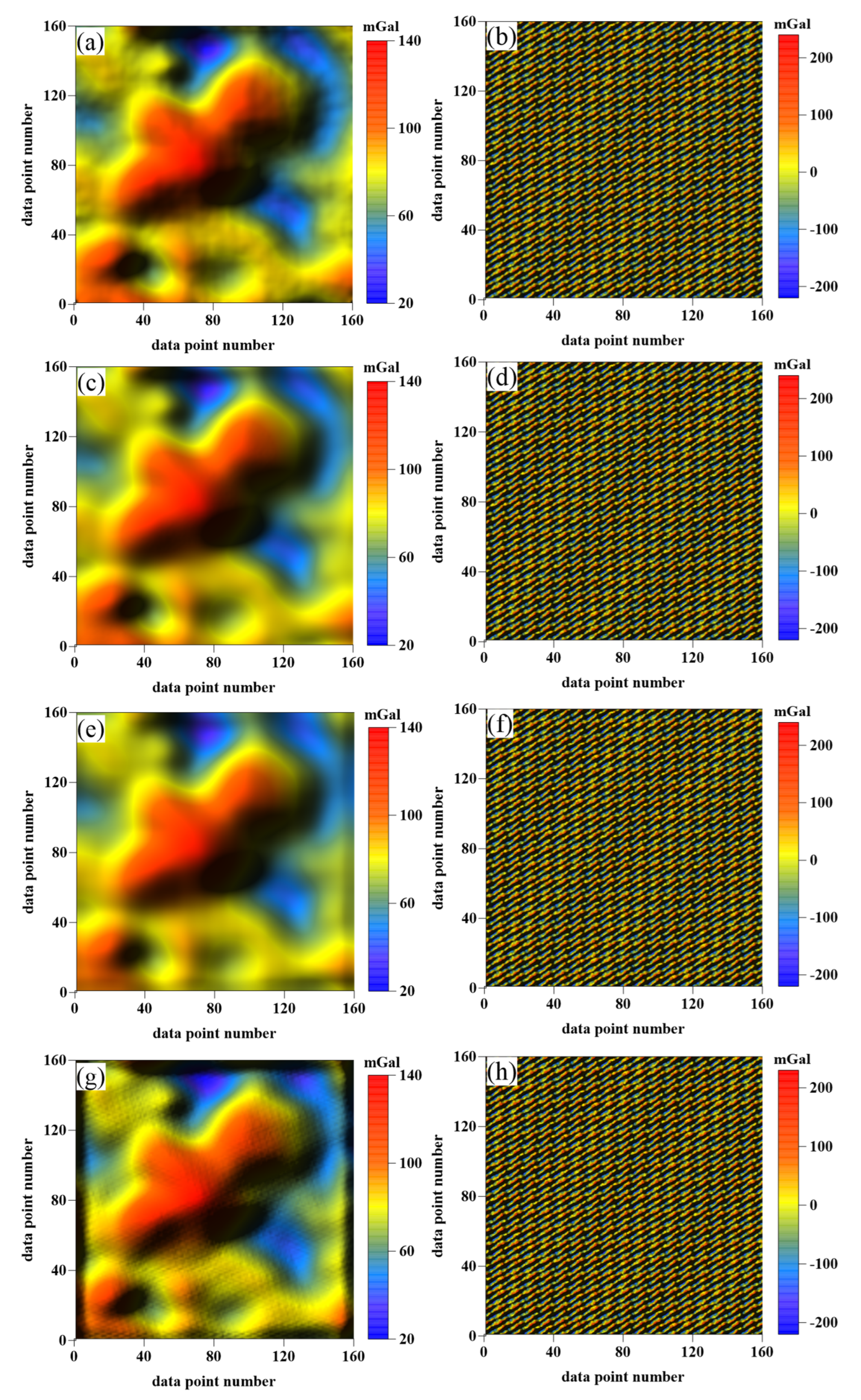
The denoising outcomes achieved using various methods are presented in Figure 7. The denoising result shown in Figure 7a can be obtained by learning the U-Net neural network built in this study, and Figure 7b shows the noise removed by the U-Net neural network. Compared with Figure 6b,c, most of the noise has been removed; however, a small proportion of high-frequency interference is still present. To further enhance the denoising performance of the U-Net neural network, we applied the GF method to smooth the network’s output. The results of this optimization process are presented in Figure 7c, with Figure 7d showing the noise that has been removed. The results for the GF method alone are shown in Figure 7e, and Figure 7f shows the noise removed using the GF method (Gaussian kernel size: 9, standard deviation: 1.6, and iteration number: 3), where it can be seen that there are problems of effective signal loss and boundary effects in the results. The denoising results of the ODF method (filtering window: 11; iteration number: 5) are illustrated in Figure 7g,h, which are still unsatisfactory in many locations, particularly at the edges due to the large noise amplitude of the synthetic data and the wavelengths of the noise, with some effective signals being similar.

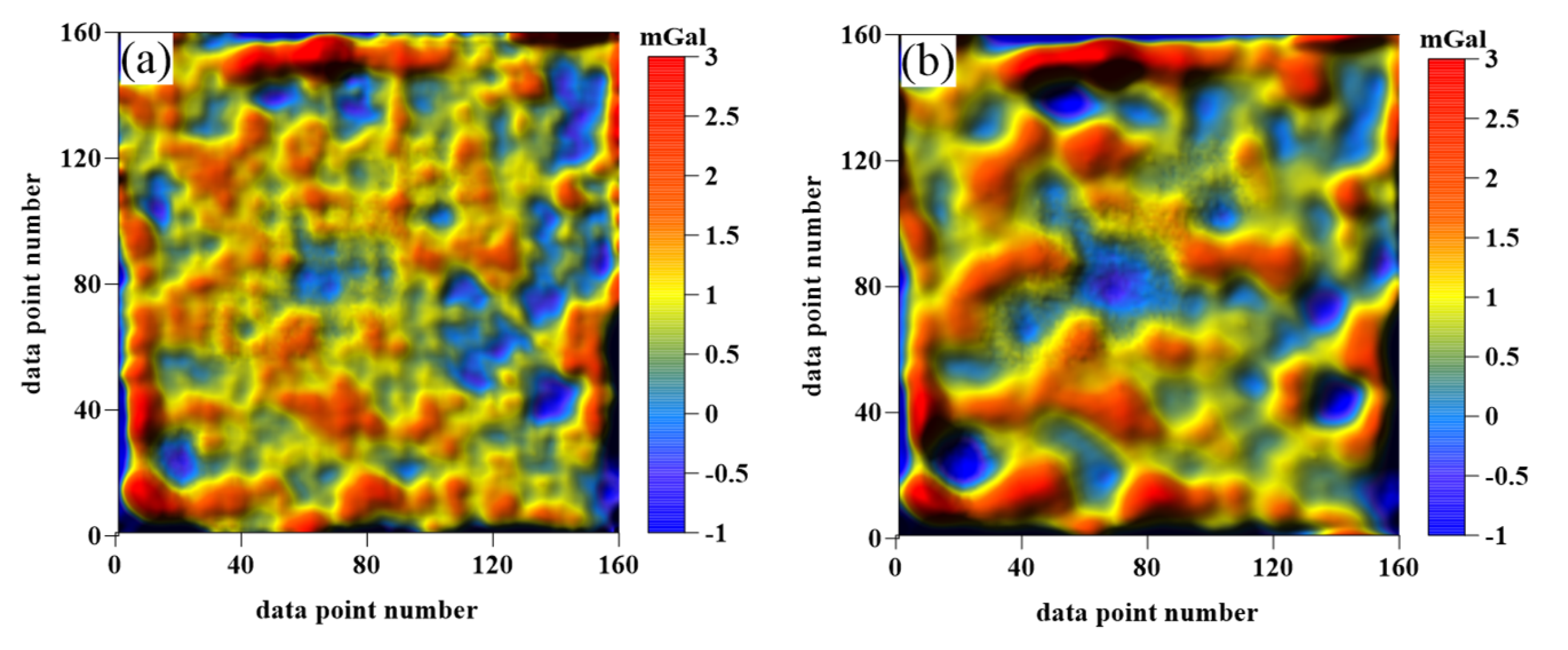
Figure 8 reflects the difference between the true values before and after optimization. In particular, Figure 8a shows the difference between the U-Net denoising result (Figure 7a) and the true value (Figure 6b), and Figure 8b shows the difference between the U-Net + GF denoising result (Figure 7c) and the true value (Figure 6b). It can be seen that not only is the residual noise removed but also that a smoother denoising result is obtained.

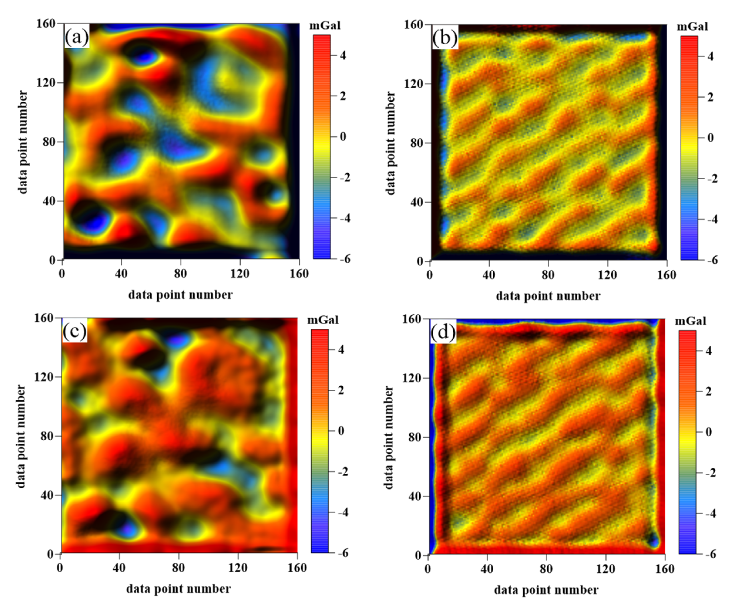
To demonstrate the superiority of the method proposed in this paper, we calculated the difference between the denoising results of the other two filtering methods and the true values, as shown in Figure 9a,b. In addition, we also calculated the standard deviations of the differences between the different methods (GF method, ODF method, and the method proposed in this paper) and the true values, which were 2.99 mGal, 3.27 mGal, and 0.98 mGal, respectively. In addition, to further clarify the differences between different methods, we also provide difference graphs showing the differences between the results of various filtering methods, as shown in Figure 9c,d.

In summary, the denoising method proposed in this paper obtained satisfactory denoising results, which are evidently superior to those of the ODF method and the traditional GF method on synthetic data.

3.2. Real Data Test

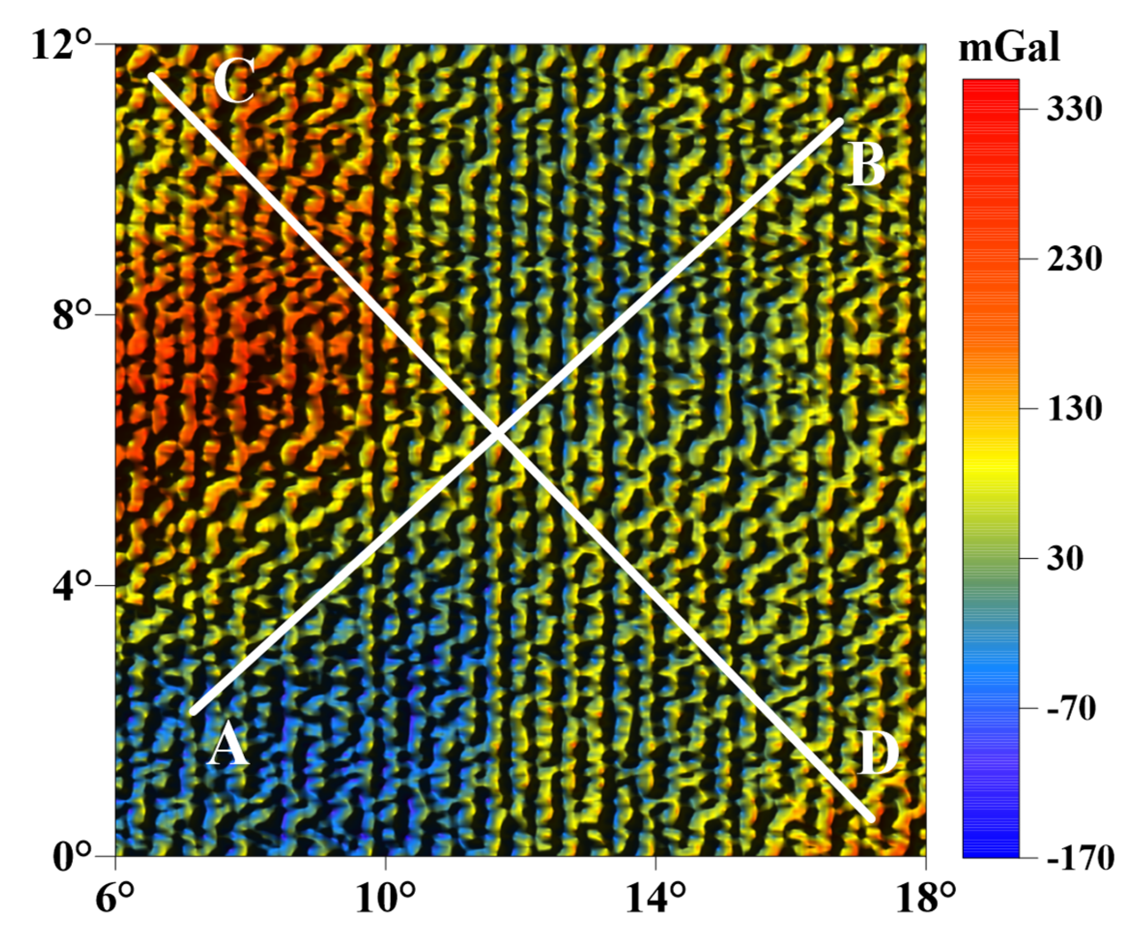
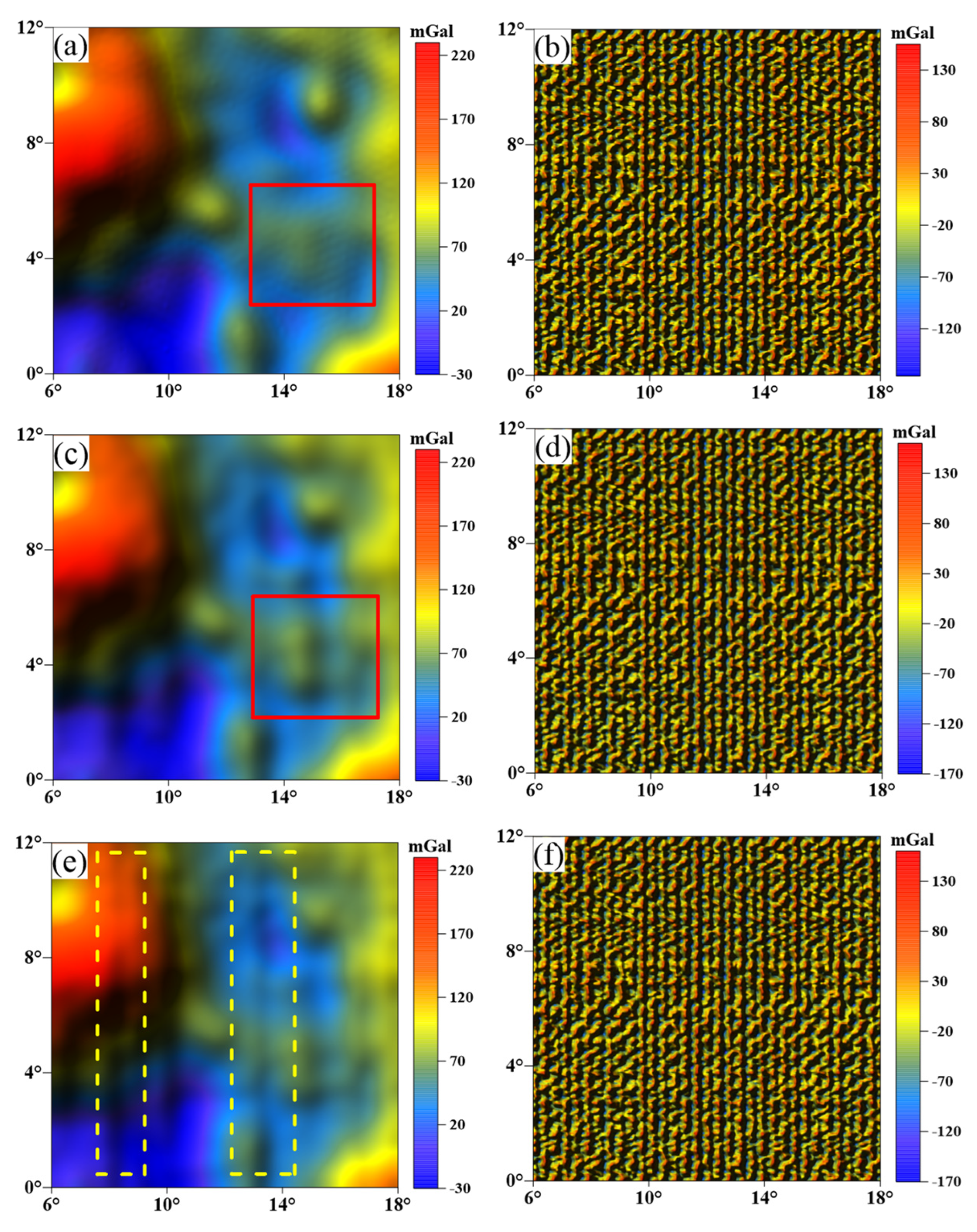
Based on satisfactory denoising results obtained from the synthetic data, the original lunar Bouguer gravity anomaly data (Figure 10) in the region of 6°~18° longitude and 0°~12° latitude were selected for testing, with the grid spacing of 0.075°. The denoising results of the proposed method, ODF method, and GF method were compared, as shown in Figure 10, where Figure 11a is the denoising result of the ODF method, Figure 11b is the noise removed using the ODF method, Figure 11c is the denoising result of the proposed method, Figure 11d is the noise removed using the proposed method, Figure 11e is the denoising result of the GF method, and Figure 11f is the noise removed using the GF method. 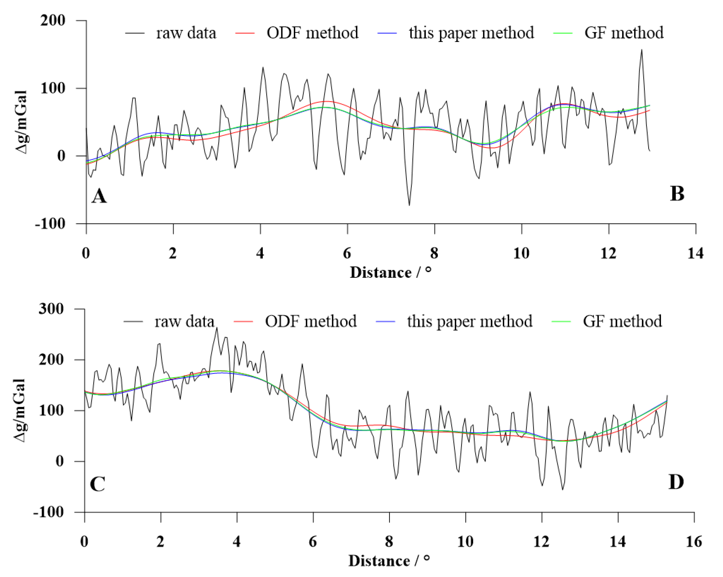Figure 12 shows the curve comparison of the three methods on profile AB and CD.

The profile curves show that all three methods demonstrated commendable denoising capabilities. However, it is important to acknowledge that the amplitude fluctuation of the profile curve approximates 300 mGal, potentially resulting in the suppression of finer anomalies in the data displayed. To better illustrate our results, we developed a planar shadow diagram, as depicted in Figure 11. This diagram showcases the two primary advantages of our novel method. Firstly, our method exhibits superior performance in eliminating band noise, outperforming the GF method, which still leaves residual band noise visible, as indicated by the yellow dashed box in Figure 11e. Secondly, in contrast with the ODF method, our approach preserves some local abnormal information more effectively, as evidenced by the red boxes highlighted in Figure 11a,c.

4. Discussion

4.1. Data Set Construction Method

The data set construction approach outlined in this paper diverges from past research endeavors. Rather than relying on synthetic model forward modeling to procure labeled data, it innovatively employs the filtering outcomes of the ODF method as the labels. Initially, during the exploratory phase of our methodology, we utilized forward modeling for label creation. While this method yielded promising results on both the training and validation data sets, its filtering efficacy on actual data fell short. In response to this limitation, we proposed adopting manually processed results as the labels, upon which we superimpose simulated stripe noise to generate samples that correspond to these labels. This strategic shift not only allows the neural network to learn from human expertise but also enhances its capacity to generalize when confronted with novel data. Ultimately, the practical viability and reliability of our proposed approach were rigorously validated through a combination of synthetic and real data testing.

4.2. Generalization Ability of the Deep Learning Model

The generalization capacity of a deep learning model, which refers to its ability to perform well on unseen data, is a crucial aspect in assessing its effectiveness and robustness. Initially, the model we developed during the early stage of this study exhibited poor generalization, failing to produce satisfactory results on new data sets. Consequently, throughout our research, we consistently enhanced the model’s generalization capacity in several ways. Firstly, we augmented the noise features and quantity within the training set by increasing its number, diversifying stripe noise patterns, and adjusting the signal-to-noise ratio of white noise. Secondly, we expanded the deep learning network from an initial five-layer to a six-layer configuration, enabling the network to more effectively fit complex non-linear data. Lastly, we tuned various hyperparameters, such as the learning rate, batch size, loss function, and loss threshold. By learning from our countless experimental failures and continuously optimizing these parameters, we ultimately attained satisfactory outcomes in both synthetic and real data, thereby confirming the strong generalization capacity of the model presented in this study. In the future, we intend to further enhance the model’s generalization capabilities through the two strategies of data augmentation and transfer learning.

4.3. Selection of Hyperparameters

In this study, we determined the hyperparameters using different trial and error methods. The hyperparameters of deep learning primarily encompass the learning rate, batch size, loss function, and loss threshold, among others. To ascertain the optimal combination of these parameters, we embarked on an extensive testing phase, which necessitated substantial time and computational resources. Specifically, we experimented with learning rates of 0.1, 0.01, 0.001, and 0.0001; batch sizes of 30, 60, 80, and 120; loss functions including Dice and MSE; and loss thresholds of 0.001, 0.005, 0.0001, and 0.0005. After meticulously analyzing the results, we determined that the optimal settings were a learning rate of 0.01, a batch size of 60, the Dice loss function, and a loss threshold of 0.0001. In future studies, we will attempt to use automated methods to optimize the hyperparameters.

5. Conclusions

In this paper, we introduce a methodology for eliminating intricate stripe noise and random noise from lunar gravity anomaly data, utilizing prior knowledge-based deep learning techniques. The construction method of a deep learning network and data set, in addition to the optimization method of deep learning results, is introduced in detail, and synthetic and real data are tested. The results show that the proposed method can effectively remove the stripe noise and random noise in the original lunar Bouguer gravity anomaly data and retain the gravity anomalies caused by the lunar geological structure.

During data set construction, a large amount of label data are generated by the manual processing results of moving window clipping, and the training input data are obtained through the superposition and fusion of stripe noise in six directions on the basis of the label. The advantage of this process is that the deep learning network can not only fully absorb the knowledge of manual denoising but also learn comprehensive and complex stripe noise information. In this way, the denoising results of other areas outside the training area are predicted to be close to or even better than that of manual processing.

In addition, compared with the ODF method and GF method, the proposed method does not require the filter window size to be adjusted through manual trial and error and can quickly and automatically remove the stripe and retain the effective signal through the trained network. The method proposed in this paper can be extended to remove complex banding noise from the gravity anomaly data of other planets or other geophysical data.