


Co-Response of Atmospheric NO2 and CO2 Concentrations from Satellites Observations of Anthropogenic CO2 Emissions for Assessing the Synergistic Effects of Pollution and Carbon Reduction


Abstract
1. Introduction
2. Materials and Methods
2.1. Study Area and Data
2.2. Data Reprocessing and Analysis
- (1)
- Data integration processing
- (2)
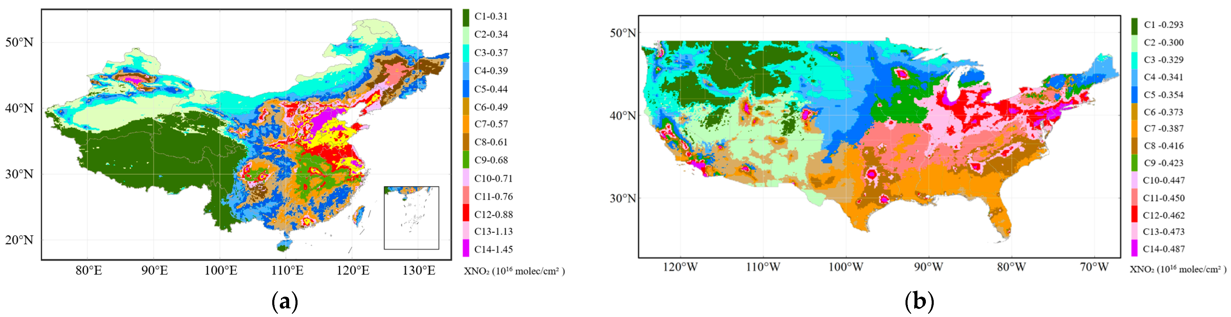
- Clustering of NO2 concentration spatiotemporal features in the study area
- (3)
- Analysis of the response of NO2 and CO2 concentrations to anthropogenic CO2 emissions to assess the synergistic effects of pollution and carbon reduction
3. Results
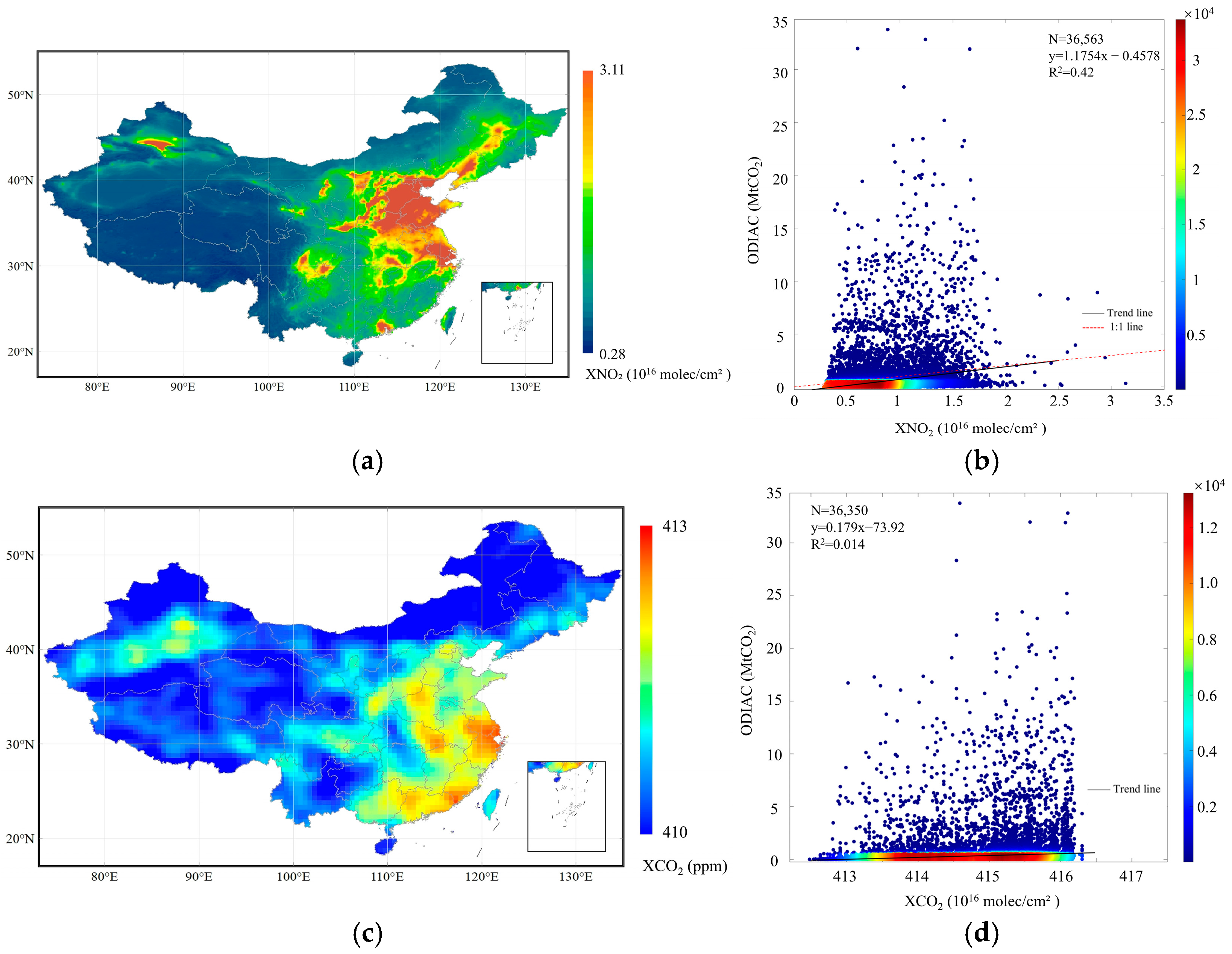
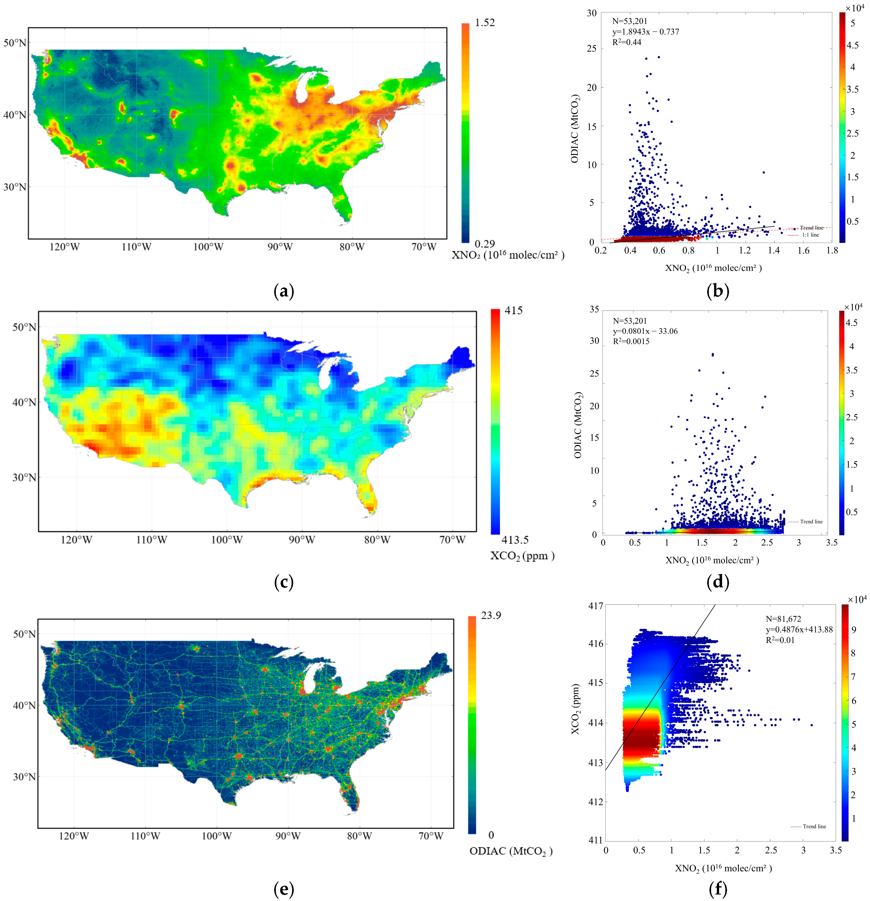
3.1. Spatial and Timely Responding Patterns of NO2 and CO2 Concentrations to Anthropogenic CO2 Emissions
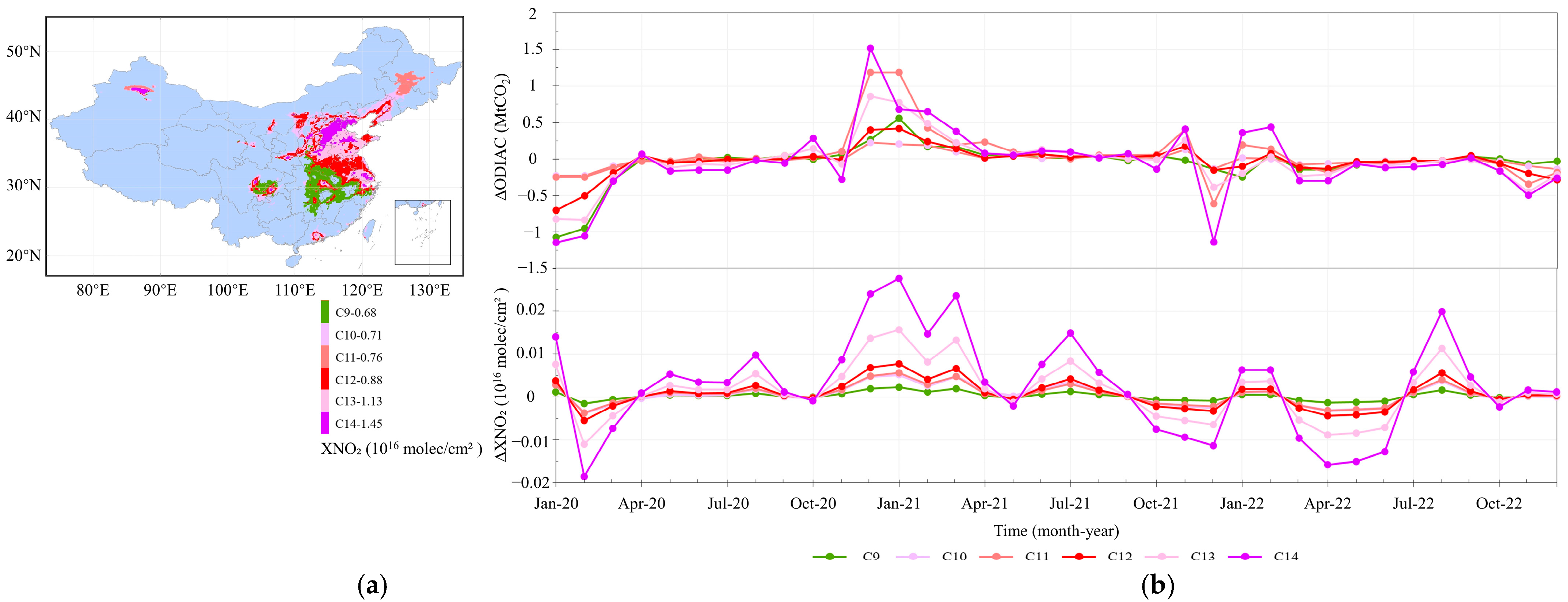
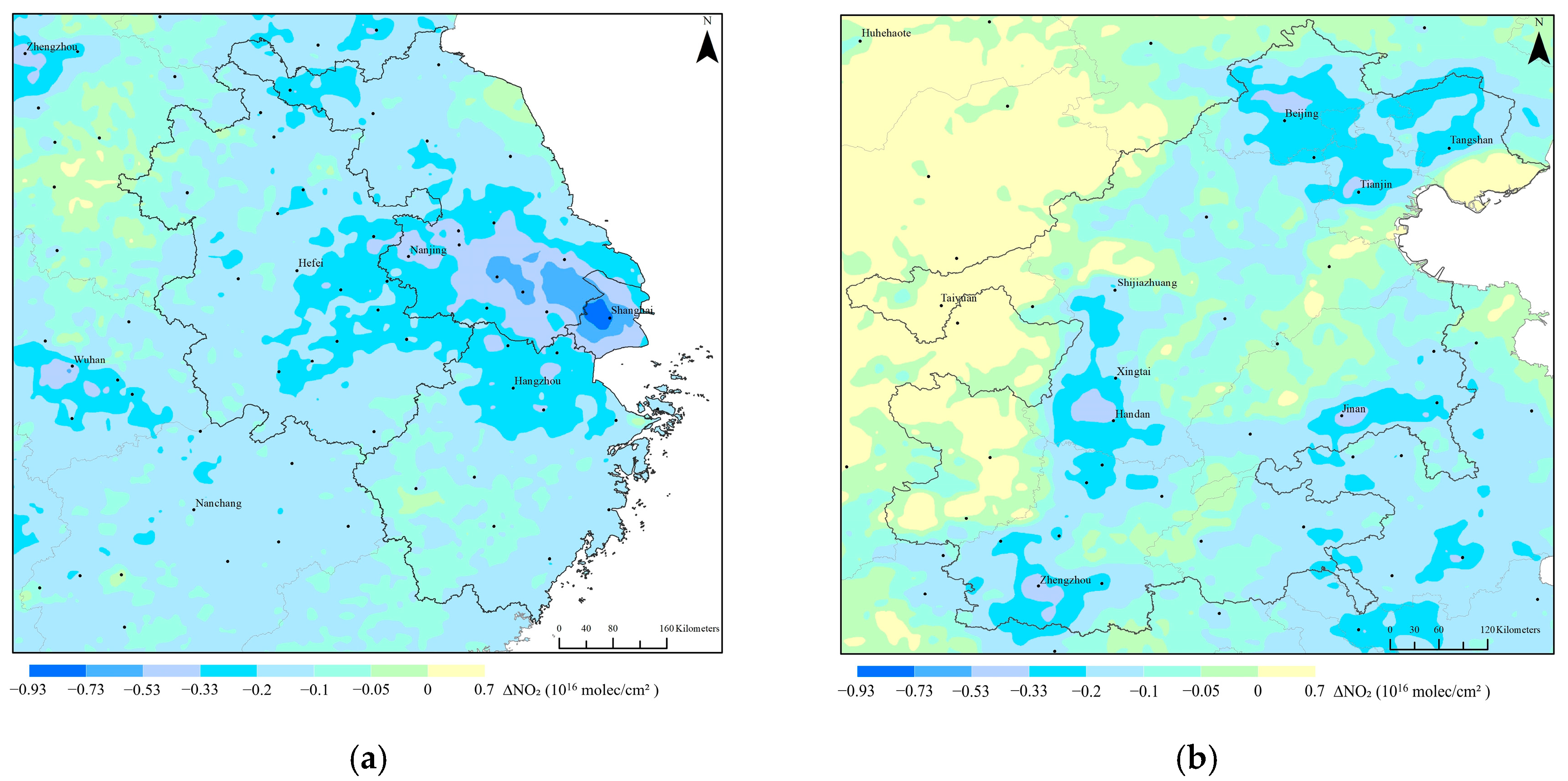
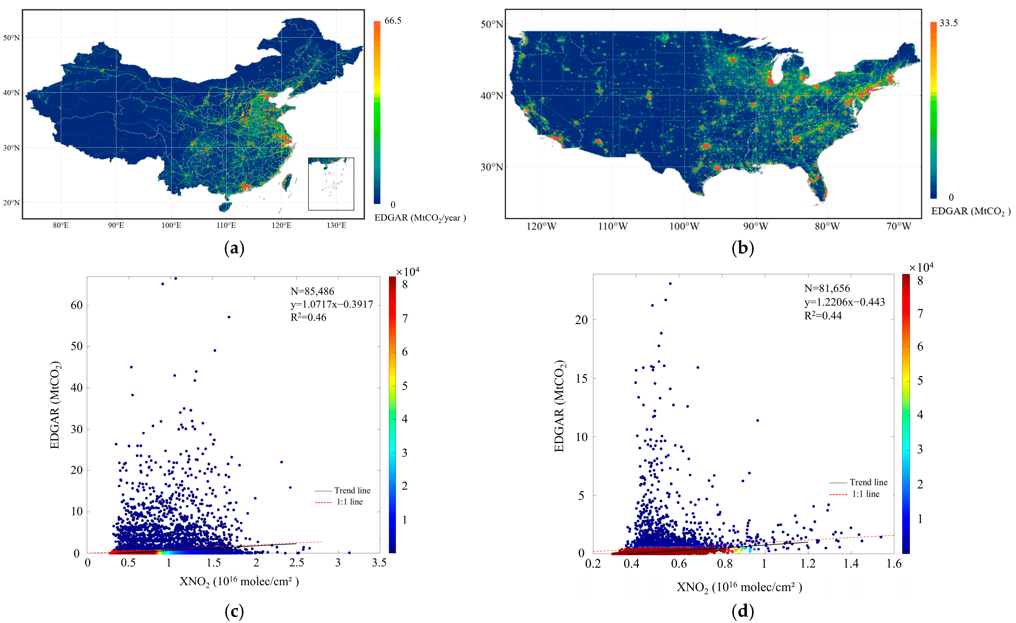
3.1.1. Responding Pattern of Spatial Variations
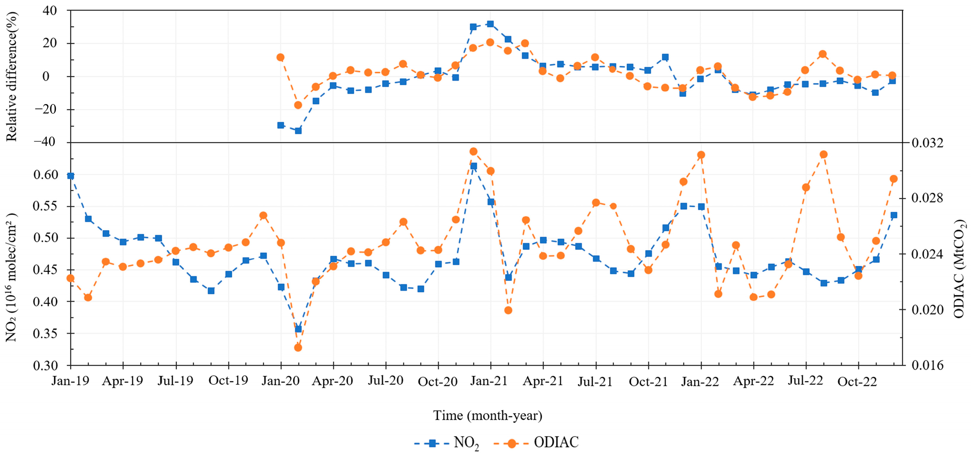
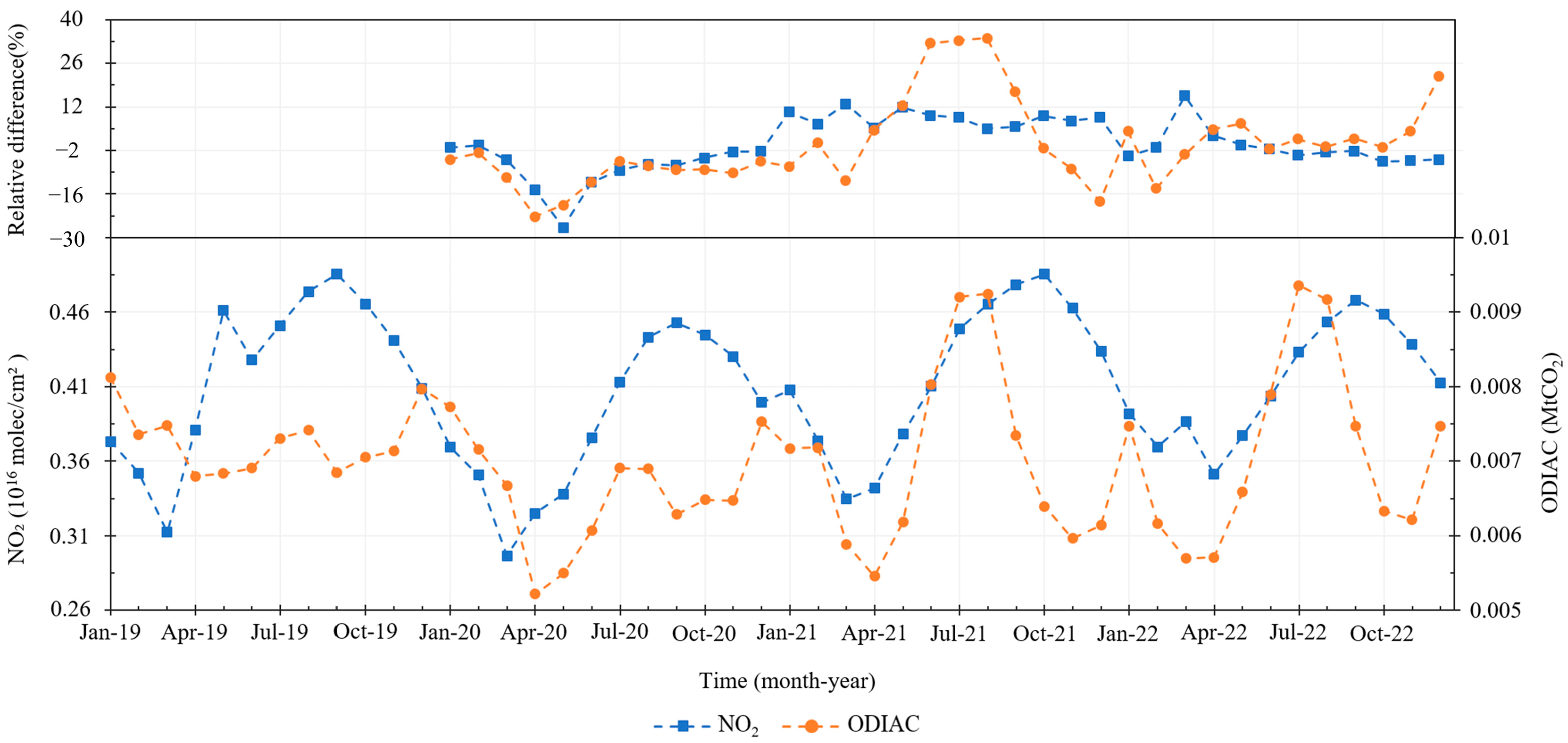
3.1.2. Time Variability with Human Emission Activity
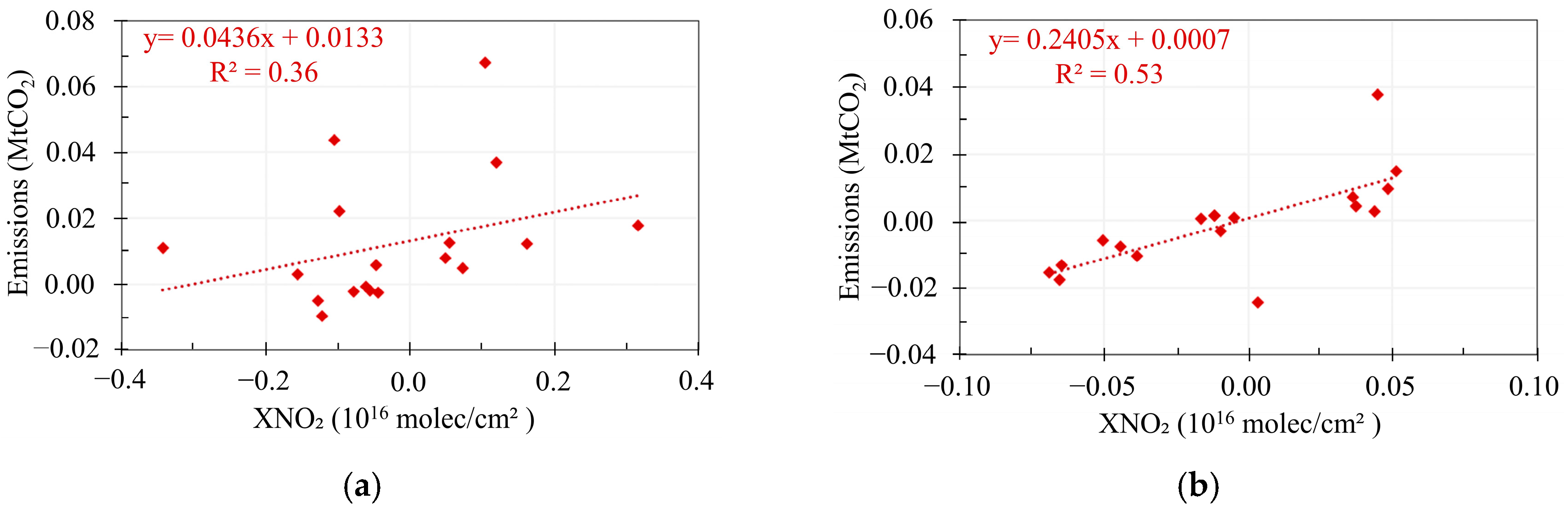
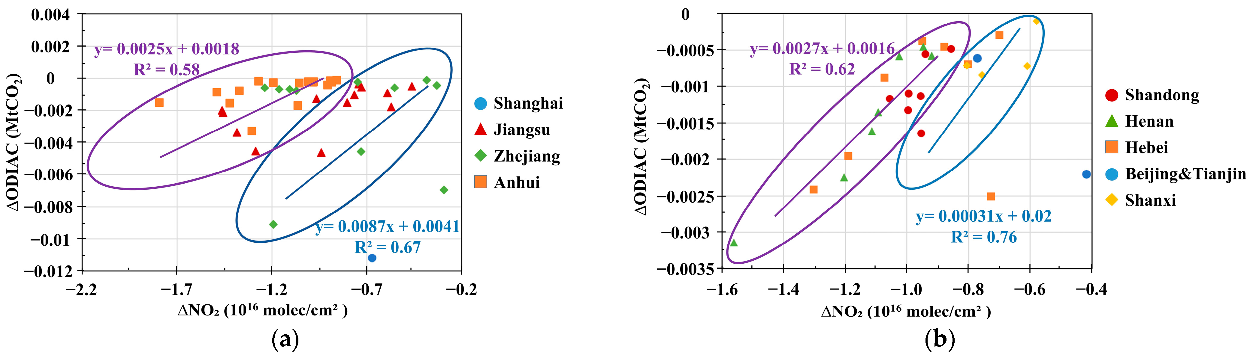
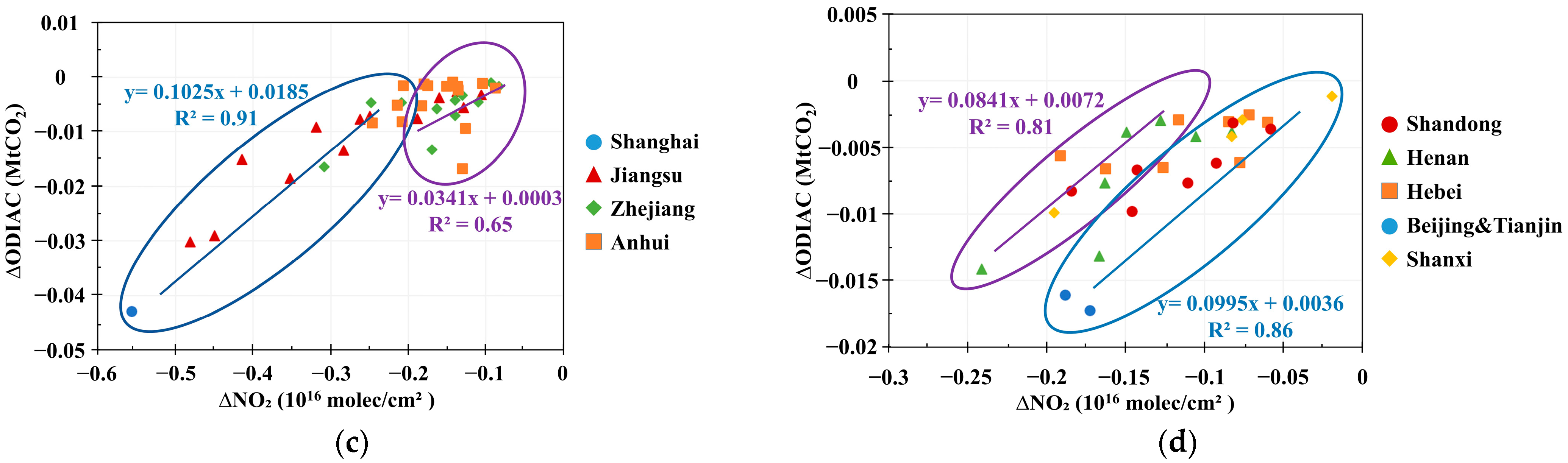
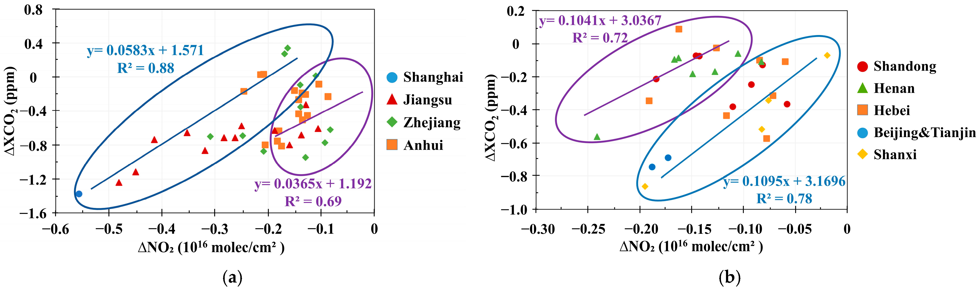
3.2. Co-Response of NO2 and CO2 Concentrations to Anthropogenic CO2 Emissions in the Special Scenarios of Human Activity
4. Discussion
5. Conclusions
Author Contributions
Funding
Data Availability Statement
Acknowledgments
Conflicts of Interest
Appendix A


| Emission Subsector | Beijing | Tianjin | Hebei | Anhui | Jiangsu |
|---|---|---|---|---|---|
| Total Emissions | 159.76 | 311.09 | 1771.01 | 770.70 | 1635.36 |
| Petroleum Processing and Coking | 1.42/0.89 | 9.17/2.95 | 10.5/0.59 | 110.07/14.28 | 6.57/0.40 |
| Raw Chemical Materials and Chemical Products | 0.21/0.13 | 2.61/0.84 | 20.17/1.14 | 70.54/9.15 | 26.39/1.61 |
| Nonmetal Mineral Products | 2.42/1.52 | 7.14/2.30 | 85.32/4.82 | 20.69/2.68 | 104.20/6.37 |
| Smelting and Pressing of Ferrous Metals | 0.04/0.03 | 3.12/1.00 | 752.66/42.50 | 220.11/28.56 | 368.50/22.53 |
| Smelting and Pressing of Nonferrous Metals | 0.01/0.01 | 0.80/0.26 | 1.20/0.07 | 1.76/0.23 | 3.56/0.22 |
| Metal Products | 0.50/0.31 | 1.47/0.47 | 2.05/0.12 | 2.42/0.31 | 2.54/0.16 |
| Production and Supply of Electric Power, Steam, and Hot Water | 62.42/39.07 | 139.86/44.96 | 684.19/38.63 | 283.88/36.83 | 921.72/56.36 |
| Production and Supply of Gas | 0.24/0.15 | 0.12/0.04 | 0.10/0.01 | 1.710.22 | 3.49/0.21 |
| Construction | 1.47/0.92 | 7.34/2.36 | 0.55/0.03 | 7.77/1.01 | 0.97/0.06 |
| Transportation, Storage, Post and Telecommunication Services | 37.95/23.76 | 17.58/5.65 | 28.32/1.60 | 40.75/5.29 | 191.73/11.72 |
| Emission Subsector | Zhejiang | Shanghai | Shandong | Shanxi | Henan |
| Total Emissions | 884.41 | 388.14 | 1894.33 | 1227.46 | 967.48 |
| Petroleum Processing and Coking | 240.35/27.18 | 11.30/2.91 | 56.33/2.97 | 83.33/6.79 | 5.47/0.57 |
| Raw Chemical Materials and Chemical Products | 80.90/9.15 | 5.38/1.39 | 24.46/1.29 | 6.66/0.54 | 5.79/0.60 |
| Nonmetal Mineral Products | 102.47/11.59 | 4.94/1.27 | 140.27/7.40 | 51.76/4.22 | 91.07/9.41 |
| Smelting and Pressing of Ferrous Metals | 32.23/3.64 | 43.68/11.25 | 207.63/10.96 | 305.82/24.91 | 198.72/20.54 |
| Smelting and Pressing of Nonferrous Metals | 2.25/0.25 | 7.62/1.96 | 76.73/4.05 | 27.84/2.27 | 27.34/2.83 |
| Metal Products | 3.13/0.35 | 0.89/0.23 | 11.80/0.62 | 2.41/0.20 | 2.17/0.22 |
| Production and Supply of Electric Power, Steam, and Hot Water | 259.82/29.38 | 188.94/48.68 | 1158.47/61.15 | 741.92/60.44 | 510.15/52.73 |
| Production and Supply of Gas | 0.22/0.03 | 4.79/1.23 | 0.97/0.05 | 0.36/0.03 | 1.23/0.13 |
| Construction | 8.92/1.01 | 4.15/1.07 | 5.26/0.28 | 3.50/0.29 | 16.02/1.66 |
| Transportation, Storage, Post and Telecommunication Services | 59.39/6.72 | 90.56/23.33 | 171.57/9.06 | 29.75/2.42 | 69.16/7.15 |
References
- Wang, H.; Liu, Z.; Zhang, Y.; Yu, Z.; Chen, C. Impact of Different Urban Canopy Models on Air Quality Simulation in Chengdu, Southwestern China. Atmos. Environ. 2021, 267, 118775. [Google Scholar] [CrossRef]
- Liang, M.; Zhang, Y.; Ma, Q.; Yu, D.; Chen, X.; Cohen, J.B. Dramatic Decline of Observed Atmospheric CO2 and CH4 during the COVID-19 Lockdown over the Yangtze River Delta of China. J. Environ. Sci. 2023, 124, 712–722. [Google Scholar] [CrossRef] [PubMed]
- Fang, S.; Du, R.; Qi, B.; Ma, Q.; Zhang, G.; Chen, B.; Li, J. Variation of Carbon Dioxide Mole Fraction at a Typical Urban Area in the Yangtze River Delta, China. Atmos. Res. 2022, 265, 105884. [Google Scholar] [CrossRef]
- Liu, L.; Chen, L.; Liu, Y.; Yang, D.; Zhang, X.; Lu, N.; Ju, W.; Jiang, F.; Yin, Z.; Liu, G.; et al. Satellite Remote Sensing for Global Stocktaking: Methods, Progress and Perspectives. Natl. Remote Sens. Bull. 2022, 26, 243–267. [Google Scholar] [CrossRef]
- Canadell, J.G.; Le Quéré, C.; Raupach, M.R.; Field, C.B.; Buitenhuis, E.T.; Ciais, P.; Conway, T.J.; Gillett, N.P.; Houghton, R.A.; Marland, G. Contributions to Accelerating Atmospheric CO2 Growth from Economic Activity, Carbon Intensity, and Efficiency of Natural Sinks. Proc. Natl. Acad. Sci. USA 2007, 104, 18866–18870. [Google Scholar] [CrossRef] [PubMed]
- Ritchie, H.; Roser, M. CO2 Emissions. Our World Data 2020. Available online: https://ourworldindata.org/co2-emissions (accessed on 6 March 2024).
- Hsueh, Y.-H.; Li, K.-F.; Lin, L.-C.; Bhattacharya, S.K.; Laskar, A.H.; Liang, M.-C. East Asian CO2 Level Change Caused by Pacific Decadal Oscillation. Remote Sens. Environ. 2021, 264, 112624. [Google Scholar] [CrossRef]
- Goldberg, D.L.; Lu, Z.; Oda, T.; Lamsal, L.N.; Liu, F.; Griffin, D.; McLinden, C.A.; Krotkov, N.A.; Duncan, B.N.; Streets, D.G. Exploiting OMI NO2 Satellite Observations to Infer Fossil-Fuel CO2 Emissions from U.S. Megacities. Sci. Total Environ. 2019, 695, 133805. [Google Scholar] [CrossRef]
- Konovalov, I.B.; Berezin, E.V.; Ciais, P.; Broquet, G.; Zhuravlev, R.V.; Janssens-Maenhout, G. Estimation of Fossil-Fuel CO2 Emissions Using Satellite Measurements of “Proxy” Species. Atmos. Chem. Phys. 2016, 16, 13509–13540. [Google Scholar] [CrossRef]
- Liu, F.; Duncan, B.N.; Krotkov, N.A.; Lamsal, L.N.; Beirle, S.; Griffin, D.; McLinden, C.A.; Goldberg, D.L.; Lu, Z. A Methodology to Constrain Carbon Dioxide Emissions from Coal-Fired Power Plants Using Satellite Observations of Co-Emitted Nitrogen Dioxide. Atmos. Chem. Phys. 2020, 20, 99–116. [Google Scholar] [CrossRef]
- Shim, C.; Han, J.; Henze, D.K.; Yoon, T. Identifying Local Anthropogenic CO2 Emissions with Satellite Retrievals: A Case Study in South Korea. Int. J. Remote Sens. 2019, 40, 1011–1029. [Google Scholar] [CrossRef]
- Kataoka, F.; Crisp, D.; Taylor, T.; O’Dell, C.; Kuze, A.; Shiomi, K.; Suto, H.; Bruegge, C.; Schwandner, F.; Rosenberg, R.; et al. The Cross-Calibration of Spectral Radiances and Cross-Validation of CO2 Estimates from GOSAT and OCO-2. Remote Sens. 2017, 9, 1158. [Google Scholar] [CrossRef]
- Jin, C.; Xue, Y.; Jiang, X.; Zhao, L.; Yuan, T.; Sun, Y.; Wu, S.; Wang, X. A Long-Term Global XCO2 Dataset: Ensemble of Satellite Products. Atmos. Res. 2022, 279, 106385. [Google Scholar] [CrossRef]
- Kuhlmann, G.; Broquet, G.; Marshall, J.; Clément, V.; Löscher, A.; Meijer, Y.; Brunner, D. Detectability of CO2 Emission Plumes of Cities and Power Plants with the Copernicus Anthropogenic CO2 Monitoring (CO2M) Mission. Atmos. Meas. Tech. 2019, 12, 6695–6719. [Google Scholar] [CrossRef]
- He, Q.; Ye, T.; Wang, W.; Luo, M.; Song, Y.; Zhang, M. Spatiotemporally Continuous Estimates of Daily 1-Km PM2.5 Concentrations and Their Long-Term Exposure in China from 2000 to 2020. J. Environ. Manag. 2023, 342, 118145. [Google Scholar] [CrossRef]
- Park, H.; Jeong, S.; Park, H.; Labzovskii, L.D.; Bowman, K.W. An Assessment of Emission Characteristics of Northern Hemisphere Cities Using Spaceborne Observations of CO2, CO, and NO2. Remote Sens. Environ. 2021, 254, 112246. [Google Scholar] [CrossRef]
- Hakkarainen, J.; Ialongo, I.; Maksyutov, S.; Crisp, D. Analysis of Four Years of Global XCO2 Anomalies as Seen by Orbiting Carbon Observatory-2. Remote Sens. 2019, 11, 850. [Google Scholar] [CrossRef]
- Reuter, M.; Buchwitz, M.; Schneising, O.; Krautwurst, S.; O’Dell, C.W.; Richter, A.; Bovensmann, H.; Burrows, J.P. Towards Monitoring Localized CO2 Emissions from Space: Co-Located Regional CO2 and NO2 Enhancements Observed by the OCO-2 and S5P Satellites. Atmos. Chem. Phys. 2019, 19, 9371–9383. [Google Scholar] [CrossRef]
- Lei, L.; Zhong, H.; He, Z.; Cai, B.; Yang, S.; Wu, C.; Zeng, Z.; Liu, L.; Zhang, B. Assessment of Atmospheric CO2 Concentration Enhancement from Anthropogenic Emissions Based on Satellite Observations. Chin. Sci. Bull. 2017, 62, 2941–2950. [Google Scholar] [CrossRef]
- Buchwitz, M.; Reuter, M.; Noël, S.; Bramstedt, K.; Schneising, O.; Hilker, M.; Fuentes Andrade, B.; Bovensmann, H.; Burrows, J.P.; Di Noia, A.; et al. Can a Regional-Scale Reduction of Atmospheric CO2 during the COVID-19 Pandemic Be Detected from Space? A Case Study for East China Using Satellite XCO2 Retrievals. Atmos. Meas. Tech. 2021, 14, 2141–2166. [Google Scholar] [CrossRef]
- Park, C.; Jeong, S.; Park, H.; Yun, J.; Liu, J. Evaluation of the Potential Use of Satellite-Derived XCO2 in Detecting CO2 Enhancement in Megacities with Limited Ground Observations: A Case Study in Seoul Using Orbiting Carbon Observatory-2. Asia-Pac. J. Atmos. Sci. 2021, 57, 289–299. [Google Scholar] [CrossRef]
- Hakkarainen, J.; Ialongo, I.; Oda, T.; Szeląg, M.E.; O’Dell, C.W.; Eldering, A.; Crisp, D. Building a Bridge: Characterizing Major Anthropogenic Point Sources in the South African Highveld Region Using OCO-3 Carbon Dioxide Snapshot Area Maps and Sentinel-5P/TROPOMI Nitrogen Dioxide Columns. Environ. Res. Lett. 2023, 18, 035003. [Google Scholar] [CrossRef]
- Hakkarainen, J.; Szeląg, M.E.; Ialongo, I.; Retscher, C.; Oda, T.; Crisp, D. Analyzing Nitrogen Oxides to Carbon Dioxide Emission Ratios from Space: A Case Study of Matimba Power Station in South Africa. Atmos. Environ. X 2021, 10, 100110. [Google Scholar] [CrossRef]
- Yang, E.G.; Kort, E.A.; Ott, L.E.; Oda, T.; Lin, J.C. Using Space-Based CO2 and NO2 Observations to Estimate Urban CO2 Emissions. JGR Atmos. 2023, 128, e2022JD037736. [Google Scholar] [CrossRef]
- Wang, Y.-N.; Li, B.-X.; Zhang, Y.-X.; Zhao, Y.; Miao, C.-K.; An, J.-Q. Spatiotemporal Characteristics and Influencing Factors of the Synergistic Effect of Pollution Reduction and Carbon Reduction in China. Huan Jing Ke Xue = Huanjing Kexue 2024, 45, 4993–5002. [Google Scholar] [PubMed]
- Zhang, W.; Zhang, X.; Liu, L.; Zhao, L.; Lu, X. Spatial Variations in NO2 Trend in North China Plain Based on Multi-Source Satellite Remote Sensing. Natl. Remote Sens. Bull. 2018, 22, 335–346. [Google Scholar] [CrossRef]
- Sheng, M.; Lei, L.; Zeng, Z.-C.; Rao, W.; Zhang, S. Detecting the Responses of CO2 Column Abundances to Anthropogenic Emissions from Satellite Observations of GOSAT and OCO-2. Remote Sens. 2021, 13, 3524. [Google Scholar] [CrossRef]
- Kumari, P.; Toshniwal, D. Impact of Lockdown Measures during COVID-19 on Air Quality—A Case Study of India. Int. J. Environ. Health Res. 2022, 32, 503–510. [Google Scholar] [CrossRef]
- Tang, X.; Snowden, S.; McLellan, B.C.; Höök, M. Clean Coal Use in China: Challenges and Policy Implications. Energy Policy 2015, 87, 517–523. [Google Scholar] [CrossRef]
- Zheng, Y.; Xue, T.; Zhang, Q.; Geng, G.; Tong, D.; Li, X.; He, K. Air Quality Improvements and Health Benefits from China’s Clean Air Action since 2013. Environ. Res. Lett. 2017, 12, 114020. [Google Scholar] [CrossRef]
- Liu, Z.; Deng, Z.; He, G.; Wang, H.; Zhang, X.; Lin, J.; Qi, Y.; Liang, X. Challenges and Opportunities for Carbon Neutrality in China. Nat. Rev. Earth Environ. 2021, 3, 141–155. [Google Scholar] [CrossRef]
- Ross, K.; Chmiel, J.F.; Ferkol, T. The Impact of the Clean Air Act. J. Pediatr. 2012, 161, 781–786. [Google Scholar] [CrossRef] [PubMed]
- Yokota, T.; Yoshida, Y.; Eguchi, N.; Ota, Y.; Tanaka, T.; Watanabe, H.; Maksyutov, S. Global Concentrations of CO2 and CH4 Retrieved from GOSAT: First Preliminary Results. SOLA 2009, 5, 160–163. [Google Scholar] [CrossRef]
- Eldering, A.; Wennberg, P.O.; Crisp, D.; Schimel, D.S.; Gunson, M.R.; Chatterjee, A.; Liu, J.; Schwandner, F.M.; Sun, Y.; O’Dell, C.W.; et al. The Orbiting Carbon Observatory-2 Early Science Investigations of Regional Carbon Dioxide Fluxes. Science 2017, 358, eaam5745. [Google Scholar] [CrossRef]
- Eldering, A.; Taylor, T.E.; O’Dell, C.W.; Pavlick, R. The OCO-3 Mission: Measurement Objectives and Expected Performance Based on 1 Year of Simulated Data. Atmos. Meas. Tech. 2019, 12, 2341–2370. [Google Scholar] [CrossRef]
- Oda, T.; Maksyutov, S. A Very High-Resolution (1 Km × 1 Km) Global Fossil Fuel CO2 Emission Inventory Derived Using a Point Source Database and Satellite Observations of Nighttime Lights. Atmos. Chem. Phys. 2011, 11, 543–556. [Google Scholar] [CrossRef]
- European Commission; Joint Research Centre; IEA. GHG Emissions of All World Countries; Publications Office: Luxembourg, 2024. [Google Scholar]
- Van Geffen, J.; Boersma, K.F.; Eskes, H.; Sneep, M.; Ter Linden, M.; Zara, M.; Veefkind, J.P. S5P TROPOMI NO2 Slant Column Retrieval: Method, Stability, Uncertainties and Comparisons with OMI. Atmos. Meas. Tech. 2020, 13, 1315–1335. [Google Scholar] [CrossRef]
- Fioletov, V.; McLinden, C.A.; Griffin, D.; Krotkov, N.; Liu, F.; Eskes, H. Quantifying Urban, Industrial, and Background Changes in NO2 during the COVID-19 Lockdown Period Based on TROPOMI Satellite Observations. Atmos. Chem. Phys. 2022, 22, 4201–4236. [Google Scholar] [CrossRef]
- Veefkind, J.P.; Aben, I.; McMullan, K.; Förster, H.; De Vries, J.; Otter, G.; Claas, J.; Eskes, H.J.; De Haan, J.F.; Kleipool, Q.; et al. TROPOMI on the ESA Sentinel-5 Precursor: A GMES Mission for Global Observations of the Atmospheric Composition for Climate, Air Quality and Ozone Layer Applications. Remote Sens. Environ. 2012, 120, 70–83. [Google Scholar] [CrossRef]
- OCO-2 Science Team/Michael Gunson, Annmarie Eldering ACOS GOSAT/TANSO-FTS Level 2 Full Physics Standard Product V7.3, Greenbelt, MD, USA. Available online: https://disc.gsfc.nasa.gov/datasets/ACOS_L2S_7.3/summary (accessed on 15 January 2024).
- Taylor, T.E.; Eldering, A.; Merrelli, A.; Kiel, M.; Somkuti, P.; Cheng, C.; Rosenberg, R.; Fisher, B.; Crisp, D.; Basilio, R.; et al. OCO-3 Early Mission Operations and Initial (vEarly) XCO2 and SIF Retrievals. Remote Sens. Environ. 2020, 251, 112032. [Google Scholar] [CrossRef]
- Chen, Y.; Cheng, J.; Song, X.; Liu, S.; Sun, Y.; Yu, D.; Fang, S. Global-Scale Evaluation of XCO2 Products from GOSAT, OCO-2 and CarbonTracker Using Direct Comparison and Triple Collocation Method. Remote Sens. 2022, 14, 5635. [Google Scholar] [CrossRef]
- Wang, T.; Shi, J.; Jing, Y.; Zhao, T.; Ji, D.; Xiong, C. Combining XCO2 Measurements Derived from SCIAMACHY and GOSAT for Potentially Generating Global CO2 Maps with High Spatiotemporal Resolution. PLoS ONE 2014, 9, e105050. [Google Scholar] [CrossRef] [PubMed]
- Chen, X.; He, Q.; Ye, T.; Liang, Y.; Li, Y. Decoding Spatiotemporal Dynamics in Atmospheric CO2 in Chinese Cities: Insights from Satellite Remote Sensing and Geographically and Temporally Weighted Regression Analysis. Sci. Total Environ. 2024, 908, 167917. [Google Scholar] [CrossRef] [PubMed]
- Buchwitz, M.; Reuter, M.; Schneising, O.; Noël, S.; Gier, B.; Bovensmann, H.; Burrows, J.P.; Boesch, H.; Anand, J.; Parker, R.J.; et al. Computation and Analysis of Atmospheric Carbon Dioxide Annual Mean Growth Rates from Satellite Observations during 2003–2016. Atmos. Chem. Phys. 2018, 18, 17355–17370. [Google Scholar] [CrossRef]
- Maksyutov, S.; Takagi, H.; Valsala, V.K.; Saito, M.; Oda, T.; Saeki, T.; Belikov, D.A.; Saito, R.; Ito, A.; Yoshida, Y.; et al. Regional CO2 Flux Estimates for 2009–2010 Based on GOSAT and Ground-Based CO2 Observations. Atmos. Chem. Phys. 2013, 13, 9351–9373. [Google Scholar] [CrossRef]
- Takagi, H.; Saeki, T.; Oda, T.; Saito, M.; Valsala, V.; Belikov, D.; Saito, R.; Yoshida, Y.; Morino, I.; Uchino, O.; et al. On the Benefit of GOSAT Observations to the Estimation of Regional CO2 Fluxes. SOLA 2011, 7, 161–164. [Google Scholar] [CrossRef]
- Oda, T.; Lauvaux, T.; Lu, D.; Rao, P.; Miles, N.L.; Richardson, S.J.; Gurney, K.R. On the Impact of Granularity of Space-Based Urban CO2 Emissions in Urban Atmospheric Inversions: A Case Study for Indianapolis, IN. Elem. Sci. Anthr. 2017, 5, 28. [Google Scholar] [CrossRef]
- Janardanan, R.; Maksyutov, S.; Oda, T.; Saito, M.; Kaiser, J.W.; Ganshin, A.; Stohl, A.; Matsunaga, T.; Yoshida, Y.; Yokota, T. Comparing GOSAT Observations of Localized CO2 Enhancements by Large Emitters with Inventory-based Estimates. Geophys. Res. Lett. 2016, 43, 3486–3493. [Google Scholar] [CrossRef]
- Lauvaux, T.; Miles, N.L.; Deng, A.; Richardson, S.J.; Cambaliza, M.O.; Davis, K.J.; Gaudet, B.; Gurney, K.R.; Huang, J.; O’Keefe, D.; et al. High-resolution Atmospheric Inversion of Urban CO2 Emissions during the Dormant Season of the Indianapolis Flux Experiment (INFLUX). JGR Atmos. 2016, 121, 5213–5236. [Google Scholar] [CrossRef]
- Han, P.; Zeng, N.; Oda, T.; Lin, X.; Crippa, M.; Guan, D.; Janssens-Maenhout, G.; Ma, X.; Liu, Z.; Shan, Y.; et al. Evaluating China’s Fossil-Fuel CO2 Emissions from a Comprehensive Dataset of Nine Inventories. Atmos. Chem. Phys. 2020, 20, 11371–11385. [Google Scholar] [CrossRef]
- Crippa, M.; Guizzardi, D.; Pisoni, E.; Solazzo, E.; Guion, A.; Muntean, M.; Florczyk, A.; Schiavina, M.; Melchiorri, M.; Hutfilter, A.F. Global Anthropogenic Emissions in Urban Areas: Patterns, Trends, and Challenges. Environ. Res. Lett. 2021, 16, 074033. [Google Scholar] [CrossRef]
- Zhang, Q.; Jiang, X.; Tong, D.; Davis, S.J.; Zhao, H.; Geng, G.; Feng, T.; Zheng, B.; Lu, Z.; Streets, D.G.; et al. Transboundary Health Impacts of Transported Global Air Pollution and International Trade. Nature 2017, 543, 705–709. [Google Scholar] [CrossRef] [PubMed]
- McDonald, B.C.; De Gouw, J.A.; Gilman, J.B.; Jathar, S.H.; Akherati, A.; Cappa, C.D.; Jimenez, J.L.; Lee-Taylor, J.; Hayes, P.L.; McKeen, S.A.; et al. Volatile Chemical Products Emerging as Largest Petrochemical Source of Urban Organic Emissions. Science 2018, 359, 760–764. [Google Scholar] [CrossRef] [PubMed]
- Olsson, P.Q.; Benner, R.L. Atmospheric Chemistry and Physics: From Air Pollution to Climate Change by John H. Seinfeld (California Institute of Technology) and Spyros N. Pandis (Carnegie Mellon University). Wiley-VCH: New York. 1997. $89.95. Xxvii + 1326 pp. ISBN 0-471-17815-2. J. Am. Chem. Soc. 1999, 121, 1423. [Google Scholar] [CrossRef]
- Liu, F.; Zhang, Q.; Van Der A, R.J.; Zheng, B.; Tong, D.; Yan, L.; Zheng, Y.; He, K. Recent Reduction in NOx Emissions over China: Synthesis of Satellite Observations and Emission Inventories. Environ. Res. Lett. 2016, 11, 114002. [Google Scholar] [CrossRef]
- Li, H.; Qiu, J.; Zhang, K.; Zheng, B. Monitoring Fossil Fuel CO2 Emissions from Co-Emitted NO2 Observed from Space: Progress, Challenges, and Future Perspectives. Front. Environ. Sci. Eng. 2025, 19, 2. [Google Scholar] [CrossRef]
- European Commission; Joint Research Centre. Fossil CO2 and GHG Emissions of All World Countries: 2019 Report; Publications Office: Luxembourg, 2019. [Google Scholar]
- Liu, F.; Li, A.; Bilal, M.; Yang, Y. Synergistic Effect of Combating Air Pollutants and Carbon Emissions in the Yangtze River Delta of China: Spatial and Temporal Divergence Analysis and Key Influencing Factors. Environ. Sci. Pollut. Res. 2024. [Google Scholar] [CrossRef] [PubMed]
- Zhang, T.; Chen, L.; Yu, Z.; Zang, J.; Li, L. Spatiotemporal Evolution Characteristics of Carbon Emissions from Industrial Land in Anhui Province, China. Land 2022, 11, 2084. [Google Scholar] [CrossRef]
- Cai, W.; Borlace, S.; Lengaigne, M.; van Rensch, P.; Collins, M.; Vecchi, G.; Timmermann, A.; Santoso, A.; McPhaden, M.J.; Wu, L.; et al. Increasing Frequency of Extreme El Niño Events Due to Greenhouse Warming. Nat. Clim. Change 2014, 4, 111–116. [Google Scholar] [CrossRef]
- Chevallier, F.; Broquet, G.; Zheng, B.; Ciais, P.; Eldering, A. Large CO2 Emitters as Seen From Satellite: Comparison to a Gridded Global Emission Inventory. Geophys. Res. Lett. 2022, 49, e2021GL097540. [Google Scholar] [CrossRef] [PubMed]
- Zhang, S.; Lei, L.; Sheng, M.; Song, H.; Li, L.; Guo, K.; Ma, C.; Liu, L.; Zeng, Z. Evaluating Anthropogenic CO2 Bottom-Up Emission Inventories Using Satellite Observations from GOSAT and OCO-2. Remote Sens. 2022, 14, 5024. [Google Scholar] [CrossRef]


| Parameter Name | Data Source | Temporal/Spatial Resolution | Time Period | Product Release Source |
|---|---|---|---|---|
| Atmospheric NO2 Concentration | TROPOMI-S5P | Monthly/0.01° | 2019.1–2022.12 | Google Earth Engine |
| XCO2 | Mapping XCO2 based on the geostatistical method of XCO2 retrievals from multi-source satellites | Monthly/0.5° | 2019.1–2022.12 | https://dataverse.harvard.edu/ (accessed on 18 November 2023) |
| Anthropogenic Emission Inventory | ODIAC | Monthly/1km | 2019.1–2022.12 | CGER (http://db.cger.nies.go.jp/) (accessed on 5 August 2024) |
| EDGAR | Yearly/0.1° | 2019–2022 | JRC (https://edgar.jrc.ec.europa.eu) (accessed on 21 September 2023) | |
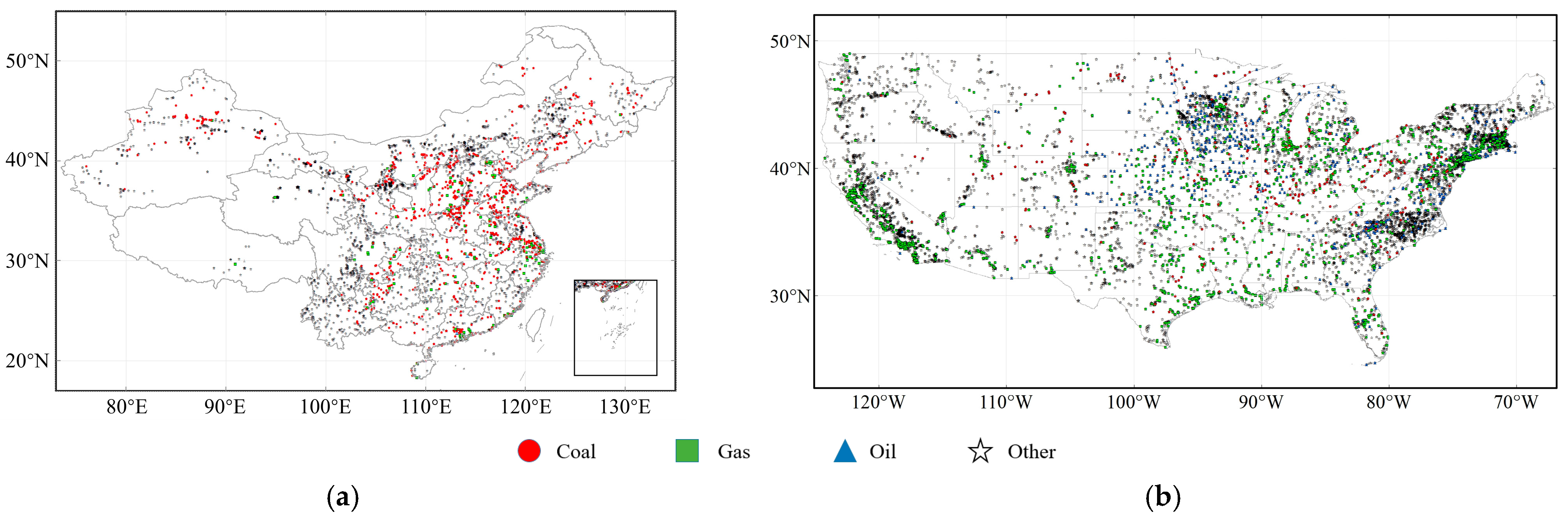
| Power Plant Data | The Global Power Plant Database | -/point | 2021 | World Resources Institute https://datasets.wri.org/datasets/global-power-plant-database (accessed on 16 October 2024) |
| Response Relationship (R2) | China | United States | ||
|---|---|---|---|---|
| ODIAC | EDGAR | ODIAC | EDGAR | |
| Grid-based | 0.42 | 0.46 | 0.44 | 0.44 |
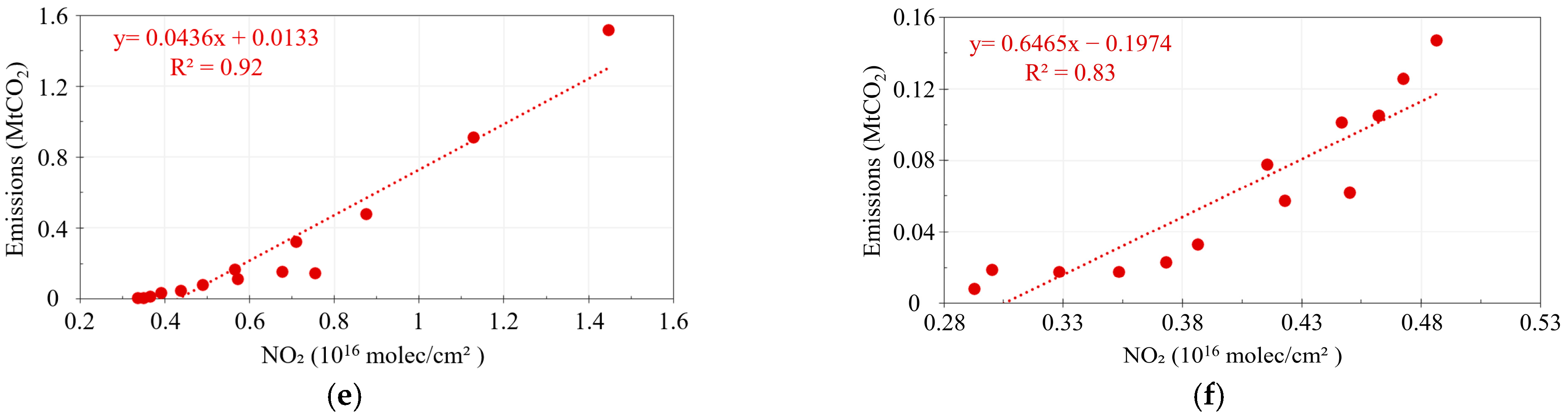
| Cluster-based | 0.92 | 0.92 | 0.82 | 0.83 |
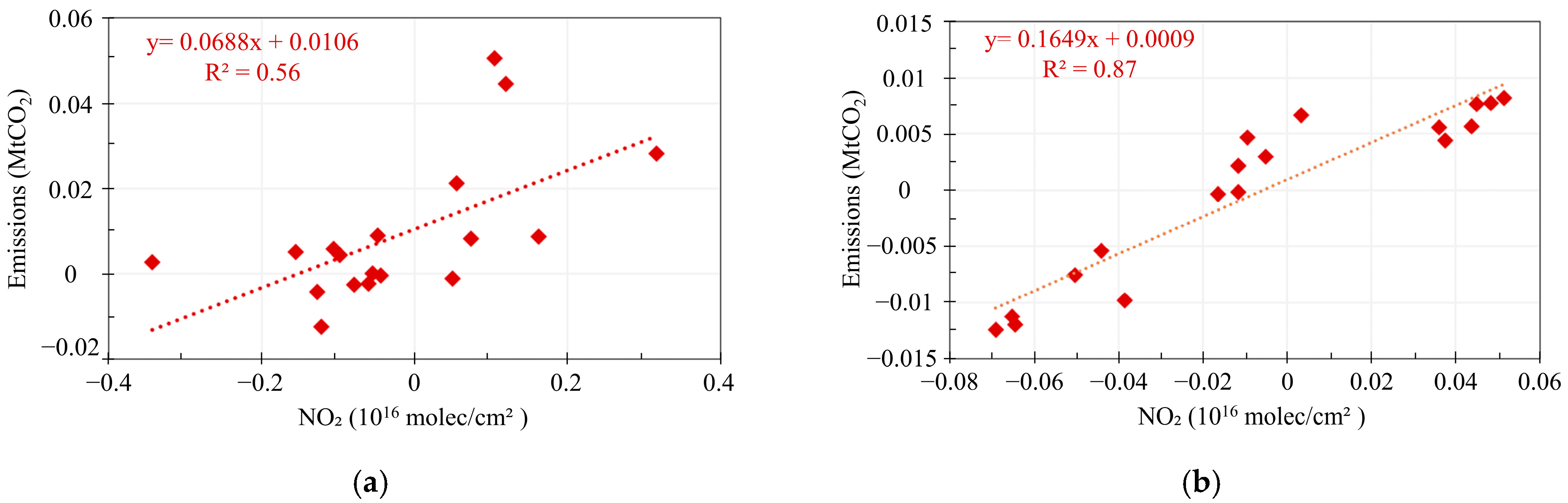
| In high-pollution areas | 0.36 | 0.56 | 0.53 | 0.87 |
Disclaimer/Publisher’s Note: The statements, opinions and data contained in all publications are solely those of the individual author(s) and contributor(s) and not of MDPI and/or the editor(s). MDPI and/or the editor(s) disclaim responsibility for any injury to people or property resulting from any ideas, methods, instructions or products referred to in the content. |
© 2025 by the authors. Licensee MDPI, Basel, Switzerland. This article is an open access article distributed under the terms and conditions of the Creative Commons Attribution (CC BY) license (https://creativecommons.org/licenses/by/4.0/).
Share and Cite
Guo, K.; Lei, L.; Song, H.; Ji, Z.; Liu, L. Co-Response of Atmospheric NO2 and CO2 Concentrations from Satellites Observations of Anthropogenic CO2 Emissions for Assessing the Synergistic Effects of Pollution and Carbon Reduction. Remote Sens. 2025, 17, 739. https://doi.org/10.3390/rs17050739
Guo K, Lei L, Song H, Ji Z, Liu L. Co-Response of Atmospheric NO2 and CO2 Concentrations from Satellites Observations of Anthropogenic CO2 Emissions for Assessing the Synergistic Effects of Pollution and Carbon Reduction. Remote Sensing. 2025; 17(5):739. https://doi.org/10.3390/rs17050739
Chicago/Turabian StyleGuo, Kaiyuan, Liping Lei, Hao Song, Zhanghui Ji, and Liangyun Liu. 2025. "Co-Response of Atmospheric NO2 and CO2 Concentrations from Satellites Observations of Anthropogenic CO2 Emissions for Assessing the Synergistic Effects of Pollution and Carbon Reduction" Remote Sensing 17, no. 5: 739. https://doi.org/10.3390/rs17050739
APA StyleGuo, K., Lei, L., Song, H., Ji, Z., & Liu, L. (2025). Co-Response of Atmospheric NO2 and CO2 Concentrations from Satellites Observations of Anthropogenic CO2 Emissions for Assessing the Synergistic Effects of Pollution and Carbon Reduction. Remote Sensing, 17(5), 739. https://doi.org/10.3390/rs17050739