High-Precision Localization Tracking and Motion State Estimation of Ground-Based Moving Target Utilizing Unmanned Aerial Vehicle High-Altitude Reconnaissance

Abstract

This paper focuses on the problem of ground-motion target localization tracking and motion state estimation for high-altitude reconnaissance using fixed-wing UAVs. Our goal is to accurately locate and track ground-moving targets and estimate their motion using visible light images, laser measurements of distance, and UAV position and attitude information. Firstly, this paper uses the target detection model of YOLOv8 to obtain the target pixel positions, combined with the measurement data, to establish the geolocalization model of the ground-motion target. Secondly, a motion state estimation algorithm with hierarchical filtering is proposed, and this algorithm performs motion state estimation for optoelectronic loads and ground-motion targets separately. Using the laser range sensor measurements as constraints, the optoelectronic load angle state quantities are involved together in estimating the ground target motion state, resulting in improved accuracy of ground-motion target localization tracking and motion state estimation. The experimental data show that the UAV ground-motion target localization tracking and motion estimation algorithm using hierarchical filtering reduces the localization tracking error by at least 7.5 m and the motion state estimation error by at least 0.8 m/s compared to other algorithms.

1. Introduction

With the development of computer vision, multi-sensor fusion, and other technologies, UAVs carrying a wide variety of sensors or tools are widely used in the fields of surveillance and rescue, surveying and mapping, military operations, and so on due to the advantages of low cost, reliability, and efficiency [1,2,3]. The ground target localization tracking and motion state estimation capabilities of vision sensor-equipped UAV systems are crucial during mission execution [4,5]. We aim to utilize UAV aerial images, laser measurement distance, UAV position, and attitude information to accurately locate and track ground-moving targets and estimate their motion states. The task of target localization tracking and motion state estimation can be divided into two steps: the first step is to identify target objects within the field of view using computer vision techniques. The second step is to locate and track the recognized object and estimate its motion state [6,7]. The ground target localization tracking and motion state estimation require the pixel coordinates of the ground target detected and identified in the UAV aerial image as a priori information.

Target recognition tasks can be categorized into large and small targets based on the size of the target object or its proximity to the vision sensor. In real-world ground target localization tracking, long-range targets of hundreds of meters contain only a few appearance features, which makes aerial small-target recognition challenging [8,9]. Since the YOLO family of models was proposed in 2016, it has become a mainstream method for target recognition due to its low latency and high detection accuracy [10,11,12,13]. ReDet and S²A-Net have become the most popular rotating target detection models in aerial image detection in recent years [14,15]. However, in our scenario, the exact rotation direction of the target is not required as a priori information. With limited arithmetic power, redundant rotation detection will affect the algorithm’s efficiency. In fixed-wing UAV high-altitude reconnaissance scenarios, Zhang et al. [16] propose an algorithm for detecting small targets in UAV aerial photography scenarios (HSP-YOLOv8). The engineered and improved HSP-YOLOv8 runs on a single-board Raspberry Pi 5.

The relative height or relative distance between the UAV and the ground target is necessary to realize the ground target localization and tracking. Lightweight UAS typically use accurate digital elevation models (DEMs) to obtain the relative height of the UAV to a ground target [17,18]. Alternatively, the relative distance between the UAV and the ground target is estimated based on a known target size combined with imaging principles [19,20]. Zhang et al. [21] proposed a method to estimate the relative height between the UAV and target without using a priori information, but it is only applicable when the ground target is in a stationary state. The further away the UAV is from the ground target, the more difficult it is to estimate the relative distance and relative height, and the accuracy of localization and tracking of long-distance targets will decrease dramatically [22]. An alternative solution is utilizing the distributed predictive visual servo control of UAV clusters [23] to acquire ground target images from multiple angles simultaneously and then use multi-view geometry for the 3D localization tracking of ground-moving targets [24]. However, it brings new problems with increased cost scale, cooperative control, and data synchronization difficulties [25].

When using UAV high-altitude reconnaissance for ground target localization tracking and motion state estimation, a typical mission scenario is that the UAV flies around the ground target at a high altitude. When the ground target appears in the field of view, the electrooptical stabilization and tracking platform (EOSTP) is controlled to lock onto and track the ground target, keeping the target in the center of the field of view [26] and using a laser ranging sensor to obtain the relative distance between the UAV and the target [27,28]. In complex outdoor environments, small angular deviations of the visual sensors due to the motion of the optoelectronic payload platform, unstable vibration, etc., can exacerbate the final localization error [29]. An attitude angle compensation approach has been used to improve the accuracy of ground target localization tracking. However, it does not take the irregular motion of the optoelectronic payload platform into account [30]. A dynamic target localization tracking and motion state estimation algorithm based on extended Kalman filtering is proposed in the reference [31]. The real-time estimation of ground-motion target position and motion state is combined with the trajectory smoothing algorithm to optimize the tracking trajectory, but the accuracy improvement is marginal.

In this study, we develop a framework for high-precision localization tracking and motion state estimation of ground-motion targets using high-altitude reconnaissance by UAVs, and the constructed system is shown in Figure 1. The main contributions of this paper are as follows:

• A new framework for the geolocalization of ground-moving targets based on monocular vision and laser range sensors is proposed. Using the laser ranging sensor to continuously measure the center point of the field of view, there is no need to align with the ground target and only a need to keep the ground target within the field of view of the UAV to complete the high-precision geolocalization tracking. It should be noted that the closer the ground target is to the center of the field of view, the higher the ground target positioning accuracy.
• The first layer of the layered filtering algorithm estimates the motion state of the optoelectronic load, and the second layer of the filtering estimates the motion state of the ground target. The first layer filter compensates for the error of the AHRS data to a certain extent, which may reach more than a degree, thus seriously affecting the tracking accuracy of the UAV on the ground dynamic target [32]. The second layer of filtering is constrained by the laser ranging value, which greatly improves the estimation accuracy of the ground target motion state.

2. Ground Dynamic Target Geolocalization Model

2.1. Relevant Research Base

In our previous related work [33], we derived in detail the transformation relationship between the geographic coordinate system and the spatial Cartesian coordinate system. In this paper, the position $t_u={(x_u,y_u,z_u)}^T$ of the UAV under the spatial Cartesian coordinate system can be obtained from the GPS. At the same time, according to the laser ranging, we can know that the corresponding point of the image center on the ground is represented in the camera coordinate system as follows: $t_s={(\mathrm{0,0},L)}^T$, where $L$ is the distance to the center of the field of view as measured by the laser ranging equipment of the optronic pod. The coordinate transformation relationship between the ground point corresponding to the center of the image in the spatial Cartesian coordinate system and the camera coordinate system is as follows:

$$t_s=C_u^v\cdot C_b^u\cdot (t_e-t_u)$$

(1)

In this equation, $C_b^u=C_x\left(\gamma \right){·C}_y\left(\theta \right){·C}_z\left(\phi \right)$, the UAV navigational yaw angle is φ, the UAV navigational pitch angle is γ, and the UAV navigational roll angle is θ. $C_x(·)$, $C_y(·)$ and $C_z(·)$ are rotation matrices about the X-axis, Y-axis, and Z-axis, respectively. $C_u^v=C_x\left(\beta \right){·C}_y(-180°){·C}_z(180°-\alpha )$, where α is the azimuth of rotation of the photoelectric load, and β is the optoelectronic load pitch angle. The coordinates of the ground point correspond to the center of the image in the spatial Cartesian coordinate system $t_e={(x_e,y_e,z_e)}^T$. The computational expression can be written as

$$t_e={(C_b^u)}^{-1}\cdot {(C_u^v)}^{-1}\cdot t_s+t_u$$

(2)

According to (2), the coordinates of the ground point corresponding to the center of the field of view under the spatial right-angle coordinate system can be obtained and then converted to the geographic coordinate system of the Earth; the latitude, longitude, and altitude of the ground point corresponding to the center of the field of view can be obtained.

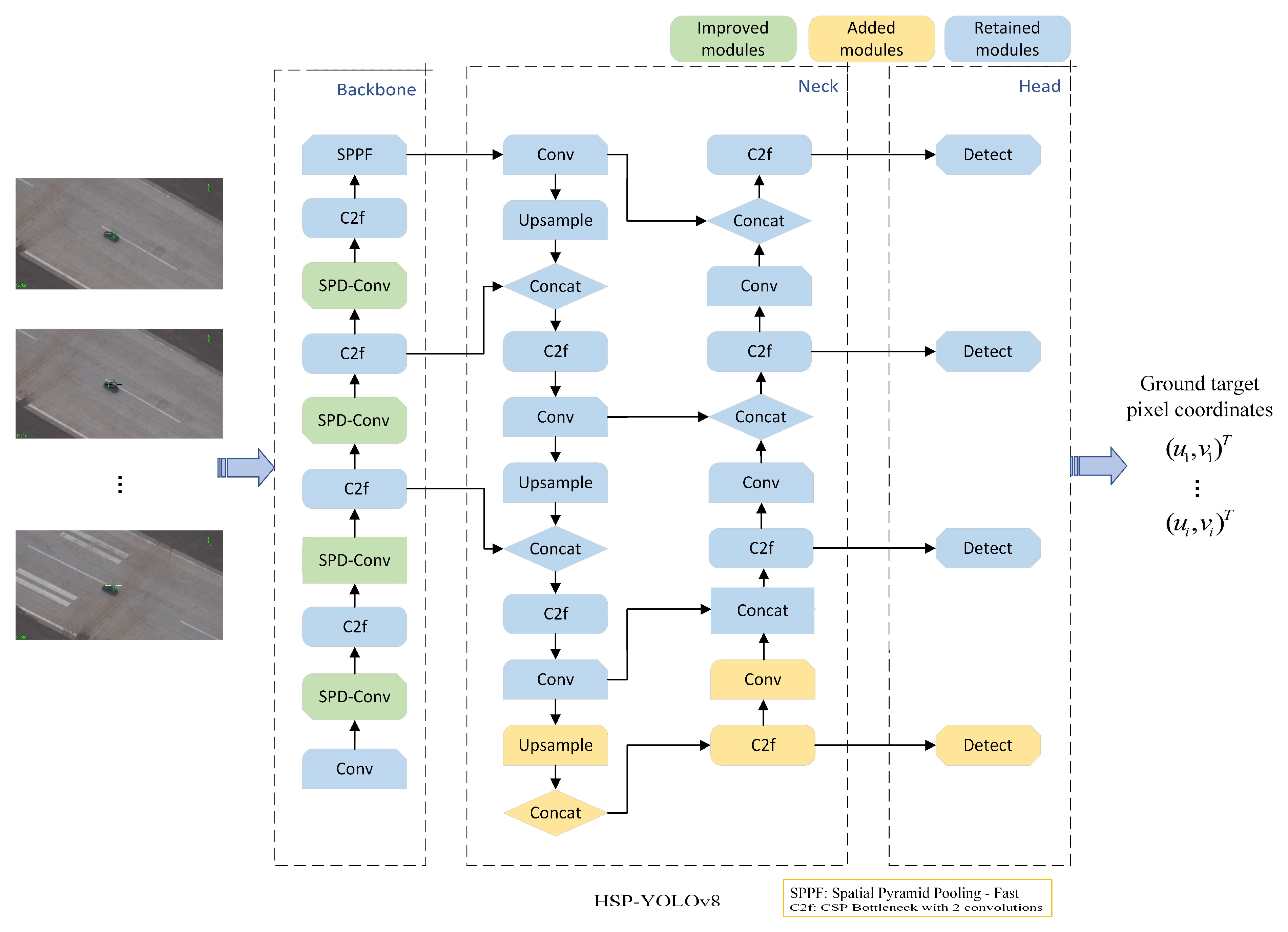
Our goal is geolocalization and tracking targets within the field of view, and to achieve this goal, we also need to use our previous related research [16]. We added an extra tiny prediction head and a null-depth convolution module to the YOLOv8 algorithm and a post-processing algorithm more suitable for small target recognition, the Space-to-Depth Convolution (SPD-Conv) module. In the fixed-wing UAV high-altitude reconnaissance scenario, the network structure that has been specially designed by us runs on a single-board Raspberry Pi 5, and the algorithm has a speed of 5 FPS, which is consistent with the laser measurement distance frequency. The input and output of the algorithm and the network structure are shown in Figure 2. In this paper, we default to the target pixel location in the UAV vision image being accessible, and we do not discuss the case where the target pixel location is not accessible due to image quality.

2.2. Geolocalization of Any Point in an Image

The geolocation of an arbitrary point in an image differs from the geolocation of the center of the image. Because of the lack of physical distance measured by laser ranging at the target point, it is impossible to directly obtain the coordinates of the target point in the camera coordinate system. Therefore, it is necessary to calculate the coordinates of the ground position at the target point in the camera coordinate system, and then the coordinates of the target point in the geographic coordinate system can be obtained after coordinate conversion.

In the camera coordinate system, the two-dimensional coordinates of any point $m$ in the image are expressed as ${(x_m,y_m)}^T$. Point $M$ is the corresponding point of point $m$ in the physical plane. The geometric relationship between the coordinates of point $M$ under the camera coordinate system ${(x_M,y_M,z_M)}^T$ and the pixel coordinates ${(u,v)}^T$ of point m to each other can be expressed as follows:

$$\left\{\begin{array}{c}{x}_m\cdot z_M=x_M\cdot F\\ y_m\cdot z_M=y_M\cdot F\\ x_m=l_x\cdot \left(u-c_x\right)\\ y_m=l_y\cdot \left(v-c_y\right)\end{array}\right.$$

(3)

In this equation, $F$ is the focal length of the camera mounted on the drone. ${(c_x,c_y)}^T$ are the pixel coordinates of the center point of the image, and $l_x$ and $l_y$ are the horizontal and vertical physical lengths represented by each camera pixel, respectively.

The geometric relationship of imaging during UAV high-altitude reconnaissance is shown in Figure 3. The plane $X_0{C}_0{Y}_0$ indicates the ground taken during aerial photography. $XCY$ represents the plane that is imaged inside the camera when the camera is imaging. In plane $XCY$, $C$ is the center of the camera’s field of view, and the length of $\mathrm{O}C$ is the focal length $F$. $CX$ denotes the horizontal axis of the $XCY$-plane. $CY$ represents the vertical axis of the plane $XCY$. Point $M$ is the corresponding point of point $m,$ the corresponding point of the projection onto the ground. In plane $X_0{C}_0{Y}_0$, $C_0$ is the intersection of the centerline of the camera’s field of view and the plane $X_0{C}_0{Y}_0$. $C_0{X}_0$ is the projection of the $CX$-axis through $C_0$ in the plane $X_0{C}_0{Y}_0$. $C_0{Y}_0$ is the mapping of the $CY$-axis in the plane $X_0{C}_0{Y}_0$. $O_{\mathrm{g}}$ is the point under the projection of $O$ in the plane $X_0{C}_0{Y}_0$. $O{X}_{\mathrm{v}}{C}_{\mathrm{v}}{Y}_{\mathrm{v}}$ denotes the camera coordinate system. $O{X}_{\mathrm{b}}{C}_{\mathrm{b}}{Y}_{\mathrm{b}}$ represents a system of right-angled coordinates in space.

The angle between $\overrightarrow{OC}$ and $Z_{\mathrm{b}}$-axis is noted as λ. The angle between $\overrightarrow{Om}$ and $\overrightarrow{OC}$ is noted as μ. The angle between $\overrightarrow{Om}$ and $Z_{\mathrm{b}}$-axis is noted as ω. Vector $\overrightarrow{OC}={(\mathrm{0,0},1)}^T$ is the vector in the camera coordinate system $O{X}_{\mathrm{V}}{Y}_{\mathrm{V}}{Z}_{\mathrm{V}}$. The unit vector of the $Z_{\mathrm{b}}$-axis of the coordinate system $O{X}_{\mathrm{b}}{Y}_{\mathrm{b}}{Z}_{\mathrm{b}}$ is $\overrightarrow{e_b}={(\mathrm{0,0},-1)}^T$. $\overrightarrow{OC}$ is represented in the coordinate system $O{X}_{\mathrm{b}}{Y}_{\mathrm{b}}{Z}_{\mathrm{b}}$ as $\overrightarrow{a}$, so $\overrightarrow{a}=C_u^b{C}_v^u·\overrightarrow{OC}$. $\overrightarrow{Om}={(x_m,y_m,F)}^T$ is the vector in the camera coordinate system $O{X}_{\mathrm{V}}{Y}_{\mathrm{V}}{Z}_{\mathrm{V}}$. $\overrightarrow{Om}$ is represented in the coordinate system $O{X}_{\mathrm{b}}{Y}_{\mathrm{b}}{Z}_{\mathrm{b}}$ as $\overrightarrow{b}$. $\overrightarrow{b}=C_u^b{C}_v^u·\overrightarrow{Om}$, so the angle of pinch λ, μ, ω can be expressed as

$$\left\{\begin{array}{c}\lambda =\arccos {\displaystyle \frac{\overrightarrow{a}\cdot \overrightarrow{e_b}}{\left|\overrightarrow{a}\right|\cdot \left|\overrightarrow{e_b}\right|}}\\ \mu =\arccos {\displaystyle \frac{F}{\sqrt{x_m^2+y_m^2+F^2}}}\\ \omega =\arccos {\displaystyle \frac{\overrightarrow{b}\cdot \overrightarrow{e_b}}{\left|\overrightarrow{b}\right|\cdot \left|\overrightarrow{e_b}\right|}}\end{array}\right.$$

(4)

Let $O{C}_0=L$, then $H=L·\cos \lambda$, $\left|\overrightarrow{OM}\right|=H/\cos \omega$, and the $Z_{\mathrm{v}}$-axis coordinates of point $M$ in the camera coordinate system are

$$z_M=L\cdot \cos \mu \cdot \cos \lambda /\cos \omega =L\cdot \cos \lambda \cdot {\displaystyle \frac{F}{\cos \omega \sqrt{x_m^2+y_m^2+F^2}}}$$

(5)

Substituting into (3), the other coordinate values under the camera coordinates of the point $M$ can be calculated.

$$\left\{\begin{array}{c}{x}_M={\displaystyle \frac{x_m\cdot L\cdot \cos \lambda }{\cos \omega \cdot \sqrt{x_m^2+y_m^2+F^2}}}\\ y_M={\displaystyle \frac{y_m\cdot L\cdot \cos \lambda }{\cos \omega \cdot \sqrt{x_m^2+y_m^2+F^2}}}\end{array}\right.$$

(6)

At this point, we have obtained the coordinates of point $M$ in the camera coordinate system ${(x_M,y_M,z_M)}^T$, and then the coordinates of point $M$ under the coordinate system of the spatial Cartesian coordinate system can be calculated according to (2).

$$t_M={(C_b^u)}^{-1}\cdot {(C_u^v)}^{-1}\cdot {(x_M,y_M,z_M)}^T+t_u$$

(7)

Then, $t_M$ is converted to a geographic coordinate system, which completes the geolocalization of any point in the image.

3. Ground Dynamic Target Tracking Estimation Model

Considering that in practical applications, the rotational azimuth and pitch angle of the photoelectric load provided by the photoelectric imaging module have some deviation from the real values. Combined with other measurement errors, the calculated ground target position will also have a large error. The calculated ground target position jumps and changes at successive times. Such results do not match the real movement trajectory and are not favorable for practical applications. Therefore, it is necessary to establish a corresponding motion-tracking model to suppress the influence of various types of noise on the system by designing a suitable filtering-tracking algorithm to obtain more accurate and stable target-tracking results.

A typical discrete-time nonlinear state-space model and state-observation model can be expressed as follows:

$$\left\{\begin{array}{l}{\theta }_k=f({\theta }_{k-1})+s_k\hfill \\ m_k=h({\theta }_k)+o_k\hfill \end{array}\right.$$

(8)

where ${\mathsf{\theta }}_k\in {\mathbb{R}}^{\mathit{N}}$ and ${\mathbf{m}}_k\in {\mathbb{R}}^{\mathit{M}}$ denote the state vector and observation vector at the $k$ moment, respectively. $f\left(·\right)$ and $h\left(·\right)$ represent the nonlinear state function and observation function, respectively. ${\mathbf{s}}_k\in {\mathbb{R}}^{\mathit{N}}$ is a zero-mean Gaussian process noise satisfying ${\mathbf{s}}_k~\mathcal{N}(\mathbf{0},\mathbf{Q})$.${\mathbf{o}}_k\in {\mathbb{R}}^{\mathit{M}}$ is the zero-mean Gaussian measurement noise satisfying ${\mathbf{o}}_k~\mathcal{N}(\mathbf{0},\mathbf{R})$.

3.1. Optical Load Equation of Motion

For the motion of the photoelectric load carried by the UAV, the equation of motion of the photoelectric load can be constructed as

$${\theta }_{1,k}=f_1({\theta }_{1,k-1})+s_{1,k}=F_1{\theta }_{1,k-1}+s_{1,k}$$

(9)

The photoelectric load at the $k$ moment of real-time state is represented by vector ${\mathsf{\theta }}_{\mathbf{1}\mathbf{,}\mathit{k}}{=\left[{\alpha }_k,{\beta }_k,\dot{{\alpha }_k},\dot{{\beta }_k}\right]}^T$, representing the angle values and rotation speeds of the photoelectric load at the $k$ moment and the angular values and rotation speeds of the photoelectric load in the rotational and pitching directions, respectively. Thus, the state transfer matrix ${\mathbf{F}}_1$ can be written as

$$F_1=\left[\begin{array}{cccc}1& 0& \Delta t& 0\\ 0& 1& 0& \Delta t\\ 0& 0& 1& 0\\ 0& 0& 0& 1\end{array}\right]$$

(10)

The results of drone vibration, wind, and other effects can be modeled by noise ${\mathbf{s}}_{1,k}$. For the convenience of model solving, it is assumed that noise ${\mathbf{s}}_{1,k}$ approximately follows a Gaussian distribution, ${\mathbf{s}}_{1,k}\in {\mathbb{R}}^4$.

3.2. Dynamic Target Equations of Motion

For the motion trajectory tracking of a ground-motion target, the motion equation of the target can be constructed as

$${\theta }_{2,k}=f_2({\theta }_{2,k-1})+s_{2,k}=F_2{\theta }_{2,k-1}+s_{2,k}$$

(11)

The real-time state at the moment $k$ of a ground-moving target is represented by the vector ${\mathsf{\theta }}_{\mathbf{2}\mathbf{,}\mathit{k}}{=\left[x_k,y_k,z_k,\dot{x_k},\dot{y_k},\dot{z_k}\right]}^T$, representing, respectively, the ground-motion target coordinates and velocities in the $x$, $y,$ and $z$ directions of the reference coordinate system at moment $k$. Thus, the state transfer matrix ${\mathbf{F}}_2$ can be written as

$$F_2=\left[\begin{array}{llllll}1\hfill & 0\hfill & 0\hfill & \Delta t\hfill & 0\hfill & 0\hfill \\ 0\hfill & 1\hfill & 0\hfill & 0\hfill & \Delta t\hfill & 0\hfill \\ 0\hfill & 0\hfill & 1\hfill & 0\hfill & 0\hfill & \Delta t\hfill \\ 0\hfill & 0\hfill & 0\hfill & 1\hfill & 0\hfill & 0\hfill \\ 0\hfill & 0\hfill & 0\hfill & 0\hfill & 1\hfill & 0\hfill \\ 0\hfill & 0\hfill & 0\hfill & 0\hfill & 0\hfill & 1\hfill \end{array}\right]$$

(12)

The results of ground, wind, and other effects in the environment in which a ground-moving target is located can be modeled by noise ${\mathbf{s}}_{2,k}$. For the convenience of model solving, it is assumed that noise ${\mathbf{s}}_{2,k}$ approximately follows a Gaussian distribution, ${\mathbf{s}}_{2,k}\in {\mathbb{R}}^6$.

3.3. Constructing the Observation Equation

For photoelectric loads, the observation equation can be written as

$$\left[\begin{array}{c}{m}_{\alpha ,k}\\ m_{\beta ,k}\end{array}\right]=h_1({\theta }_{1,k})+o_{1,k}=\left[\begin{array}{c}{\alpha }_k\\ {\beta }_k\end{array}\right]+o_{1,k}$$

(13)

where ${\mathbf{m}}_{1,k}{=\left[m_{\alpha ,k},m_{\beta ,k}\right]}^T$ represents the measured value obtained by the system through the sensor at moment $k$, $m_{\alpha ,k}$ is the rotational azimuth, and $m_{\beta ,k}$ is the pitch angle. Units are in the international system of units. Considering that this result is affected by sensor noise and has some deviations from the true value, it is modeled using the measurement noise ${\mathbf{o}}_{1,k}$. For the convenience of model solving, it is assumed that the measurement noise ${\mathbf{o}}_{1,k}$ approximately follows a Gaussian distribution, and ${\mathbf{o}}_{1,k}\in {\mathbb{R}}^2$.

For dynamic targets on the ground, the distance between the UAV and the ground point corresponding to the center of the field of view can be obtained from the laser ranging sensor, which, in terms of $d_k,$ can be written as

$$d_k=\sqrt{{\left(x_{u,k}-x_{c,k}\right)}^2+{\left(y_{u,k}-y_{c,k}\right)}^2+{\left(z_{u,k}-z_{c,k}\right)}^2}$$

(14)

where ${(x_{u,k},y_{u,k},z_{u,k})}^T$ denotes the coordinates of the UAV’s location at moment $k$, and ${(x_{c,k},y_{c,k},z_{c,k})}^T$ denotes the coordinates of the center of the visual field corresponding to the ground point at moment $k$. The observation equation can be written as

$$\left[\begin{array}{c}{m}_{x,k}\\ m_{y,k}\\ m_{z,k}\\ m_{d,k}\end{array}\right]=h_2({\theta }_{2,k})+o_{2,k}=\left[\begin{array}{c}{x}_k\\ y_k\\ z_k\\ d_k\end{array}\right]+o_{2,k}$$

(15)

where ${\mathbf{m}}_{2,k}{=\left[m_{x,k},m_{y,k},m_{z,k},m_{d,k}\right]}^T$ indicates the results of the initial calculation of the ground target position by the system at moment $k$ through (7) and the measured value of the laser ranging sensor, all in the international system of units. The measured values are affected by sensor noise and deviate from the true values, which are modeled using measurement noise ${\mathbf{o}}_{1,k}$. For the convenience of model solving, the noise ${\mathbf{o}}_{1,k}$ is considered to follow a Gaussian distribution, ${\mathbf{o}}_{2,k}\in {\mathbb{R}}^4$.

3.4. Algorithm Iteration Process

The iterative process of the algorithm in this paper consists of two steps: Propagation and Updating. At the Propagation step, based on the estimation of the target state $〈{\mathsf{\theta }}_{k-1}〉$ and the corresponding estimation error covariance ${\mathsf{\Sigma }}_{k-1}$ at moment $k-1$, the prediction of the target state ${\mathit{\theta }}_k^{\prime }$ and the corresponding prediction error covariance ${\mathsf{\Sigma }}_k^{\prime }$ at moment $k$ is accomplished, and the specific process is expressed as follows:

$${\theta }_k^{\prime }=f(〈{\theta }_{k-1}〉)$$

(16)

$${\Sigma }_k^{\prime }=F{\Sigma }_{k-1}{F}^T+Q$$

(17)

At the Update step, the predicted values are first utilized to compute the Jacobi matrix ${\mathbf{H}}_k$, which is used to compute the Kalman gain ${\mathbf{K}}_k$. Then, the predicted value ${\mathit{\theta }}_k^{\prime }$ is corrected based on the measured value ${\mathbf{m}}_k$ provided by the platform to obtain an estimate $〈{\mathsf{\theta }}_k〉$ of the target state at moment $k$. Finally, the error covariance matrix ${\mathsf{\Sigma }}_k$ of this estimate is calculated, and the procedure is expressed as follows:

$${H_k=\left.{\displaystyle \frac{\partial h(\theta )}{\partial \theta }}\right|}_{\theta ={\theta }_k^{\prime }}$$

(18)

$$K_k={\Sigma }_k^{\prime }{H}_k^T{\left(H_k{\Sigma }_k^{\prime }{H}_k^T+R\right)}^{-1}$$

(19)

$$〈{\theta }_k〉={\theta }_k^{\prime }+K_k\left[m_k-h({\theta }_k^{\prime })\right]$$

(20)

$${\Sigma }_k=\left(I-K_k{H}_k\right){\Sigma }_k^{\prime }$$

(21)

This completes the estimation of the ground target state at moment $k$. Afterwards, whenever the measurements ${\mathbf{m}}_{k+1}$ at moment $k+1$ are obtained, the ground target state estimation at moment $k+1$ can be performed. By recursively proceeding in this manner, a real-time estimation of the target state is achieved.

Such an iterative approach fully utilizes the available historical observations to predict the current state of the ground target. Compared with the direct use of observations to estimate the ground target state, our hierarchical filtering algorithm utilizes more a priori information by first estimating the current motion state of the optoelectronic load and then using the updated angular data of the optoelectronic load to participate in the estimation of the current state of the ground target so that we can obtain more accurate and stable results of the ground target positioning and tracking and the motion state estimation.

4. Results and Discussion

In the previous two sections, we introduced a hierarchical filtering algorithm for the high-precision geolocalization tracking and motion state estimation of UAV dynamic targets. In this section, we evaluate the performance of our proposed algorithm, HPLTMSE, in all aspects and compare the algorithms EKF, VOLTS [31], and MGG [30]. We set up three separate sets of experiments to verify. The ground target in the test moves in three different motion modes, and we use an ASN-216 fixed-wing UAV to conduct aerial following reconnaissance of the target and collect real-time UAV visual images, UAV position, UAV attitude, optoelectronic load attitude, and laser ranging values. The experiment site is shown in Figure 4. The experiment site is located at the geographical coordinates (108°51′22″E, 37°45′26″N) of an airport in the northern region of Shaanxi Province. At the same time, the GPS receiver mounted on the ground target provides us with real-time position and velocity information of the ground target as the real values for algorithmic comparison.

The experiments simulate three scenarios for military applications. Experiment A simulates the tracking and positioning of transportation vehicles with high-speed maneuverability in variable-acceleration linear motion. Experiment B simulates the tracking and positioning of transport vehicles with high-speed maneuverability in a variable-acceleration folding motion. Experiment C simulates the tracking and positioning of an armored vehicle with slightly weaker maneuverability. However, the armored vehicle will change its maneuvering state to be towed by the transport vehicle in the course of the mission, so there will be two variable-acceleration motions. The algorithm was developed and tested on a PC but ultimately runs on a single-board Raspberry Pi 5, and the errors of each sensor of the drone platform are shown in

Table 1. Error of each sensor of the UAV platform.

Parameter Name	Error Value
UAV navigational yaw angle/°	1
UAV navigational pitch angle/°	0.2
UAV navigational roll angle/°	0.2
Optoelectronic load pitch angle/°	0.2
Optoelectronic load rotation angle/°	0.2
UAV GPS/m	10
Laser measurement distance/m	10

.

4.1. Experiment A

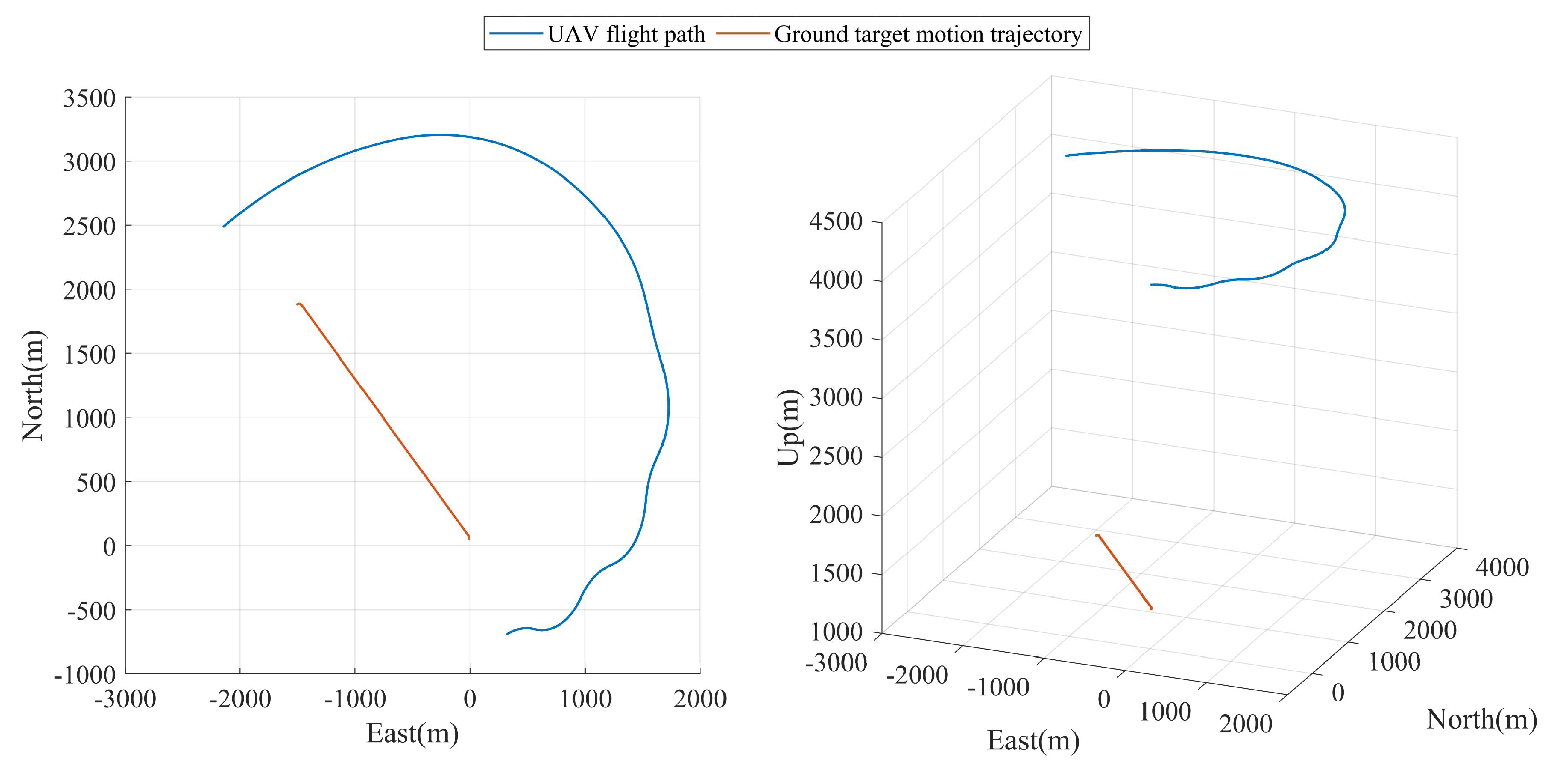
In experiment A, the ground-motion target moved along a closed section of road in a straight-line, variable-speed motion, accelerating from about 20 km/h to about 70 km/h and decelerating to about 20 km/h. At the same time, the UAVs circled around the ground target at distances ranging from 3850 m to 4550 m and collected the required data. The UAV flight trajectory and ground target movement trajectory are shown in Figure 5. The laser measurement distance is shown in Figure 6. The EKF, VOLTS, and MGG algorithms are used for the geolocalization tracking and motion state estimation of ground-motion targets on the first set of UAV time-series data collected, respectively, to compare and verify the performance of the HPLTMSE algorithm proposed in this paper.

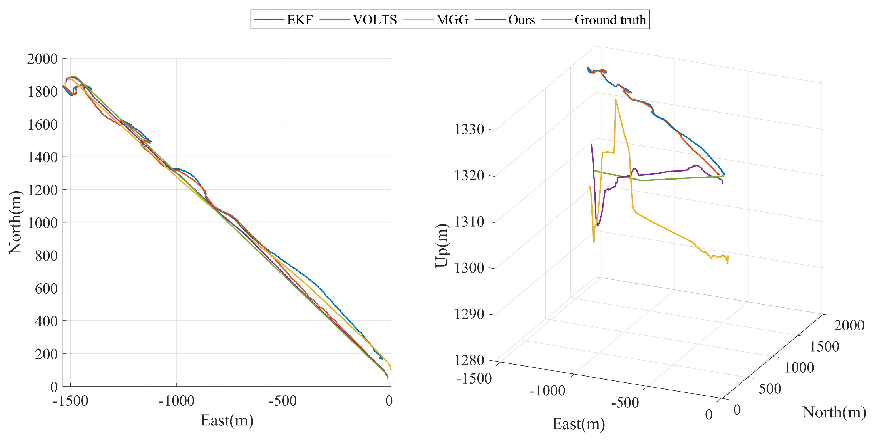
The geolocalization tracking results of the four algorithms for ground-motion targets in experiment A are shown in Figure 7. From the figure, it can be seen that among the two-dimensional trajectories in the horizontal plane output by the four algorithms, HPLTMSE most closely matches the real motion trajectory of the ground target, MGG is a little bit worse, and VOLTS and EKF have the worst performance in terms of accuracy. This is because VOLTS is essentially an EKF superimposed trajectory smoothing algorithm. The EKF algorithm is effective only for Gaussian-distributed noise and is not robust to non-Gaussian-distributed noise. This is manifested by the fact that when the sensor measurements appear to deviate from the wild values of the expected point cloud, the estimation results given by the system will have large jumps and will not be stable enough. In comparison, MGG is based on UAV visual images, and HPLTMSE is based on hierarchical filtering and laser-measured distance constraints, which enable the geolocalization of ground targets and smoother trajectory tracking as long as the ground targets are not lost in the UAV’s field of view. The accuracy of the HPLTMSE algorithm for estimating ground target height information is significantly improved due to the laser measurement distance constraints.

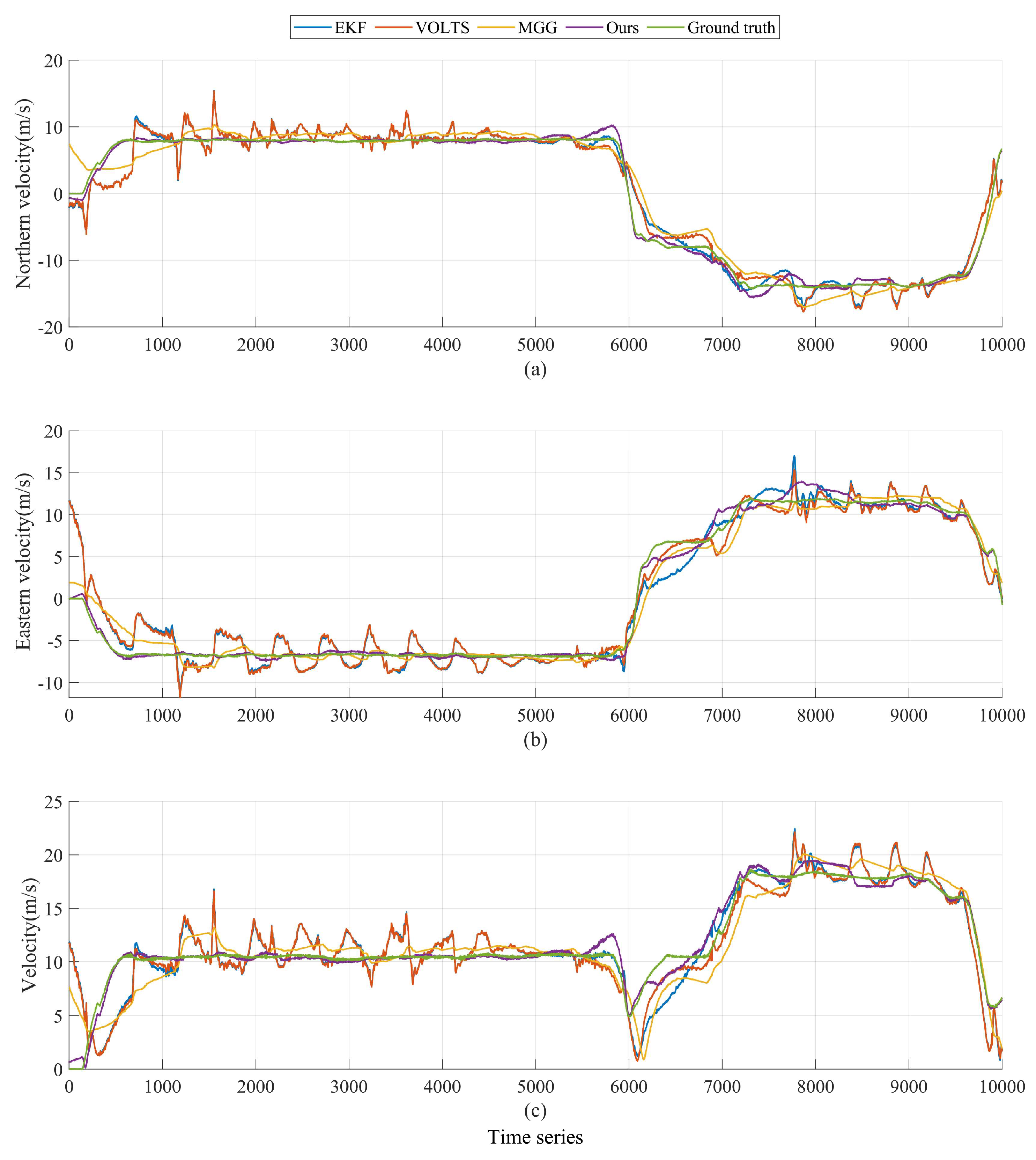
The results of the ground target motion state estimation for experiment A are shown in Figure 8. From the figure, it can be seen that the purple curve is closest to the green curve when the motion speed of the ground target changes, i.e., the HPLTMSE algorithm has the fastest response to the motion state estimation of the ground target among the four algorithms. The VOLTS and EKF algorithms are subject to large fluctuation distortions in ground target motion state estimation due to the poor performance of the results of the geolocalization and tracking of ground targets.

The error metrics (RMSE) for each of the four algorithms in experiment A are shown in

Table 2. The error metrics (RMSE) for each of the four algorithms in experiment A.

		EKF	VOLTS	MGG	Ours
Localization tracking	Confidence interval (90% confidence level)	[17.78,90.20]	[22.59,76.99]	[22.69,48.05]	[10.12,32.10]
	Combined error (m)	46.82	46.7	37.21	22.26
	Up (m)	14.04	14.02	12.83	3.34
Motion state estimation	Northern velocity (m/s)	2.19	2.14	1.93	0.99
	Eastern velocity (m/s)	2.28	2.49	2.06	0.88
	Velocity (m/s)	2.61	2.4	2.16	1.13

. Benefiting from the laser measurement distance constraints, the HPLTMSE algorithm significantly improves the estimation accuracy of the ground target height information, with a ground target height estimation RMSE of 3.34 m. The overall RMSE of this paper’s algorithm ground target geolocalization and tracking is 22.26 m, and the estimated RMSE of the ground target motion velocity is 1.13 m/s. Compared with other comparative algorithms, this paper’s algorithm reduces the ground target geolocalization and tracking error by at least 14.95 m and reduces the estimation error of the ground target’s movement speed by at least 1.03 m/s.

4.2. Experiment B

In experiment B, the ground-motion target made a round-trip motion along a closed road, and the motion speed was decelerated from about 70 km/h to about 20 km/h and then accelerated to about 70 km/h again. At the same time, the UAV flew asymptotically at a distance of 4650 m from the ground target to a distance of 3900 m from the ground target to reconnoiter the ground target and collect the required data. The UAV flight trajectory and ground target movement trajectory are shown in Figure 9.

The laser measurement distance is shown in Figure 10. The EKF, VOLTS, and MGG algorithms are used for geolocalization tracking and the motion state estimation of ground-motion targets, respectively, on the second set of UAV time series data collected to compare and verify the performance of the HPLTMSE algorithm proposed in this paper.

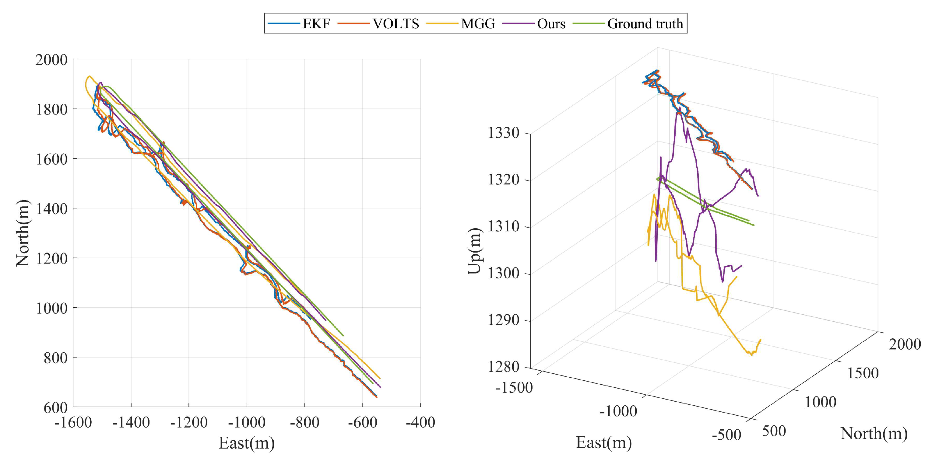
The geolocalization tracking results of the four algorithms for ground-motion targets in experiment B are shown in Figure 11, which are consistent with the experiment A results. From Figure 11, it can be seen that among the two-dimensional trajectories in the horizontal plane output by the four algorithms, HPLTMSE best fits the real motion trajectory of the ground target, MVBMTG is a little bit worse, and VOLTS and EKF perform the worst in terms of accuracy. It is worth noting that the MGG algorithm has a larger tracking trajectory error at this point when the ground target turns its direction due to the large changes in the UAV’s visual image and the increased difficulty in image alignment. As can be seen in Figure 11, the accuracy of the HPLTMSE algorithm in estimating the ground target height information is significantly better than the other comparative algorithms due to the constraint of the laser measurement distance.

The results of the ground target motion state estimation for experiment B are shown in Figure 12. From the figure, it can be seen that the purple curve is closest to the green curve when the ground target’s motion speed changes, i.e., the HPLTMSE algorithm has the fastest response to the ground target’s motion state estimation among the four algorithms. The VOLTS and EKF algorithms are subject to large fluctuation distortions in ground target motion state estimation due to the poor performance of the results of the geolocalization and tracking of ground targets.

The error metrics (RMSE) for each of the four algorithms in experiment B are shown in

Table 3. The error metrics (RMSE) for each of the four algorithms in experiment B.

		EKF	VOLTS	MGG	Ours
Localization tracking	Confidence interval (90% confidence level)	[20.62,78.62]	[23.71,76.34]	[13.69,64.17]	[10.04,37.22]
	Combined error (m)	66.66	59.98	41.38	25.31
	Up (m)	17.82	17.83	17.02	8.42
Motion state estimation	Northern velocity (m/s)	2.7	2.59	2.35	1.19
	Eastern velocity (m/s)	2.34	2.15	1.92	1.04
	Velocity (m/s)	3.19	2.93	2.45	1.39

. Benefiting from the laser measurement distance constraint, the HPLTMSE algorithm significantly improves the estimation accuracy of ground target height information. The overall RMSE of this paper’s algorithm ground target geolocalization and tracking is 25.31 m. The estimated RMSE of the ground target height is 8.42 m. The estimated RMSE of the ground target motion velocity is 1.39 m/s. Compared with other comparative algorithms, this paper’s algorithm reduces the geolocalization and tracking error of ground targets by at least 16.07 m and reduces the estimation error of ground targets’ movement speed by at least 1.06 m/s.

4.3. Experiment C

In experiment C, the ground-motion target made a folding back for one lap motion along a section of a closed road, with a speed of about 35 km/h for the first half of the motion from rest and about 65 km/h for the second half of the motion. At the same time, the UAV flew asymptotically at a distance of 5300 m from the ground target to 3600 m from the ground target to transform into an encircling flight to reconnoiter the ground target and collect the required data. The UAV flight trajectory and ground target movement trajectory are shown in Figure 13. The laser measurement distance is shown in Figure 14. The EKF, VOLTS, and MGG algorithms are used for geolocalization tracking and the motion state estimation of ground-motion targets for the third set of UAV time series data collected, respectively, to compare and verify the performance of the HPLTMSE algorithm proposed in this paper.

The geolocalization tracking results of the four algorithms for ground-motion targets in experiment C are shown in Figure 15. The results of ground target motion state estimation in experiment C are shown in Figure 16. Consistent with the results of experiment A and experiment B, it can be seen from the figure that among the tracking trajectories output by the four algorithms, HPLTMSE most closely matches the real trajectory of the ground target, MGG is a little bit worse, and the accuracy of VOLTS and EKF is the worst. Among the four algorithms, the HPLTMSE algorithm estimates the ground target’s motion state most accurately, and the algorithm performs best when the ground target’s motion state is stable.

The error metrics (RMSE) for each of the four algorithms in experiment C are shown in

Table 4. The error metrics (RMSE) for each of the four algorithms in experiment C.

		EKF	VOLTS	MGG	Ours
Localization tracking	Confidence interval (90% confidence level)	[2.31,70.82]	[4.12,69.03]	[2.29,58.54]	[3.70,40.41]
	Combined error (m)	37.43	36.97	34.92	26.99
	Up (m)	13.68	13.65	13.18	5.84
Motion state estimation	Northern velocity (m/s)	1.89	1.91	1.92	1.03
	Eastern velocity (m/s)	2.12	1.96	1.32	1.01
	Velocity (m/s)	2.22	2.14	1.91	1.08

. Benefiting from the laser measurement distance constraint, the accuracy of the HPLTMSE algorithm in estimating the ground target height information is significantly improved, and the RMSE of the ground target height estimation is 5.84 m. The overall RMSE of this paper’s algorithm for ground target geolocalization and tracking is 26.99 m, and the RMSE of ground target motion velocity estimation is 1.08 m/s. Compared with other comparative algorithms, this paper’s algorithm reduces the ground target geolocalization and tracking error by at least 7.93 m and the ground target motion velocity estimation error by at least 0.83 m/s.

5. Conclusions

In this work, we propose a framework for the geolocalization tracking and motion state estimation of ground-motion targets based on monocular vision and laser ranging sensors. Based on the pixel position information of ground targets in UAV aerial images that have been obtained, a general formula for the geolocalization of ground targets in the field of view under non-directed laser irradiation is derived. We designed a hierarchical filtered motion state estimation algorithm to estimate the motion states of optoelectronic loads and ground targets separately. The laser measurement distance is used as a constraint to participate in the estimation of the ground target motion state using the first layer of optoelectronic load angle estimates. The experimental results in Section 4 show that our algorithm improves the ground target localization tracking accuracy by at least 7.5 m, improves the ground target motion velocity estimation accuracy by at least 0.8 m/s, and, in particular, controls the geolocalization altitude error of the ground target to within 10 m. High-precision ground-motion target localization tracking and motion state estimation under high-altitude reconnaissance for fixed-wing UAVs are realized.

In a military scenario, using the upper limit of the geolocation error confidence interval (90% confidence level) as the radius of fire coverage, military strikes against tracked ground targets can ensure that the target has a 95% probability of being hit. Higher geolocation accuracy at this time can save a lot of weapon resources. Therefore, our study has significant applications.

However, the accuracy of ground target localization tracking and motion state estimation that we achieve relies on the accuracy of laser ranging. In order to keep the drone itself hidden, the laser ranging sensor cannot measure continuously. How to realize the robust geolocalization of ground targets in the case of intermittent measurements by laser ranging sensors will be our future research direction.