Figure 1.
HYPSO-1 system architecture general pipeline.
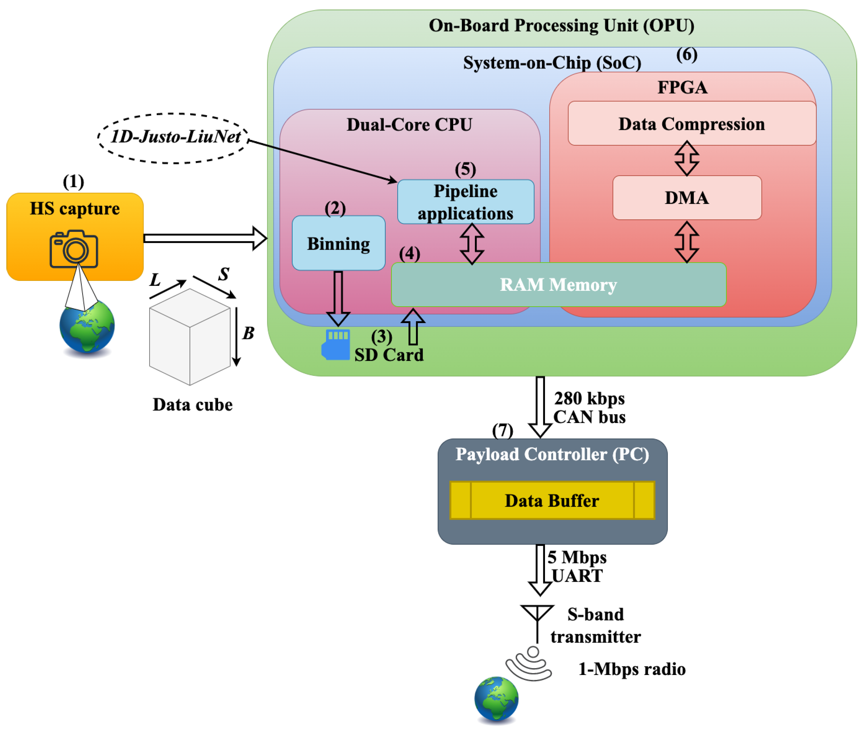
Figure 1.
HYPSO-1 system architecture general pipeline.
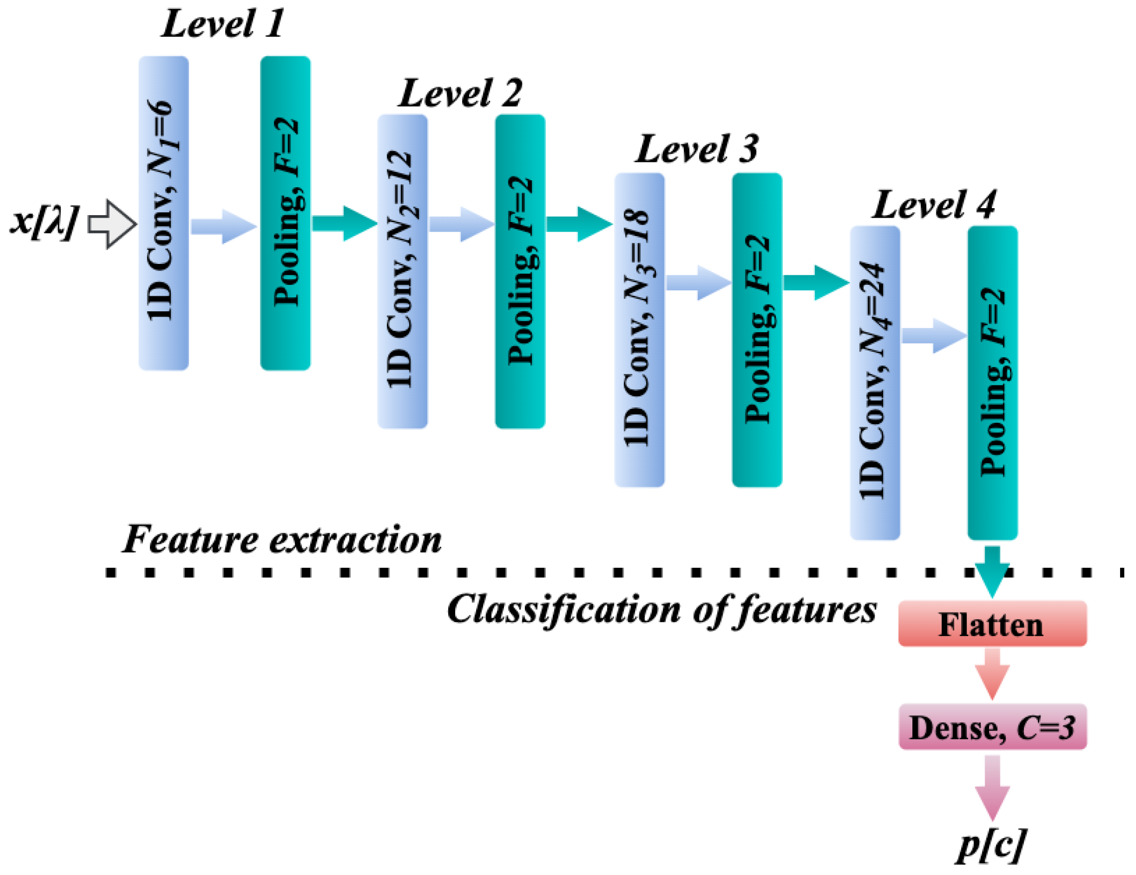
Figure 2.
Architecture of
1D-Justo-LiuNet for feature extraction and classification proposed in our previous work in [
39].
Figure 2.
Architecture of
1D-Justo-LiuNet for feature extraction and classification proposed in our previous work in [
39].
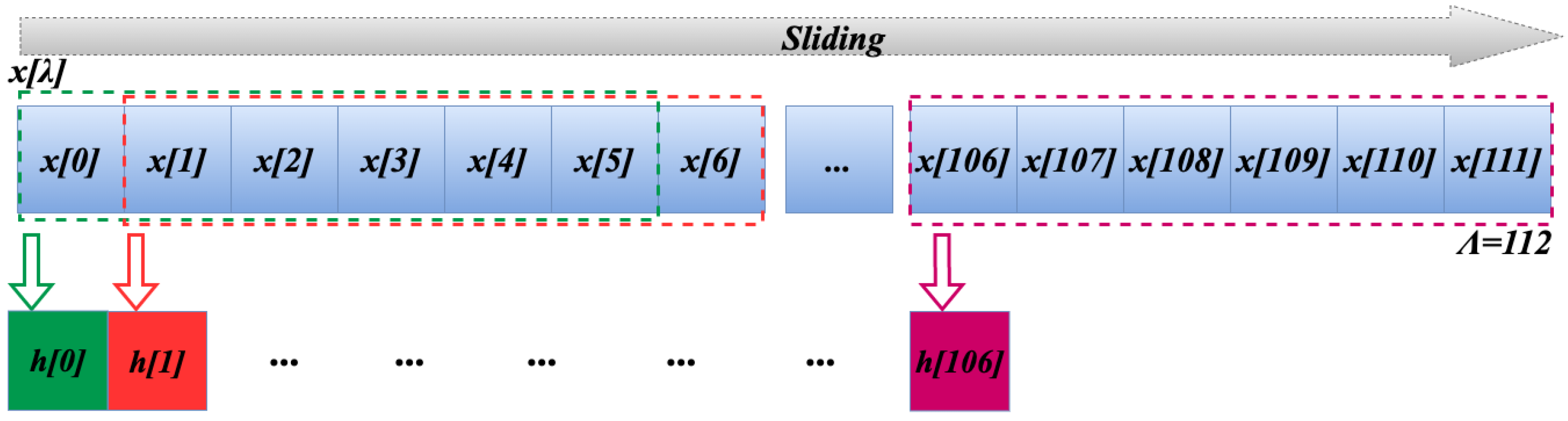
Figure 3.
Sliding process with stride over .
Figure 3.
Sliding process with stride over .
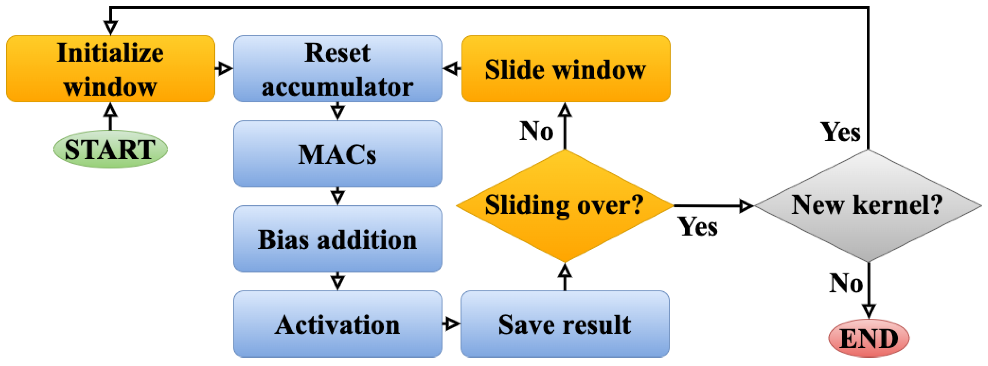
Figure 4.
Flow diagram of operations in the convolution layer (Implementation 1).
Figure 4.
Flow diagram of operations in the convolution layer (Implementation 1).
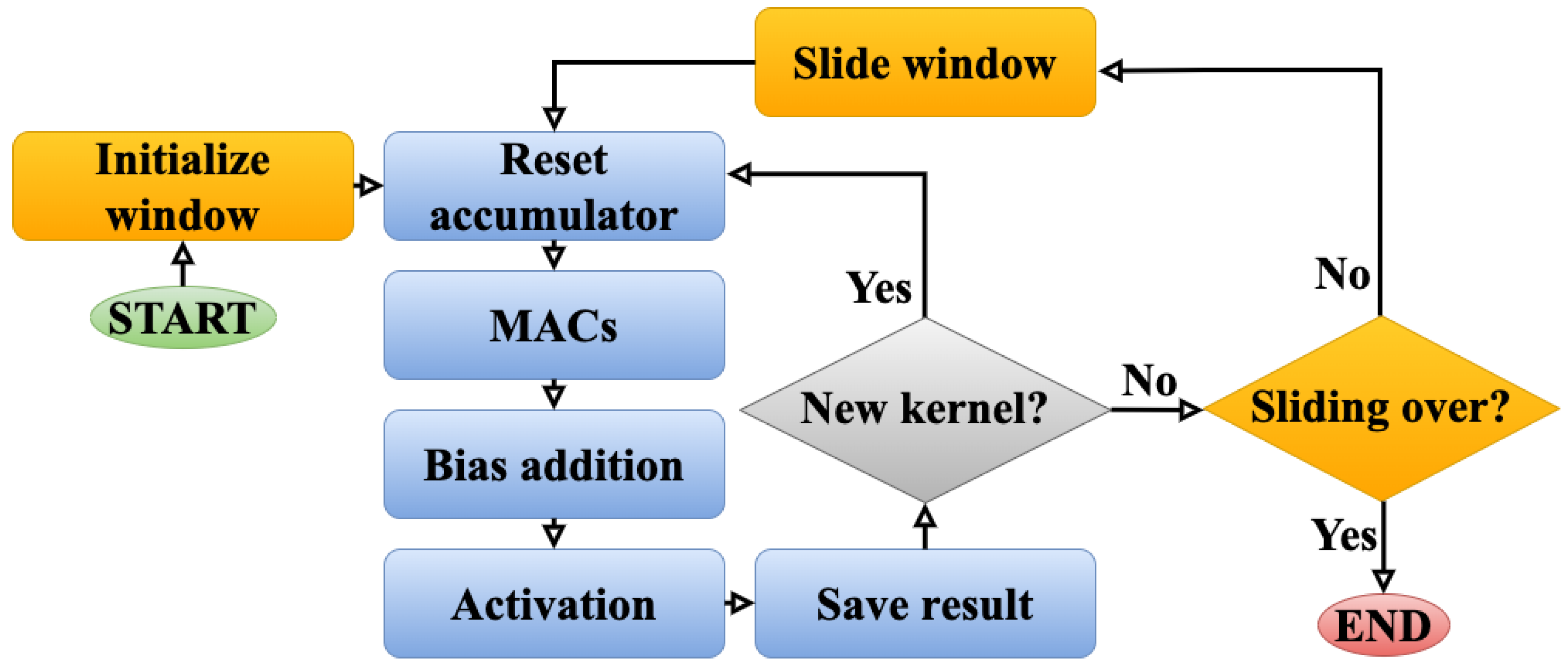
Figure 5.
Flow diagram of operations in the convolution layer (Implementation 2).
Figure 5.
Flow diagram of operations in the convolution layer (Implementation 2).
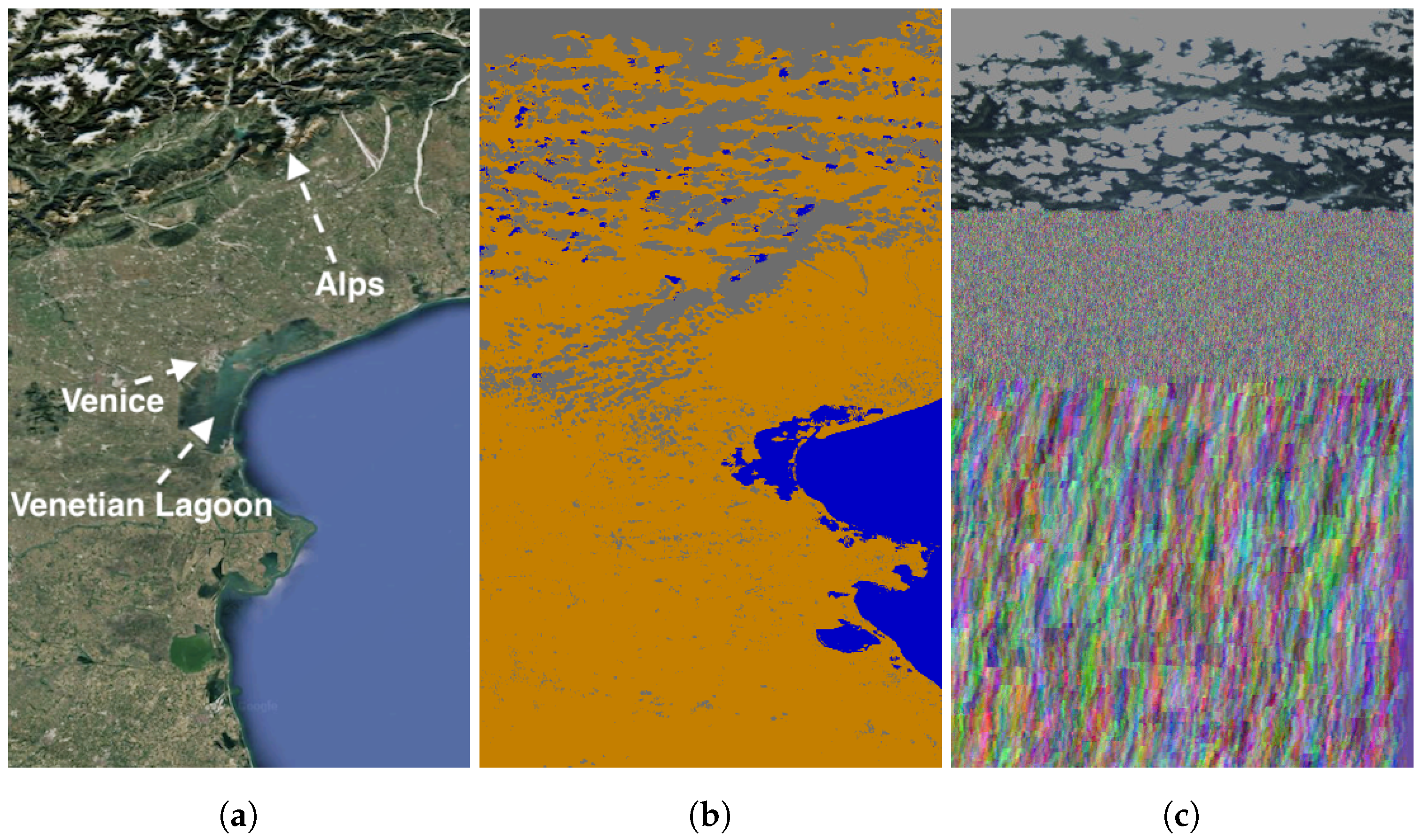
Figure 6.
Venice, Italy, Europe, on 22 June 2024 at 09:44 UTC+00. Coordinates: 45.3° latitude and 12.5° longitude. Solar zenith angle: 28.7°; exposure time: 35 ms. (a) Planned geographical area. (b) Segmented image in orbit. (c) RGB composite from cube.
Figure 6.
Venice, Italy, Europe, on 22 June 2024 at 09:44 UTC+00. Coordinates: 45.3° latitude and 12.5° longitude. Solar zenith angle: 28.7°; exposure time: 35 ms. (a) Planned geographical area. (b) Segmented image in orbit. (c) RGB composite from cube.
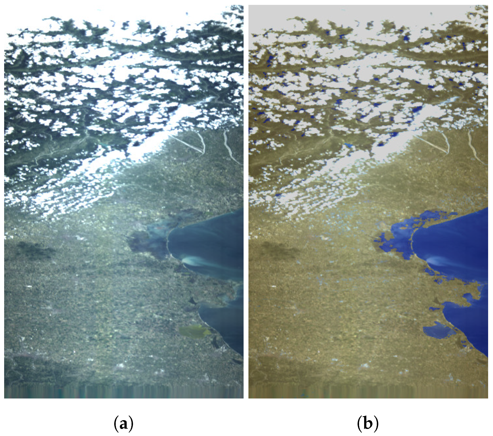
Figure 7.
Venice, Italy, Europe, on 22 June 2024 at 09:44 UTC-retransmitted. (a) RGB composite from cube. (b) Segmented image overlaid.
Figure 7.
Venice, Italy, Europe, on 22 June 2024 at 09:44 UTC-retransmitted. (a) RGB composite from cube. (b) Segmented image overlaid.
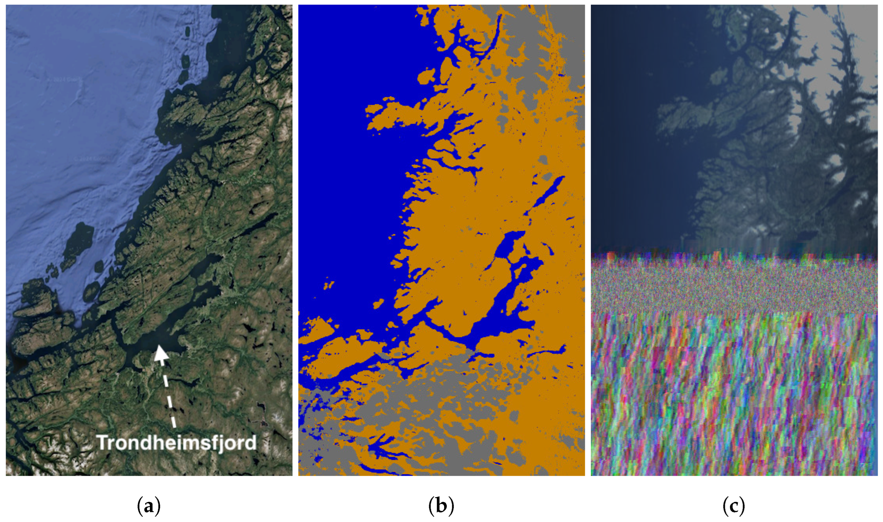
Figure 8.
Trondheim, Norway, Europe, on 17 May 2024 at 10:54 UTC. Coordinates: 63.6° latitude and 9.84° longitude. Solar zenith angle: 44.9°; exposure time: 50 ms. (a) Planned geographical area. (b) Segmented image in orbit. (c) RGB composite from cube.
Figure 8.
Trondheim, Norway, Europe, on 17 May 2024 at 10:54 UTC. Coordinates: 63.6° latitude and 9.84° longitude. Solar zenith angle: 44.9°; exposure time: 50 ms. (a) Planned geographical area. (b) Segmented image in orbit. (c) RGB composite from cube.
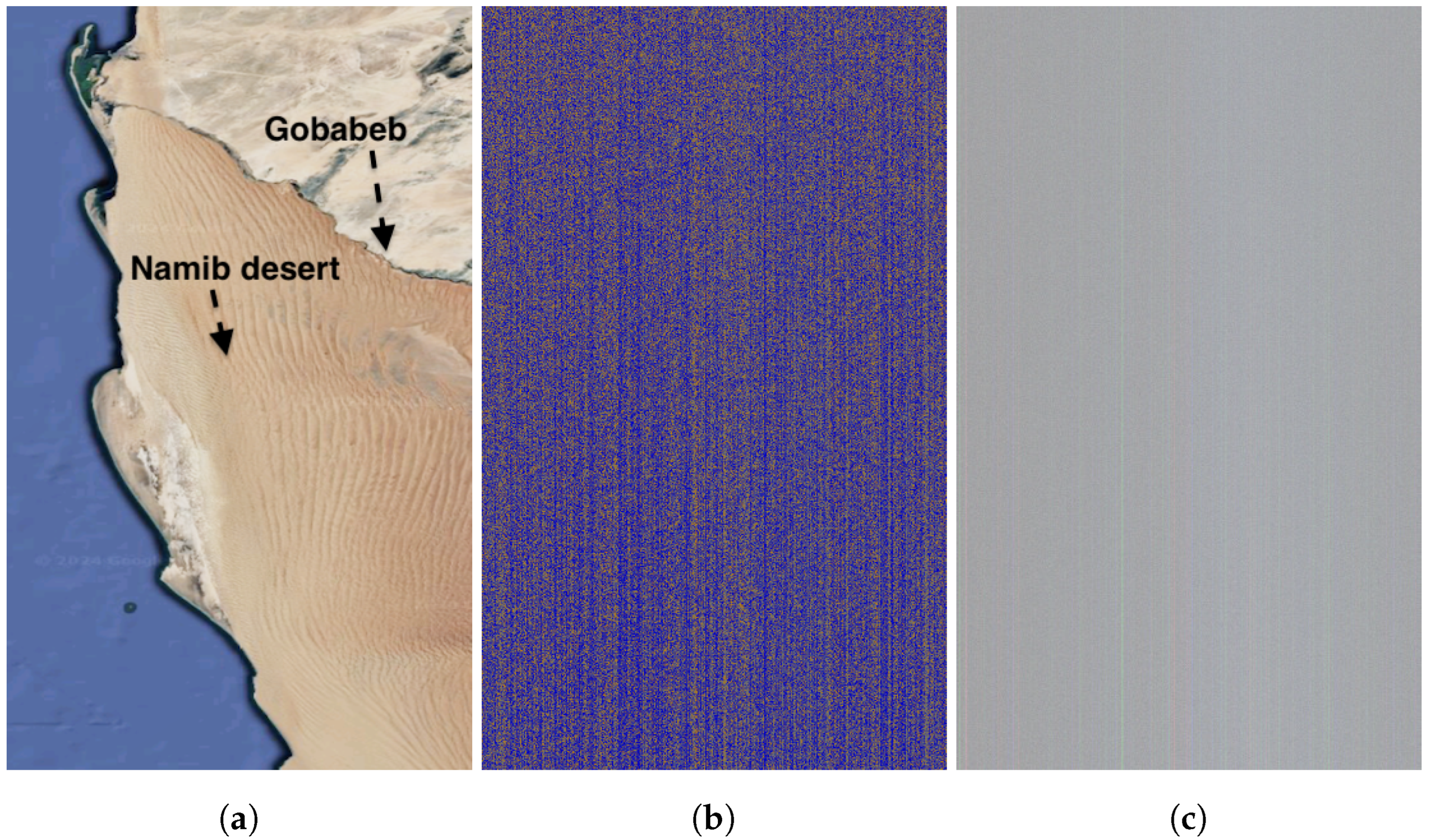
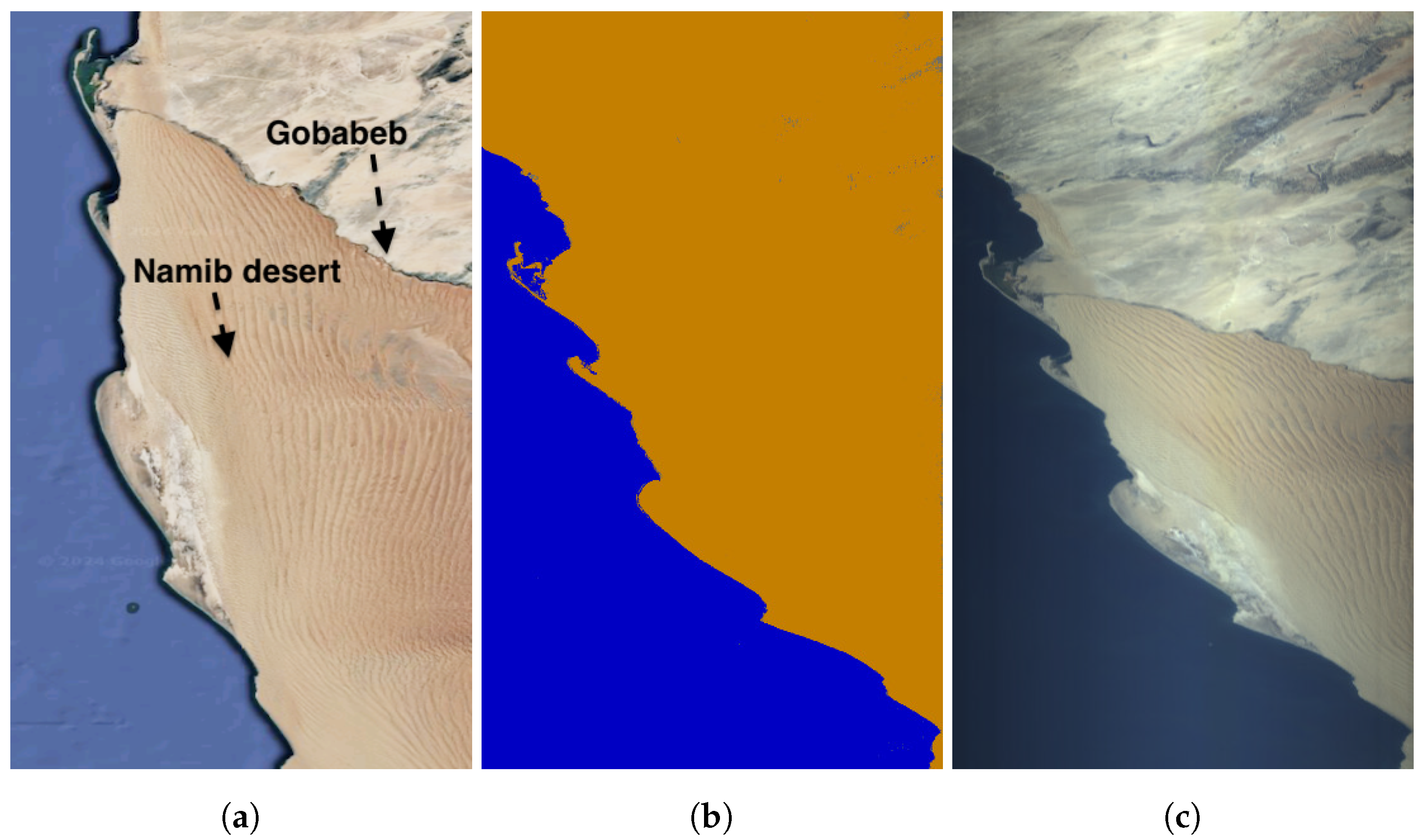
Figure 9.
Namib desert close to Gobabeb, Namibia, Africa, on 25 June 2024 at 08:51 UTC. Coordinates: −23.6° latitude and 15.0° longitude. Exposure time: 20 ms. (a) Planned geographical area. (b) Segmented image in orbit. (c) RGB composite from cube.
Figure 9.
Namib desert close to Gobabeb, Namibia, Africa, on 25 June 2024 at 08:51 UTC. Coordinates: −23.6° latitude and 15.0° longitude. Exposure time: 20 ms. (a) Planned geographical area. (b) Segmented image in orbit. (c) RGB composite from cube.
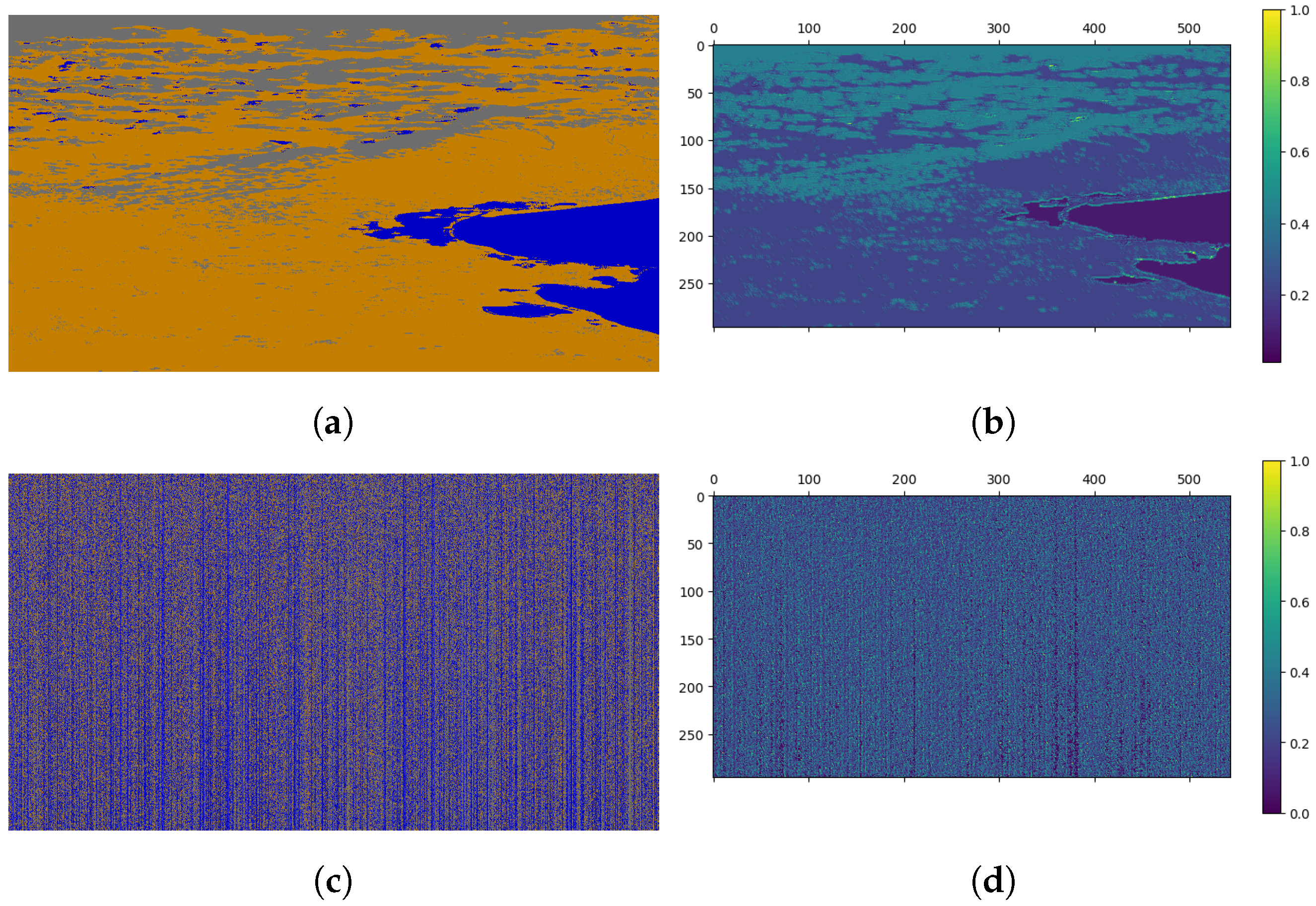
Figure 10.
Grad-CAM explanations for classification of segmented images. (a) Segmented image (no mispointing). (b) Grad-CAM explanation. (c) Segmented image (mispointing). (d) Grad-CAM explanation.
Figure 10.
Grad-CAM explanations for classification of segmented images. (a) Segmented image (no mispointing). (b) Grad-CAM explanation. (c) Segmented image (mispointing). (d) Grad-CAM explanation.
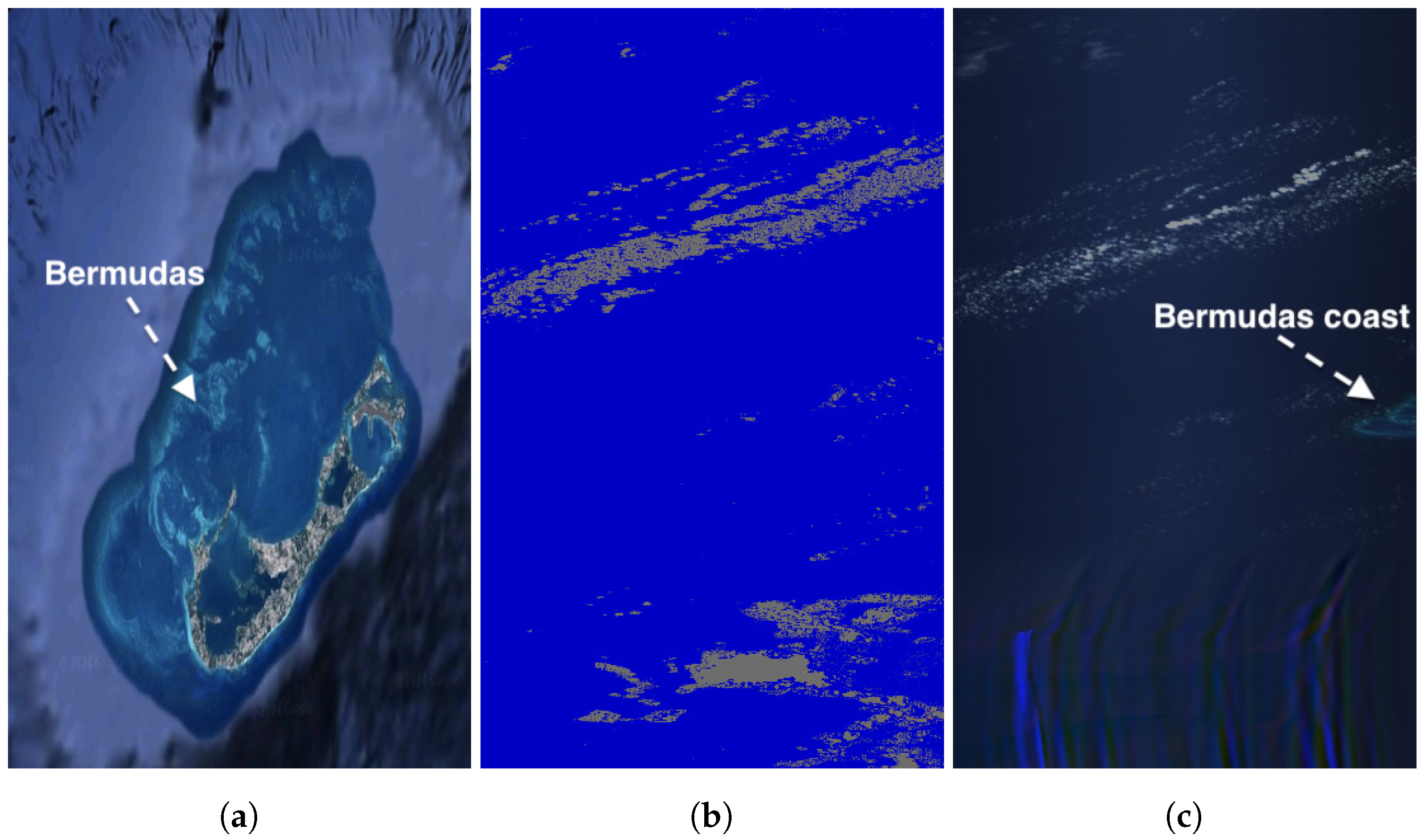
Figure 11.
Bermuda Archipelago, British Overseas, Atlantic Ocean, on 16 July 2024 at 14:27 UTC. Coordinates: 32.4° latitude and −64.8° longitude. Solar zenith angle: 32.6°; exposure time: 30 ms. (a) Planned geographical area. (b) Segmented image in orbit. (c) RGB composite from cube.
Figure 11.
Bermuda Archipelago, British Overseas, Atlantic Ocean, on 16 July 2024 at 14:27 UTC. Coordinates: 32.4° latitude and −64.8° longitude. Solar zenith angle: 32.6°; exposure time: 30 ms. (a) Planned geographical area. (b) Segmented image in orbit. (c) RGB composite from cube.
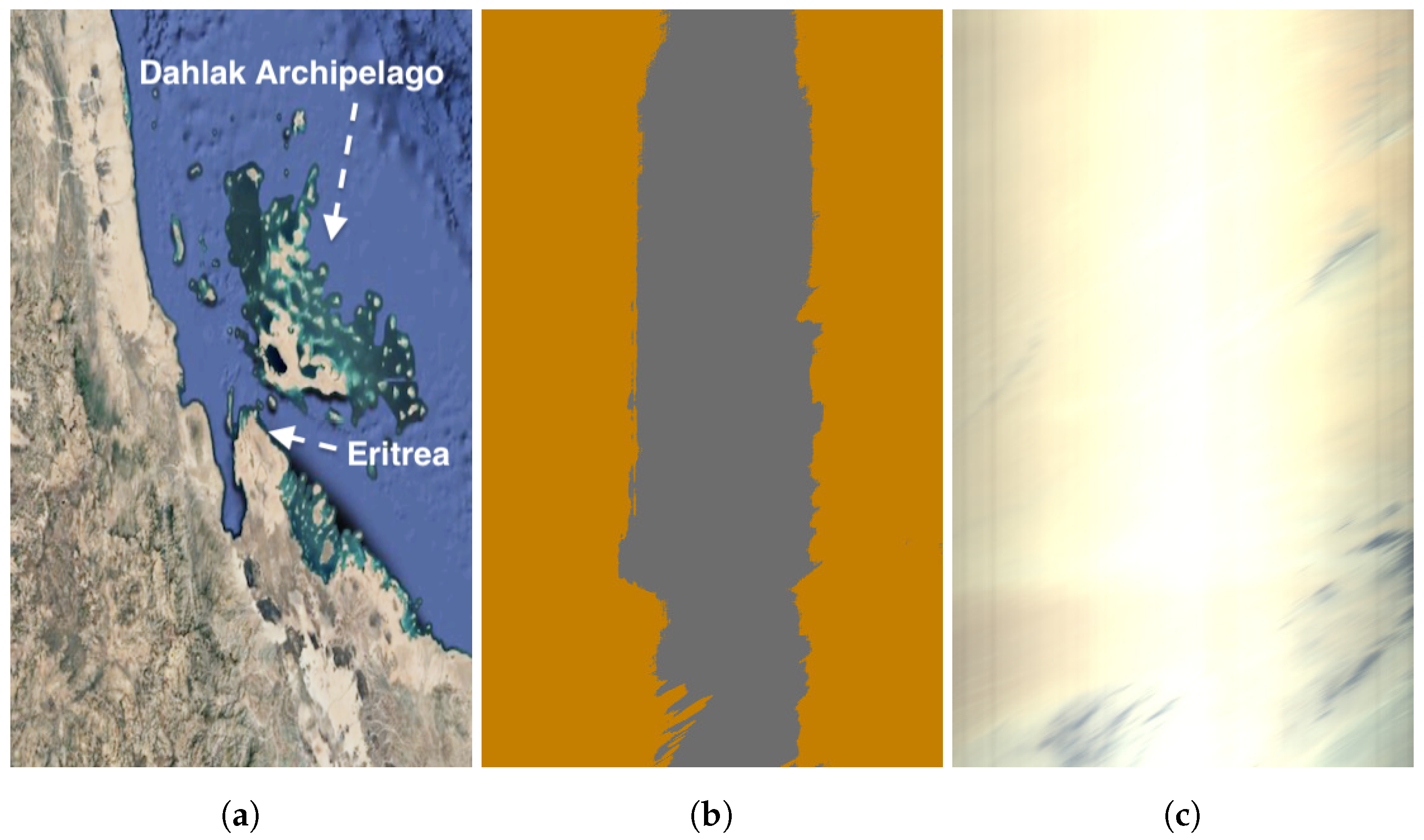
Figure 12.
Dahlak Archipelago, Eritrea, Africa, on 16 June 2024 at 07:28 UTC. Coordinates: 16.0° latitude and 40.4° longitude. Solar zenith angle: 16.0°; exposure time: 25 ms. (a) Planned geographical area. (b) Segmented image in orbit. (c) RGB composite from cube.
Figure 12.
Dahlak Archipelago, Eritrea, Africa, on 16 June 2024 at 07:28 UTC. Coordinates: 16.0° latitude and 40.4° longitude. Solar zenith angle: 16.0°; exposure time: 25 ms. (a) Planned geographical area. (b) Segmented image in orbit. (c) RGB composite from cube.
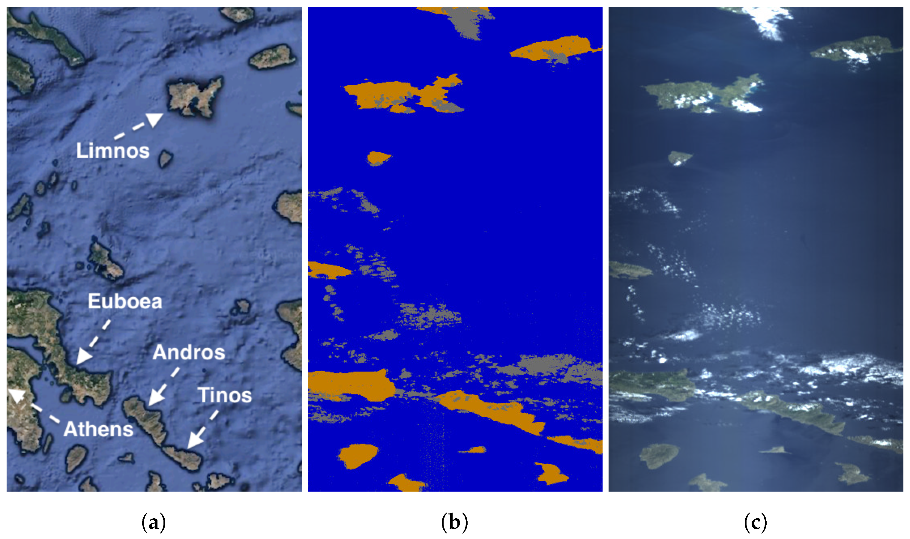
Figure 13.
Aegean Archipelago, Greece, Europe, on 2 May 2024 at 08:44 UTC. Coordinates: 38.5° latitude and 25.2° longitude. Solar zenith angle: 39.0°; exposure time: 30 ms. (a) Planned geographical area. (b) Segmented image in orbit. (c) RGB composite from cube.
Figure 13.
Aegean Archipelago, Greece, Europe, on 2 May 2024 at 08:44 UTC. Coordinates: 38.5° latitude and 25.2° longitude. Solar zenith angle: 39.0°; exposure time: 30 ms. (a) Planned geographical area. (b) Segmented image in orbit. (c) RGB composite from cube.
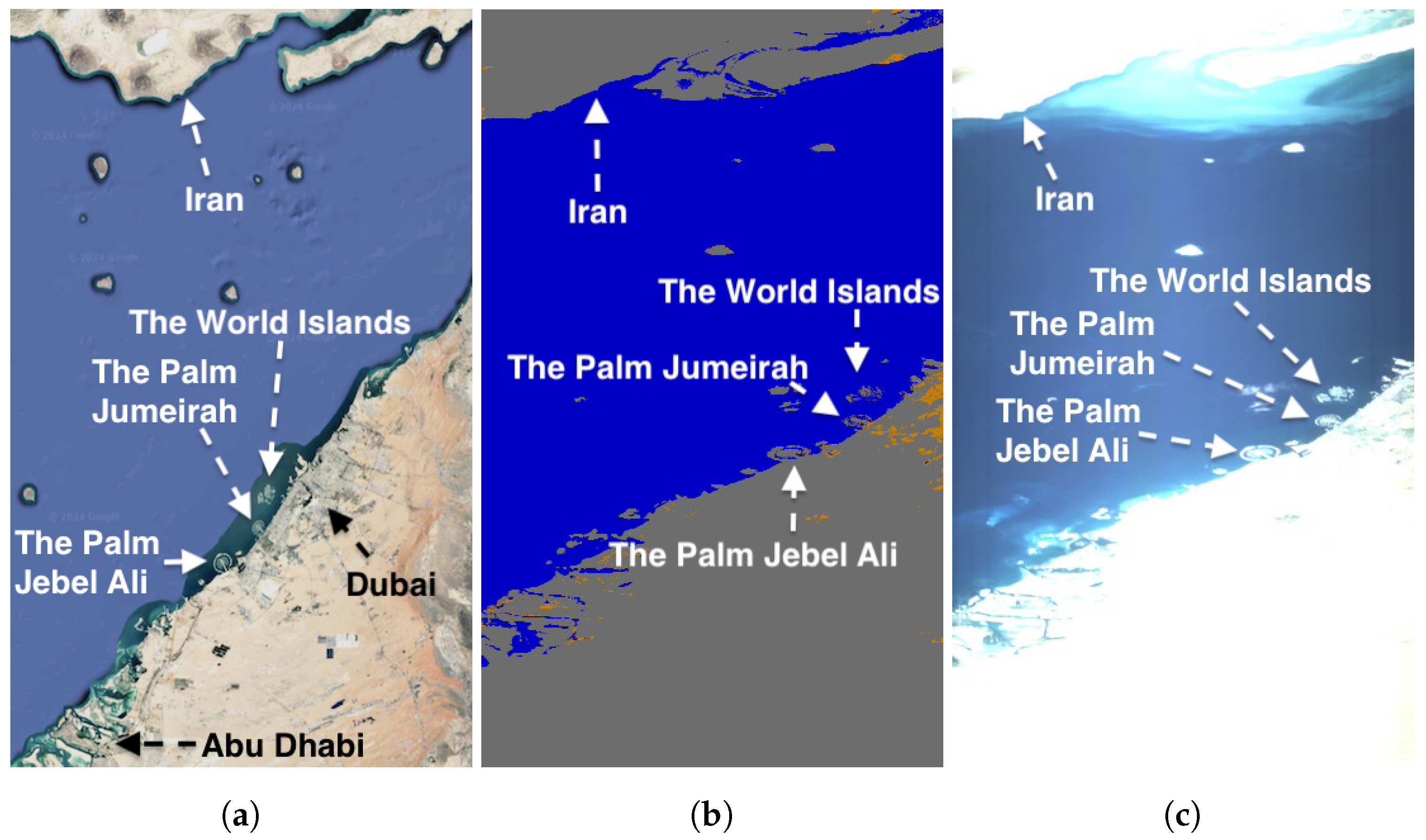
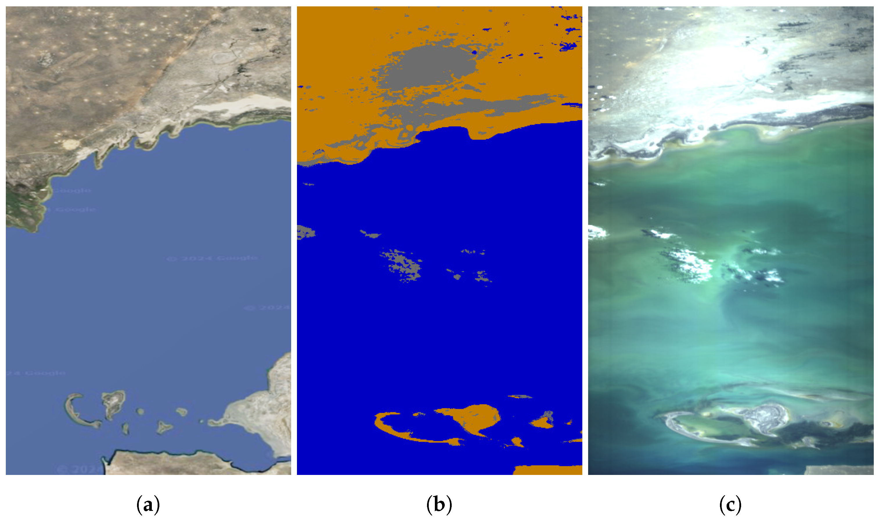
Figure 14.
Abu Dhabi and Dubai, United Arab Emirates, Asia, on 9 May 2024 at 06:12 UTC. Coordinates: 25.3° latitude and 54.7° longitude. Solar zenith angle: 29.5°; exposure time: 40 ms. (a) Planned geographical area. (b) Segmented image in orbit. (c) RGB composite from cube.
Figure 14.
Abu Dhabi and Dubai, United Arab Emirates, Asia, on 9 May 2024 at 06:12 UTC. Coordinates: 25.3° latitude and 54.7° longitude. Solar zenith angle: 29.5°; exposure time: 40 ms. (a) Planned geographical area. (b) Segmented image in orbit. (c) RGB composite from cube.
Figure 15.
Abu Dhabi and Dubai, United Arab Emirates, Asia, on 27 June 2024 at 06:17 UTC. Coordinates: 25.1° latitude and 55.0° longitude. Solar zenith angle: 28.9°; exposure time: 40 ms. (a) Segmented image in orbit. (b) RGB composite from cube.
Figure 15.
Abu Dhabi and Dubai, United Arab Emirates, Asia, on 27 June 2024 at 06:17 UTC. Coordinates: 25.1° latitude and 55.0° longitude. Solar zenith angle: 28.9°; exposure time: 40 ms. (a) Segmented image in orbit. (b) RGB composite from cube.
Figure 16.
Namib desert close to Gobabeb, Namibia, Africa, on 13 June 2024 at 08:49 UTC. Coordinates: −23.6° latitude and 15.0° longitude. Solar zenith angle: 56.8°; exposure time: 20 ms. (a) Planned geographical area. (b) Segmented image in orbit. (c) RGB composite from cube.
Figure 16.
Namib desert close to Gobabeb, Namibia, Africa, on 13 June 2024 at 08:49 UTC. Coordinates: −23.6° latitude and 15.0° longitude. Solar zenith angle: 56.8°; exposure time: 20 ms. (a) Planned geographical area. (b) Segmented image in orbit. (c) RGB composite from cube.
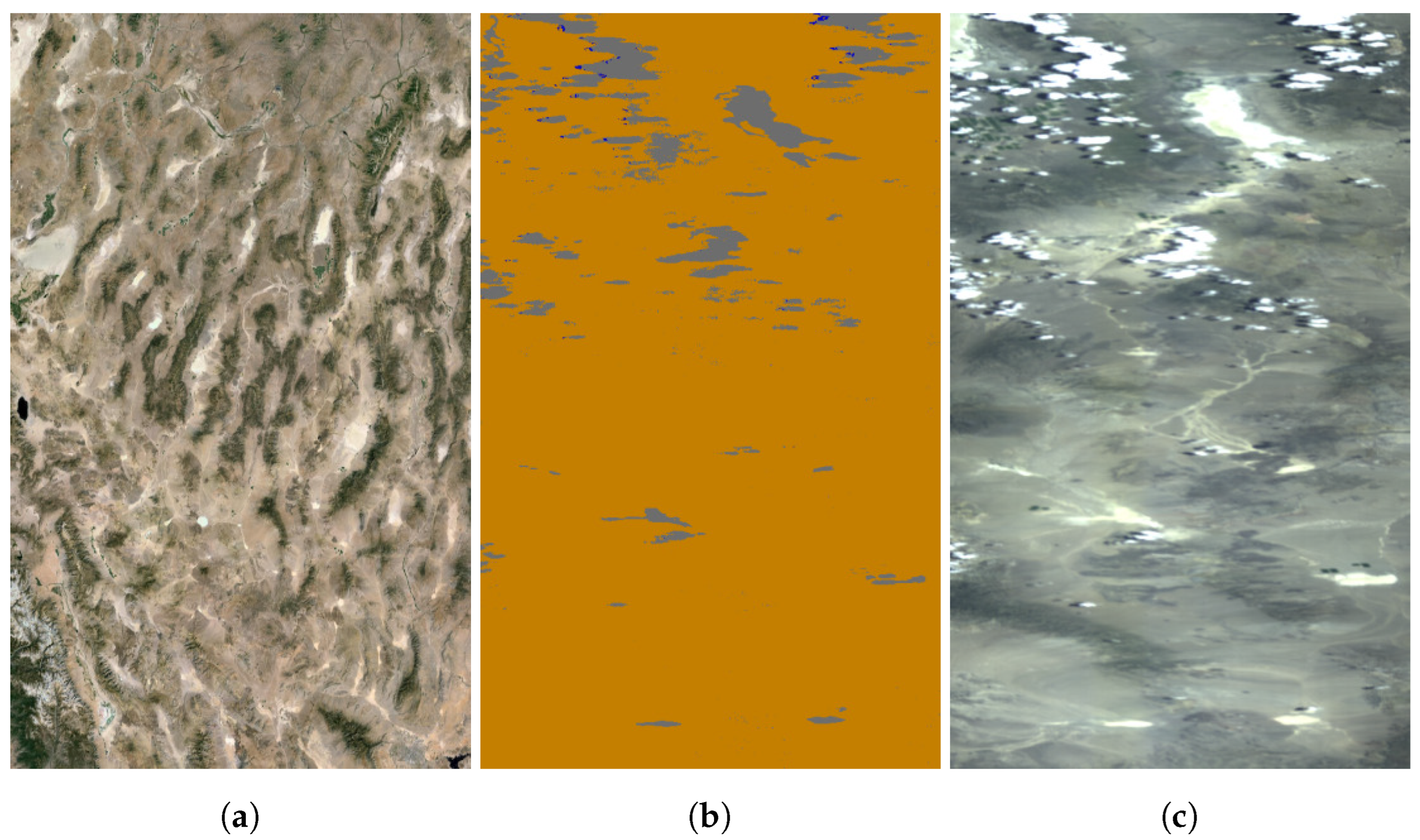
Figure 17.
Mojave Desert, USA, North America, on 28 May 2024 at 17:52 UTC. Coordinates: 38.7° latitude and −116.1° longitude. Solar zenith angle: 28.9°; exposure time: 20 ms. (a) Planned geographical area. (b) Segmented image in orbit. (c) RGB composite from cube.
Figure 17.
Mojave Desert, USA, North America, on 28 May 2024 at 17:52 UTC. Coordinates: 38.7° latitude and −116.1° longitude. Solar zenith angle: 28.9°; exposure time: 20 ms. (a) Planned geographical area. (b) Segmented image in orbit. (c) RGB composite from cube.
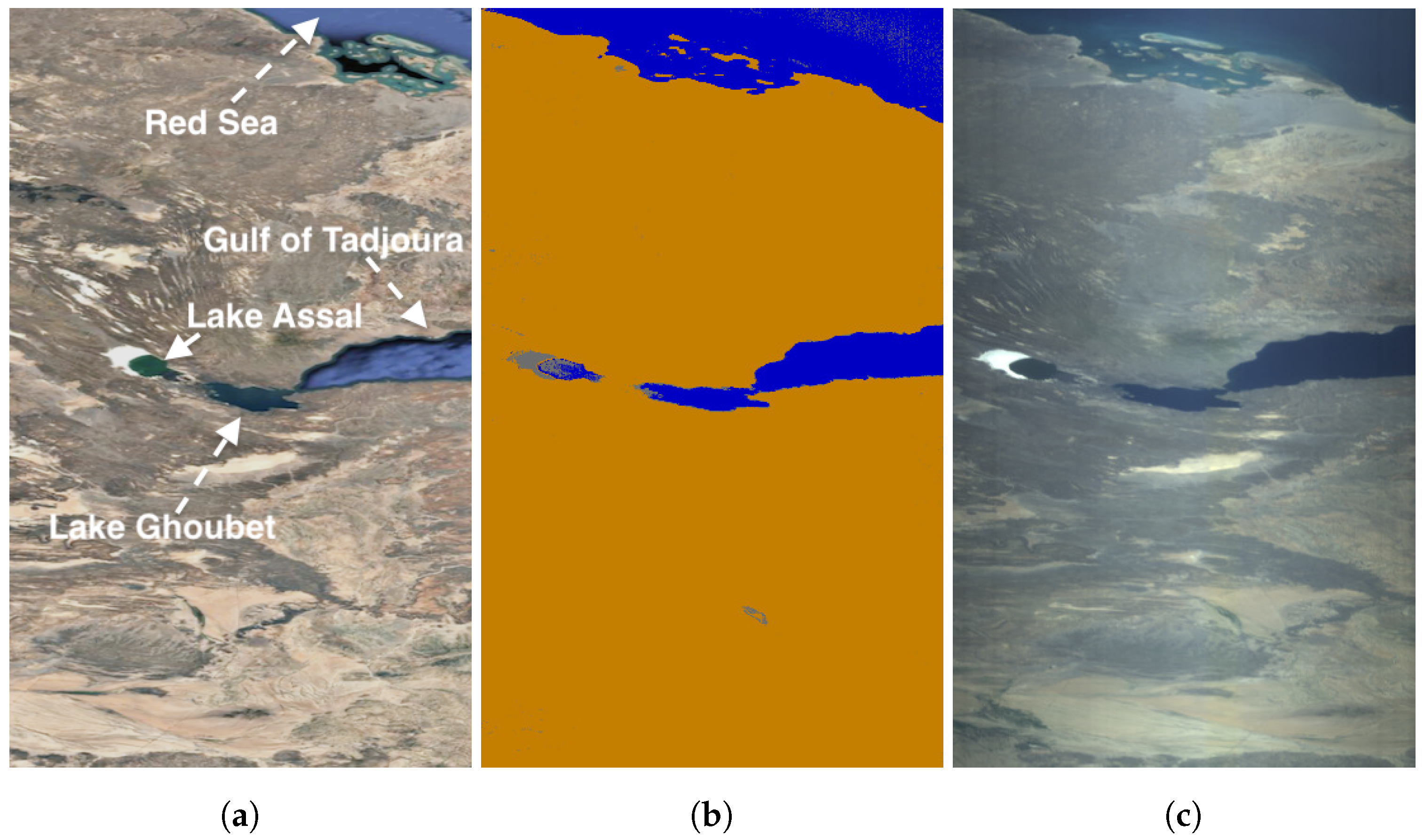
Figure 18.
Lake Assal near Gulf of Tadjoura and the Red Sea, Djibouti, Africa, on 28 May 2024 at 06:57 UTC. Coordinates: 11.6° latitude and 42.8° longitude. Solar zenith angle: 32.6°; exposure time: 20 ms. (a) Planned geographical area. (b) Segmented image in orbit. (c) RGB composite from cube.
Figure 18.
Lake Assal near Gulf of Tadjoura and the Red Sea, Djibouti, Africa, on 28 May 2024 at 06:57 UTC. Coordinates: 11.6° latitude and 42.8° longitude. Solar zenith angle: 32.6°; exposure time: 20 ms. (a) Planned geographical area. (b) Segmented image in orbit. (c) RGB composite from cube.
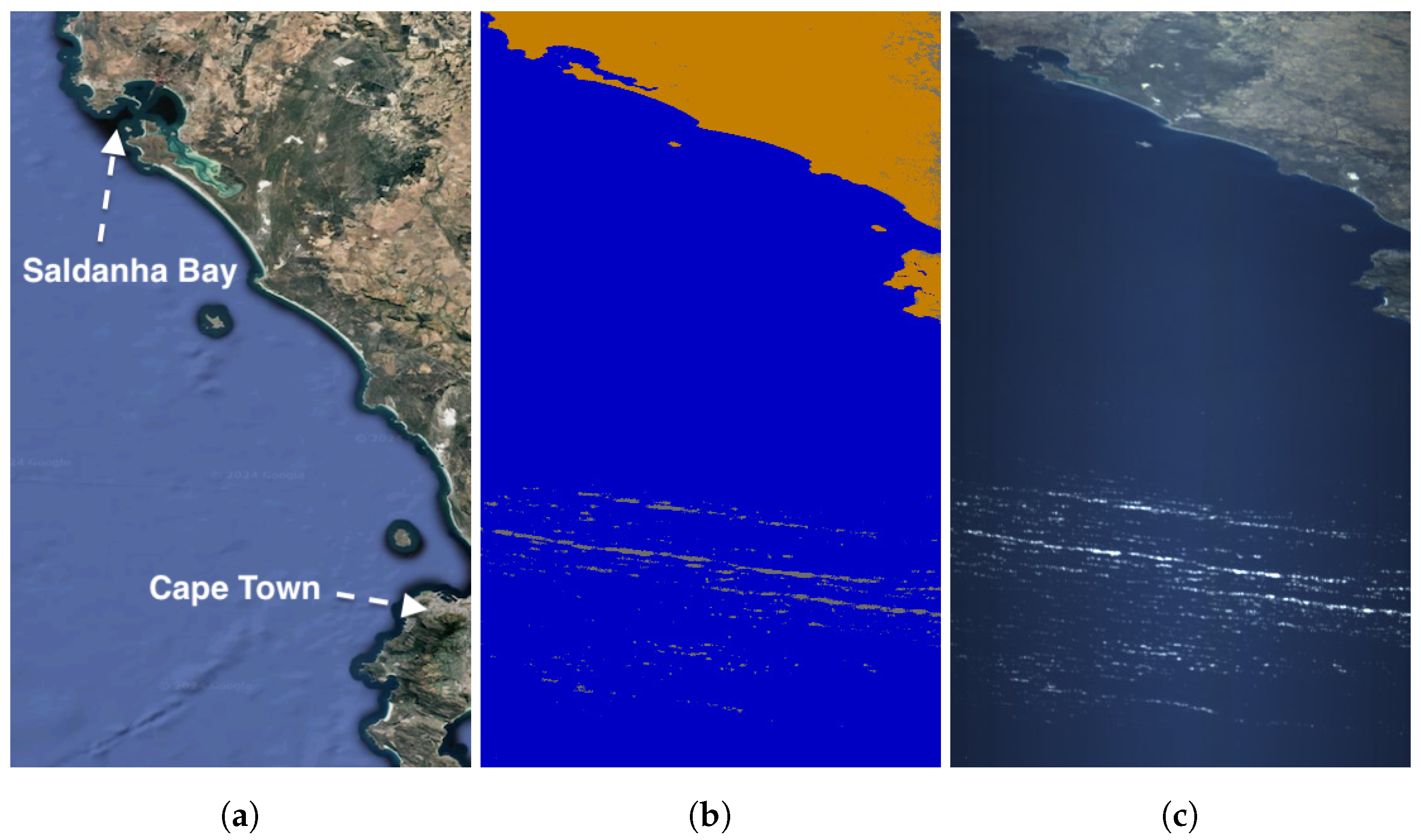
Figure 19.
Cape Town, South Africa, Africa, on 13 April 2024 at 08:06 UTC. Coordinates: −34.3° latitude and 18.2° longitude. Solar zenith angle: 58.1°; exposure time: 30 ms. (a) Planned geographical area. (b) Segmented image in orbit. (c) RGB composite from cube.
Figure 19.
Cape Town, South Africa, Africa, on 13 April 2024 at 08:06 UTC. Coordinates: −34.3° latitude and 18.2° longitude. Solar zenith angle: 58.1°; exposure time: 30 ms. (a) Planned geographical area. (b) Segmented image in orbit. (c) RGB composite from cube.
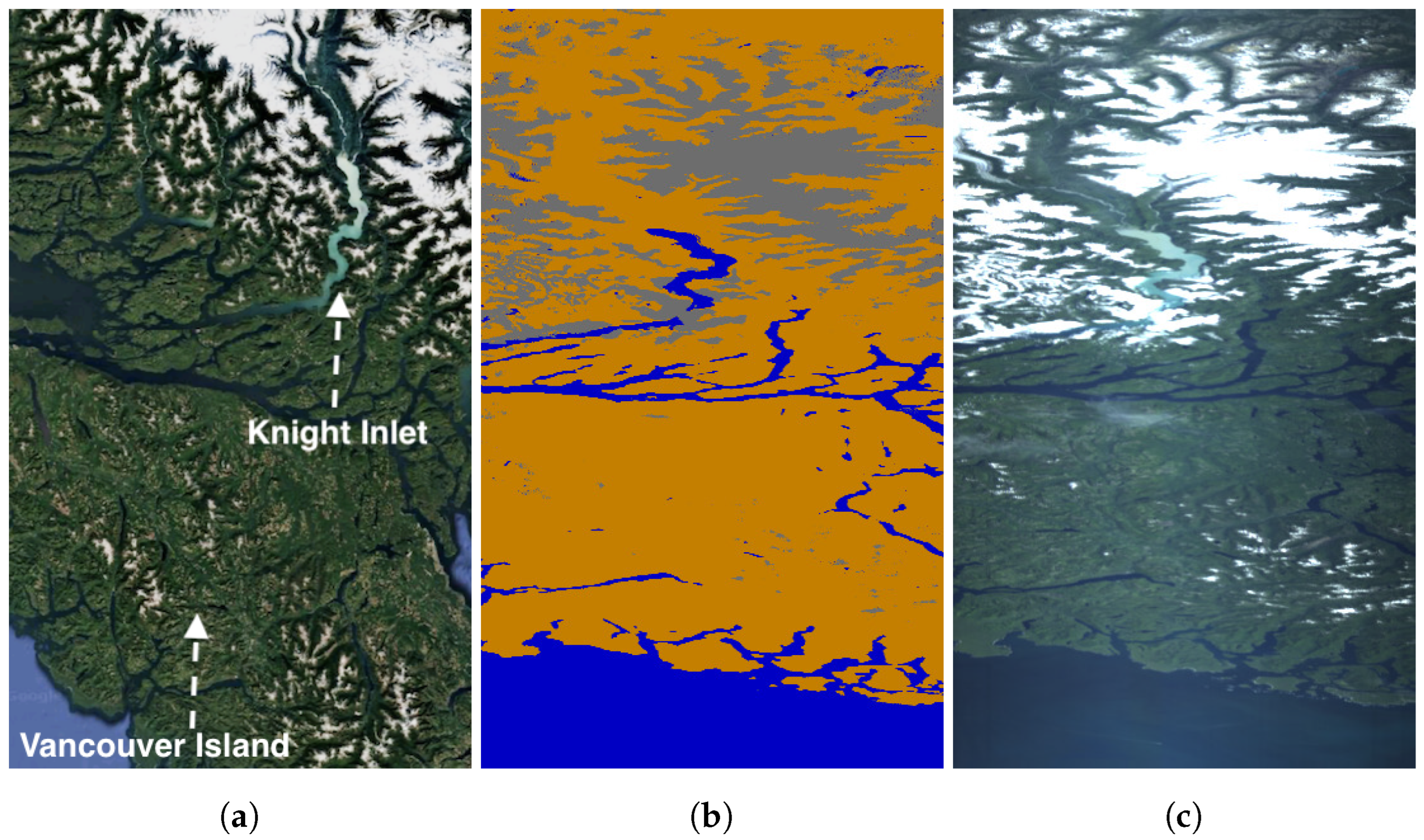
Figure 20.
Vancouver Island, Canada, North America, on 13 July 2024 at 18:43 UTC. Coordinates: 50.4° latitude and −126.0° longitude. Solar zenith angle: 35.2°; exposure time: 30 ms. (a) Planned geographical area. (b) Segmented image in orbit. (c) RGB composite from cube.
Figure 20.
Vancouver Island, Canada, North America, on 13 July 2024 at 18:43 UTC. Coordinates: 50.4° latitude and −126.0° longitude. Solar zenith angle: 35.2°; exposure time: 30 ms. (a) Planned geographical area. (b) Segmented image in orbit. (c) RGB composite from cube.
Figure 21.
Caspian Sea, Asia, on 7 July 2024 at 06:58 UTC. Coordinates: 46.2° latitude and 50.4° longitude. Solar zenith angle: 31.4°; exposure time: 30 ms. (a) Planned geographical area. (b) image in orbit. (c) RGB composite from cube.
Figure 21.
Caspian Sea, Asia, on 7 July 2024 at 06:58 UTC. Coordinates: 46.2° latitude and 50.4° longitude. Solar zenith angle: 31.4°; exposure time: 30 ms. (a) Planned geographical area. (b) image in orbit. (c) RGB composite from cube.
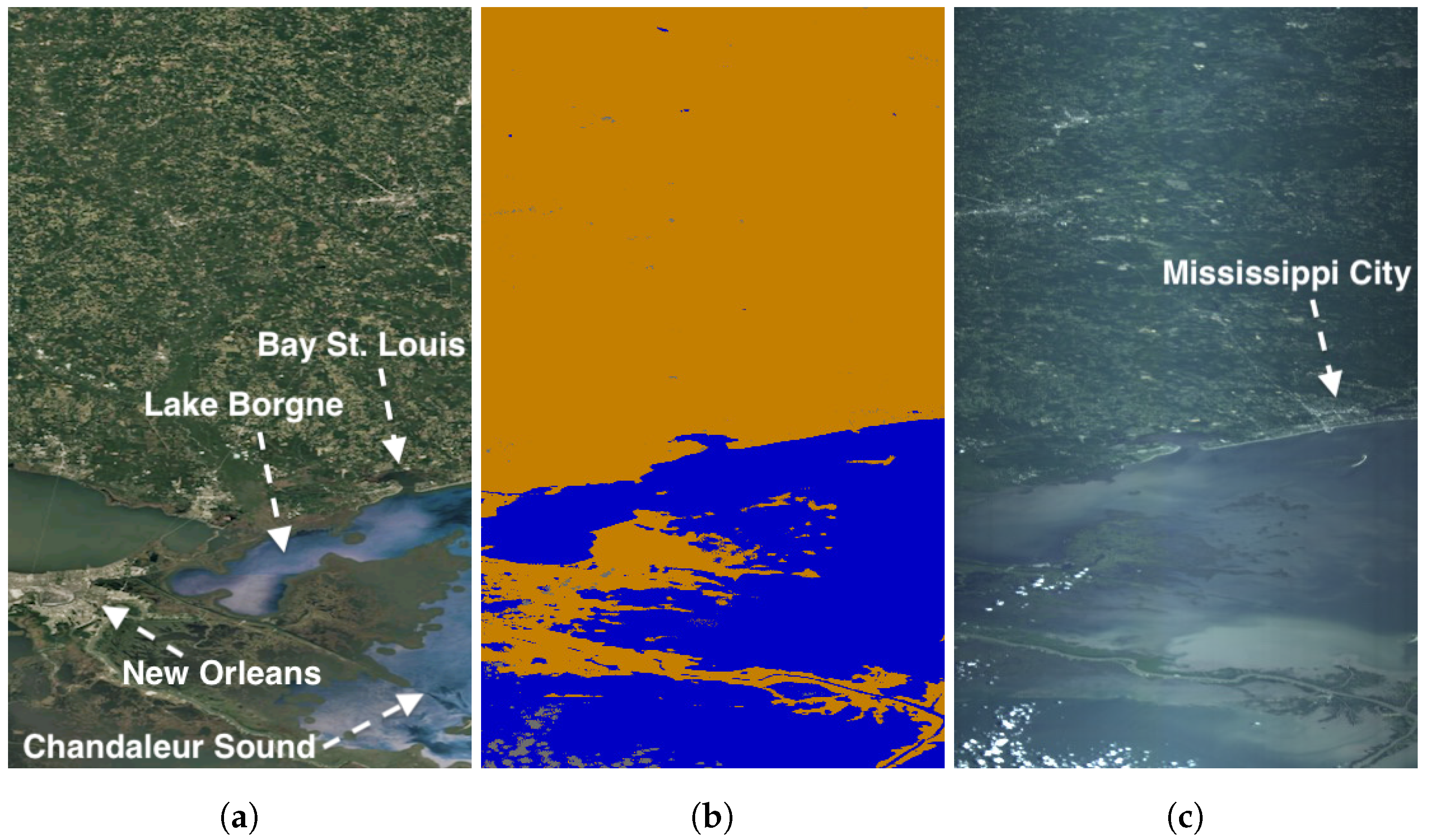
Figure 22.
New Orleans (Gulf of Mexico), USA, North America, on 14 June 2024 at 16:04 UTC. Coordinates: 30.6° latitude and −89.4° longitude. Solar zenith angle: 25.8°; exposure time: 30 ms. (a) Planned geographical area. (b) Segmented image in orbit. (c) RGB composite from cube.
Figure 22.
New Orleans (Gulf of Mexico), USA, North America, on 14 June 2024 at 16:04 UTC. Coordinates: 30.6° latitude and −89.4° longitude. Solar zenith angle: 25.8°; exposure time: 30 ms. (a) Planned geographical area. (b) Segmented image in orbit. (c) RGB composite from cube.
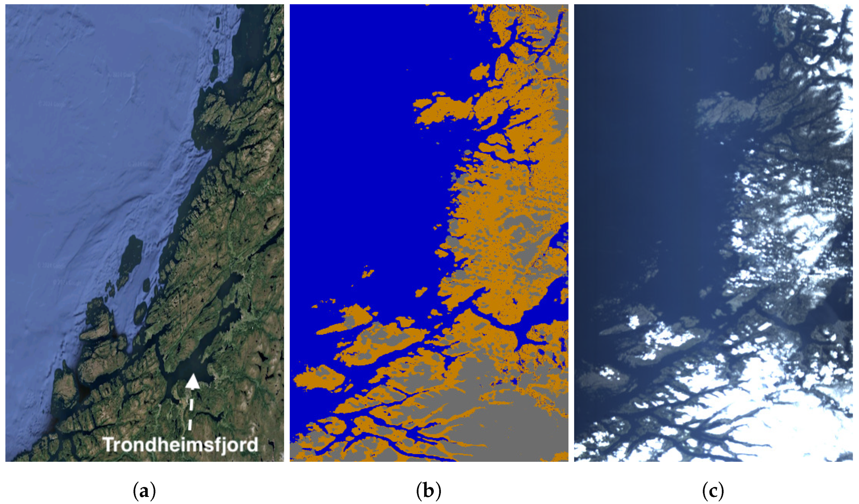
Figure 23.
Trondheim, Norway, Europe, on 26 April 2024 at 10:49 UTC. Coordinates: 64.3° latitude and 9.42° longitude. Solar zenith angle: 50.5°; exposure time: 40 ms. (a) Planned geographical area. (b) Segmented image in orbit. (c) RGB composite from cube.
Figure 23.
Trondheim, Norway, Europe, on 26 April 2024 at 10:49 UTC. Coordinates: 64.3° latitude and 9.42° longitude. Solar zenith angle: 50.5°; exposure time: 40 ms. (a) Planned geographical area. (b) Segmented image in orbit. (c) RGB composite from cube.
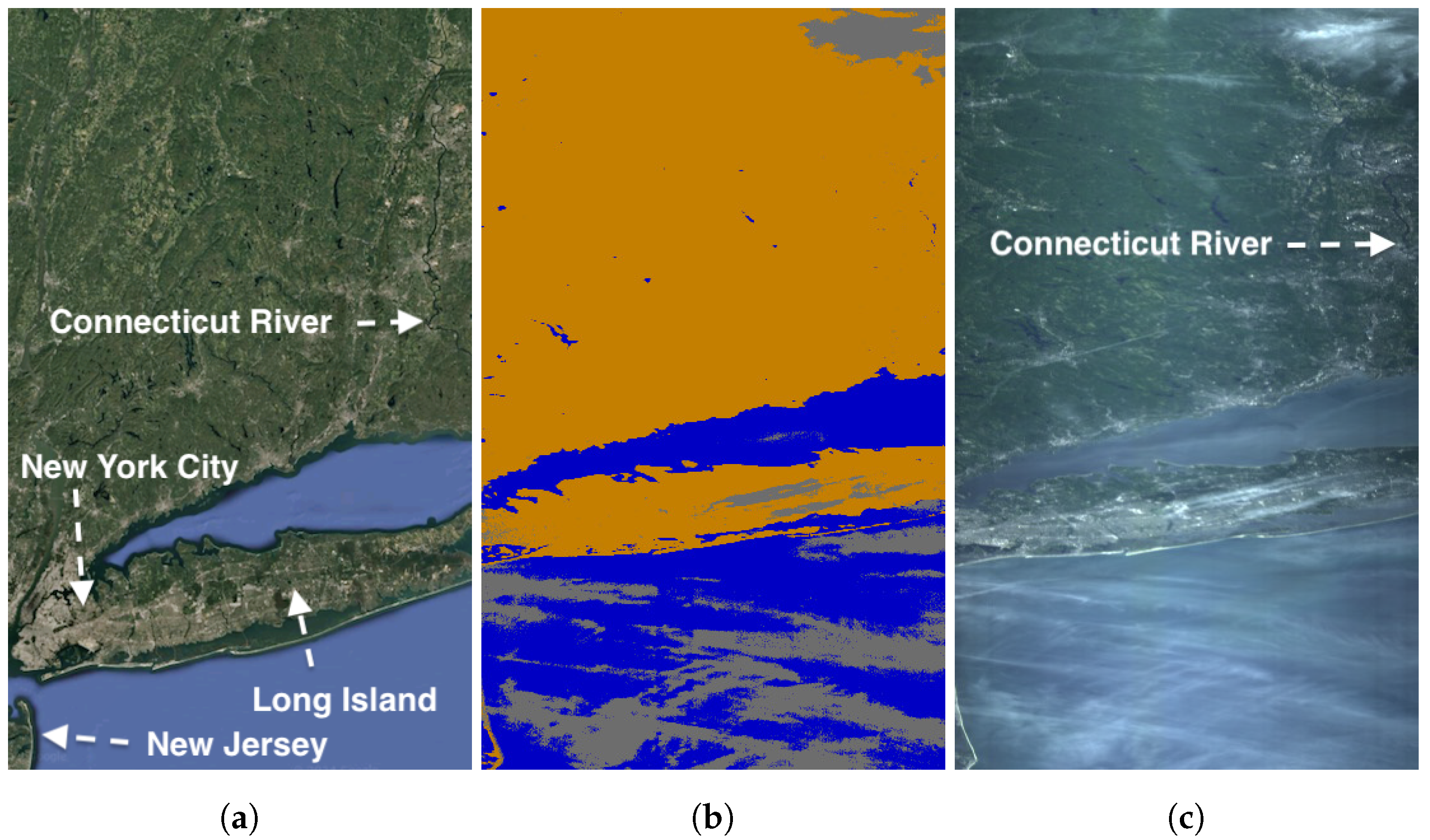
Figure 24.
Long Island - New York, USA, North America, on 16 June 2024 at 15:14 UTC. Coordinates: 41.3° latitude and −73.4° longitude. Solar zenith angle: 27.1°; exposure time: 35 ms. (a) Planned geographical area. (b) Segmented image in orbit. (c) RGB composite from cube.
Figure 24.
Long Island - New York, USA, North America, on 16 June 2024 at 15:14 UTC. Coordinates: 41.3° latitude and −73.4° longitude. Solar zenith angle: 27.1°; exposure time: 35 ms. (a) Planned geographical area. (b) Segmented image in orbit. (c) RGB composite from cube.
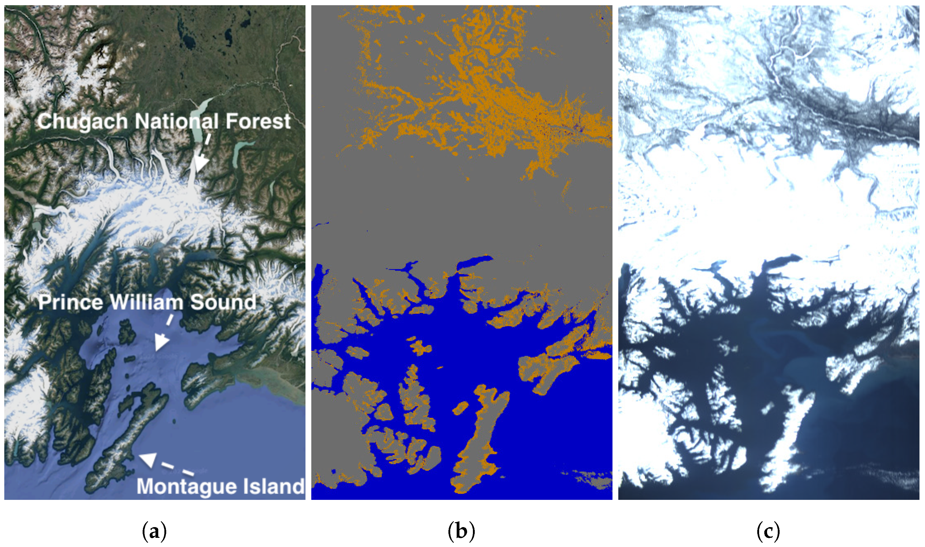
Figure 25.
Alaska, USA, North America, on 15 April 2024 at 21:08 UTC. Coordinates: 61.3° latitude and −147.1° longitude. Solar zenith angle: 51.1°; exposure time: 25 ms. (a) Planned geographical area. (b) Segmented image in orbit. (c) RGB composite from cube.
Figure 25.
Alaska, USA, North America, on 15 April 2024 at 21:08 UTC. Coordinates: 61.3° latitude and −147.1° longitude. Solar zenith angle: 51.1°; exposure time: 25 ms. (a) Planned geographical area. (b) Segmented image in orbit. (c) RGB composite from cube.
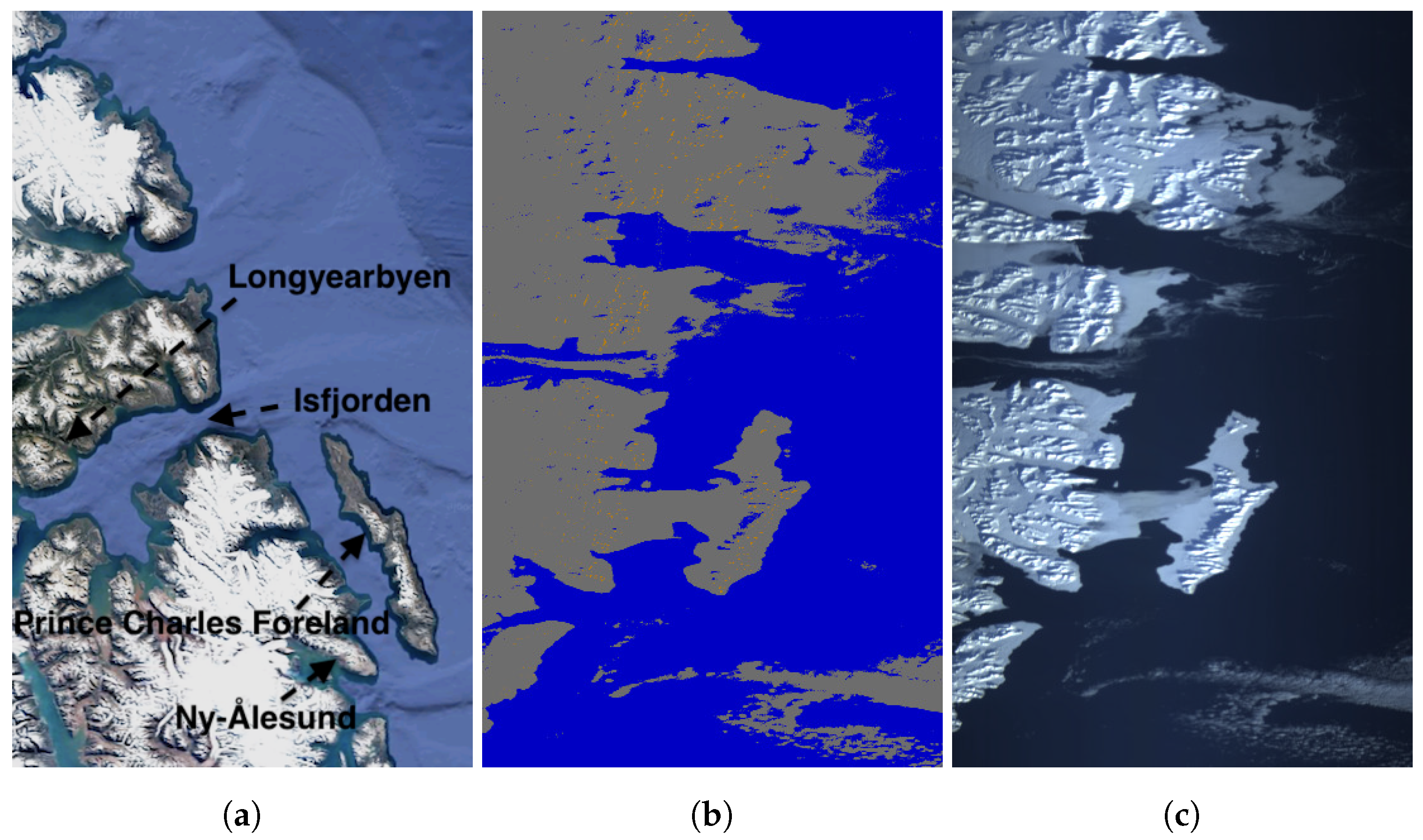
Figure 26.
Svalbard, Norway, Europe, on 3 May 2024 at 19:07 UTC. Coordinates: 78.2° latitude and 13.6° longitude. Solar zenith angle: 80.2°; exposure time: 35 ms. (a) Planned geographical area. (b) Segmented image in orbit. (c) RGB composite from cube.
Figure 26.
Svalbard, Norway, Europe, on 3 May 2024 at 19:07 UTC. Coordinates: 78.2° latitude and 13.6° longitude. Solar zenith angle: 80.2°; exposure time: 35 ms. (a) Planned geographical area. (b) Segmented image in orbit. (c) RGB composite from cube.
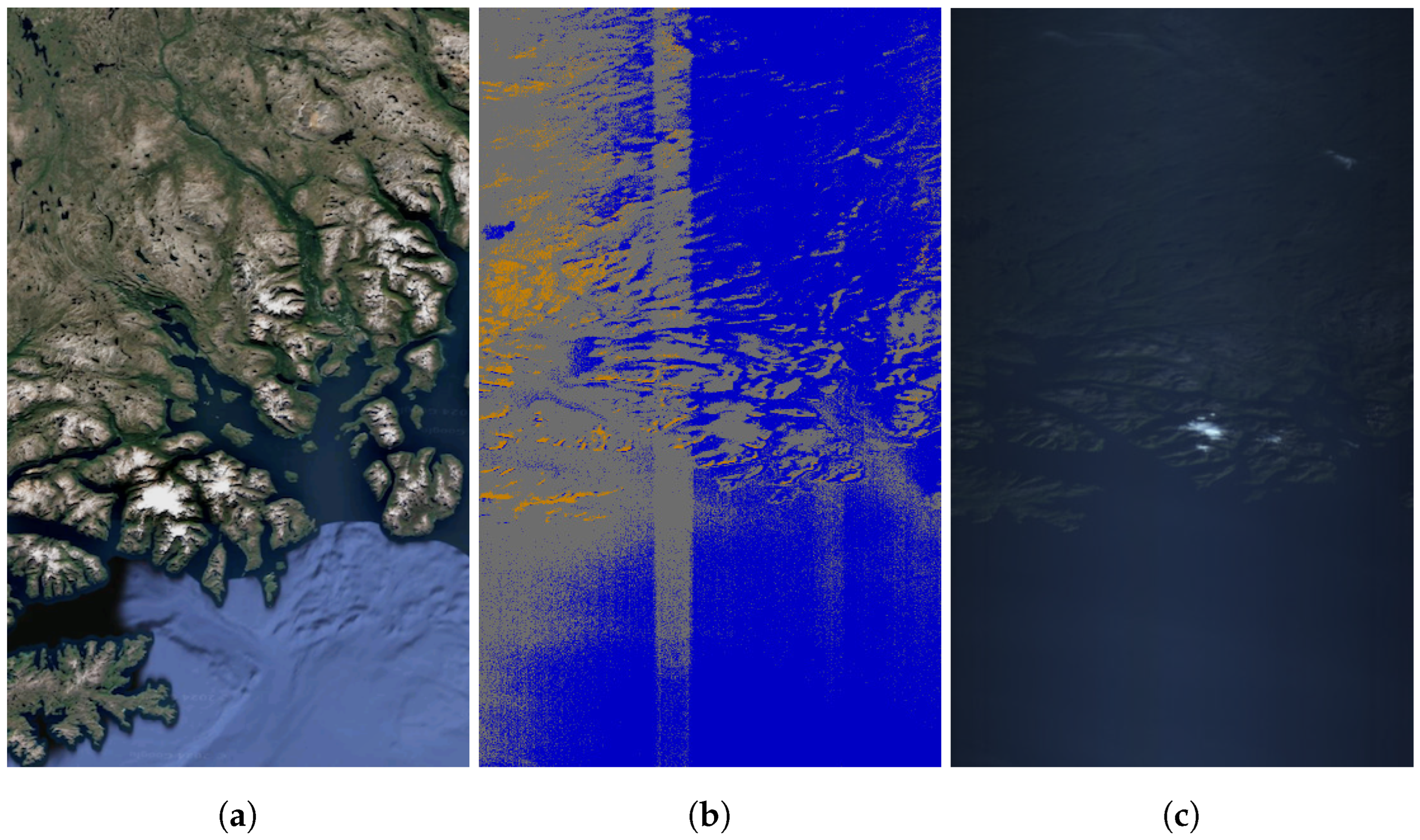
Figure 27.
Finnmark, Norway, Europe, on 21 July 2024 at 18:24 UTC. Coordinates: 70.2° latitude and 22.8° longitude. Solar zenith angle: 79.5°; exposure time: 35 ms. (a) Planned geographical area. (b) Segmented image in orbit. (c) RGB composite from cube.
Figure 27.
Finnmark, Norway, Europe, on 21 July 2024 at 18:24 UTC. Coordinates: 70.2° latitude and 22.8° longitude. Solar zenith angle: 79.5°; exposure time: 35 ms. (a) Planned geographical area. (b) Segmented image in orbit. (c) RGB composite from cube.
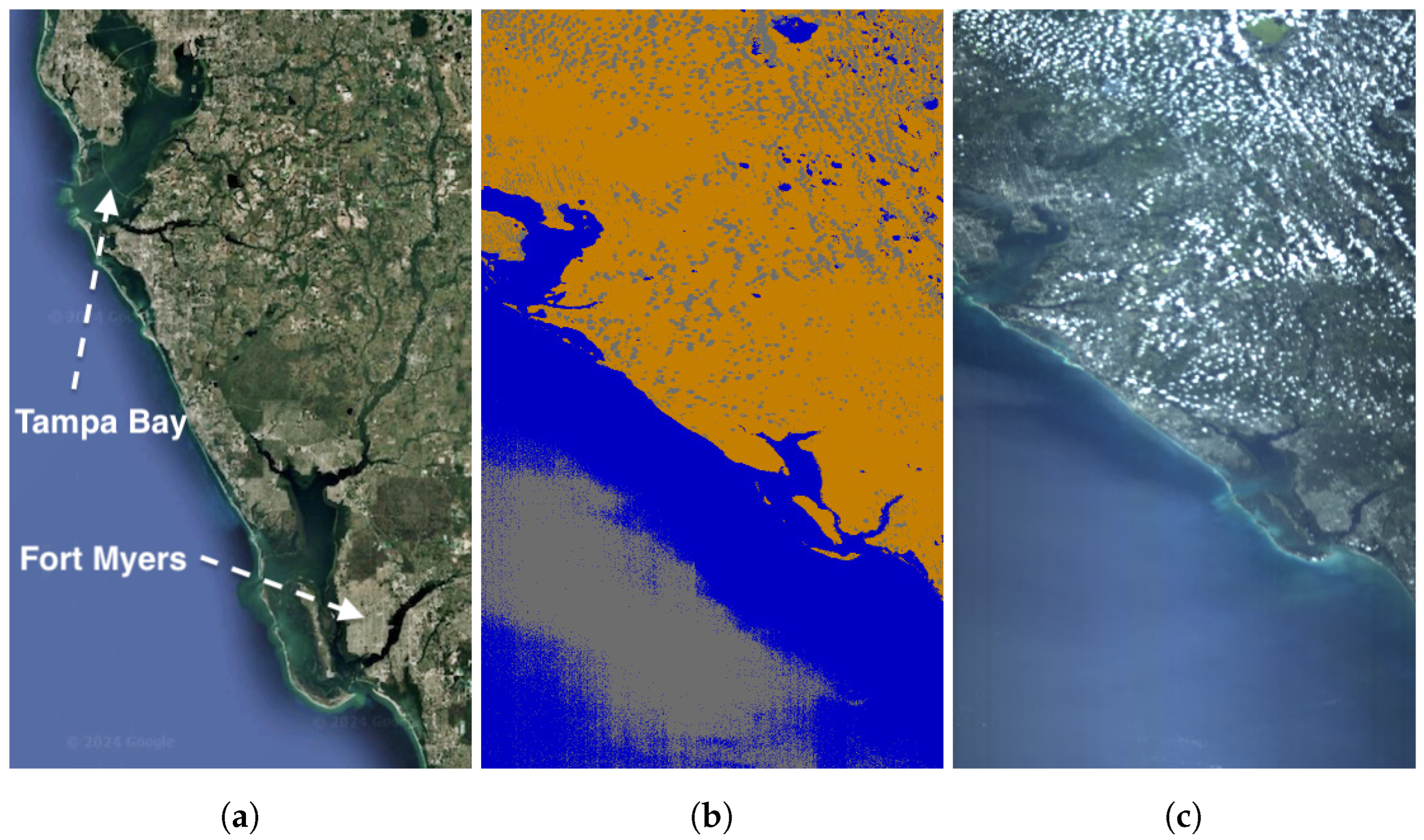
Figure 28.
Florida, USA, North America, on 21 May 2024 at 15:51 UTC. Coordinates: 27.2° latitude and −82.6° longitude. Solar zenith angle: 22.1°; exposure time: 30 ms. (a) Planned geographical area. (b) Segmented image in orbit. (c) RGB composite from cube.
Figure 28.
Florida, USA, North America, on 21 May 2024 at 15:51 UTC. Coordinates: 27.2° latitude and −82.6° longitude. Solar zenith angle: 22.1°; exposure time: 30 ms. (a) Planned geographical area. (b) Segmented image in orbit. (c) RGB composite from cube.
Table 1.
Comparative metrics for segmentation models tested on data from the HYPSO-1 satellite [
39].
Table 1.
Comparative metrics for segmentation models tested on data from the HYPSO-1 satellite [
39].
| Model | Accuracy | Model Size | Inference Time [ms] |
|---|
| 1D-ML/SGD | 0.91 | - | 72 |
| 1D-ML/NB | 0.71 | - | 1234 |
| 1D-ML/LDA | 0.89 | - | 190 |
| 1D-ML/QDA | 0.89 | - | 2024 |
| 1D-Justo-LiuNet | 0.93 | 4563 | 166 |
| 1D-Justo-HuNet | 0.91 | 9543 | 69 |
| 1D-Justo-LucasCNN | 0.91 | 25,323 | 142 |
| 2D-NU-Net-mod | 0.80 | 32,340 | 364 |
| 2D-NU-Net | 0.81 | 40,332 | 374 |
| 2D-CUNet | 0.72 | 67,299 | 272 |
| 2D-CUNet++ | 0.83 | 24,619 | 294 |
| 2D-CUNet Reduced | 0.76 | 22,019 | 270 |
| 2D-CUNet++ Reduced | 0.90 | 12,379 | 294 |
| 2D-UNet FAUBAI | 0.88 | 26,534,211 | 462 |
| 2D-UNet FAUBAI Reduced | 0.85 | 1,956,835 | 388 |
| 2D-Justo-UNet-Simple | 0.92 | 7641 | 318 |
| FastViT-T8 | 0.82 | 5,033,795 | 132 |
| FastViT-S12 | 0.90 | 10,242,819 | 156 |
| FastViT-MA36 | 0.88 | 44,647,755 | 288 |
Table 2.
Comparative metrics comparing 1D-Justo-LiuNet with a 2D-CNN on data from NASA’s EO-1 satellite for generalization [
39].
Table 2.
Comparative metrics comparing 1D-Justo-LiuNet with a 2D-CNN on data from NASA’s EO-1 satellite for generalization [
39].
| Model | Accuracy | F1 Score |
|---|
| 1D-Justo-LiuNet | 0.82 | 0.97 |
| nnU-net 2D | 0.81 | 0.87 |
| 2D-Justo-UNet-Simple | 0.70 | 0.81 |
| 1D-Justo-LiuNet | 0.74 | 0.85 |
| nnU-net 2D | 0.80 | 0.85 |
| 2D-Justo-UNet-Simple | 0.72 | 0.86 |
| 1D-Justo-LiuNet | 0.64 | 0.76 |
| nnU-net 2D | 0.77 | 0.86 |
| 2D-Justo-UNet-Simple | 0.57 | 0.88 |
Table 3.
Notation and descriptions of sequences in 1D-Justo-LiuNet.
Table 3.
Notation and descriptions of sequences in 1D-Justo-LiuNet.
| NOTATION | DESCRIPTION OF THE SEQUENCE |
|---|
| NETWORK’S INPUT |
| Image pixel to be classified, represented by its spectral signature along wavelengths . In this work, each pixel comprises spectral bands. |
| CONVOLUTIONS FOR FEATURE EXTRACTION |
| Weight parameters of the kernels in the convolution layer at level X. Each 2D kernel consists of components across the K dimension. The number of kernel components, , corresponds to the number of kernels used in the convolution at the previous level . Since it is common to use multiple kernels at previous levels, the convolution at level X also demands kernels with multiple components, i.e., . Only at level 1, convolution kernels are, however, single-components (1D) across K as there are no previous convolutions and hence weight parameters are given by . In Table 4, we provide the numerical dimensions for , , and K across 1D-Justo-LiuNet. |
| Bias parameters of the kernels in the convolution at level X. The sequence is always 1D, regardless of whether the kernel weights are multi-component (2D) or single-component (1D). |
| Output sequence of the convolution layer at level X, including all one-dimensional feature maps with length produced by the respective kernels. Each feature map is always one-dimensional regardless of whether the kernel weights are multi- or single-components. |
| POOLING FOR FEATURE REDUCTION |
| Output sequence of pooling layer at level X with feature maps, where their original length is reduced down to . |
| CLASSIFICATION OUTPUT |
| Output sequence of flatten layer representing the I-th highest-level extracted features in the latent space relevant for sea–land–cloud classification. |
| Weight parameters of the C neurons in the dense layer, where C represents the number of classes to detect. Each neuron is fully connected, with I synapses, to the respective features in to calculate the probability that they belong to the neuron’s respective class. |
| Bias parameters of the C neurons in the dense layer. |
| Output sequence of the dense layer (i.e., output of the network), consisting of C class probabilities. |
Table 4.
Overview of the 1D-CNN 1D-Justo-LiuNet showing sequence dimensions.
Table 4.
Overview of the 1D-CNN 1D-Justo-LiuNet showing sequence dimensions.
| INPUT | LAYER PARAMETERS | OUTPUT |
|---|
| SEQUENCE | DIMENSIONS | SEQUENCES | DIMENSIONS | SEQUENCE | DIMENSIONS |
| FEATURE EXTRACTION AND REDUCTION |
| LEVEL 1 |
| CONVOLUTION ( kernels; ) |
| 1 × 112 | | 6 × 6 | | 6 × 10⁷ |
| | | | 1 × 6 | | |
| POOLING |
| 6 × 10⁷ | N/A* | N/A | | 6 × 53 |
| LEVEL 2 |
| CONVOLUTION ( kernels; ) |
| 6 × 53 | | 12 × 6 × 6 | | 12 × 48 |
| | | | 1 × 12 | | |
| POOLING |
| 12 × 48 | N/A | N/A | | 12 × 24 |
| LEVEL 3 |
| CONVOLUTION ( kernels; ) |
| 12 × 24 | | 18 × 12 × 6 | | 18 × 19 |
| | | | 1 × 18 | | |
| POOLING |
| 18 × 19 | N/A | N/A | | 18 × 9 |
| LEVEL 4 |
| CONVOLUTION ( kernels; ) |
| 18 × 9 | | 24 × 18 × 6 | | 24 × 4 |
| | | | 1 × 24 | | |
| POOLING |
| 24 × 4 | N/A | N/A | | 24 × 2 |
| FLATTENING OF FEATURES |
| 24 × 2 | N/A | N/A | | 1 × 48 |
| CLASSIFICATION OF FEATURES |
| DENSE ( class neurons to 48-dimensional latent space) |
| 1 × 48 | | 3 × 48 | | 1 × 3 |
| | | | 1 × 3 | | |
Table 5.
Classification of segmented images based on confidence probability.
Table 5.
Classification of segmented images based on confidence probability.
| SEGMENTED IMAGES | PROBABILITY | CATEGORICAL PREDICTION |
|---|
| Figure 6b | (1.00, 0.00) | no mispointing |
| Figure 9b | (0.00, 1.00) | mispointing |


 ,
, 

