Multipath Effects Mitigation in Offshore Construction Platform GNSS-RTK Displacement Monitoring Using Parametric Temporal Convolution Network

Abstract

The Global Navigation Satellite System (GNSS), renowned for its high precision and automation, has shone brightly in the deformation monitoring of offshore facilities and sea-crossing bridges. However, antennas placed in these locations are often subject to signal interference from various reflective surfaces, such as rivers and oceans, which significantly compromises observation accuracy and reliability. Synthesizing previous research, we first propose a method for multipath dataset construction, which involves GNSS observation linear combinations, detailed mapping of the near-field reflector, and employed static solution residuals as reference. Subsequently, we construct and train a corresponding para-TCN (parametric Temporal Convolution Network) to enable real-time prediction of multipath prediction. Through time domain and frequency domain analysis, it has been demonstrated that the trained network can capture the main features of multipath models and suppress those components in both the data distribution and frequency band, effectively mitigating the interference of multipath errors in observations.

1. Introduction

The Global Navigation Satellite System (GNSS), due to its precise positioning, high automation, and long-term stability, is widely employed in three-dimensional deformation tasks for bridges and other water-based infrastructures. Currently, GNSS has achieved remarkable monitoring results in tasks such as natural frequency extraction [1,2], dynamic deformation monitoring [3,4,5,6,7], tower movement monitoring [8,9], and long-term settlement measurement, aiming to ascertain the operational status of bridges [10], monitor any potential damage, and provide data support for maintenance personnel to intervene. The positioning process of GNSS, which correlates station–satellite distances with time using the speed of light, constitutes a continuous effort to eliminate observation errors in order to achieve higher positioning accuracy. Notably, among the resolution methods, the Real-Time Kinematic (RTK) method stands out in monitoring water-based infrastructure due to its centimeter-level accuracy, ease of deployment, and swift response. The RTK method employs the double difference between satellites and stations to eliminate common errors caused by satellite and receiver clock biases. When the baseline is sufficiently short, it can significantly mitigate troposphere and ionosphere errors by leveraging the consistency of satellite signal propagation paths.

However, despite its ability to eliminate the most common errors, the RTK method remains helpless against multipath interference caused by variations in the near-field environment of rover and base stations; actually, multipath errors have already become the primary source of errors in dynamic bridge monitoring [11,12]. Multipath effects occur when the satellite signals received by the GNSS antenna are no longer solely direct signals but rather composite signals formed by the superposition of direct signals and reflected (or refracted) signals excited by multiple reflection sources [13]. The difference between the composite signal and direct signal leads to positioning error, namely multipath error.

Presently, the RTK method employs carrier phase observations for positioning solutions when utilizing ancillary techniques such as near-field environment perception. In order to achieve real-time multipath error elimination, SNR and pseudorange observations have gained widespread use in urban canyon positioning [14] and multipath interference identification [15,16] due to their pronounced multipath components and the tedious ambiguity resolution (AR) process, which is an unavoidable step in precise carrier-phase positioning methods. Because carrier multipath components have a rapid phase-change frequency, and the maximum amplitude of the carrier multipath is only one-fourth of the corresponding wavelength (for GPS L1 frequency band with a wavelength of 19.03 cm, this value is approximately 4.76 cm), a precise multipath identification requires a centimeter-level estimation of both antenna position and reflector position; otherwise, the mitigation errors can become extremely large (as we would specifically illustrate in Section 2.1).

The multipath mitigation approaches for carrier-based positioning predominantly hinge on near-field sensing and filtering techniques. In the context of structural monitoring, given the invariance of the near-field environment, the amplitude and phase of multipath signals are solely associated with the directional vector between the observer and satellite, facilitating their direct representation on a multipath hemispherical map (MHM) [17,18] that consists of grids. An MHM grid exhibiting severe multipath errors can be subjected to weighting reduction or discarding, considering the high susceptibility that strong reflectors exist in those directions. While the MHM method boasts favorable real-time capabilities, its effectiveness is challenged in environments with fluctuating water levels, and it requires a relatively long period of observation to fulfill the grid map. Another widely employed post-processing technique is Sidereal Filtering (SF) [19,20,21,22]. SF firstly builds satellite observation residuals from pure static measurement on a given day, extracts their multipath characteristics, then removes the corresponding satellite’s multipath signatures over the ensuing sidereal days. Unfortunately, water level variations essentially constitute a dynamic near-field environment, and the accuracy achieved through direct residual differentials is often unsatisfactory under that circumstance.

Nevertheless, multipath effects do not always have a negative impact. Researchers have placed GNSS antennas in locations such as shore-based stations [23,24,25] and lighthouses [26], treating the surrounding water areas as signal reflectors to capture the multipath components within the Signal-to-Noise Ratio (SNR) [27] and linear combinations of observations [16], then inversely calculated the height difference between the antenna and the water surface. In recent years, with the enhancement of carrier observation accuracy, combinations of carrier phase observations have also been included to identify the dynamic reflector source [28,29], primarily relying on spectrum analysis for the recognition task. In summary, these efforts employ static single-receiver observations, and identify the reflector location by spectrum analysis.

These works offer valuable insights, demonstrating that when a reflect source within a given time window can be uniquely identified, then multipath components present in both pseudorange and carrier phase observations during that period can also be uniquely determined. Since pseudorange and carrier phase measurements constitute distinct frequency components of the same signal, they experience coherent reflection from common surfaces and, based on theoretical derivations, exhibit analogous spectral characteristics. This establishes the theoretical foundation for our model, which utilizes multipath components in pseudorange and carrier observations to circumvent the complex and error-prone integer ambiguity resolution process. By directly performing residual filtering on the output of RTK Kalman filter, we can eliminate the multipath components in the positioning equations without resolving, thereby improve the accuracy of GNSS positioning.

Building upon the relationship between multipath signals and their connection in the near-field environment, alongside the intricate linkage combined with pseudorange and carrier phase multipath interconnections, we have developed a neural network designed for real-time mitigation of multipath interference through multipath signature dataset development. The following sections would elaborate on the detailed implementations:

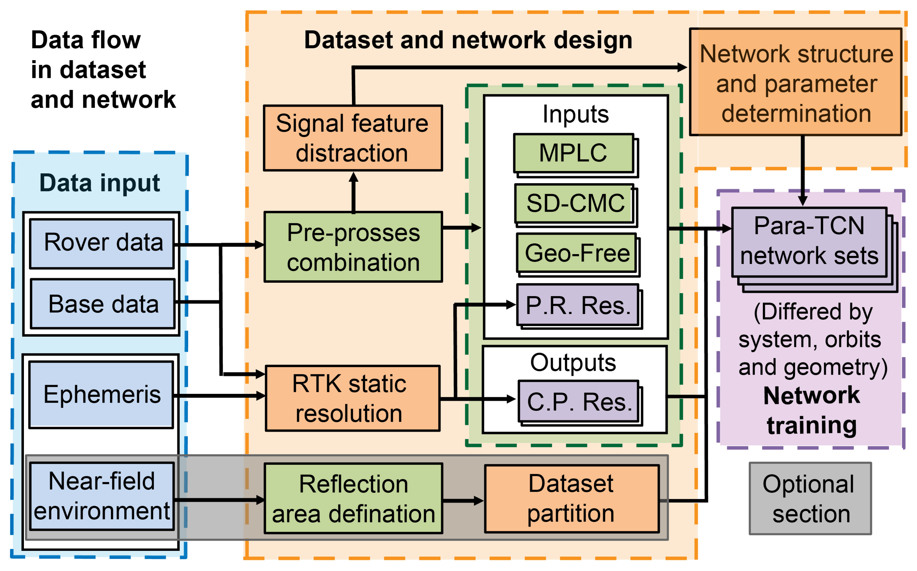
• Section 2 conducts a systematic analysis of the generation mechanism of multipath signals within offshore construction platform environments, linking multipath signatures to structural geometries present in near-field environments. By systematically processing pseudorange and carrier phase signals collected from GNSS receivers, one could derive analytical expressions for the network inputs parameters under constrained dual-frequency/dual-station configurations. After formulating those observations into dataset, based on rigorous characterization of multipath propagation, we presented the neural network employed for multipath prediction, accompanied by detailing the architectural selections for network layer configurations and hyperparameters.
• Section 3 quantitatively evaluates the effectiveness of our neural network predictions, demonstrating the multipath mitigation performance across test subsets with signal-domain metrics including temporal distribution analysis and spectral power quantification, yielding a holistic validation framework.
• Section 4 systematically examines dataset preprocessing/normalization strategies, explainable of network parameter settings, andreflection-source-informed skymap segmentation.

2. Materials and Methods

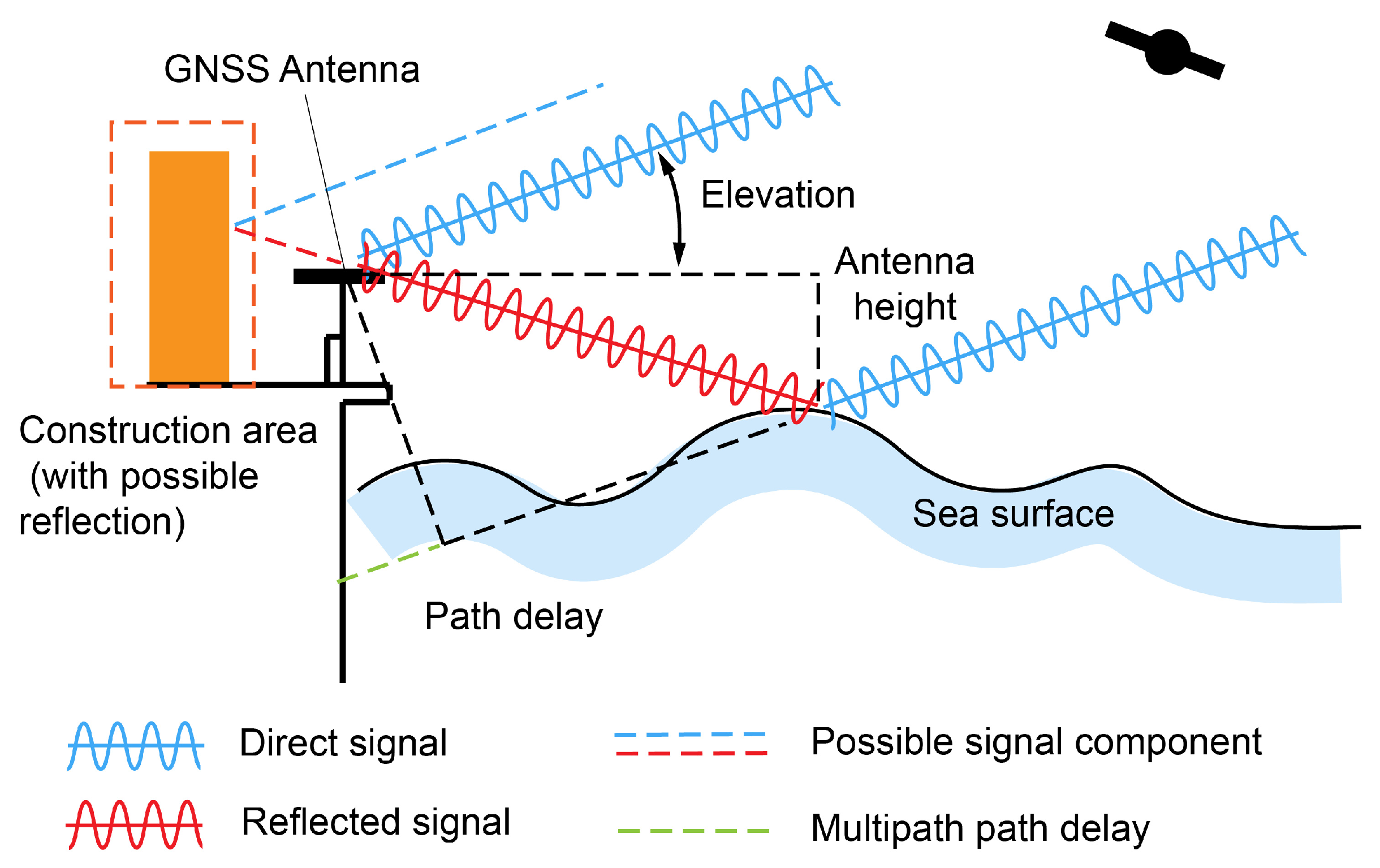
2.1. Geometry of GNSS Multipath Effect

The multipath component in GNSS observations refers to the fact that, besides the direct signal, the receiver also captures non-direct signals from the same satellite. Since non-direct components possess the same frequency, the receiver ultimately obtains a composite signal that includes various components [13]. As shown in Figure 1, a satellite signal travels from the far field, undergoes near-field environmental effects (usually reflection), and is then received by the antenna. The facility has horizontal panels and certain vertical obstructions (these obstructions are likely to be fixed on bridges but may change on offshore construction platforms), and there is ocean on the other side. Signals traveling from the sea direction is affected by multipath reflections from the sea surface, while the signal traveling from the structure direction may be affected by structural reflections, although the reflection strength from the structure is much weaker compared to the sea surface.

Also in Figure 1, given that the monitoring object is an offshore construction platform or a sea-crossing bridge, a GNSS antenna is typically positioned at platform edge to avoid construction conditions or maintain traffic clearance. Therefore, a significant number of these antennas experience multipath effects predominantly caused by ocean surface reflection. As noted by Zhang [23] and Roussel [26], although the water level remains stable over a long period of time, its transient fluctuations induce variations in the path delay $\Delta s$, the defining geometric parameter for multipath phenomena. Using path delay, the I/Q vector-gram comparing original, multipath and the composite signals is plotted in Figure 2 [30], where S stands for signal, subscripts d, m and c representing direct, multipath and composite components, respectively. The phase difference $\psi$ between $S_d$ and $S_m$ varies as a function of path delay $\Delta s$, thus the phase offset $\delta \varphi$ between $S_d$ and $S_c$ is characterized by Equations (1) and (2) [31]:

$$\delta \phi =arctan\left({\displaystyle \frac{A_{d}sin\psi }{A_d+A_{m}cos\psi }}\right)$$

(1)

$$\psi ={\displaystyle \frac{2\pi }{\lambda }}\Delta s=\left(2\pi {\displaystyle \frac{2H}{\lambda }}sin\epsilon \right)$$

(2)

where $|A_d|$ and $|A_m|$ are the amplitude of original and multipath signal, $\lambda$ is the corresponding wavelength, H stands for the height difference between GNSS antenna and the reflection point, and $\epsilon$ is the satellite elevation. Because carrier phase measurement generate its observation by phase counting, the phase difference between composite and original signal can be directly regarded as the additive carrier phase multipath, ${\mathrm{MP}}_{\mathrm{L}}$. For pseudo-range measurement, multipath component ${\mathrm{MP}}_{\mathrm{P}}$ is derived by multiplying path delay with the reflection coefficient $\alpha =A_m/A_d$, under the assumption that $\alpha$ is much smaller than 1 [23].

$$\mathrm{M}{\mathrm{P}}_{\mathrm{L}}={\displaystyle \frac{\lambda }{2\pi }}arctan\left({\displaystyle \frac{\alpha sin\delta \phi }{1+\alpha cos\delta \phi }}\right)$$

(3)

$$\mathrm{M}{\mathrm{P}}_{\mathrm{P}}={\displaystyle \frac{2H·sin\epsilon ·\alpha ·cos\delta \phi }{1+\alpha cos\delta \phi }}$$

(4)

Since carrier-phase multipath effects are governed by coefficient $\lambda /2\pi$, it becomes evident that the amplitudesignificantly exceed those of carrier-phase components. This occurs because path delay primarily impacts ${\mathrm{MP}}_{\mathrm{L}}$ through phase modulation, while exhibiting linearly correlated with ${\mathrm{MP}}_{\mathrm{P}}$ magnitude. In fact, Hofmann [32] pointed out that the carrier-phase multipath limitation is bounded to one-quarter wavelength, whereas the ${\mathrm{MP}}_{\mathrm{P}}$ values in urban-canyon environments may sometimes exceed morethan 10 m. For water-surface reflections, the amplitude of ${\mathrm{MP}}_{\mathrm{P}}$ typically remains within 0.5 m, exhibiting fluctuations of 0.1–0.2 m [23].

2.2. GNSS Observation and Multipath Dataset

2.2.1. GNSS Observation

In the context of positioning algorithms, the primary observations consist of pseudorange and carrier phase measurements; combined with the navigation data, these three frequency-differentiated signal components form a complete transmission from satellites on designated frequencies. The pseudorange and carrier phase observations from satellite s within frequency band $L_i$ received at station r could be expressed in Equations (5) and (6) as [33]:

$$\begin{array}{c}\hfill P_{r,i}^s={\rho }_r^s+c\left(d{t}_r-d{T}^s\right)+I_{r,i}^s+T_r^s+{\mathrm{MP}}_{r,i,\mathrm{P}}^s+\epsilon (0,{\sigma }_{\mathrm{P}}^2)\end{array}$$

(5)

$${\mathrm{\Phi }}_{r,i}^s={\lambda }_i{\varphi }_{r,i}^s={\rho }_r^s+c\left(d{t}_r-d{T}^s\right)-I_{r,i}^s+T_r^s+{\lambda }_i{B}_{r,i}^s+{\mathrm{MP}}_{\mathrm{r},\mathrm{i},\mathrm{L}}^{\mathrm{s}}+\epsilon (0,{\sigma }_{\mathrm{L}}^2)$$

(6)

Both observations contain errors originating from satellite signal propagation path as well as satellite/receiver hardware imperfections. High-precision positioning methods primarily utilize carrier phase observations due to their superior precision compared to pseudorange measurements, though they exhibit greater susceptibility to multipath effects during the ambiguity resolution (AR) process required to obtain fixed solutions.

When multipath is modeled as an additive error in the observation equation as listed in Equation (1), it persists in differential models due to its strong correlation with the receiver’s near-field environment. To enable neural network multipath prediction, we construct three linear combinations of GNSS observations as input sequences isolating multipath signatures, achieved by eliminating or fixing other components as constants through differential models. Crucially, rover station positions are removed in these combinations, rendering small displacements irrelevant to the preserved multipath components. Furthermore, We assume a fixed base station antenna with minimal multipath per construction standards.

2.2.2. Multipath Observation Dataset

The followings are linear combinations of the observations used for multipath mitigation, while multipath in each observation is modeled as additive.

The Code-Minus-Carrier (CMC) values are typically adopted to evaluate the strength of multipath within an observation [15,16]. However, CMC data from a single receiver suffers severe ionospheric and tropospheric delays, requiring these delays to be treated as constants for interference removal. Relying on the presence of base stations, we employ single-difference (SD) CMC as a proxy for CMC to satisfy dataset requirements, that common errors must be eliminated, and all other components besides multipath shall be constrained as constants.

$$\begin{array}{cc}\hfill {\mathrm{CMC}}_{rb,i}^s& =\left(P_{r,i}^s-P_{b,i}^s\right)-\left({\mathrm{\Phi }}_{r,i}^s-{\mathrm{\Phi }}_{b,i}^s\right)\hfill \\ \hfill & =I_{rb,i}^s+T_{rb}^s+{\lambda }_i{B}_{rb,i}^s+{\mathrm{MP}}_{rb,i,\mathrm{P}}^s+{\mathrm{MP}}_{rb,i,\mathrm{L}}^s+\epsilon (0,2{\sigma }_{\mathrm{P}}^2+2{\sigma }_{\mathrm{L}}^2)\hfill \end{array}$$

(7)

Compared to CMC observations, the multipath linear combination (MPLC) utilizes dual frequency signals from the same satellite to eliminate the ionospheric delay [34]. Its advantage lies in providing stable values over extended periods without reference station assistance. However, because it requires dual-frequency observations, MPLC introduces multipath effects from the secondary frequency due to its dual-frequency requirement, with carrier-phase multipath components being non-uniformly scaled by coefficient $k_{ij}=f_i/f_j$.

$$\begin{array}{cc}\hfill {\mathrm{MPLC}}_{r,i}^s& =\left(P_{r,i}^s-{\mathrm{\Phi }}_{r,i}^s\right)-{\displaystyle \frac{2}{k_{ij}-1}}\left({\mathrm{\Phi }}_{r,i}^s-{\mathrm{\Phi }}_{r,j}^s\right)+{\displaystyle \frac{2}{k_{ij}-1}}\left({\lambda }_i{B}_{r,i}^s-{\lambda }_i{B}_{r,j}^s\right)\hfill \\ \hfill & {\mathrm{MP}}_{r,i,\mathrm{P}}^s-{\displaystyle \frac{k_{ij}+1}{k_{ij}-1}}{\mathrm{MP}}_{r,i,\mathrm{L}}^s+{\displaystyle \frac{2}{k_{ij}-1}}{\mathrm{MP}}_{r,j,\mathrm{L}}^s+\mathrm{Consts}.+\epsilon (0,{\sigma }_{\mathrm{P}}^2+{\displaystyle \frac{k_{ij}+1}{k_{ij}-1}}{\sigma }_{\mathrm{L}}^2)\hfill \end{array}$$

(8)

In establishing these two linear combinations, SD-CMC employs reference stations for error mitigation, while MPLC removes ionospheric delays via dual frequencies. We thus introduce a pure carrier phase combination involving rover/reference stations and ionospheric delays to bridge both methods, while remaining insensitive to minor rover displacements. The geometry-free measurement [35,36] is selected as this third component, as it is often used in cycle slip detection and is formed based on the presumption that ionospheric total electronic content (TEC) varies little in short terms.

$$\begin{array}{cc}\hfill {\mathrm{GF}}_{rb,ij}^s& =\left({\mathrm{\Phi }}_{r,i}^s-{\mathrm{\Phi }}_{b,i}^s\right)-\left({\mathrm{\Phi }}_{r,j}^s-{\mathrm{\Phi }}_{b,j}^s\right)\hfill \\ \hfill & =-\left(I_{rb,i}+{\lambda }_i{B}_{rb,i}^s\right)+\left(I_{rb,j}+{\lambda }_i{B}_{rb,j}^s\right)+{\mathrm{MP}}_{rb,ij,\mathrm{L}}^s+\epsilon (0,4{\sigma }_{\mathrm{L}}^2)\hfill \end{array}$$

(9)

2.2.3. Real-Time Code-Aided Multipath Mitigation

In prior work [37], we extracted pseudorange/carrier multipath via phase alignment and iterative optimization to suppress correlated components. While post-processing revealed frequency-domain correlations, this paper focuses on real-time mitigation, necessitating hardware adaptations for onboard computation/storage. This data preparation workflow is summarized in Figure 3.

The flowchart is structured into two distinct modules: the upper neural network governed section and the lower conventional RTK processing pipeline. The neural network fuses current epoch inputs with historical data to form a new set of input sequences. These sequences—stratified by satellite, system, orbital parameters, and environmental geometry—are processed through dedicated prediction networks. Predicted multipath components are then supplied to a secondary RTK-Kinematic iteration for residual mitigation, while obsolete epoch data are purged to accommodate incoming observations.

The RTK module first formats dual-station observations into differential combinations, which are simultaneously appended to neural network inputs. Crucially, the initial RTK employs static-mode processing, where pseudorange residuals inform neural network multipath corrections. Subsequent carrier phase residuals—after multipath mitigation- are propagated to the secondary RTK module for dynamic displacement estimation. Both stages maintain operational independence, autonomously preserving their computational states.

2.3. Dataset Acquisition and Data Property Driven Partition

This section describes how the linear combinations of GNSS observations are structured into a multipath-aware dataset, organized according to data processing sequences and neural network workflows. We begin by providing a concise overview of dataset acquisition (given prior elaboration of linear combinations), followed by explanations for partitioning the dataset for specialized applications. Based on inherent data distributions, we determine neural network parameters and architectures. Figure 4 summarizes the data flow.

The methodology focuses on acquired GNSS data, emphasizing dataset attributes and characteristics. An ideal dataset exhibits prominent input/output features (i.e., high signal-to-noise ratios) and strongly correlated inter-data relationships. Crucially, systems with distinct parameters must be analyzed separately—as emphasized by Wang et al. [38], demonstrating that system variations (e.g., BOC (Binary Offset Carrier) vs. BPSK (Binary Phase Shift Keying) signals) yield divergent multipath characteristics. We first analyze satellite counts per system to assess dataset distribution.

As shown in Figure 5, Beidou GEO/IGSO satellites exhibit prolonged observation durations compared to MEO counterparts. Effectively mitigating GEO/IGSO multipath significantly improves positioning accuracy due to their dominant data volume. However, GEO satellites’ minimal sky track movement complicates multipath characterization, as static elevations may preclude time-dependent periodicity. This study solely focuses on GPS MEO, BeiDou MEO, and IGSO satellites.

Figure 5 compares total data volumes, revealing that despite fewer GEO/IGSO satellites than MEO counterparts, persistent orbital presence yields comparable data quantities across all four categories. The left subfigure statistically represents dataset properties, with horizontal axes denoting sequence IDs and vertical axes recording durations, highlighting GEO/IGSO data density. To optimize multipath modeling, we implement architecturally identical networks trained on segregated datasets, enhancing multipath interference suppression.

2.4. Data Sources and Reliability

The environment perception and data collection of this work were conducted in the Dongwuyang sea-crossing bridge located in Xiapu, Ningde, Fujian Province, approximately 119°56′51″ E, 27°39′4″ N. As shown in Figure 6, GNSS antennas are edge-mounted due to platform constraints. While geometric parameters are readily measurable, we establish elevation thresholds (e.g., 15°) to derive maximum azimuth offsets via trigonometric relationships, determining sea-reflection regions. Since multipath characteristics depend on reflecting media, isolating surfaces by material constitutes a viable approach (see Section 4 implementation in Figure 4 gray box).

Following data-type segmentation, we define sequence segmentation criteria: observation breaks (e.g., satellite signal loss-of-lock) mark dataset discontinuities due to disrupted carrier-phase continuity. Temporary residual interruptions, however, do not constitute segmentation points under static positioning conditions, as a static resolution ensures the continuous nature of the measurement location. Dataset construction details are elaborated in Section 4.

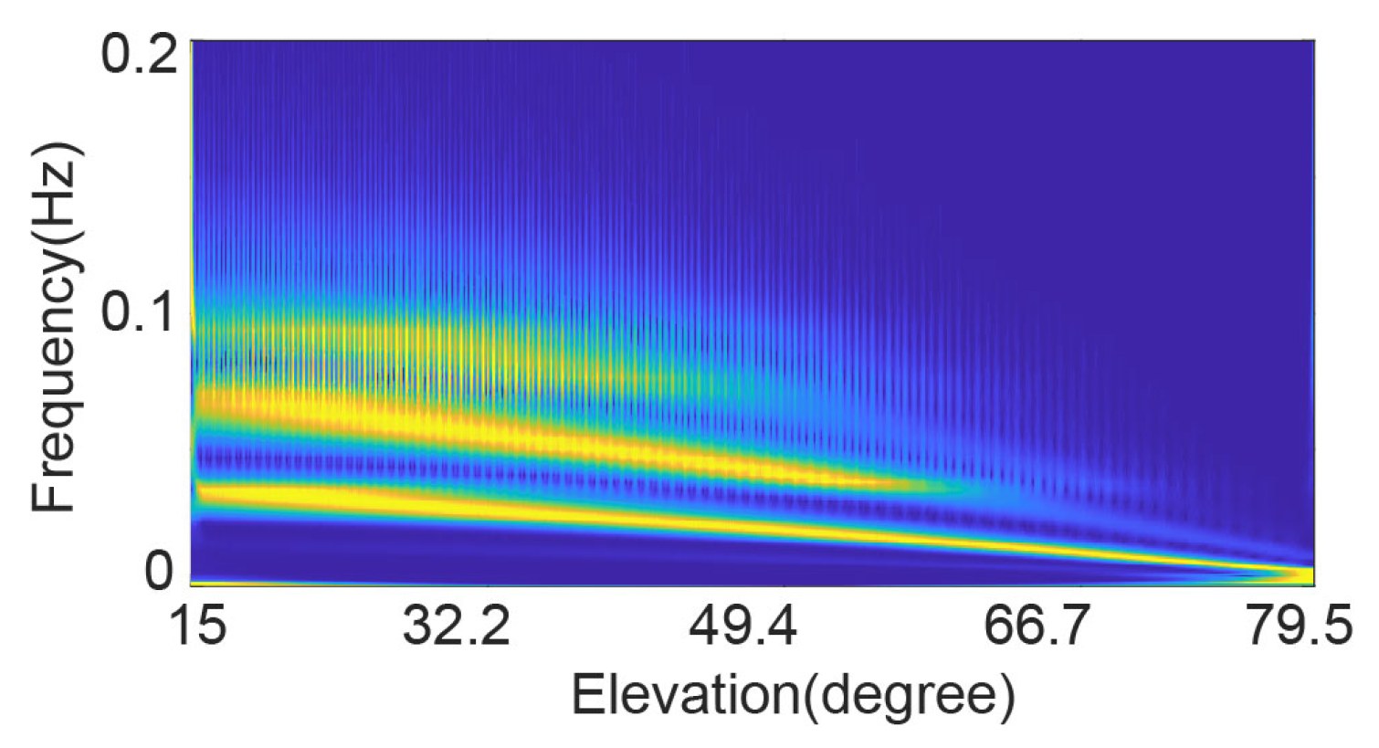
2.5. Characteristics of GNSS Multipath

For GNSS devices, all multipath inputs and satellite-specific residuals constitute time-series data, necessitating a sequence-to-sequence regression framework. As Equations (3) and (4) indicate, multipath’s additive nature manifests as low-frequency components. Figure 7 illustrates this via code multipath’s Continuous Wavelet Transform, with 0.029 Hz dominant frequency at 15° elevation. Harmonic effects introduce secondary/tertiary frequencies, complicating analysis by broadening the spectral profile. Thus, the network must simultaneously resolve stable long-period baseband multipath and detect high-frequency harmonics.

Traditional sequential processing architectures including recurrent neural networks (RNNs), long short-term memory (LSTM), and gated recurrent units (GRUs) are constrained by their inherent network topologies that prohibit parallelized training procedures. When real-time state variable updates are progressively executed with temporal evolution, the capacity for capturing long-term temporal dependencies is fundamentally constrained. Moreover, augmenting the parameter count to improve prediction fidelity induces exponential growth in computational complexity, thereby substantially elevating the optimization challenge.

To mitigate these limitations, hybrid architectures such as the CNN-LSTM framework convert temporal signals obtained through conventional time-frequency analysis into two-dimensional representations. This modality transformation strategy exploits the complementary benefits of convolutional feature abstraction and parallel computation capabilities. However, the inevitable information degradation during transformation processes continues to impose restrictions on network accuracy enhancement.

The Transformer architecture [39] has fundamentally transformed natural language processing (NLP) paradigms through its exclusive reliance on self-attention mechanisms, displacing conventional RNN and CNN approaches. Notwithstanding these advantages, the architecture mandates supplementary temporal embedding operations for time-series analysis and exhibits substantial data dependency during parameter estimation phases [40]. Furthermore, significant hardware resource requirements for implementation pose particular challenges for civilian-grade receiver deployments.

2.6. Parallel Temporal Convolution Network

Given the critical constraints of hardware implementation costs, training efficiency, and model interpretability, the temporal convolution network (TCN) [41] was adopted as the foundational architecture for sequential data processing in this study. The TCN architecture is characterized by its capability to process temporal sequences through causal convolution operations, with three defining attributes:

• Causal convolution, where the output at a given time step can only be calculated using information from previous time steps.
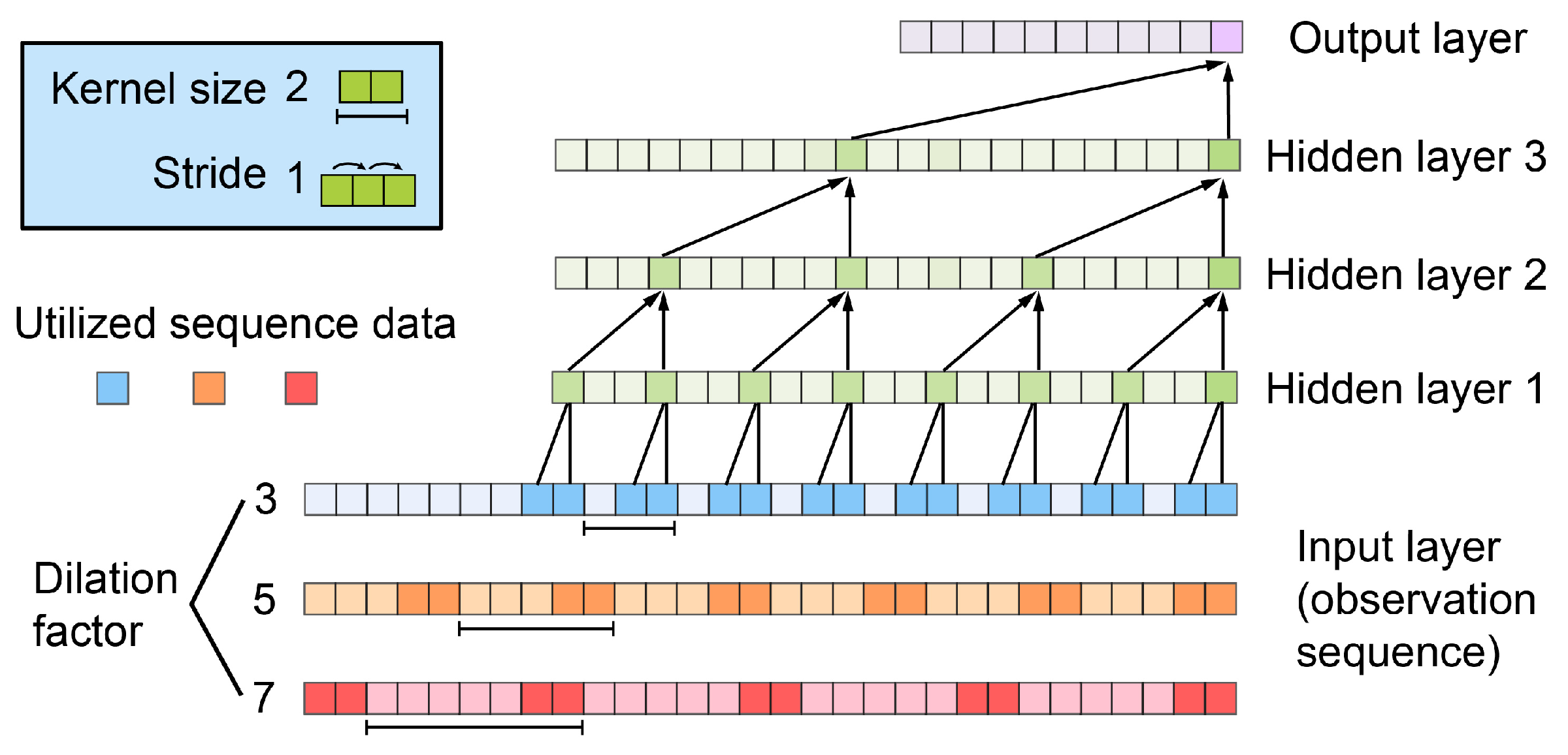
• Dilated convolution, which expands the receptive field by adjusting the dilation factor of the convolution kernel, allowing a single convolution kernel to capture features from longer sequences.
• Interpretability, that whether a node is being used or not can be obtained through the inverse inference of the network structure, and the data flow within the network can be finely modeled.

When prior knowledge exists regarding the principal component frequency bands of input signals, the filter configuration can be directly customized through architectural modifications.

Building upon TCN’s inherent logical structure, Fan et al. [42] developed a prefix-based spatiotemporal attention module to capture cross-channel correlations. This approach employed dual parallel TCN backbones with stacked dilation layers, resulting in enhanced predictive performance through temporal feature fusion. The parametric architecture paradigm was further implemented in SLNet [43], which incorporated multimodal signal processing strategies by applying short-time Fourier transform (STFT) operators with heterogeneous time-frequency resolutions. The resultant spectrograms were processed through parallel network pathways for feature extraction and decision fusion, demonstrating superior accuracy and computational efficiency compared to conventional temporal architectures.

Drawing from these methodological advancements, our architecture integrates multiple TCN backbones with identical structures but varying dilation factors. Each backbone is augmented with dedicated fully-connected layers, subsequently combined through a parametric fusion mechanism to construct the complete parallel TCN framework. The comprehensive network topology is illustrated in Figure 8.

2.7. Network Structure Design

The explicit data flow architecture of TCN enables precise structural adaptation. Consider a TCN backbone comprising 3 hidden layers with stride 1 and convolution kernel size 2, where the dilation factors are configured as 3, 6, and 12 respectively. This configuration establishes an effective receptive field spanning 24 nodes, equivalent to processing input nodes with a skip 1 for every 2 nodes at the input end for8 rounds, as illustrated in the input layer of Figure 8. Modifying the dilation factors effectively alters the relative positioning of input nodes (excluding overlapping regions) for prediction, analogous to multi-rate sampling of the original sequence. Optimal coverage of input nodes through this mechanism enhances prediction accuracy.

From a signal processing perspective, each TCN backbone with unique dilation factors implements a distinct down-sampling operation on the input data. As demonstrated in

Table 1. Parameters of network and dataset.

Parameters	Value/Data	Notes
Solver	Adam
Kernel size	5	No less than
Stride	1
Dilation factors	[2, 5, 8, 13, 17, 21]	stacked 6 times
Window size	600 (s)	No less than
Sample rate	1 Hz	Rover & Base
Train/Validation set	90%/10%	# of sequences

, using a baseline kernel size of 5, the three-layer backbone structure processes 125 original input points (excluding overlaps) in each parallel TCN channel, enabling multi-scale feature extraction from the original sequence.

In summary, the task of adjusting the dilation factors across channels bears some resemblance to determining the frequencies at various levels in the DWT (Discrete Wavelet Transform) process, albeit the frequencies in DWT algorithm are given in dyadic scales. To achieve a finer frequency resolution without unduly burdening network training, the dilation factors selected for the network design are slightly interpolated and adjusted based on dyadic scales, resulting in a set of para-TCN pathways that balance both high and low-frequency features. Also noted that, in this task, adding more parallel pathways may not necessarily lead to significant improvements in accuracy, but will undoubtedly incur additional computational resources for network training and require a larger amount of dataset; except for the dilation factor, other hyper-parameters in this work are preset to fixed values. More detailed decisions could be referred in Section 4.

3. Results

Given that the principal component of the input data corresponds to multipath effects and considering the measurement points on the platform remain stationary, the static computation mode enables the treatment of multipath interference as the dominant component in carrier phase residuals. This assumption holds particularly for short baselines, where other common error sources are sufficiently mitigated to be considered negligible. Within this framework, the trained network generates real-time predictions of multipath effects for each epoch. The prediction accuracy directly correlates with the network’s efficacy in multipath error mitigation.

It should be noted that the present study focuses specifically on the correction of carrier phase residuals through neural network implementation. The resulting positioning accuracy, derived from these mitigated residuals, represents an extrapolated outcome. Building upon our previous work [37], which established the correlation between multipath mitigation in carrier residuals and positioning accuracy enhancement, the current verification process concentrates on the analysis of positioning residual sequences.

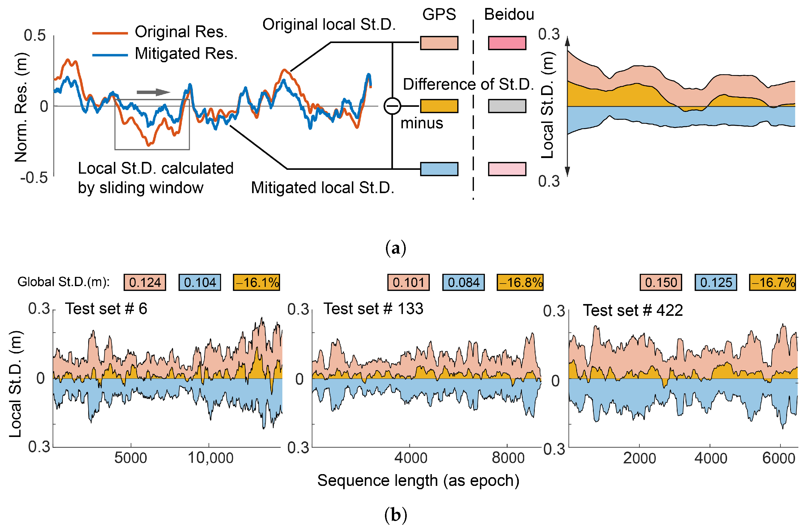
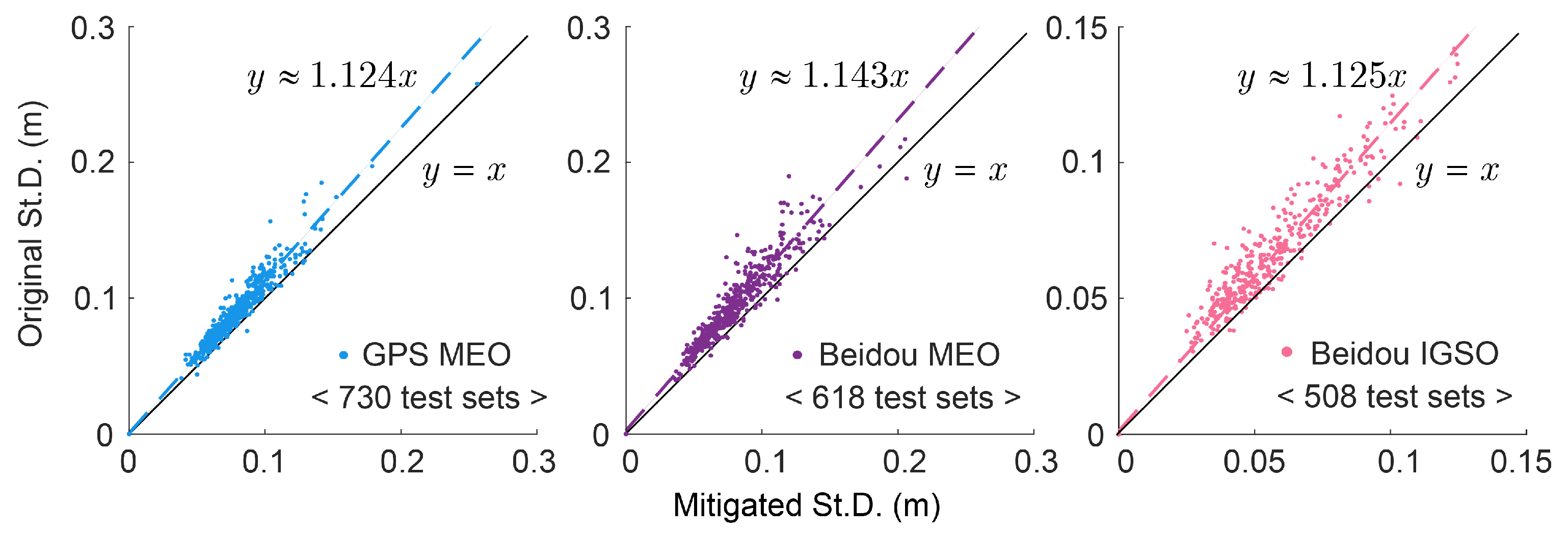
3.1. Multipath Mitigation for Individual Satellite

The input and output sequences in the dataset were pre-processed through moving average removal, employing a window size consistent with the specifications in Table 1 conform to real-world measurement conditions. In practical monitoring scenarios, these moving averages can be efficiently computed in real-time through buffer-based incremental updates. The processed data is subsequently fed into the pre-trained network for real-time correction. Initial results demonstrating these corrections are presented in Figure 9 to provide intuitive understanding of the network’s performance.

Figure 9 demonstrates the instantaneous distribution changes before and after network processing. As shown in Figure 9a, a 180-s sliding window was employed to calculate local standard deviation (St.D.) at each temporal point, generating instantaneous distribution curves through connection of these values. The differential between Original and Mitigated curves represents the intermediate distribution, illustrating the reduction in data dispersion. Global St.D. values, recorded above each subplot, demonstrate the percentage reduction achieved through mitigation. These distribution characteristics reveal the network’s capability to mitigate multipath effects through data distribution smoothing, with positive mitigation effects observed in the majority of cases.

Given the primary objective of real-time multipath correction in positioning residuals, validation was conducted using both raw data (original residual sequences from the validation set) and network-corrected data (original sequences minus network predictions). Figure 10 presents the global distribution changes before and after mitigation, with vertical and horizontal axes representing original and mitigated data respectively. The test set sequence count for each network configuration is annotated in the lower-right corner. Linear regression analysis indicates standard deviation reductions of 12.4% for GPS MEO, 14.3% for BeiDou MEO, and 12.5% for BeiDou IGSO. The absence of data points below the $y=x$ reference line confirms the network’s ability to accurately learn multipath patterns without degrading sequences containing minimal multipath effects.

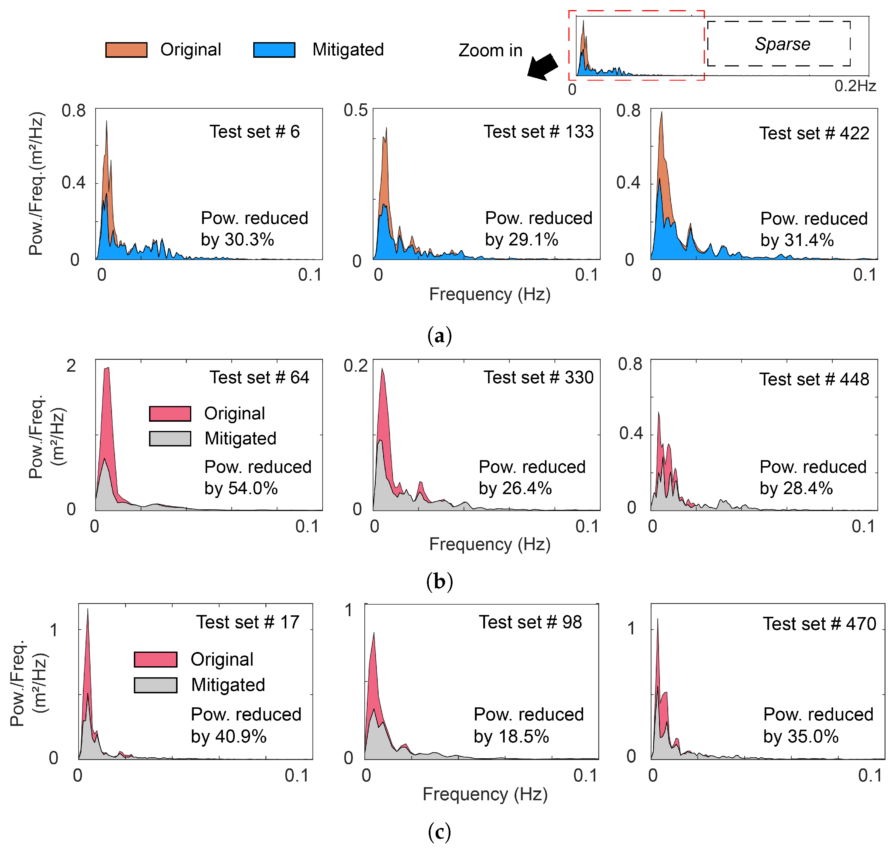
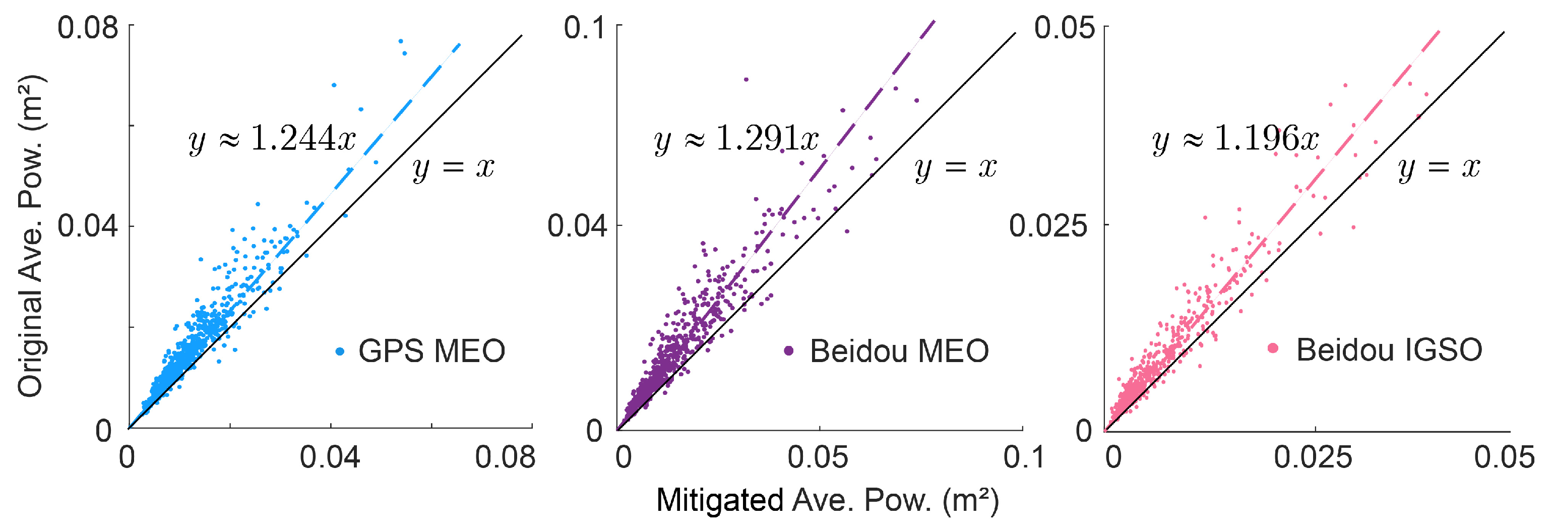
3.2. Power Spectral Density for Mitigated Sequences

The preceding analysis focused on global distribution characteristics through standard deviation metrics, reflecting the network’s temporal predictive performance. Since multipath effects predominantly occupy the low-frequency spectrum, a more precise evaluation examines the network’s performance within this specific band - essentially measuring its multipath mitigation effectiveness. Initial visual assessment utilizes the power spectral density (PSD) of sequences from Figure 9, presented in Figure 11.

This analysis employs linear rather than logarithmic coordinates to better quantify the network’s mitigation capability on an absolute scale. Figure 11 displays PSD comparisons across satellite systems before and after network processing, computed using Welch’s method [44] for power spectrum estimation. Visual inspection reveals consistent power reduction in frequency components associated with multipath effects (higher amplitude regions), with mitigated curves generally positioned below their original counterparts.

$$\mathrm{ASP}={\mathrm{RMS}}^2={\displaystyle \frac{\mathit{1}}{\mathit{N}}}\sum _{\mathit{n}=\mathit{0}}^{\mathit{N}-\mathit{1}}\mathit{x}{\left[\mathit{n}\right]}^{\mathit{2}}$$

(10)

Quantitative analysis appears in Figure 12, presenting comprehensive power suppression statistics across all datasets. The average signal power (ASP), calculated through discrete root-mean-square (RMS) integration (Equation (10)), serves as the primary metric. Total power reduction corresponds to the area difference between original and mitigated regions, representing the network’s interference suppression capability. Specific attenuation levels reach 24.4% for GPS MEO, 29.1% for BeiDou MEO, and 19.6% for BeiDou IGSO - the latter’s lower value reflecting inherently weaker multipath effects compared to MEO satellites.

3.3. Positioning Results

To validate the end-to-end results, we selected data from a certain day (4 April 2023) that not included in the training set to assess the improvement in positioning accuracy. The mitigation ability is limited by the following factors:

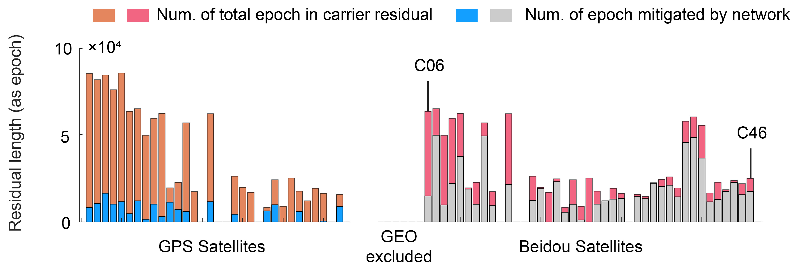
• Due to the network’s stringent requirement for data continuity, only a minor set of the satellite residuals were corrected by the network (as shown in Figure 13). As a result, the improvement in St.D. of the positioning data is less pronounced than that of individual sequences.
• The three-dimensional positioning results underwent sliding mean normalization to align with the dataset’s normalization process (as illustrated in Section 4.3).
• The positioning utilized single-differenced (SD) carrier phase residuals derived from the restoration process (as illustrated in Section 4.1), resulting in a significantly better distribution of solutions compared to using double-differenced (DD) residuals.

The positioning results before and after network correction are plotted in Figure 14. Although the reduction in St.D. is modest, considering that only a small fraction of satellite epochs (as indicated in Figure 13) are involved into dataset, the number of residuals corrected by the network is relatively limited. Nevertheless, the network exhibits clear multipath suppression capability, particularly evident in the mitigation of specific error peaks visible in Figure 14. Enhanced sequence integrity maintenance would likely improve the network’s positioning correction performance.

4. Discussion

4.1. Dataset Preprocessing

Effective preprocessing significantly influences dataset characteristics and consequently, network prediction accuracy. The initial implementation employed DD carrier phase residuals as prediction targets, inadvertently incorporating reference satellite errors. As reference satellite data were absent from the input combinations, this approach yielded suboptimal performance. Building upon Alber’s zero-mean recovery method [45] and its successful application in SD observation extraction [19], we modified the approach to utilize SD residuals between individual satellites and station pairs. As depicted in Figure 3, this implementation requires pseudorange inputs in SD form, with the conversion process mathematically represented in Equation (11).

$$\mathbf{HS}=\left[\begin{array}{ccccc}{w}_1& w_2& w_3& \cdots & w_n\\ 1& -1& 0& \cdots & 0\\ 1& 0& -1& \cdots & 0\\ ⋮& ⋮& ⋮& \ddots & ⋮\\ 1& 0& 0& \cdots & -1\end{array}\right]\left[\begin{array}{c}{s}_{AB}^1\\ s_{AB}^2\\ s_{AB}^3\\ ⋮\\ s_{AB}^n\end{array}\right]=\left[\begin{array}{c}{\displaystyle \sum _{i=1}^n}{w}_i{s}_{AB}^i\\ d_{AB}^{12}\\ d_{AB}^{13}\\ ⋮\\ d_{AB}^{1n}\end{array}\right],\mathrm{with}\sum _{i=1}^n{w}_i{s}_{AB}^i=0$$

(11)

where in Equation (11), $\mathbf{H}$ is the linear combination matrix, $\mathbf{S}$ stands for SD observation vector, ${\omega }_k$ is the weighting factor of satellite k that controlled by elevation $ϵ$ as ${\omega }_k={sin}^2\left(ϵ\right)$. By substituting the obtained DD observations into Equation (11) and applying the zero-mean assumption, one can inversely derive the SD forms of the pseudorange and carrier phase observations, subsequently updating the original dataset.

4.2. Geometry-Based Dataset Segmentation

Construction machinery movement introduces unpredictable multipath interference from the platform. However, the fixed geometric relationship between the platform edge and rover station (illustrated in Figure 6’s lower-left corner) enables unique identification of sea-reflected multipath on the skymap. Satellites positioned within specific elevation and azimuth ranges (marked by light blue shading in Figure 15) consistently experience sea surface reflection multipath effects.

Figure 15 additionally functions as a daily satellite distribution map during the observation period. While environmental obstructions occasionally interrupt satellite trajectories, the receiver antenna generally maintains favorable observation conditions with well-distributed data coverage.

4.3. Data Normalization

Normalization is a crucial step in machine learning tasks, as it allows the network to focus on feature extraction and prediction without being overly concerned with the standard deviation, mean value, and other statistical properties of input data. Unfortunately, in current task, all data magnitudes possess inherent physical significance. To maintain the integrity of mapping function, preprocessing of the dataset’s inputs and outputs is only restricted to the removal of sliding-window moving average (i.e.,compute the moving average sequence over the specified window length, then subtract this moving average sequence from the original sequence). This limitation may constrain the network’s performance, as it must adapt to diverse distribution scenarios, leading to predicted magnitudes that are consistently slightly smaller than the true residuals.

4.4. Network Structures Design

The inspiration for the network architecture stems from the continuous wavelet transform (CWT) method. We treat each channel of the para-TCN as a sampling of the original data, capturing the feature distribution across multiple scales by stacking channels with varying dilation factors, which serve as the scaling factor comparing to wavelets. Consequently, given a specific dilation rate, the data utilized by TCN-backbone can be clearly mapped back to the original signal, as illustrated in Figure 16.

Figure 16 demonstrates how TCN-backbones with varying dilation factors process different segments of the input sequence when kernel size and stride remain fixed. Theoretically, increased utilization of original data within a constrained temporal window enhances the network’s predictive information capacity. However, practical implementation faces computational constraints: excessive TCN-backbone stacking substantially extends training duration. Consequently, the architecture incorporates six parallel pathways with dilation factors $[2, 5, 8, 13, 17, 21]$ as an optimal balance between performance and computational feasibility.

The network’s learning capacity theoretically scales with additional TCN pathways, analogous to the high-resolution feature extraction capability of continuous wavelet transform (CWT). Similar to CWT’s comprehensive signal analysis and reconstruction through inverse CWT (iCWT), additional pathways could potentially improve feature extraction. The current pathway limitation may consequently restrict accuracy by preventing adequate extraction of certain scale (frequency) information due to resolution constraints.

5. Conclusions

The main work of this paper is to mitigate the multipath interference affecting the quality of single-path satellite observations for GNSS antennas that situated near water bodies. In sequential order, it can be primarily summarized into the following points:

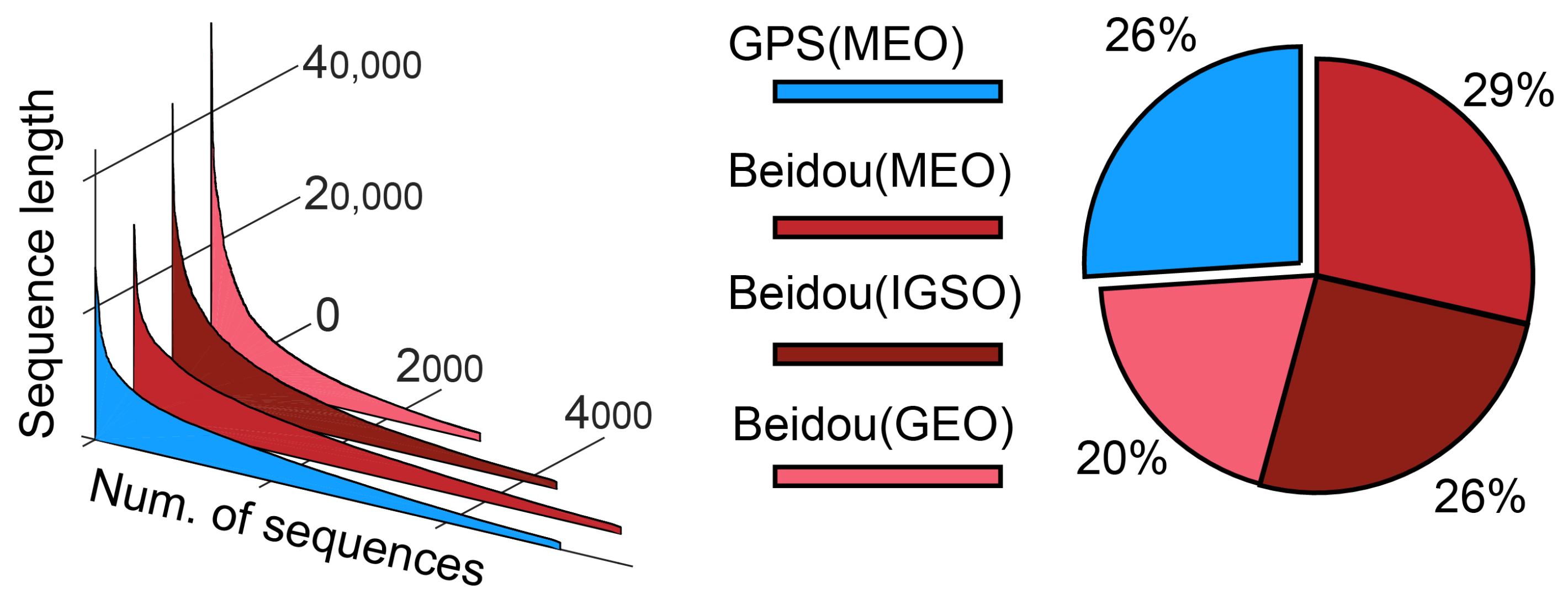
• Comprehensive statistical analysis was performed on GNSS data collected throughout the construction period from maritime platform devices. Theoretical multipath characteristics were derived through geometric analysis, supplemented by shore-based station correction data, resulting in a robust multipath observation dataset (spanning five months, with approximately 93 days of epochs). These datasets have initially demonstrated validity in subsequent network training, and we have reserved the task of delineating air-space maps based on reflection sources for future researchers to conduct more refined studies.
• We identified the primary frequency bands of multipath signals based on the environmental context of this paper. Based on the strong interpretability of the Temporal Convolution Network (TCN), we selected multiple distinct dilation factors to construct a multi-channel parallel para-TCN network for real-time prediction of multipath effects. Since our input data are all collected before RTK processing, it could avoid the influence of real-time processing errors on the network’s performance. The datasets utilized are geometrically independent observations, while networks extracts the real-time variations in multipath caused by structural dynamic displacements through small-dilation TCN backbones and captures the frequency continuity of multipath effects in the low-frequency range through large-dilation backbones, thus holding potential for structural dynamic monitoring.
• Validation employed a 90%/10% dataset split. Results demonstrate residual standard deviation suppression between 12.4% and 14.3%, with average signal power reduction ranging from 19.6% to 29%. Post-processing distribution improvements were observed in nearly all cases, with minimal instances of degradation, confirming the network’s robustness and accurate multipath characteristic identification capability.

Future research directions focus on acquiring more extensive and stable datasets to enhance network training and predictive performance through refined training methodologies. While the current work establishes a foundational framework for real-time multipath processing, several areas require development: network architecture scalability remains unexplored, and predictive accuracy shows potential for significant improvement. Although input data types and network architectures may undergo substantial evolution, the core methodology of multipath component extraction from observation data by deep learning method represents a promising direction for carrier multipath mitigation.

References

1. Meng, X.; Xi, R.; Xie, Y. Dynamic characteristic of the forth road bridge estimated with GeoSHM. J. Glob. Position. Syst. 2018, 16, 4. [Google Scholar] [CrossRef]
2. Wang, J.; Meng, X.; Qin, C.; Yi, J. Vibration Frequencies Extraction of the Forth Road Bridge Using High Sampling GPS Data. Shock Vib. 2015, 2016, 1–18. [Google Scholar] [CrossRef]
3. Xi, R.; Chen, H.; Meng, X.; Jiang, W.; Chen, Q. Reliable Dynamic Monitoring of Bridges with Integrated GPS and BeiDou. J. Surv. Eng. 2018, 144, 04018008. [Google Scholar] [CrossRef]
4. Xi, R.; Jiang, W.; Meng, X.; Chen, H.; Chen, Q. Bridge monitoring using BDS-RTK and GPS-RTK techniques. Measurement 2018, 120, 128–139. [Google Scholar] [CrossRef]
5. Niu, Y.; Xiong, C. Analysis of the dynamic characteristics of a suspension bridge based on RTK-GNSS measurement combining EEMD and wavelet packet technique. Meas. Sci. Technol. 2018, 29, 085103. [Google Scholar] [CrossRef]
6. Yi, T.H.; Li, H.N.; Gu, M. Experimental assessment of high-rate GPS receivers for deformation monitoring of bridge. Measurement 2013, 46, 420–432. [Google Scholar] [CrossRef]
7. Yang, A.; Wang, P.; Yang, H. Bridge Dynamic Displacement Monitoring Using Adaptive Data Fusion of GNSS and Accelerometer Measurements. IEEE Sens. J. 2021, 21, 24359–24370. [Google Scholar] [CrossRef]
8. Kaloop, M.; Li, H. Multi input–single output models identification of tower bridge movements using GPS monitoring system. Measurement 2014, 47, 531–539. [Google Scholar] [CrossRef]
9. Han, H.; Wang, J.; Meng, X.; Liu, H. Analysis of the dynamic response of a long span bridge using GPS/accelerometer/anemometer under typhoon loading. Eng. Struct. 2016, 122, 238–250. [Google Scholar] [CrossRef]
10. Cawley, P.; Adams, R. The Location of Defects in Structures from Measurements of Natural Frequencies. J. Strain Anal. Eng. Des. 1979, 14, 49–57. [Google Scholar] [CrossRef]
11. Ge, L.; Han, S.; Rizos, C. GPS multipath change detection in permanent GPS stations. Surv. Rev. 2002, 36, 306–322. [Google Scholar] [CrossRef]
12. Xi, R.; Xu, D.; Jiang, W.; He, Q.; Zhou, X.; Chen, Q.; Fan, X. Elimination of GNSS carrier phase diffraction error using an obstruction adaptive elevation masks determination method in a harsh observing environment. GPS Solut. 2023, 27, 139. [Google Scholar] [CrossRef]
13. Wang, S.Y. Detection and Analysis of GNSS Multipath. 2016; pp. 1–3. Available online: https://www.diva-portal.org/smash/get/diva2:937141/FULLTEXT02.pdf (accessed on 2 February 2025).
14. Kanhere, A.V.; Gupta, S.; Shetty, A.; Gao, G. Improving GNSS Positioning Using Neural-Network-Based Corrections. Navig. J. Inst. Navig. 2022, 69, navi.548. [Google Scholar] [CrossRef]
15. Pugliano, G.; Robustelli, U.; Rossi, F.; Santamaria, R. A new method for specular and diffuse pseudorange multipath error extraction using wavelet analysis. GPS Solut. 2016, 20, 499–508. [Google Scholar] [CrossRef]
16. Delgado, N.; Haag, M. Multipath analysis using code-minus-carrier for dynamic testing of GNSS receivers. In Proceedings of the 2011 International Conference on Localization and GNSS (ICL-GNSS), Tampere, Finland, 29–30 June 2011. [Google Scholar] [CrossRef]
17. Dong, D.; Wang, M.; Chen, W.; Zeng, Z.; Song, L.; Zhang, Q.; Cai, M.; Cheng, Y.; Lv, J. Mitigation of multipath effect in GNSS short baseline positioning by the multipath hemispherical map. J. Geod. 2015, 90, 255–262. [Google Scholar] [CrossRef]
18. Fuhrmann, T.; Luo, X.; Knöpfler, A.; Mayer, M. Generating statistically robust multipath stacking maps using congruent cells. GPS Solut. 2014, 19, 83–92. [Google Scholar] [CrossRef]
19. Zhong, P.; Ding, X.; Yuan, L.; Xu, Y.; Kwok, K.; Chen, Y. Sidereal filtering based on single differences for mitigating GPS multipath effects on short baselines. J. Geod. 2009, 84, 145–158. [Google Scholar] [CrossRef]
20. Atkins, C.; Ziebart, M. Effectiveness of observation-domain sidereal filtering for GPS precise point positioning. GPS Solut. 2015, 20, 111–122. [Google Scholar] [CrossRef]
21. Gao, R.; Liu, Z.; Odolinski, R.; Jing, Q.; Zhang, J.; Zhang, H.; Zhang, B. Hong Kong–Zhuhai–Macao Bridge deformation monitoring using PPP-RTK with multipath correction method. GPS Solut. 2023, 27, 195. [Google Scholar] [CrossRef]
22. Chang, G.; Chao, C.; Yang, Y.; Xu, T. Tikhonov Regularization Based Modeling and Sidereal Filtering Mitigation of GNSS Multipath Errors. Remote Sens. 2018, 2018, 1801. [Google Scholar] [CrossRef]
23. Zhang, Z.; Guo, F.; Zhang, X.; Pan, L. First result of GNSS-R-based sea level retrieval with CMC and its combination with the SNR method. GPS Solut. 2022, 26, 20. [Google Scholar] [CrossRef]
24. Larson, K.; Löfgren, J.; Haas, R. Coastal sea level measurements using a single geodetic GPS receiver. Adv. Space Res. 2013, 51, 1301–1310. [Google Scholar] [CrossRef]
25. Wang, X.; He, X.; Zhang, Q. Evaluation and combination of quad-constellation multi-GNSS multipath reflectometry applied to sea level retrieval. Remote Sens. Environ. 2019, 231, 111229. [Google Scholar] [CrossRef]
26. Roussel, N.; Ramillien, G.; Frappart, F.; Darrozes, J.; Biancale, R.; Striebig, N.; Hanquiez, V.; Bertin, X.; Allain, D.J. Sea level monitoring and sea state estimate using a single geodetic receiver. Remote Sens. Environ. 2015, 171, 261–277. [Google Scholar] [CrossRef]
27. Zhang, Z.; Li, B.; Gao, Y.; Shen, Y. Real-time carrier phase multipath detection based on dual-frequency C/N0 data. GPS Solut. 2018, 23, 7. [Google Scholar] [CrossRef]
28. Wang, N.; Xu, T.; Gao, F.; Xu, G. Sea Level Estimation Based on GNSS Dual-Frequency Carrier Phase Linear Combinations and SNR. Remote Sens. 2018, 10, 470. [Google Scholar] [CrossRef]
29. Gao, W.; Meng, X.; Gao, C.; Pan, S.; Zhu, Z.; Xia, Y. Analysis of the carrier-phase multipath in GNSS triple-frequency observation combinations. Adv. Space Res. 2018, 63, 2735–2744. [Google Scholar] [CrossRef]
30. Reichert, A.K. Correction Algorithms for GPS Carrier-Phase Multipath Utilizing the Signal-to-Noise Ratio and Spatial Correlation. Master’s Thesis, University of Colorado, Boulder, CO, USA, 1999; pp. 23–24. [Google Scholar]
31. Bilich, A.; Larson, K. Mapping the GPS multipath environment using the signal-to-noise ratio (SNR) (vol 42, art no RS6003, 2008). Radio Sci. 2007, 43, RS3839. [Google Scholar] [CrossRef]
32. Hofmann-Wellenhof, B.; Lichtenegger, H.I.M.; Wasle, E. GNSS-Global Navigation Satellite Systems: GPS, GLONASS, Galileo, and More; Springer: Vienna, Austria, 2007; pp. 154–158. [Google Scholar]
33. Teunissen, P.J.G.; Kleusberg, A. GPS for Geodesy; Springer: Berlin/Heidelberg, Germany, 1998; pp. 176–182. [Google Scholar] [CrossRef]
34. Bidikar, B.; Chapa, B.P.; Kumar, M.V.; Rao, G.S. GPS Signal Multipath Error Mitigation Technique. In Satellites Missions and Technologies for Geosciences; Demyanov, V., Becedas, J., Eds.; IntechOpen: Rijeka, Croatia, 2020; Chapter 4. [Google Scholar] [CrossRef]
35. Krypiak-Gregorczyk, A.; Wielgosz, P. Carrier phase bias estimation of geometry-free linear combination of GNSS signals for ionospheric TEC modeling. GPS Solut. 2018, 22, 45. [Google Scholar] [CrossRef]
36. Bolla, P.; Won, J.H. Performance Analysis of geometry-free and ionosphere-free code-carrier phase observation models in integer ambiguity resolution. IET Radar Sonar Navig. 2018, 12, 1313–1319. [Google Scholar] [CrossRef]
37. Jiang, Y.; Wang, J. Extracting relevant patterns from GNSS observations to mitigate multipath in RTK deformation monitoring. GPS Solut. 2024, 28, 200. [Google Scholar] [CrossRef]
38. Wang, Y.; Zhao, W.; Shen, Y.; Yu, S. Research on multipath suppression performance of multiple BOC signals of navigation satellite. IOP Conf. Ser. Mater. Sci. Eng. 2020, 793, 012044. [Google Scholar] [CrossRef]
39. Vaswani, A.; Shazeer, N.M.; Parmar, N.; Uszkoreit, J.; Jones, L.; Gomez, A.N.; Kaiser, L.; Polosukhin, I. Attention is All you Need. In Proceedings of the Neural Information Processing Systems, Long Beach, CA, USA, 4–9 December 2017. [Google Scholar] [CrossRef]
40. Brown, T.B.; Mann, B.; Ryder, N.; Subbiah, M.; Kaplan, J.; Dhariwal, P.; Neelakantan, A.; Shyam, P.; Sastry, G.; Askell, A.; et al. Language Models are Few-Shot Learners. arXiv 2020, arXiv:2005.14165. [Google Scholar] [CrossRef]
41. Bai, S.; Kolter, J.; Koltun, V. An Empirical Evaluation of Generic Convolutional and Recurrent Networks for Sequence Modeling. arXiv 2018, arXiv:1803.01271. [Google Scholar] [CrossRef]
42. Jin, F.; Zhang, K.; Huang, Y.; Zhu, Y.; Chen, B. Parallel Spatio-Temporal Attention-Based TCN for Multivariate Time Series Prediction. Neural Comput. Appl. 2022, 35, 13109–13118. [Google Scholar]
43. Yang, Z.; Zhang, Y.; Qian, K.; Wu, C. SLNet: A Spectrogram Learning Neural Network for blackDeep Wireless Sensing. In Proceedings of the 20th USENIX Symposium on Networked Systems Design and Implementation (NSDI 23), Boston, WA, USA, 17–19 April 2023. [Google Scholar]
44. Welch, P. The use of fast Fourier transform for the estimation of power spectra: A method based on time averaging over short, modified periodograms. IEEE Trans. Audio Electroacoust. 1967, 15, 70–73. [Google Scholar] [CrossRef]
45. Alber, C.; Ware, R.; Rocken, C.; Braun, J. Obtaining Single Path Delays from GPS Double Differences. Geophys. Res. Lett. 2000, 27, 2661–2664. [Google Scholar] [CrossRef]
Figure 1. Geometry of an off-shore based GNSS antenna infected by possible multipath signals.
Remotesensing 17 00601 g001
Figure 2. Phase diagram of a multipath infected signal.
Remotesensing 17 00601 g002
Figure 3. The flowchart illustrating how trained network support the positioning process. GNSS observation would experience regular RTK resolution once to obtain current residuals to feed into networks, then those predicted multipath would serve as the correction to help mitigate multipath in current carrier phase residuals.
Remotesensing 17 00601 g003
Figure 4. Diagram of dataset construction, data processing and network training. Noted that the para-TCN sets are bunch of network identity in structure yet differed by the input dataset which utilized in network training. Here P.R. is short for pseudorange, Res. for residual, and C.P. for carrier phase. Geometric (near-field environment) segmentation is optional as marked with asterisk, and specific details can be found in Section 4.
Remotesensing 17 00601 g004
Figure 5. On the left displays a statistical representation the properties of collected data, with each horizontal axis representing a sequence and the vertical axis indicating its length, providing further insight into the concentration of GEO and IGSO satellite data. The right figure illustrates the comparison of total data volume for the corresponding categories.
Remotesensing 17 00601 g005
Figure 6. Detailed characterization of the offshore construction platform (multipath data acquisition site) and near-field environments of the GNSS base and rover stations. The platform’s pile foundation is anchored into bedrock, ensuring structural rigidity. The rover antenna is situated in a tidal zone where sea level fluctuations induce dynamic sea surface reflections. A functional relationship between satellite elevation and azimuth angles within sea surface reflection regions can be derived based on geometric constraints.
Remotesensing 17 00601 g006
Figure 7. The CWT diagram of the code multipath effect, wherein h = 10 m and a constant reflection coefficient α = 0.01 . The fundamental frequency of the multipath effect initiates at 0.029 Hz and decreases with an increasing elevation angle. Concurrently, the third harmonic component vanishes at medium elevation angles, while the second harmonic component disappears at high elevation angles.
Remotesensing 17 00601 g007
Figure 8. Network framework using parametric TCNs, where the input consists of observations and code multipath, while the output is a real-time prediction sequence for multipath signals. The detail of colored blocks could be referring to the right corner.
Remotesensing 17 00601 g008
Figure 9. The network’s suppression effect of sequence distribution of (a) a calculation example of local St.D. of carrier residual before and after mitigation (b) GPS MEO cases (c) Beidou MEO cases (d) Beidou IGSO case. The order of each sequence within the entire test set is indicated in the upper-left corner of the subplots, and the rate of distribution change is recorded above each plot.
Remotesensing 17 00601 g009aRemotesensing 17 00601 g009b
Figure 10. The St.D. of the residual sequences before and after mitigation: All dataset. Each point in the graph represents St.D. of a case before (y-axis) and after (x-axis) mitigation, while the dashed line represents their linear fit. Therefore, the line slope indicates the percentage expectation of data correction achieved by the network.
Remotesensing 17 00601 g010
Figure 11. Power spectral density (PSD) of residual sequences before and after mitigation for (a) GPS MEO (b) Beidou MEO (c) Beidou IGSO satellites, while Pow. and Freq. are short for Power and Frequency, respectively. Data presents in the figure are identity with those of Figure 9. As illustrated on the topside, each PSD has been locally enlarged for better visualization. Additionally, owing to variations in data distribution, the coordinate scales differ across the figures.
Remotesensing 17 00601 g011
Figure 12. A comparison of the average signal power across all datasets before and after mitigation, presented in a format consistent with Figure 10. As a statistical representation of Figure 11, the network demonstrates a significant ability to suppress the frequency bands affected by multipath (in quadratic form, the dominant frequencies become more pronounced).
Remotesensing 17 00601 g012
Figure 13. The number of observed epochs for all satellites recorded on 1 April 2023, and the proportion of these epochs that were corrected by the network.
Remotesensing 17 00601 g013
Figure 14. The ENU (East-North-Up) three-dimensional displacement for part of the data before and after network processing. The network’s suppression effect on data distribution is partially reflected in the mitigation of periodic component peaks.
Remotesensing 17 00601 g014
Figure 15. Skymap of the GNSS rover antenna. Area within the light blue shadowed area is the region affected by sea reflection, as shown in lower-left corner of Figure 6.
Remotesensing 17 00601 g015
Figure 16. Diagram of the TCN-backbone architecture, using simplified parameters to represent the original sequence nodes utilized in computing the value of a single node in the output layer. Three input layers below contain identical input data, with color variations used to distinguish between different dilation rates.
Remotesensing 17 00601 g016