Modelling LiDAR-Based Vegetation Geometry for Computational Fluid Dynamics Heat Transfer Models

Abstract

Vegetation characteristics significantly influence the impact of wildfires on individual building structures, and these effects can be systematically analyzed using heat transfer modelling software. Close-range light detection and ranging (LiDAR) data obtained from uncrewed aerial systems (UASs) capture detailed vegetation morphology; however, the integration of dense vegetation and merged canopies into three-dimensional (3D) models for fire modelling software poses significant challenges. This study proposes a method for integrating the UAS–LiDAR-derived geometric features of vegetation components—such as bark, wooden core, and foliage—into heat transfer models. The data were collected from the natural woodland surrounding an elevated building in Samford, Queensland, Australia. Aboveground biomass (AGB) was estimated for 21 trees utilizing three 3D tree reconstruction tools, with validation against biomass allometric equations (BAEs) derived from field measurements. The most accurate reconstruction tool produced a tree mesh utilized for modelling vegetation geometry. A proof of concept was established with Eucalyptus siderophloia, incorporating vegetation data into heat transfer models. This non-destructive framework leverages available technologies to create reliable 3D tree reconstructions of complex vegetation in wildland–urban interfaces (WUIs). It facilitates realistic wildfire risk assessments by providing accurate heat flux estimations, which are critical for evaluating building safety during fire events, while addressing the limitations associated with direct measurements.

1. Introduction

Fires that originate in wildland vegetation (wildfires, forest fires, or bushfires) cause extensive devastation around the world each year, particularly when they interact with concentrations of human settlement [1,2]. Wildfires are often difficult to control, especially when they spread rapidly through tree crowns [3]. Catastrophic wildfires often occur where urban edges are surrounded by wildland, which places numerous buildings adjacent to flammable vegetation [4]. Fire in these areas, variously known as the wildland–urban interface (WUI) [5], urban–bushland interface [6], residential–wildland interface [7], and peri-urban area [8], can rapidly transition between natural and man-made sources of fuel [1]. Human population in WUIs has been growing rapidly in recent years as people choose a ‘tree-change’ lifestyle [9]. It is therefore increasingly essential to understand the wildfire risk at these interfaces, so that preventative measures can be implemented and safety improved. However, the complex interplay of risk factors is not well understood and can be difficult to assess [1].

Remote sensing technologies, including satellites, uncrewed aerial systems (UASs), and crewed aircraft [5], have been used in recent wildfire studies to collect spectral [10] and structural information from wildlands, enabling risk to be assessed non-destructively [11,12,13]. UAS surveys deliver the highest spatial resolution data at a low cost and high level of safety, with a trade-off of lower spatial coverage [14]. However, as WUIs are often confined to small areas of land [2], UASs are ideally suited to collecting comprehensive WUI data that capture the proximity of vegetation to residential structures and allow a better assessment of risk than historical data alone [15].

LiDAR scans using UASs are particularly suitable for collecting high-resolution structural data at close range compared to alternative methods [14]. This combination captures essential measures, including building location and design elements, structural vegetation characteristics, and topographic slopes, resulting in a complete point cloud representation of the surveyed area. This high-density point cloud enables the structural geometry and topology of vegetation to be accurately reconstructed [16]. Point clouds are now frequently used to reconstruct trees and other vegetation, aided by advances in computing capability and procedural modelling algorithms [17]. These advances have superseded earlier methods of vegetation modelling that were based on rules and repeating patterns [17]. Tree reconstruction with procedural modelling algorithms is a multi-step process, which involves the creation of a three-dimensional (3D) triangulated mesh from a 3D point cloud. The mesh is created by first constructing a tree skeleton, which depicts the trunk and main branch structures as an ensemble of straight or tapering cylinders [18]. Branch surfaces are then geometrically reconstructed and added to the skeleton [19]. Cylindrical geometry is used because it produces robust and reliable quantitative structural models (QSMs) and highly accurate estimates of dimensions such as length, diameter, angle, orientation, and volume [19,20,21].

Information from LiDAR point clouds can also be organized into a structured grid of equivolume 3D units known as voxels, in which each voxel has an assigned position [22]. Voxelized point clouds are emerging as a high-potential source of 3D fuel information in fire simulations. For example, Marcozzi et al. [23] voxelized a point cloud collected with a terrestrial laser scanner in a laboratory setting, in which the point cloud was segmented into ‘branch wood’ and ‘foliage’ classes. Voxels inherit the attributes of the points they encompass, thus encoding rich information that is more informative than estimates of spatial volume based on a coordinates grid [22].

Several studies have utilized fire dynamics simulation software to investigate vegetation fire using a numerical modelling approach in a 3D simulation environment [3,24,25,26,27]. The Fire Dynamics Simulator (FDS) is a simulation tool developed at the National Institute of Standards and Technology (NIST) that incorporates physics-based fire models [28]. Physics-based models are used to generate heat transfer estimates from fuel property information [29]. The WUI Fire Dynamics Simulator (WFDS) is an extended version of the FDS, which incorporates the spread of fire in vegetative fuels and is thus appropriate for modelling wildfires. For example, Mell et al. [25] simulated grassland fire in the WFDS with a simple fuel model that predicted fire spread behaviour, which was consistent with empirical observations. However, the FDS is sometimes considered to simulate complex fire environments more fully, as it can incorporate a greater number of features [26]. Ganteaume et al. [26] demonstrated the functional adequacy of the FDS by accurately depicting WUI fire behaviour based on historical fire incidents. Hendawitharana et al. [30] used the FDS to incorporate complex features and architectural design elements with high dimensional accuracy. They combined airborne and ground-based LiDAR point clouds to obtain a 3D model of a building. They incorporated the model into a grass fire simulation to examine the risk in relation to wind velocity, temperature, and pressure.

However, wildfires are not restricted to ground-level grass fires. They can also appear as elevated crown fires, which are generally caused by surface fires that propagate along the bark of tree trunks, or through direct contact between flames and branches that are adorned with foliage [3]. Despite the importance of fuel type distribution in crown fire spread [31], 3D reconstructions of tree structure are generally omitted from WUI fire simulations [5]. Rather, geometric shapes that simplify complex vegetation structures are used. For example, laboratory experiments were conducted by Mell et al. [24] and Moinuddin et al. [3] to test a numerical model using the WFDS that is capable of estimating the spatial distribution of vegetation within a tree crown. For simplicity, Douglas fir (Pseudotsuga menziesii) was used for these studies, whereby the vegetation was assumed to be uniformly distributed within a tree crown that exhibited a clearly defined geometric shape. Such simplification imposes homogeneity on the crown structure and therefore on the assumed fuel distribution. In reality, crown structure is often heterogeneous, particularly in natural forests [32]. Imposed homogeneity can undermine the accuracy of fire spread simulations, as heterogeneous crown structure responds differentially to fire intensity, in terms of time to ignition, magnitude, and dynamic spread [23,33]. Remote sensing offers the capability to extract important structural information and address this omission. In particular, LiDAR-informed estimates of fuel distribution have been shown to increase the accuracy of dynamic fire simulations. The high-resolution data provide fine-scale information that is particularly important when canopy is heterogeneous [23].

Fire simulations are often based on computational fluid dynamics (CFD), which is currently the most advanced means of representing fire behaviour at the sub-stand scale (less than 1 km) [29]. Solid fuel sources in CFD models are generally assigned simple geometries and thermal properties [34]. In reality, these elements are often complex. The inclusion of more detailed structural information would allow CFD models to more accurately predict the interactions that influence wildfire behaviour [35]. However, integrating complex fuel geometries into CFD models remains challenging [17]. CFD models in the FDS require two primary elements to be defined: obstructive objects (OBSTs) and Lagrangian particles (PARTs). PARTs represent various types of vegetation that are smaller than the numerical modelling grid, such as leaves and grass [28,34]. PARTs are treated as static sources of heat absorption and emission that contribute to airflow obstruction and are subject to thermal degradation [26]. Modelling these solid fuel sources as collections of sub-grid particles allows irregular shapes and varying thermal properties to be represented, which allows for the spatial distribution of heat release to be modelled [34]. Gaps that occur between fuel particles can also play an important role in ignition [23].

Moreover, the 3D structure provides important information on the characteristics and spatial distribution of different types of fire fuel, but is currently overlooked in most WUI fire simulations [5]. However, reconstructed 3D meshes are surface representations that depict branches as cylinders with triangular faces, outlining the boundaries of the branches with hollow interiors, whereas OBSTs and PARTs in the FDS require solid shapes to be defined as rectangular, axis-aligned forms, which are characterized by specifying two points. Therefore, to allow reconstructed tree geometry to be accurately represented in the FDS environment, we describe a method for populating the reconstructed mesh with voxel grids.

The purpose of this work is to propose a methodology for integrating the 3D structure of vegetation into the FDS environment, including coniferous to deciduous species, utilizing UAS–LiDAR remote sensing. Three tree reconstruction algorithms—Raycloudtools, AdTree, and TreeQSM—were compared using UAS–LiDAR data and ground truth measurements to identify the most suitable method for the integration. This study expands on the work of Hendawitharana et al. [30] by incorporating the detailed structure of vegetation surrounding an elevated house in a WUI. Specifically, our objective is to produce a geometric representation of three distinct vegetation elements, namely bark, wooden core, and foliage, so that the unique combustion characteristics of each element can be incorporated into the FDS. We first merged UAS–LiDAR and handheld LiDAR point clouds of the area surrounding the building. We then segmented individual trees and produced reconstructions of the vegetation structure with three different reconstruction algorithms, which we evaluated with a biomass allometric equation (BAE). Finally, we used the best-performing tree reconstruction algorithm to generate a geometrical representation of the vegetation and its components for use in the FDS simulation environment.

2. Materials and Methods

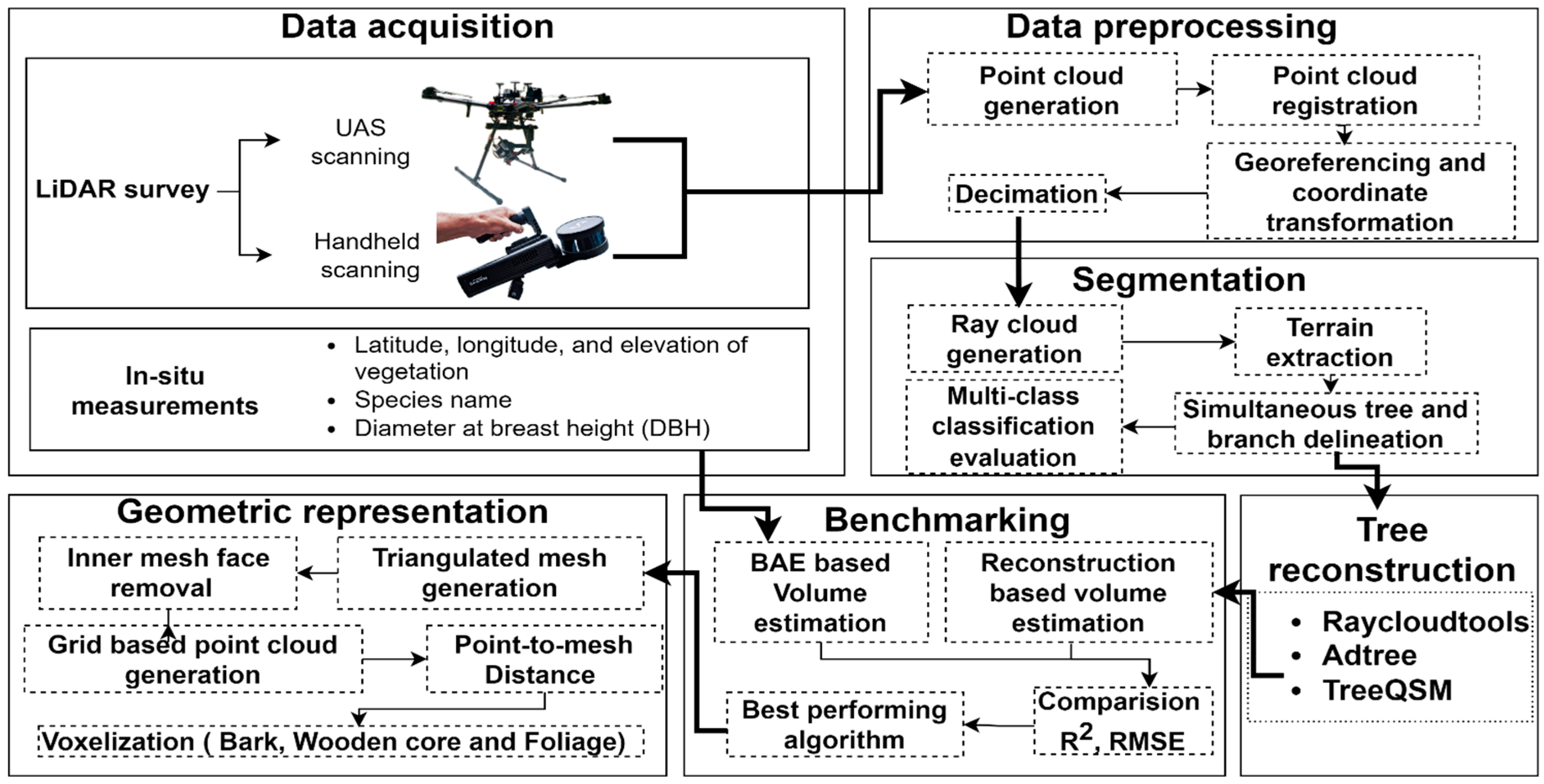
2.1. Process Pipeline

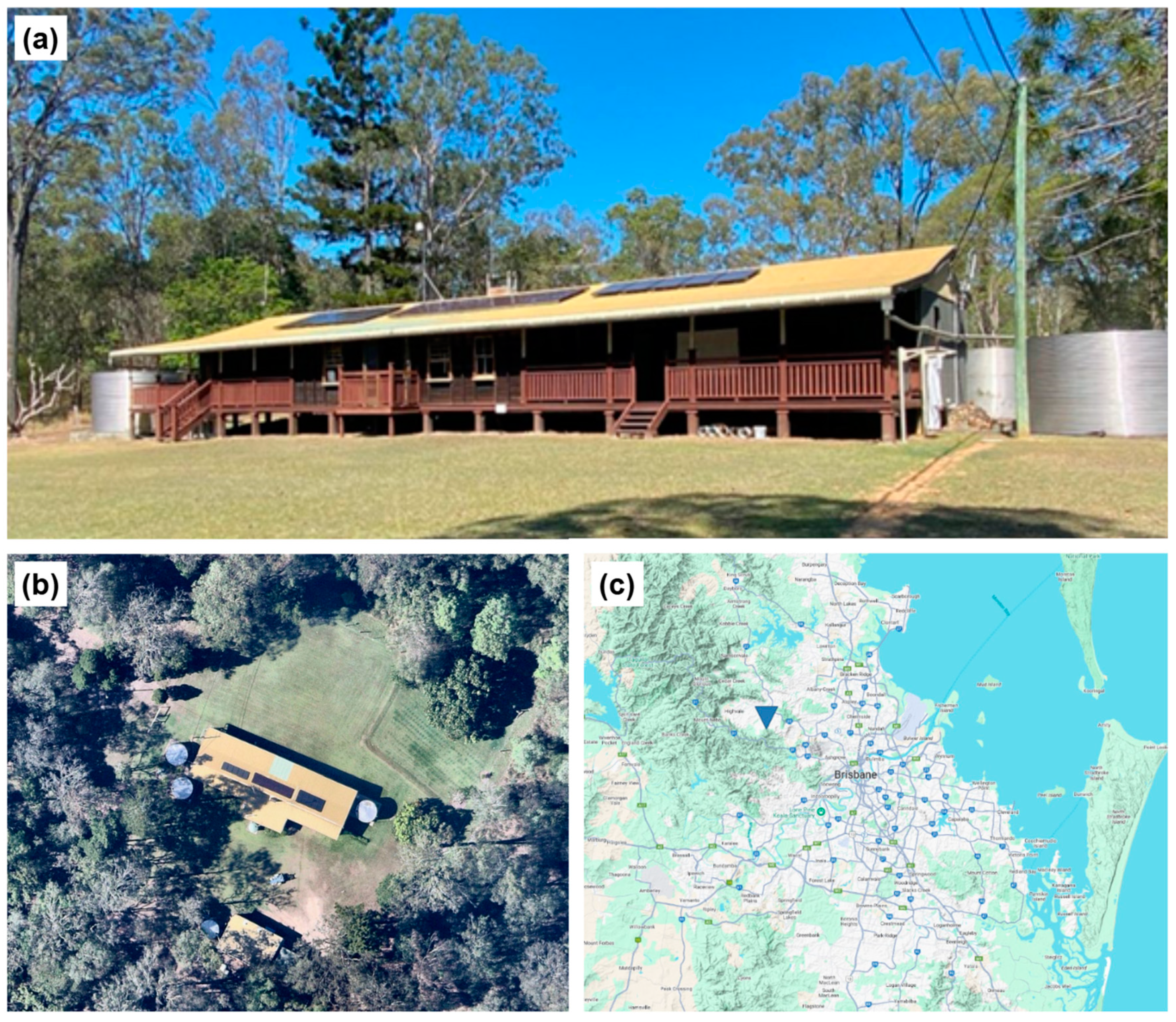
The process pipeline, as shown in Figure 1, consisted of a series of six core components: data acquisition, preprocessing, segmentation, tree reconstruction, benchmarking, and geometric representation.

Surveys were carried out using both UAS–LiDAR and handheld LiDAR systems around the chosen building. Point clouds were generated and preprocessed to ensure registration within a consistent coordinate system prior to merging. Subsequently, individual trees were segmented from the merged point cloud and three state-of-the-art 3D reconstruction algorithms were applied. A benchmarking study was conducted using the BAE-derived volume estimation to compare the results of the three 3D tree reconstruction algorithms. Finally, the geometric representation of the vegetation, composed of bark, wooden core, and foliage components, was derived from the benchmarked reconstructed tree mesh in the form of voxels.

2.2. Study Site

We selected an elevated building in a WUI located in Samford, Queensland, Australia (Figure 2), with overall dimensions of 30 m × 10 m × 4.85 m. Elevated buildings are common in Queensland, but their response to bushfires is still unknown.

Vegetation had been cleared on three sides of the building, from between 8 m and 30 m away from the structure, and the rest of the land was surrounded by several species of vegetation [30]. Due to all the above factors, the selected building is highly vulnerable during wildfires, which makes it ideal for the proposed study.

2.3. LiDAR Data Acquisition

Data collection from the surrounding environment was multi-modal, employing active remote sensing methods, as well as field surveys. Active sensing using LiDAR sensors, both UAS-mounted and handheld, enabled the capture of surrounding structural and spectral information from the air and in the field. LiDAR data were collected from the air and the ground with a Hovermap ST LiDAR system (developed by Emesent, headquartered in Brisbane, Australia) on 15 February 2023. The system consisted of 16 LiDAR channels and +/−20 mm mapping accuracy, with a sensing range of 0.4 m to 100 m. The airborne survey was conducted using a real-time kinematic (RTK) DJI M300RTK UAS system (developed by DJI, headquartered in Shenzhen, China) flown at 50 m altitude in a double lawn mower pattern (perpendicular grids), with a flight line spacing of 50 m and a wind speed threshold of 10 kmh⁻¹. Figure 3 shows the survey path and point cloud acquired from the (a) handheld and (b) UAS surveys. The two point clouds were preprocessed, then merged using Emesent Aura software tools (version 1.5; Emesent Pty Ltd., Milton, Australia, 2021) following the methodology outlined in the study of Hendawitharana et al. [30]. The merging resulted in a final point cloud of approximately 12 GB in size, with a very high density of approximately 450 points/m².

2.4. Field Measurements and Ground-Based Observations

A ground truth survey of vegetation attributes within 40 m of the building was conducted two weeks after the UAS scan. The survey followed a secure route through the dense vegetation. Ground-based LiDAR data were collected utilizing the Hovermap ST in handheld mode. In situ data were collected for all large trees (>10 cm diameter at breast height (DBH), approximately 1.3 m above ground) close to the building, including species identification, DBH, and age, and latitude, longitude, and elevation were measured at each tree location with an Emlid Reach RS2+ (developed by Emlid, headquartered in Budapest, Hungary) RTK global navigation satellite system (GNSS) receiver. Twenty-one large trees were identified on which our tree reconstruction would be based. Eleven different species were represented, of varying size and geometry. The species, field-measured DBH, and field-measured height of these trees are provided in

Table 1. Field measurements of the 21 large trees closest to the building.

No	Name	DBH (cm)	Height (m)
1	Plumeria pudica	6.4	3.3
2	Lophostemon suaveolens	13.0	8.0
3	Macadamia integrifolia	14.6	12.6
4	Jagera pseudorhus	18.0	9.6
5	Melaleuca salicina	20.8	11.0
6	Lophostemon suaveolens	20.0	12.6
7	Corymbia intermedia	21.0	16.5
8	Corymbia intermedia	22.6	14.6
9	Callitris columellaris	20.0	18.5
10	Lophostemon suaveolens	48.0	25.8
11	Melaleuca salicina	25.2	13.8
12	Corymbia tessellaris	22.1	19.6
13	Lophostemon suaveolens	26.9	18.3
14	Corymbia intermedia	34.6	20.3
15	Callitris columellaris	35.0	21.0
16	Callitris columellaris	37.6	20.1
17	Eucalyptus siderophloia	34.8	25.7
18	Corymbia tessellaris	48.0	25.9
19	Araucaria bidwillii	55.4	22.4
20	Eucalyptus siderophloia	58.0	29.2
21	Lophostemon confertus	84.0	21.6

.

Figure 4 provides images of the (a) remote sensing survey equipment (UAS and handheld LiDAR) and (b) in situ data collection.

2.5. Tree Segmentation with Raycloudtools

Tree segmentation was performed with command-line tools in Raycloudtools. A ray cloud file was first created by combining the LiDAR point cloud with the UAS trajectory data. Ray clouds differ from point clouds in that they contain information on empty spaces (air) within the cloud, in addition to the surface geometry, which allows volumetric analyses to be undertaken [36]. The ray cloud was then spatially decimated using the ‘raydecimate’ tool, to one point per 3 cubic cm, and a 50 cm threshold was applied to eliminate rays with isolated endpoints. A ground mesh was extracted with the ‘rayextract:terrain’ tool. Non-vegetation regions, including the building, were segmented out (removed) from the ray cloud in the area closest to the building. The remaining ray cloud and the ground mesh (representing terrain data) were then fed into the ‘rayextract:trees’ tool, which simultaneously delineated all tree and branch structures, resulting in 21 individual trees being automatically segmented.

2.6. Evaluation of Raycloudtools Segmentation

UAS–LiDAR remote sensing is an effective tool for vegetation mapping [37], but it becomes challenging in regions with high plant diversity and overlapping canopies [38]. Thus, the performance of the ray cloud tool was evaluated against manually segmented point clouds. Ray clouds in Raycloudtools are stored in the Stanford PoLYgon (.ply) format, which is compatible with point cloud processing programmes such as CloudCompare [36]. This allowed us to validate the performance of the automated Raycloudtools segmentation, from which the tree reconstructions would be generated in the following step. We loaded the cloud produced in the previous step, with the non-vegetation regions (including the building) removed, into CloudCompare (v2.12.4 (Kyiv)). We then manually identified and segmented the same 21 trees that were automatically segmented by Raycloudtools. We first used the Colorimetric Segmenter (Filter RGB option) to filter all points associated with each individual tree from the point cloud, then the Segment Out tool (Polygon Out option) to remove points that represented surrounding vegetation and noise, based on visual assessment. The manually segmented trees were then used as benchmarks to assess the accuracy of the automated Raycloudtools segmentation, in which the 21 manually segmented trees were considered to represent 21 different classes. The assessment was carried out following the multi-class classification evaluation approach outlined by Rauch et al. [39]. The process involved comparing the class assigned to each point in the automatically segmented trees with its corresponding reference (manually segmented) class. A confusion matrix was then derived that allowed us to compute precision, recall, and F1-score values based on four fundamental measures: true positive (TP), true negative (TN), false negative (FN), and false positive (FP). TP refers to the number of segmented points that were correctly assigned to a particular class, TN refers to the number of correct non-classified points, FN refers to the number of non-classified points that should have been assigned to a particular class, and FP refers to the number of segmented points that were incorrectly assigned to a particular class. In multi-class scenarios, FP, FN, and TN cannot be obtained directly from the confusion matrix (as they can in the binary case). In these scenarios, the metrics must be calculated separately for each class based on the summation scheme [39]. The equations used to derive the evaluation metrics are provided in

Table 2. Evaluation metrics.

Metrics	Equation	Remarks
Accuracy	${\displaystyle \frac{TP+TN}{TP+TN+FP+FN}}$	Accuracy of a classification increases with correctly segmented points that belong to a particular class
Precision	${\displaystyle \frac{TP }{TP+FP}}$	Precision decreases with the number of incorrectly segmented points that are included in a particular class
Recall	${\displaystyle \frac{TP }{TP+FN}}$	Recall decreases the number of incorrectly segmented points that should be assigned to a particular class but are not
F1-score	${\displaystyle \frac{2\times Precision\times Recall}{Precision+Recall}}$	F1-score is a weighted harmonic mean of precision and recall

.

2.7. Tree Reconstruction

A comprehensive evaluation was then conducted of three different open-source tree reconstruction tools (AdTree [16], TreeQSM [19,40], and Raycloudtools [36]). These tools are commonly used to reconstruct tree models from laser-scanned (LiDAR) point clouds with demonstrated accuracy ([16,36,41]) and represent an evolution in tree reconstruction algorithms. Each tool employs a different approach for producing the initial tree skeletons, which form the basis of the 3D triangulated meshes. AdTree uses a minimum spanning tree (MST) algorithm to identify the main branch points and initialize the skeleton, then simplifies the structure by eliminating small edges and redundant vertices that have minimal impact. TreeQSM was designed to improve and extend the AdTree method [41]. TreeQSM uses a region growing method to generate the tree skeleton from subsets of the point cloud, called cover sets, which are treated as patches in the vegetation surface. Raycloudtools first segments the points into subgraphs and the neighbouring points are connected. The subgraphs contain a root node often at the tree’s base, which serves as the starting point for skeleton creation. Dijkstra’s shortest path algorithm is applied to create a disjoint acyclic graph from the root node. Subgraphs representing additional branches of the tree are then added to the primary skeleton. This extension involves a bidirectional probing process to identify connecting points. AdTree and Raycloudtools use allometric models to fit the shorter branches, because point noise that occurs near branch tips makes cylinder fitting difficult. The allometric models in this context estimate the relative growth of a particular branch in comparison to a standard.

Table 3. Summary of tree reconstruction algorithms.

Algorithm	Skeleton Generation	Trunk Fitting	Branch Fitting
AdTree	Minimum spanning tree (MST) using Dijkstra’s shortest path algorithm	Cylinder fitting	Allometric models
TreeQSM	Region growing method with segmented point cloud (cover sets)	Cylinder fitting
Raycloudtools	Disjoint acyclic graph using Dijkstra’s shortest path algorithm from root nodes	Cylinder fitting	Allometric models

provides a summary of the methods employed by the tools.

2.8. Reconstructed Branch Volume Comparison

The accuracy of each reconstruction was benchmarked by comparing the tree mesh volume estimates with the BAE-derived estimates of stem wood volume. Using the structural details of the cylinders, the total tree branch volume was calculated for each tool by combining the volumes of all the cylinders that made up each branch and the main stem, according to the fundamentals of calculating cylindrical volumes.

The BAE shown in Equation (1) was used to calculate oven dry above-ground biomass (AGB) in a non-destructive manner, using the field measurements collected from the 21 trees closest to the building in our study area:

M = 0.0673 × (ρD²H)^0.976

(1)

where M = oven dry AGB (kg), ρ = Stem-specific density (gcm⁻³), D = DBH (cm), and H = total tree height (m) [42]. The stem-specific density is a parameter calculated by dividing the oven dry mass of a section of a plant’s main stem by the volume of the corresponding fresh section. This BAE was designed to calculate the oven dry AGB of pantropical trees incorporating trunk, branch, and foliage biomass. However, the foliage biomass was neglected in our comparison, as the foliage to woody structure ratio of the vegetation was low [43]. The oven dry AGB estimates were then divided by the density values to arrive at the final estimates of wood volume (V) (Equation (2)).

V = M/ρ

(2)

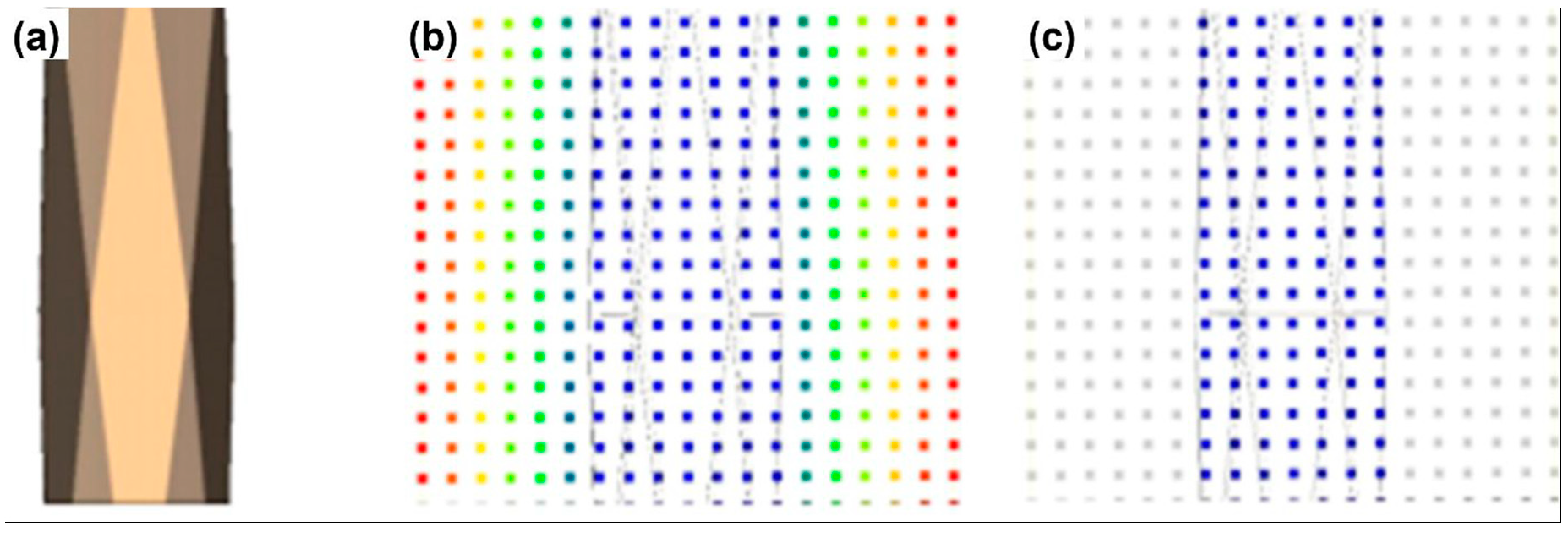
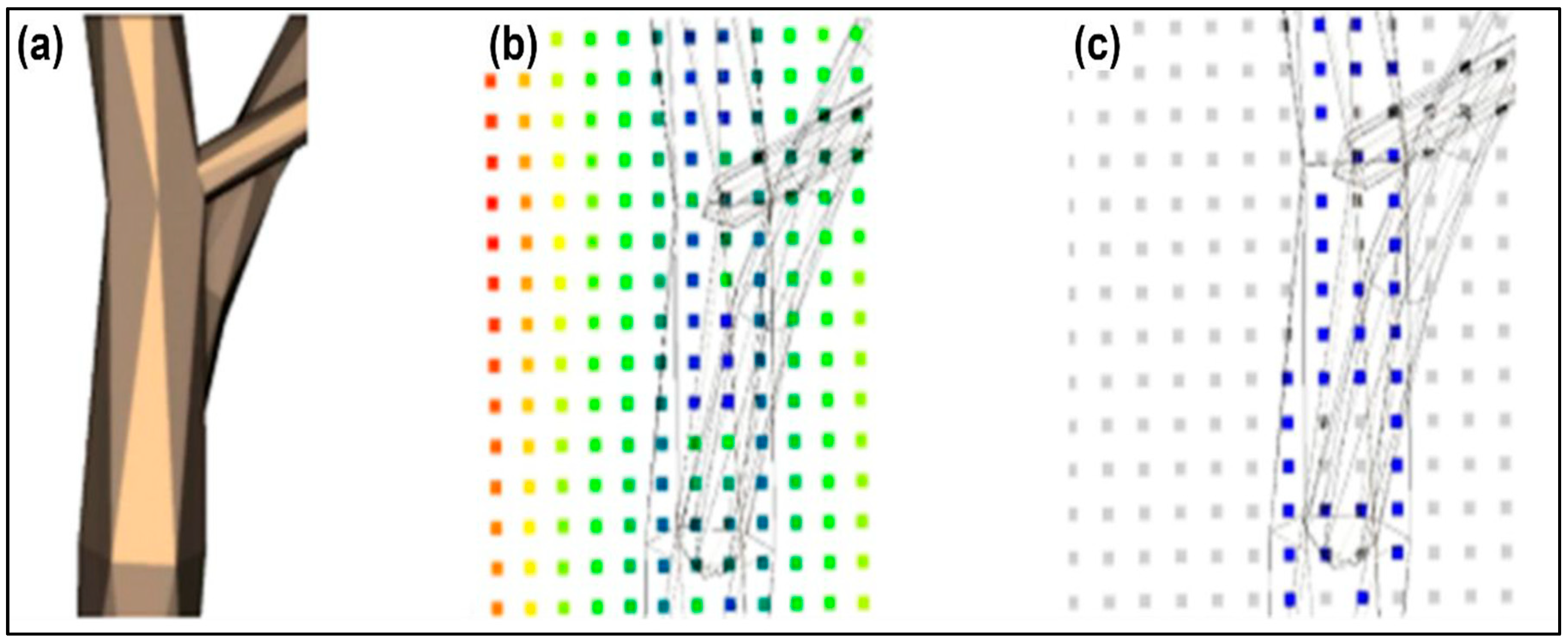
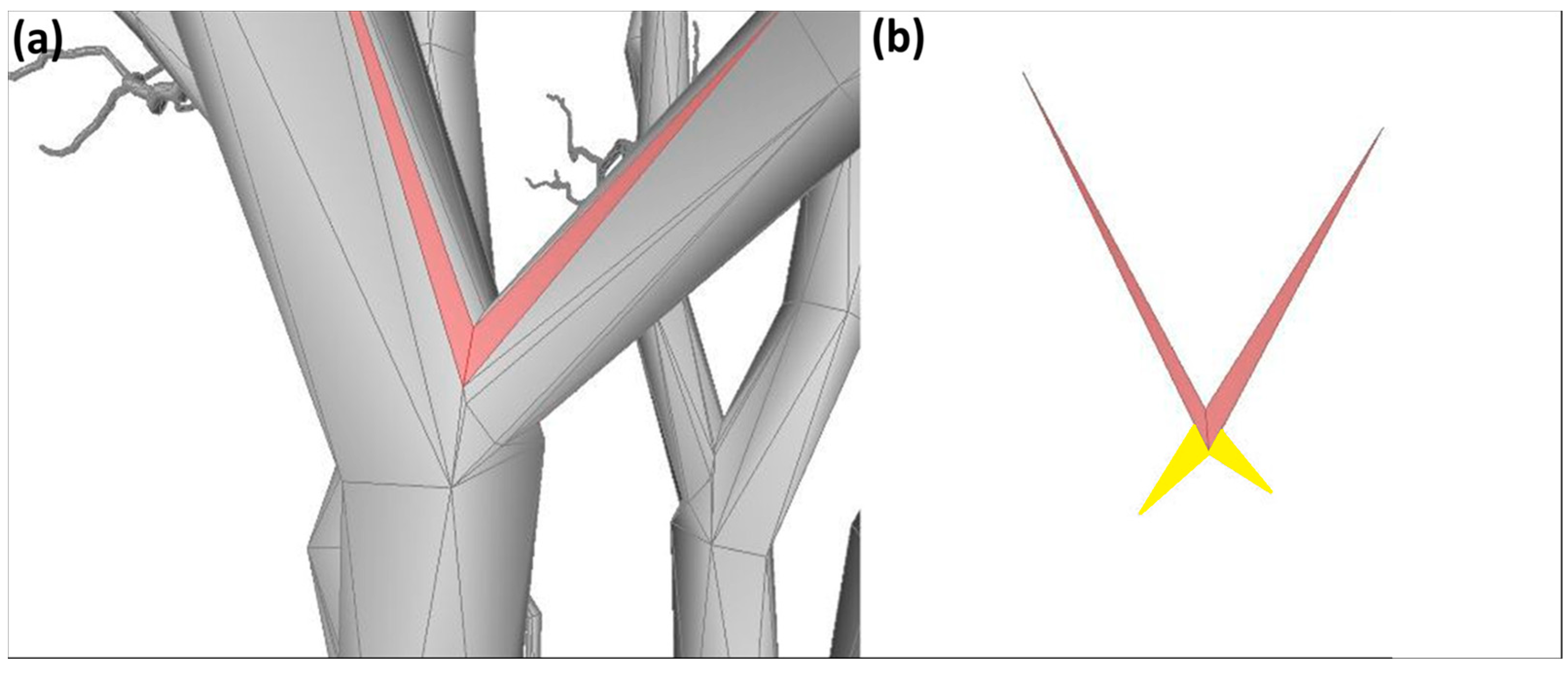
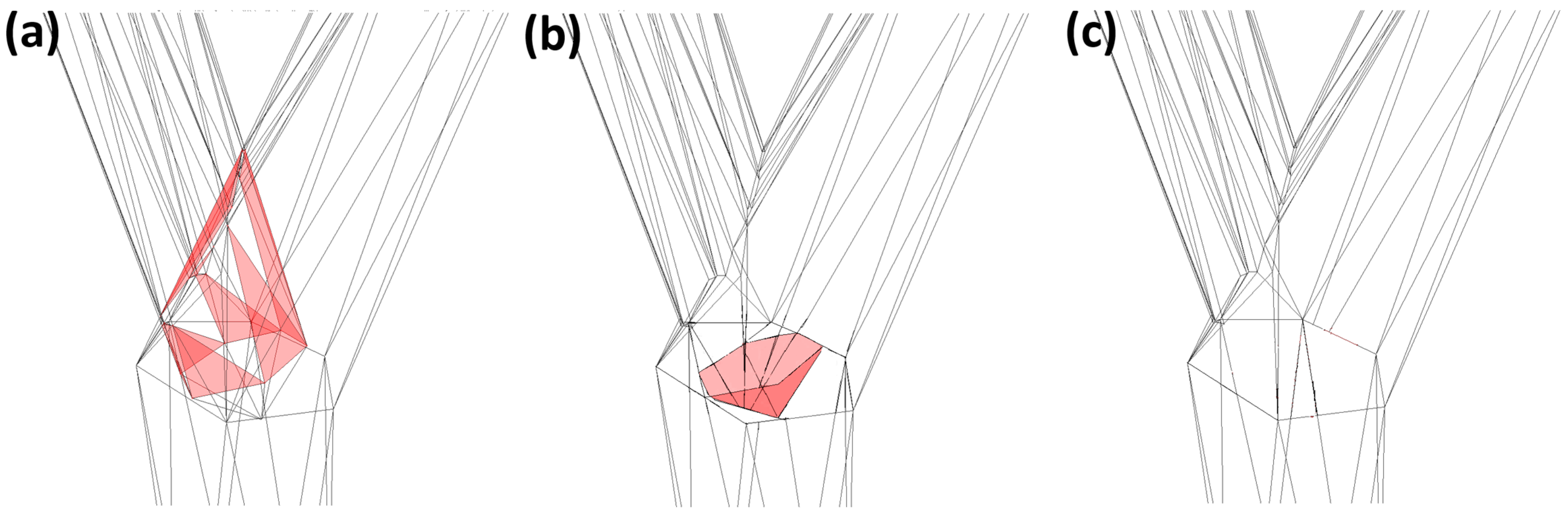
2.9. Geometric Representation of Vegetation

We used the best-performing tool (highest accuracy compared with BAE-derived estimates) to create a geometric representation of the solid fuel sources (bark, wooden core, and foliage) of a single tree in our study site. The aim was to produce an accurate particle model from the triangulated 3D mesh (Figure 5a) that would be suitable for use in the FDS. The faces in the mesh were oriented with the normal vector pointing away from the cylinder axis. We first created a grid-based point cloud within the smallest rectangular bounding box that could accommodate the reconstructed tree mesh at a resolution of 10 cm, based on the grid used by Mell et al. [24] for 5 m tall trees. We filtered out points that fell outside the mesh and calculated the distance from each remaining point to the nearest face (Figure 5b). We then voxelized the tree stem based on the points that occurred within the negative orientation of the normal vector (Figure 5c).

In this study, the mesh to point cloud distances were computed using CloudCompare (version 2.12.4) [GPL software]. The nearest point to the mesh, whether located on the positive or negative side of the face, represents the outer layer of the stem, specifically the geometry of the bark.

However, the reconstructed mesh does not only encompass the outer surface of the tree. The cylindrical representations of tree skeletons resulted in intersecting cylinders and intersecting faces at junctions where a parent branch had more than one child branch (Figure 6a). Points in the grid-based point cloud that were located within the parent branch and near the intersecting face (Figure 6b) were assigned distances with a positive orientation from the face. Without removing the inner faces, these voxels would have been excluded from the stem (Figure 6c).

For the purpose of removing inner faces from the reconstructed mesh, we employed a segmentation process whereby intersecting faces were partitioned along the intersecting line. Initially, curvature flipping optimization was conducted using the MeshLab tool (Version, 2022.02) [44] to eliminate folded faces during the reconstruction process. Then, using the Blender software (Version, 3.6) [45], these intersecting faces were partitioned and triangulated. This resulted in a series of non-manifold vertices, where each plane was divided into an inner face and outer face, with the normal vector oriented away from the corresponding cylinder axis, producing a set of four interconnected faces (Figure 7).

We employed a systematic approach to removing the two inner faces from each non-manifold edge, to leave only the outer faces in the reconstructed tree mesh. We initially organized the faces into pairs, with each pair comprising one inner face and one outer face (f1, f2 and f3, f4) characterized by the same normal vector direction (Figure 8).

A single face was then selected from each pair, and a critical vector, denoted V, was computed using Equation (3):

V = V_t − V_m

(3)

where V_m signifies the position vector located at the midpoint of the two vertices connecting the non-manifold edge, while V_t represents the position vector associated with the third vertex, which is not connected to the non-manifold edge. Following this calculation, the dot product between V_t and the normal vector of the plane formed by the remaining pair of faces was evaluated. This dot product serves as the pivotal criterion for identifying whether the selected face is an inner or outer face. A positive dot product value indicates that the chosen face is an outer face, with the other face in the pair designated as the inner face. Conversely, a negative dot product value signifies that the chosen face is the inner face, while the counterpart is identified as the outer face.

Once all the inner faces of the non-manifold edges were eliminated, the internal meshes became detached from the outer mesh. Subsequently, faces with border edges that were not connected with more than one face were identified and progressively removed until none remained. Subsequently, the outermost layer of the geometric representation was extracted, consisting of the points closest to the mesh, which were identified as the vegetation’s bark, while the remaining points were designated as part of the wooden core. Voxelization of the foliage was achieved by isolating the point cloud located within a 20 cm distance (the width of 2 voxels) of the reconstructed mesh from the segmented vegetation point cloud. The remaining points space was divided into cubic grid volumes, with a resolution of 10 cm. These volumes containing points were labelled as foliage voxels. The finalization of the voxelization process resulted in an accurate 3D representation of the tree geometry that can be used within the FDS environment to quantify the spatial distribution of sub-grid solid fuel sources.

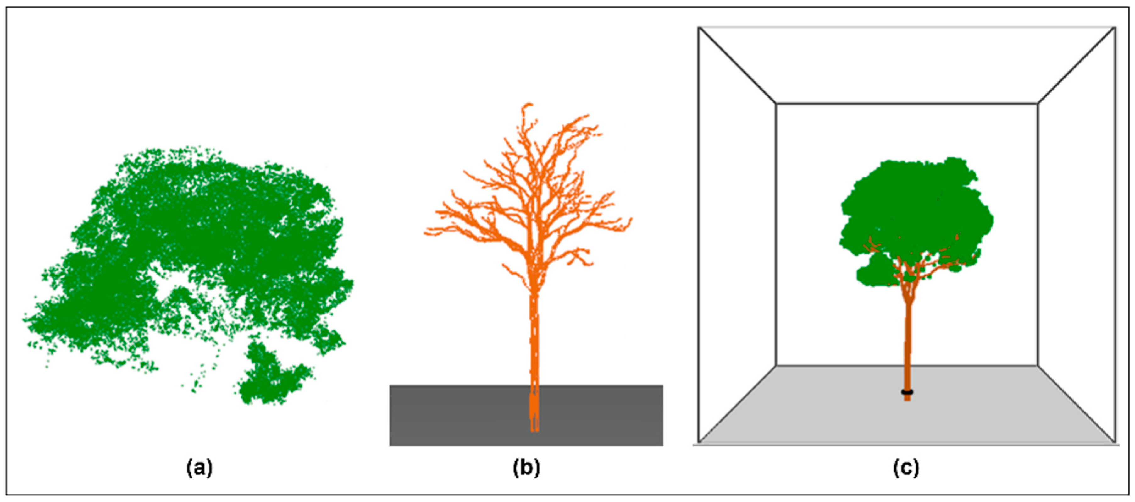
2.10. Proof of Concept

The methodology we have presented for quantifying the combustible components of a reconstructed tree produces information that is suitable for incorporation into FDS models. This method was influenced by previous research, notably the Douglas fir tree modelling [24], which produced reasonable simulations from experiments and suggested that detailed modelling of non-combustible parts, like the wooden core, is not essential. In fact, many researchers, including Wickramasinghe et al. [46], have represented the wooden core as a cylindrical solid element, which is treated as inert material. It has also been noted that typically, only the bark and the small, thick branches of trees are consumed in bushfires. In particular, the Douglas fir tree experiments revealed that branches smaller than 6 mm tend to burn in controlled laboratory settings [24].

Based on these insights, we used our geometric representation of a Eucalyptus siderophloia to undertake a proof of concept in which we considered only the bark and foliage components as combustible parts. We assigned the bark voxels to OBSTs, with an auxiliary text file created following FDS guidelines. We voxelized the foliage as described above, then designated a single particle in each voxel that encapsulated the combustible fuel content and assigned thermo-physical properties of that voxel. This approach aligned with the techniques used in the Douglas fir tree particle model [24]. However, our method diverged in the specifics of the voxel/grid definition. Unlike the Douglas fir tree model, where the cone geometry inherent in the FDS facilitates automatic particle placement in voxels to represent foliage, the structural characteristics of Australian tree species necessitated a different strategy. This is due to the variance in foliage geometry from the standard cone or cylinder geometry available in the FDS. To accommodate this important difference, our proof of concept involved the creation of an auxiliary text file, following PART specifications. This auxiliary file allows the spatial information from the voxelized point cloud to inform the spatial distribution of Lagrangian particles in the FDS model. We expect that this approach will produce a spatially explicit, heterogenous canopy that represents the distinct foliage geometry of Australian trees more accurately than the simplified geometries.

3. Results

3.1. Tree Segmentation

Figure 9 shows the output of the automated Raycloudtools segmentation, representing the 21 field-measured trees closest to the building, and the results of the manual segmentation of the same individual point clouds in CloudCompare. Based on the 21 classes represented in the manual CloudCompare segmentation (one class for each tree), the automated segmentation using Raycloudtools achieved an average accuracy of 98%, with 90% precision, 87% recall, and an F1-Score of 87%. Despite some confusion with merging canopy areas, adequate spacing between trunks enabled accurate segmentation of individual trees.

3.2. Comparison of Field Measurements and Reconstructed Tree DBH

The comparison between field measurements and reconstructed tree DBH using Adtree, TreeQSM, and Raycloudtools is summarized in

Table 4. Comparison of Reconstructed Tree Diameters with Field Measurements (RMSE—Root Mean Square Error, R²—Coefficient of Correlation).

Reconstruction Algorithm	RMSE	R2
Adtree	55.50	0.73
TreeQSM	17.58	0.89
Raycloudtools	13.54	0.95

. The table presents the root mean square error (RMSE) and the coefficient of correlation (R²) for each method. The RMSE reflects the average magnitude of error, while the correlation coefficient indicates the strength of the relationship between reconstructed diameters and field measurements.

3.3. Reconstructed Branch Volume Comparison

In addition to field-measured heights and DBH, stem-specific density values were required for BAE-based volume estimation. We obtained values for nine of the eleven species from the Global Wood Density Database [47,48]. We note that the value for Callitris columellaris was given as wood density, which was equivalent to stem-specific density in other species. We applied a stem-specific density value of 0.7 gcm⁻³ to Macadamia integrifolia and Plumeria pudica, for which measurements could not be found, calculated as the mean of the nine obtained values (

Table 5. Density values obtained for field-measured tree species (* = no data found).

Species	Common Name/s	Number in Field Sample	Wood Density (g·cm−3)	Stem-Specific Density (g·cm−3)
Araucaria bidwillii	Bunya pine	1	0.39–0.46 (mean 0.42)	0.42
Callitris columellaris	Sandy/white cypress pine	3	0.58	*
Corymbia intermedia	Pink bloodwood	3	*	0.8
Corymbia tessellaris	Moreton Bay ash	2	0.90–0.93 (mean 0.92)	0.91
Eucalyptus siderophloia	Grey ironbark	2	0.95	0.95
Jagera pseudorhus	Foambark	1	0.68	0.68
Lophostemon confertus	Brush box	1	0.72–0.76 (mean 0.75)	0.75
Lophostemon suaveolens	Swamp box	4	0.55–0.76 (mean 0.69)	0.73
Macadamia integrifolia	Macadamia nut	1	*	*
Melaleuca salicina (Callistemon salignus)	Willow/white-flowering bottle brush	2	0.84	0.84
Plumeria pudica	Frangipani	1	*	*

).

The BAE-based volume estimates were compared with the volumes of the tree reconstructions produced by each of the three tools (Figure 10). Root mean square errors (RMSE) and coefficients of correlation (R²) were calculated to evaluate the performance of each tool (

Table 6. Performance comparison with BAE-based volume estimation (RMSE—Root Mean Square Error, R²—Coefficient of Correlation).

Reconstruction Algorithm	AdTree	TreeQSM	Raycloudtools
R2	0.525	0.908	0.972
RMSE (m3)	500.94	20.30	0.85

). The Raycloudtools volume estimation achieved a higher R² (0.972 vs. 0.525 and 0.908) and a RMSE two orders of magnitude lower than AdTree and TreeQSM (8.5 × 10⁻¹ vs. 5 × 10² and 2 × 10¹).

3.4. Geometric Representation of Vegetation

A Eucalyptus siderophloia (tree #20: height = 29.2 m, DBH = 58.0 cm) was selected for the voxelization process, in which we produced a geometric representation suitable for input into the FDS environment. Figure 11 shows the segmented point cloud and Figure 12 shows the reconstructed mesh of the tree produced by each of the three tools. Based on its superior performance, Raycloudtools was selected for our proof of concept.

Where cylinders intersected within the mesh, which is a surface representation, we used a dot product-based indicator to differentiate the inner faces from the outer faces, so that the inner faces could be discarded (Figure 13). We then identified and removed the border faces from cylinder intersections (Figure 14) to produce the final mesh. Figure 15 shows a section of the completed voxelization in which the final mesh was successfully populated with the point cloud grid.

A comparative analysis of the voxelization technique before and after the removal of the internal sections of intersecting cylinders demonstrated that after the internal sections were removed, the voxelization incorporated all the points that fell inside the reconstructed tree.

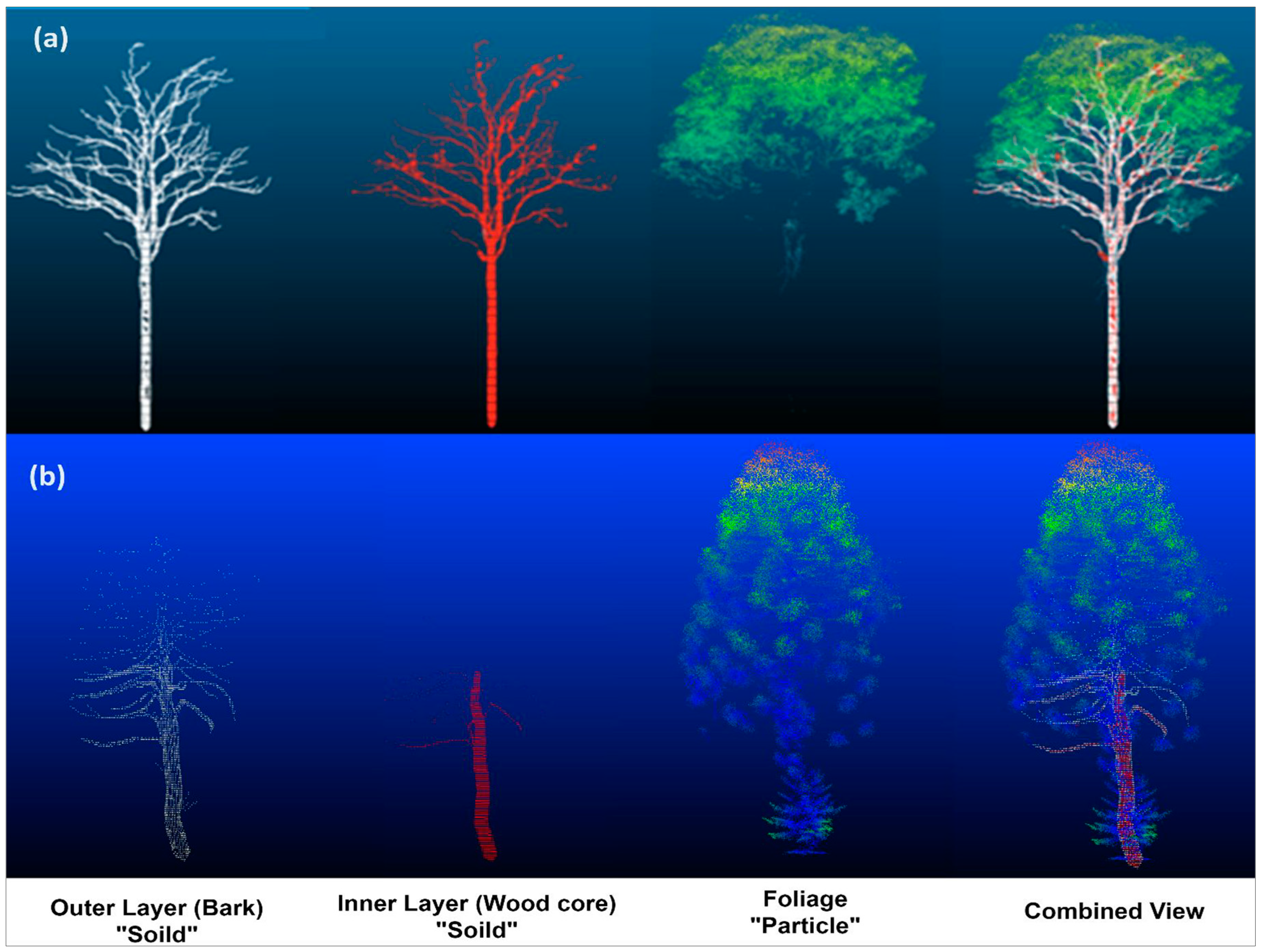
3.5. Classification of Fuel Components

Wooden core and bark classification was based on the proximity of points to the final mesh that we reconstructed from the voxelized point cloud grid. Foliage points were obtained by filtering the points closest to the mesh reconstructed from the LiDAR point cloud. This removed the points associated with the main branches. Points associated with branches less than 2 cm thick were then considered as foliage points. In the reconstruction of tree crowns, we considered only the main branches contributing to the tree skeleton. Figure 16 shows the results of this classification process for a Eucalyptus siderophloia (deciduous tree) and Araucaria bidwillii (coniferous tree), in which points were designated as wooden core, bark, or foliage.

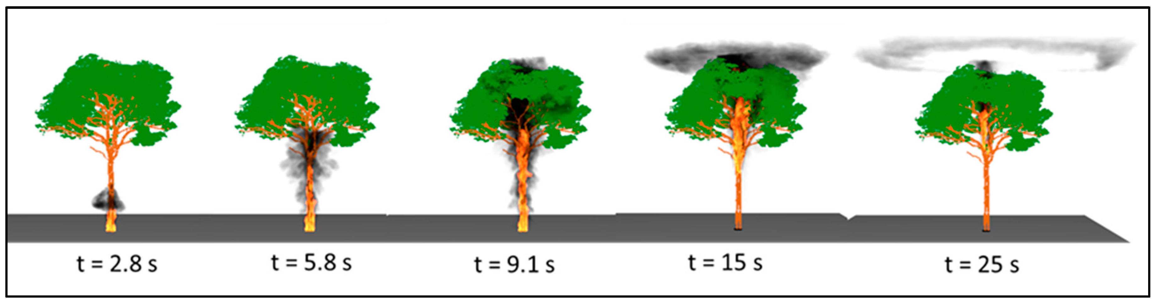
3.6. Fire Simulation of Eucalyptus Siderophloia

The auxiliary text files detailing the foliage particles and the main branches were integrated into an FDS model using Fortran code. Figure 17 provides an illustration of the FDS model, depicting both the foliage and wooden core as well as presenting a comprehensive view of the FDS model tailored to Eucalyptus siderophloia.

The initiation of ground fire was simulated through the use of ignitor particles. Subsequent to the ignition of the ground fuel, the advancement of the fire was monitored. Figure 18 depicts the successful propagation of the fire from the stem to the canopy.

4. Discussion

This study aimed to develop a methodology to create a geometric representation of three distinct vegetation elements—bark, wooden core, and foliage—by incorporating their unique combustion characteristics into FDS models. This was achieved through a comprehensive approach, integrating data acquisition (via LiDAR surveys and in situ measurements), point cloud segmentation, tree reconstruction with advanced tools such as Raycloudtools, AdTree, and TreeQSM, and the geometric representation of vegetation elements. The results demonstrate significant progress in integrating UAS–LiDAR data into 3D tree reconstructions and heat transfer modelling.

In this study, Raycloudtools demonstrated exceptional performance in instance segmentation tasks, achieving an average accuracy of 98%, with a precision of 90%, recall of 87%, and an F1-score of 87%. These results highlight the effectiveness of the method, particularly in a WUI area, which is characterized by lower vegetation density and fewer overlapping vegetation structures. This performance aligns with the findings of Cherlet et al. [49], who benchmarked various instance segmentation methods and identified Raycloudtools as the best-performing tool. In their study, it successfully detected approximately 70% of trees in a dense forest plot with 50% precision, even under challenging conditions such as overlapping crowns, dense vegetation, and variable growth patterns. The significantly higher accuracy achieved in this study, particularly in the WUI context, suggests that RayCloudTools is well suited to environments with reduced vegetation density where segmentation challenges are comparatively less pronounced.

The comparative analysis of reconstructed tree diameters against field measurements demonstrated varying levels of accuracy and reliability among the reconstruction tools. Raycloudtools outperformed AdTree and TreeQSM, achieving the highest coefficient of correlation (R² = 0.95) and the lowest RMSE, indicating superior alignment with ground truth data. TreeQSM followed, with an R² of 0.89, while AdTree exhibited the poorest performance, with an R² of 0.73 and the highest RMSE. Similarly, Raycloudtools outperformed AdTree and TreeQSM in vegetation volume estimation, achieving an R² of 0.972 and an RMSE of 0.85 m³, compared to R² values of 0.525 and 0.908 for AdTree and TreeQSM, respectively.

A critical factor influencing the performance of tree reconstruction algorithms is their ability to handle low-density point clouds, which commonly arise in natural environments due to noise and penetration limitations, particularly when trunks are obscured by foliage [50]. AdTree relies on merging adjacent vertices, which can deprioritize sparse regions, while TreeQSM’s region-growing algorithm encounters difficulties in forming cover sets in areas with a low point density. However, Raycloudtools effectively addresses these limitations by incorporating all points into a disjoint acyclic graph, enabling more accurate branch representations. In the final step of reconstruction, AdTree and Raycloudtools use allometric models to fit cylinders for other branches based on the length and radius of the parent branch. TreeQSM, on the other hand, does not use allometric models for branch tips, which might explain its poor performance. The TreeQSM algorithm assumes that the vegetation point cloud adequately covers the tree at a low noise level. However, the movement of foliage in the wind causes points to become noisier as they move through the branches. Morhart et al. [51] used QSMs and concluded that volume estimates may not be reliable in actual forest environments where environmental factors can further degrade data quality. Similarly, Lau et al. [52] evaluated the performance of TreeQSM in reconstructing the architecture of tropical trees and found that the method tended to overestimate the lengths and volumes of smaller branches. The results indicate that Raycloudtools exhibits significant advantages in natural environments, particularly under conditions of noise and wind-induced movement that exacerbate low-density point cloud challenges, enabling more accurate tree reconstruction. While this approach may be challenged if multiple layers of trees with dense foliage overlap [53], such as in tropical forests, it appears to be a reliable and user-friendly solution for individual tree segmentation in areas where vegetation is less dense, such as WUIs. An example of the different outputs of each algorithm, based on the 3D mesh reconstructions of a Callitris columellaris, is provided in Figure 19.

Finally, the voxelization methodology proposed in this study converted reconstructed tree models into detailed geometric representations suitable for FDS applications. This approach was validated as a proof of concept using a reconstructed model of Eucalyptus siderophloia. In the study of Marcozzi et al. [23], LiDAR scanning for two tree species was employed and voxelization with a Boolean indicator was utilized to indicate the presence or absence of points within each voxel to voxelize point clouds into fuel inputs for the FDS model. However, the voxelization method showed a tendency to oversample tree stems, which is a well-documented issue in using LiDAR data to represent vegetation structures. LiDAR’s high spatial resolution often results in greater detail of the stem compared to the foliage, leading to an over-representation of stems in the resulting 3D model. This limitation becomes particularly pronounced in larger trees, where point clouds only capture surface details. In such cases, fine-resolution voxelization is unsuitable, as it fails to fill the internal parts of the stem, leaving the interior unrepresented in the model. Similarly, Cooper et al. [54] used lacunarity analysis to estimate structural forest heterogeneity before and after disturbances, examining its impact on WFDS-based wildfire simulations. They applied a plot-based gliding box approach to voxelize point cloud data. However, the voxelization process proposed in our study produces fuel cells of distinct vegetation components—bark, wooden core, and foliage—to enhance fire behaviour modelling by accounting for their unique combustion properties. This proof of concept demonstrates its potential for conducting parameter studies on fire simulations based on detailed geometric vegetation representations, thereby addressing a key research gap.

5. Current Limitations and Future Research

There are several challenges associated with the identification and monitoring of understorey using UASs, for example, the difficulty of detecting small understorey species, spatial overlap, and canopy penetration [55]. Insufficient coverage by the LiDAR scanner across the entire area of interest or gaps in the scanning pattern may result in an incomplete point cloud dataset. It can also be risky to conduct a handheld LiDAR survey in a wildland environment due to natural hazards such as steep slopes, cliffs, unstable ground, and wildlife. The combination of artificial intelligence (AI) and advanced sensing could lead to more accurate and efficient subcanopy surveys in wildlands in the future [56]. For example, the integration of UASs with optimal collision avoidance capabilities will greatly assist understorey navigation [55].

Due to the difficulty of penetrating dense foliage in windy conditions, the main branches were found to be incomplete in this study. A possible approach to overcome this is to utilize the latest LiDAR sensors, which can capture data with multiple returns with remarkably high hit rates. Multi-return LiDAR can penetrate dense vegetation with multiple returns and can be used to highlight layers of LiDAR hits, such as foliage and the main trunk [57]. Another possibility is to eliminate wind movement impact on foliage by filtering points affected by dynamic objects in the surveyed data [58]. Multiple LiDAR scans of the same scene can also be used to achieve this improvement. These two approaches could be combined to facilitate detailed characterizations of tree structures and canopy.

In this paper, the primary focus was on developing a methodology for importing the tree model into the FDS environment, which has been presented in detail. However, efforts are needed to ascertain more precise thermo-physical properties unique to Australian tree species. Moisture content [59] and surface-to-volume ratio [60] remain unknown for numerous species. They notably contribute to the variability observed in charcoal reflectance when subjected to consistent heat exposure [61,62], which necessitates experimental investigations for their determination.

6. Conclusions

LiDAR-based remote sensing has proven effective in providing precise, non-destructive estimations of AGB across diverse plot scales that can be used in dynamic fire simulations to evaluate wildfire risks. However, the accurate depiction of fuel distribution within an ecosystem relies heavily on the vegetation’s structure and properties. The objective of this paper was to improve wildfire risk assessment through the integration of the distinct geometric features of diverse vegetation components, including bark, wooden core, and foliage, which each exhibit unique combustion characteristics during a wildfire. We have presented a method that successfully distinguishes and quantifies these components in 3D, which allows complex geometries to be represented in greater detail. Through our proof of concept, we have demonstrated that these representations are suitable for input into FDS fire simulation software (https://pages.nist.gov/fds-smv/), so that fire risk can be evaluated based on the temperature profile generated by the fuel composition. Our study has produced a reliable and dependable non-destructive framework that employs existing technologies to assess wildfire risk in situations where direct and destructive measurements are not feasible. This framework’s capability is particularly significant to risk assessment in Australian WUIs, where wildland fuel distribution is heterogeneous. However, there are limitations, including difficulties with scanning technologies in obtaining a complete point cloud. The improvement of these aspects will facilitate the smooth transition of vegetation models to FDSs and the adaptation of wildfire risk assessments.

References

1. Bento-Gonçalves, A.; Vieira, A. Wildfires in the wildland-urban interface: Key concepts and evaluation methodologies. Sci. Total Environ. 2020, 707, 135592. [Google Scholar] [CrossRef]
2. Schug, F.; Bar-Massada, A.; Carlson, A.R.; Cox, H.; Hawbaker, T.J.; Helmers, D.; Hostert, P.; Kaim, D.; Kasraee, N.K.; Martinuzzi, S.; et al. The global wildland–urban interface. Nature 2023, 621, 94–99. [Google Scholar] [CrossRef]
3. Moinuddin, K.A.M.; Sutherland, D. Modelling of tree fires and fires transitioning from the forest floor to the canopy with a physics-based model. Math. Comput. Simul. 2020, 175, 81–95. [Google Scholar] [CrossRef]
4. Koksal, K.; McLennan, J.; Bearman, C. Living with bushfires on the urban-bush interface. Aust. J. Emerg. Manag. 2020, 35, 54–61. [Google Scholar]
5. Keerthinathan, P.; Amarasingam, N.; Hamilton, G.; Gonzalez, F. Exploring unmanned aerial systems operations in wildfire management: Data types, processing algorithms and navigation. Int. J. Remote Sens. 2023, 44, 5628–5685. [Google Scholar] [CrossRef]
6. McAneney, J.; Chen, K.; Pitman, A. 100-years of Australian bushfire property losses: Is the risk significant and is it increasing? J. Environ. Manag. 2009, 90, 2819–2822. [Google Scholar] [CrossRef]
7. Kumagai, Y.; Carroll, M.; Cohn, P. Coping with Interface Wildfire as a Human Event: Lessons from the Disaster/Hazards Literature. J. For. 2004, 102, 28–32. [Google Scholar] [CrossRef]
8. Llausàs, A.; Buxton, M.; Beilin, R. Spatial planning and changing landscapes: A failure of policy in peri-urban Victoria, Australia. J. Environ. Plan. Manag. 2016, 59, 1304–1322. [Google Scholar] [CrossRef]
9. Lohm, D.; Davis, M. Between bushfire risk and love of environment: Preparedness, precariousness and survival in the narratives of urban fringe dwellers in Australia. Health Risk Soc. 2015, 17, 404–419. [Google Scholar] [CrossRef]
10. Keerthinathan, P.; Amarasingam, N.; Kelly, J.E.; Mandel, N.; Dehaan, R.L.; Zheng, L.; Hamilton, G.; Gonzalez, F. African Lovegrass Segmentation with Artificial Intelligence Using UAS-Based Multispectral and Hyperspectral Imagery. Remote Sens. 2024, 16, 2363. [Google Scholar] [CrossRef]
11. Liu, X.; Zheng, C.; Wang, G.; Zhao, F.; Tian, Y.; Li, H. Integrating Multi-Source Remote Sensing Data for Forest Fire Risk Assessment. Forests 2024, 15, 2028. [Google Scholar] [CrossRef]
12. Rocha, K.D.; Silva, C.A.; Cosenza, D.N.; Mohan, M.; Klauberg, C.; Schlickmann, M.B.; Xia, J.; Leite, R.V.; Almeida, D.R.A.d.; Atkins, J.W.; et al. Crown-Level Structure and Fuel Load Characterization from Airborne and Terrestrial Laser Scanning in a Longleaf Pine (Pinus palustris Mill.) Forest Ecosystem. Remote Sens. 2023, 15, 1002. [Google Scholar] [CrossRef]
13. Sakellariou, S.; Sfougaris, A.; Christopoulou, O.; Tampekis, S. Integrated wildfire risk assessment of natural and anthropogenic ecosystems based on simulation modeling and remotely sensed data fusion. Int. J. Disaster Risk Reduct. 2022, 78, 103129. [Google Scholar] [CrossRef]
14. Arkin, J.; Coops, N.C.; Hermosilla, T.; Daniels, L.D.; Plowright, A. Integrated fire severity-land cover mapping using very-high-spatial-resolution aerial imagery and point clouds. Int. J. Wildland Fire 2019, 28, 840–860. [Google Scholar] [CrossRef]
15. González, C.; Castillo, M.; García-Chevesich, P.; Barrios, J. Dempster-Shafer theory of evidence: A new approach to spatially model wildfire risk potential in central Chile. Sci. Total Environ. 2018, 613–614, 1024–1030. [Google Scholar] [CrossRef]
16. Du, S.; Lindenbergh, R.; Ledoux, H.; Stoter, J.; Nan, L. AdTree: Accurate, Detailed, and Automatic Modelling of Laser-Scanned Trees. Remote Sens. 2019, 11, 2074. [Google Scholar] [CrossRef]
17. Kokosza, A.; Wrede, H.; Esparza, D.G.; Makowski, M.; Liu, D.; Michels, D.L.; Pirk, S.; Palubicki, W. Scintilla: Simulating Combustible Vegetation for Wildfires. ACM Trans. Graph. 2024, 43, 70. [Google Scholar] [CrossRef]
18. Lecigne, B.; Delagrange, S.; Taugourdeau, O. Annual Shoot Segmentation and Physiological Age Classification from TLS Data in Trees with Acrotonic Growth. Forests 2021, 12, 391. [Google Scholar] [CrossRef]
19. Raumonen, P.; Kaasalainen, M.; Åkerblom, M.; Kaasalainen, S.; Kaartinen, H.; Vastaranta, M.; Holopainen, M.; Disney, M.; Lewis, P. Fast Automatic Precision Tree Models from Terrestrial Laser Scanner Data. Remote Sens. 2013, 5, 491–520. [Google Scholar] [CrossRef]
20. Abd Rahman, M.; Majid, Z.; Bakar, M.; Rasib, A.; Kadir, W. Individual Tree Measurement in Tropical Environment using Terrestrial Laser Scanning. J. Teknol. 2015, 73, 127–133. [Google Scholar] [CrossRef]
21. Shen, X.; Huang, Q.; Wang, X.; Li, J.; Xi, B. A Deep Learning-Based Method for Extracting Standing Wood Feature Parameters from Terrestrial Laser Scanning Point Clouds of Artificially Planted Forest. Remote Sens. 2022, 14, 3842. [Google Scholar] [CrossRef]
22. Xu, Y.; Tong, X.; Stilla, U. Voxel-based representation of 3D point clouds: Methods, applications, and its potential use in the construction industry. Autom. Constr. 2021, 126, 103675. [Google Scholar] [CrossRef]
23. Marcozzi, A.A.; Johnson, J.V.; Parsons, R.A.; Flanary, S.J.; Seielstad, C.A.; Downs, J.Z. Application of LiDAR Derived Fuel Cells to Wildfire Modeling at Laboratory Scale. Fire 2023, 6, 394. [Google Scholar] [CrossRef]
24. Mell, W.; Maranghides, A.; McDermott, R.; Manzello, S.L. Numerical simulation and experiments of burning douglas fir trees. Combust. Flame 2009, 156, 2023–2041. [Google Scholar] [CrossRef]
25. Mell, W.; Jenkins, M.A.; Gould, J.; Cheney, P. A physics-based approach to modelling grassland fires. Int. J. Wildland Fire 2007, 16, 1–22. [Google Scholar] [CrossRef]
26. Ganteaume, A.; Guillaume, B.; Girardin, B.; Guerra, F. CFD modelling of WUI fire behaviour in historical fire cases according to different fuel management scenarios. Int. J. Wildland Fire 2023, 32, 363–379. [Google Scholar] [CrossRef]
27. Fiorini, C.; Craveiro, H.D.; Santiago, A.; Laím, L.; Simões da Silva, L. Parametric evaluation of heat transfer mechanisms in a WUI fire scenario. Int. J. Wildland Fire 2023, 32, 1600–1618. [Google Scholar] [CrossRef]
28. McGrattan, K.; McDermott, R.; Weinschenk, C.; Forney, G. Fire Dynamics Simulator, Technical Reference Guide, 6th ed; Special Publication (NIST SP), National Institute of Standards and Technology: Gaithersburg, MD, USA, 2013. [Google Scholar] [CrossRef]
29. Dickman, L.T.; Jonko, A.K.; Linn, R.R.; Altintas, I.; Atchley, A.L.; Bär, A.; Collins, A.D.; Dupuy, J.-L.; Gallagher, M.R.; Hiers, J.K.; et al. Integrating plant physiology into simulation of fire behavior and effects. New Phytol. 2023, 238, 952–970. [Google Scholar] [CrossRef]
30. Hendawitharana, S.; Ariyanayagam, A.; Mahendran, M.; Gonzalez, F. LiDAR-based Computational Fluid Dynamics heat transfer models for bushfire conditions. Int. J. Disaster Risk Reduct. 2021, 66, 102587. [Google Scholar] [CrossRef]
31. Karna, Y.K.; Penman, T.D.; Aponte, C.; Gutekunst, C.; Bennett, L.T. Indications of positive feedbacks to flammability through fuel structure after high-severity fire in temperate eucalypt forests. Int. J. Wildland Fire 2021, 30, 664–679. [Google Scholar] [CrossRef]
32. Winsen, M.; Hamilton, G. A Comparison of UAV-Derived Dense Point Clouds Using LiDAR and NIR Photogrammetry in an Australian Eucalypt Forest. Remote Sens. 2023, 15, 1694. [Google Scholar] [CrossRef]
33. Parsons, R.A.; Mell, W.E.; McCauley, P. Linking 3D spatial models of fuels and fire: Effects of spatial heterogeneity on fire behavior. Ecol. Model. 2011, 222, 679–691. [Google Scholar] [CrossRef]
34. McGrattan, K.; McDermott, R.; Mell, W.; Forney, G.; Floyd, J.; Hostikka, S. Modeling the Burning of complicated objects using lagrangian particles. In Proceedings of the 2010 Interflam Conference, Nottingham, UK, 4 July 2010; Available online: https://tsapps.nist.gov/publication/get_pdf.cfm?pub_id=905798 (accessed on 4 December 2024).
35. Rowell, E.; Loudermilk, E.L.; Hawley, C.; Pokswinski, S.; Seielstad, C.; Queen, L.L.; O’Brien, J.J.; Hudak, A.T.; Goodrick, S.; Hiers, J.K. Coupling terrestrial laser scanning with 3D fuel biomass sampling for advancing wildland fuels characterization. For. Ecol. Manag. 2020, 462, 117945. [Google Scholar] [CrossRef]
36. Lowe, T.D.; Stepanas, K. RayCloudTools: A Concise Interface for Analysis and Manipulation of Ray Clouds. IEEE Access 2021, 9, 79712–79724. [Google Scholar] [CrossRef]
37. Quan, Y.; Li, M.; Hao, Y.; Liu, J.; Wang, B. Tree species classification in a typical natural secondary forest using UAV-borne LiDAR and hyperspectral data. GIScience Remote Sens. 2023, 60, 2171706. [Google Scholar] [CrossRef]
38. Yadav, B.K.V.; Lucieer, A.; Baker, S.C.; Jordan, G.J. Tree crown segmentation and species classification in a wet eucalypt forest from airborne hyperspectral and LiDAR data. Int. J. Remote Sens. 2021, 42, 7952–7977. [Google Scholar] [CrossRef]
39. Rauch, L.; Braml, T. Semantic Point Cloud Segmentation with Deep-Learning-Based Approaches for the Construction Industry: A Survey. Appl. Sci. 2023, 13, 9146. [Google Scholar] [CrossRef]
40. Åkerblom, M.; Raumonen, P.; Mäkipää, R.; Kaasalainen, M. Automatic tree species recognition with quantitative structure models. Remote Sens. Environ. 2017, 191, 1–12. [Google Scholar] [CrossRef]
41. Fan, G.; Nan, L.; Dong, Y.; Su, X.; Chen, F. AdQSM: A New Method for Estimating Above-Ground Biomass from TLS Point Clouds. Remote Sens. 2020, 12, 3089. [Google Scholar] [CrossRef]
42. Chave, J.; Réjou-Méchain, M.; Búrquez, A.; Chidumayo, E.; Colgan, M.S.; Delitti, W.B.C.; Duque, A.; Eid, T.; Fearnside, P.M.; Goodman, R.C.; et al. Improved allometric models to estimate the aboveground biomass of tropical trees. Glob. Change Biol. 2014, 20, 3177–3190. [Google Scholar] [CrossRef] [PubMed]
43. Mensah, S.; Glele Kakaï, R.L.; Seifert, T. Patterns of biomass allocation between foliage and woody structure: The effects of tree size and specific functional traits. Ann. For. Res. 2016, 59, 49–60. [Google Scholar] [CrossRef]
44. Cignoni, P.; Callieri, M.; Corsini, M.; Dellepiane, M.; Ganovelli, F.; Ranzuglia, G. MeshLab: An Open-Source Mesh Processing Tool. In Proceedings of the Eurographics Italian Chapter Conference, Salerno, Italy, 2–4 July 2008; Volume 1, pp. 129–136. [Google Scholar]
45. Community, B.O. Blender—A 3D Modelling and Rendering Package. 2018. Available online: https://manpages.ubuntu.com/manpages/xenial/man1/blender.1.html (accessed on 4 December 2024).
46. Wickramasinghe, A.; Khan, N.; Filkov, A.; Moinuddin, K. Physics-based modelling for mapping firebrand flux and heat load on structures in the wildland–urban interface. Int. J. Wildland Fire 2023, 32, 1576–1599. [Google Scholar] [CrossRef]
47. Chave, J.; Coomes, D.; Jansen, S.; Lewis, S.L.; Swenson, N.G.; Zanne, A.E. Towards a worldwide wood economics spectrum. Ecol. Lett. 2009, 12, 351–366. [Google Scholar] [CrossRef] [PubMed]
48. “Global Wood Density Database”. edited by Encyclopedia of Life. Available online: http://eol.org (accessed on 22 August 2023).
49. Cherlet, W.; Cooper, Z.; Broeck, W.A.J.V.D.; Disney, M.; Origo, N.; Calders, K. Benchmarking Instance Segmentation in Terrestrial Laser Scanning Forest Point Clouds. In Proceedings of the IGARSS 2024—2024 IEEE International Geoscience and Remote Sensing Symposium, Athens, Greece, 7–12 July 2024; pp. 4511–4515. [Google Scholar]
50. Wang, W.; Li, Y.; Huang, H.; Hong, L.; Du, S.; Xie, L.; Li, X.; Guo, R.; Tang, S. Branching the limits: Robust 3D tree reconstruction from incomplete laser point clouds. Int. J. Appl. Earth Obs. 2023, 125, 103557. [Google Scholar] [CrossRef]
51. Morhart, C.; Schindler, Z.; Frey, J.; Sheppard, J.; Calders, K.; Disney, M.; Morsdorf, F.; Raumonen, P.; Seifert, T. Limitations of estimating branch volume from terrestrial laser scanning. Eur. J. For. Res. 2024, 143, 687–702. [Google Scholar] [CrossRef]
52. Lau, A.; Bentley, L.P.; Martius, C.; Shenkin, A.; Bartholomeus, H.; Raumonen, P.; Malhi, Y.; Jackson, T.; Herold, M. Quantifying branch architecture of tropical trees using terrestrial LiDAR and 3D modelling. Trees 2018, 32, 1219–1231. [Google Scholar] [CrossRef]
53. Lowe, T.; Pinskier, J. Correction: Lowe, T.; Pinskier, J. Tree Reconstruction Using Topology Optimisation. Remote Sens. 2023, 15, 172. [Google Scholar] [CrossRef]
54. Cooper, Z.T. Using Terrestrial LiDAR to Quantify Forest Structural Heterogeneity and Inform 3D Fire Modeling. Ph.D. Dissertation, Sonoma State University, Sonoma, CA, USA, 2022. [Google Scholar]
55. Hernandez-Santin, L.; Rudge, M.L.; Bartolo, R.E.; Erskine, P.D. Identifying Species and Monitoring Understorey from UAS-Derived Data: A Literature Review and Future Directions. Drones 2019, 3, 9. [Google Scholar] [CrossRef]
56. Wang, D.; Li, W.; Liu, X.; Li, N.; Zhang, C. UAV environmental perception and autonomous obstacle avoidance: A deep learning and depth camera combined solution. Comput. Electron. Agric. 2020, 175, 105523. [Google Scholar] [CrossRef]
57. Dalponte, M.; Coops, N.; Bruzzone, L.; Gianelle, D. Analysis on the Use of Multiple Returns LiDAR Data for the Estimation of Tree Stems Volume. Sel. Top. Appl. Earth Obs. Remote Sens. IEEE J. 2010, 2, 310–318. [Google Scholar] [CrossRef]
58. Pagad, S.; Agarwal, D.; Narayanan, S.; Rangan, K.; Kim, H.; Yalla, G. Robust Method for Removing Dynamic Objects from Point Clouds. In Proceedings of the 2020 IEEE International Conference on Robotics and Automation (ICRA), 31 May–31 August 2020; pp. 10765–10771. [Google Scholar]
59. De Lillis, M.; Bianco, P.M.; Loreto, F. The influence of leaf water content and isoprenoids on flammability of some Mediterranean woody species. Int. J. Wildland Fire 2009, 18, 203–212. [Google Scholar] [CrossRef]
60. Hachmi, M.; Sesbou, A.; Benjelloun, H.; Bouanane, F. Alternative equations to estimate the surface-to-volume ratio of different forest fuel particles. Int. J. Wildland Fire 2011, 20, 648–656. [Google Scholar] [CrossRef]
61. Belcher, C.; New, S.; Santín, C.; Doerr, S.; Dewhirst, R.; Grosvenor, M.; Hudspith, V. What Can Charcoal Reflectance Tell Us About Energy Release in Wildfires and the Properties of Pyrogenic Carbon? Front. Earth Sci. 2018, 6, 169. [Google Scholar] [CrossRef]
62. Crawford, A.; Feldpausch, T.; Junior, B.; Oliveira, E.; Belcher, C. Effect of tree wood density on energy release and charcoal reflectance under constant heat exposure. Int. J. Wildland Fire 2023, 32, 1788–1797. [Google Scholar] [CrossRef]
Figure 1. Main steps of the proposed methodology.
Remotesensing 17 00552 g001
Figure 2. The WUI study site in Samford, Queensland. (a) The elevated building in the study site. (b) The vegetation surrounding the elevated building. (c) Location of study site in relation to Brisbane, Queensland.
Remotesensing 17 00552 g002
Figure 3. Survey paths (red lines) and point clouds generated from (a) handheld LiDAR survey and (b) UAS–LiDAR survey.
Remotesensing 17 00552 g003
Figure 4. (a) UAS–LiDAR and handheld LiDAR survey and (b) in situ data collection including DBH and height of surrounding vegetation.
Remotesensing 17 00552 g004
Figure 5. Visualization of branch voxelization process, showing (a) triangulated mesh, (b) point-to-mesh face distances in a colour continuum from blue (negative distances) through green (distance = 0) to red (positive distances), and (c) voxelized stem.
Remotesensing 17 00552 g005
Figure 6. Suboptimal voxelization result, showing (a) triangulated mesh of intersecting branches, (b) point distances from mesh faces in a colour continuum from blue (negative distances) through green (distance = 0) to red (positive distances), and (c) inadequate voxelization voxels excluded.
Remotesensing 17 00552 g006
Figure 7. Non-manifold edge on intersecting faces.
Remotesensing 17 00552 g007
Figure 8. Visualization of Vt, V, Vm, and the normal vector of the inner and outer face pairs for the selected non-manifold edge.
Remotesensing 17 00552 g008
Figure 9. Output of the automated Raycloudtools segmentation showing 21 trees closest to the building.
Remotesensing 17 00552 g009
Figure 10. Volume estimates from 3D meshes reconstructed with three tree reconstruction tools vs. volumes estimated with a biomass allometric equation (BAE) using field-measured height and DBH.
Remotesensing 17 00552 g010
Figure 11. The Eucalyptus siderophloia selected for geometric representation, depicted in (a) a photograph taken during the handheld LiDAR survey and (b) the manually segmented point cloud.
Remotesensing 17 00552 g011
Figure 12. The reconstructed mesh of the Eucalyptus siderophloia produced by (a) TreeQSM, (b) AdTree, and (c) Raycloudtools.
Remotesensing 17 00552 g012
Figure 13. (a) The result of the face differentiation process at a cylinder intersection in which the outer faces (shown in red) have been retained in the mesh, which is a surface representation. (b) The inner faces (shown in yellow) were discarded.
Remotesensing 17 00552 g013
Figure 14. The result of removing the border faces depicted in red in (a) and (b) can be seen in (c), which shows a cylinder intersection from which all border faces have been eliminated.
Remotesensing 17 00552 g014
Figure 15. The end result of our voxelization process showing the successful geometric representation (blue squares) of branches. The red squares denote the voxels that were missed while the inner faces were present.
Remotesensing 17 00552 g015
Figure 16. Geometric representations of (a) a deciduous Eucalyptus siderophloia, and (b) a coniferous Araucaria bidwillii.
Remotesensing 17 00552 g016
Figure 17. FDS model of Eucalyptus siderophloia (tree #20) showing particles identified as (a) foliage, (b) wooden core and bark, and (c) a comprehensive view of the whole tree.
Remotesensing 17 00552 g017
Figure 18. Simulated fire spread in the FDS tree model.
Remotesensing 17 00552 g018
Figure 19. (a) The incomplete point cloud of a Callitris columellaris (tree #9) where the trunk is hidden by foliage, and the 3D mesh reconstructions of this tree produced by (b) AdTree (c) TreeQSM, and (d) Raycloudtools.
Remotesensing 17 00552 g019