
Preliminary Trajectory Analysis of CubeSats with Electric Thrusters in Nodal Flyby Missions for Asteroid Exploration


Abstract
1. Introduction
2. Simplified Mathematical Model for Preliminary Trajectory Analysis
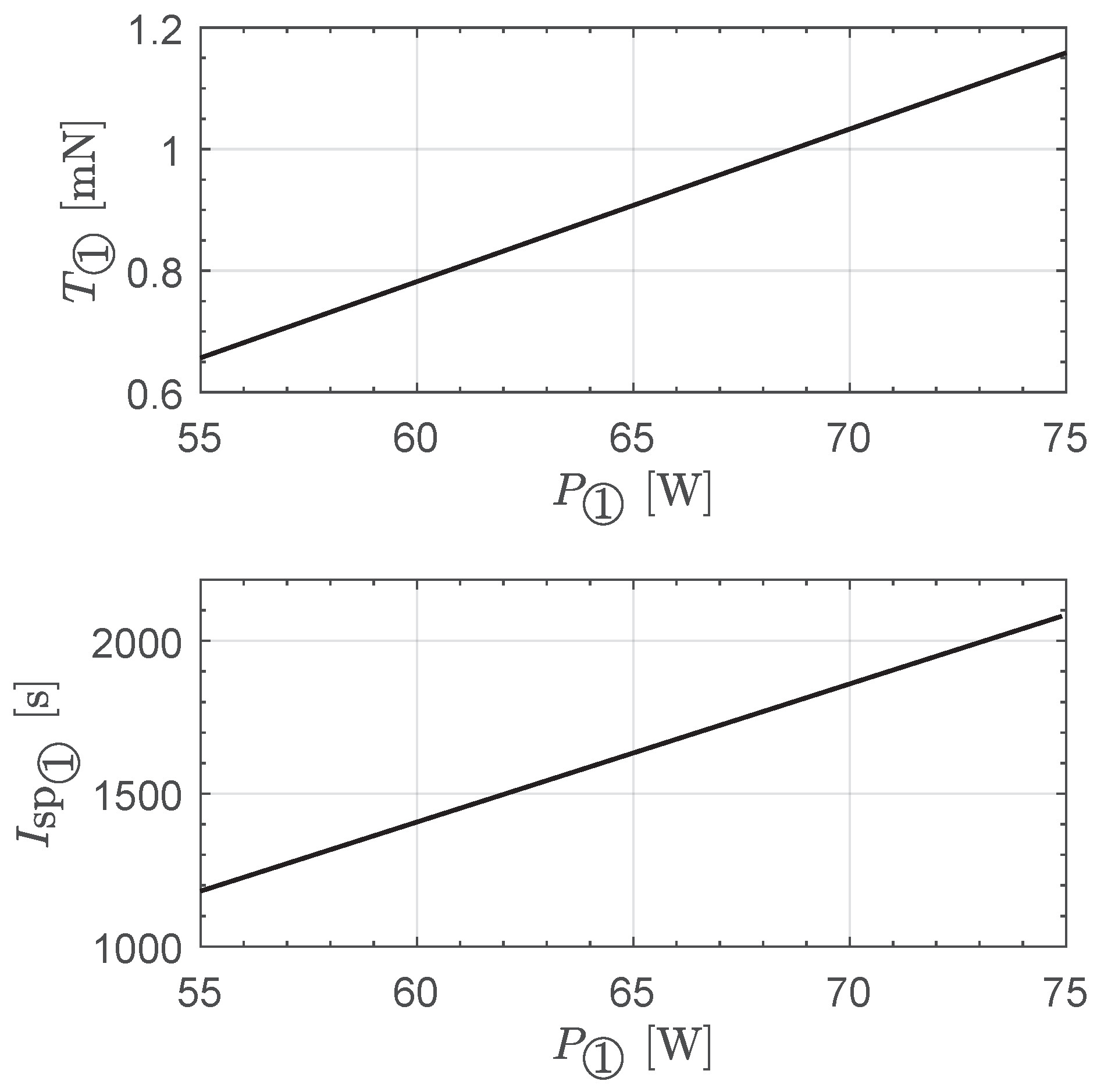
2.1. Thrust Model of a Single Engine Unit Based on the BIT-3 Performance
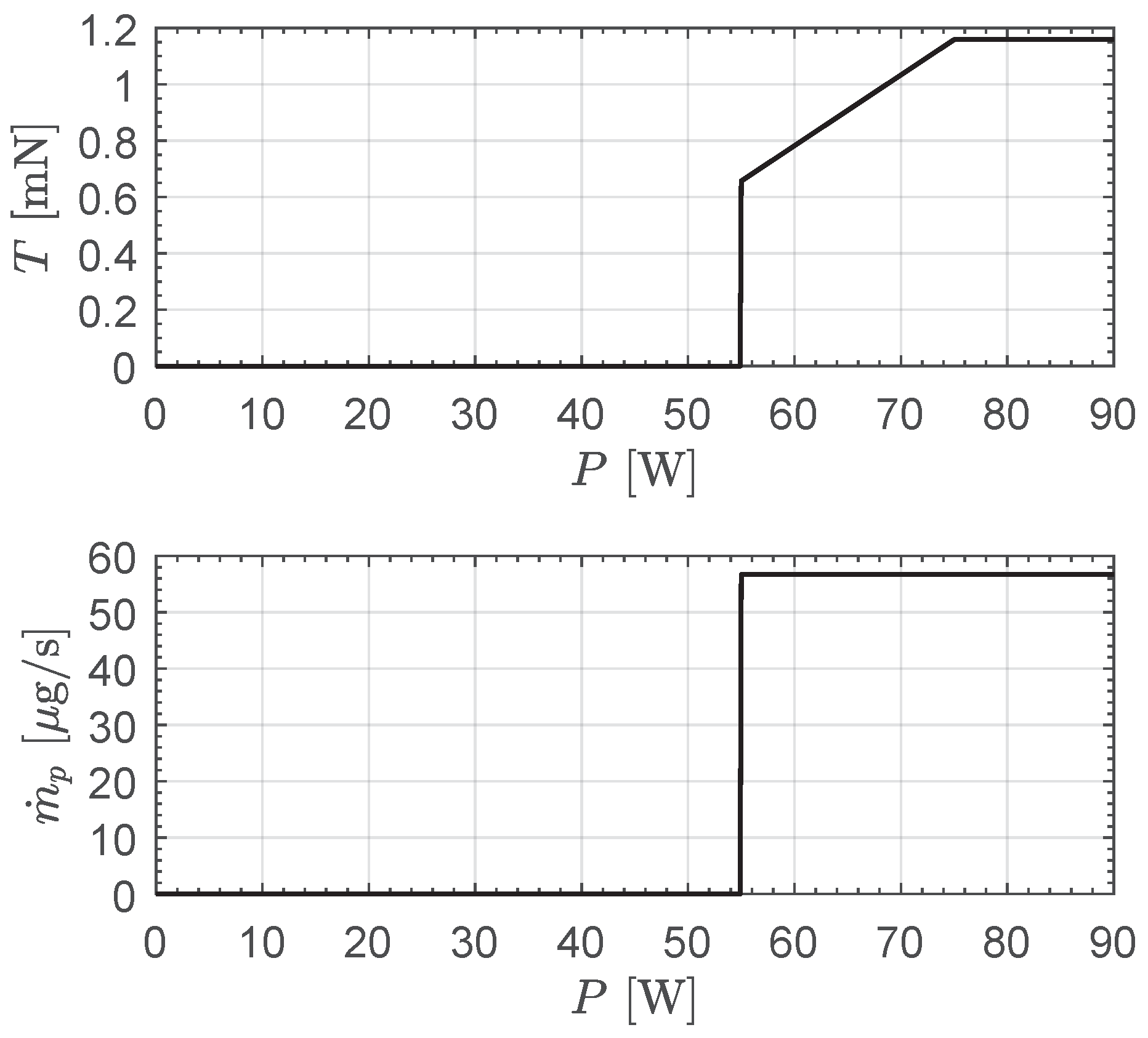
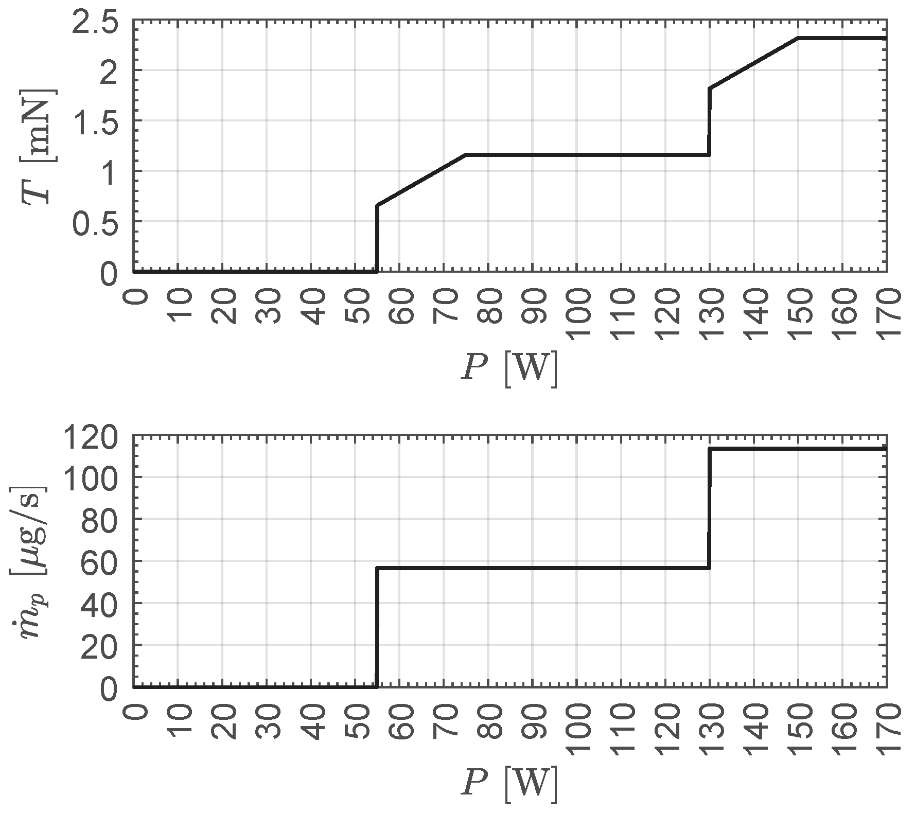
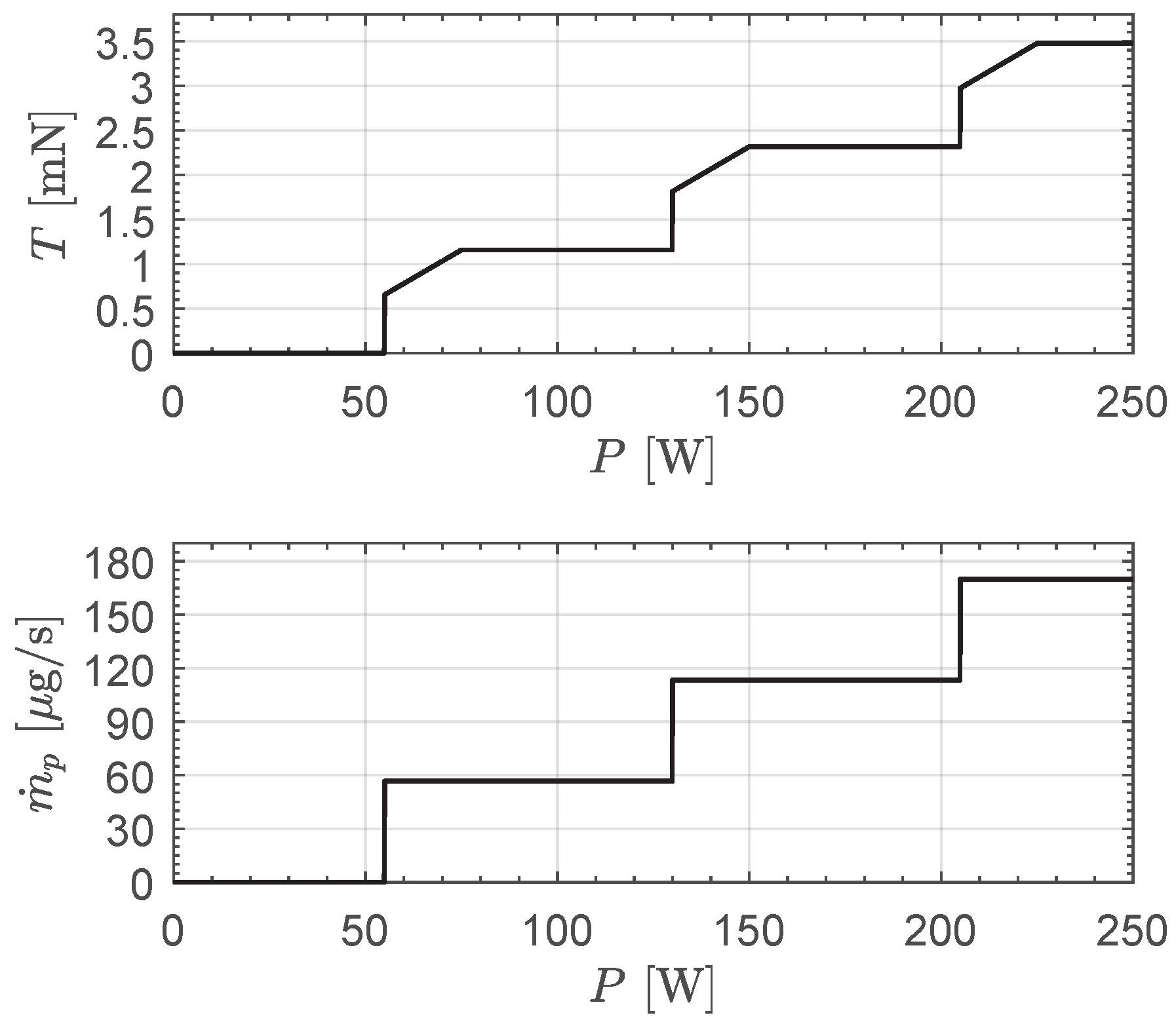
2.2. Thrust Model of an Array of Engines
2.2.1. Case of
2.2.2. Case of
2.2.3. Case of
2.2.4. Case of
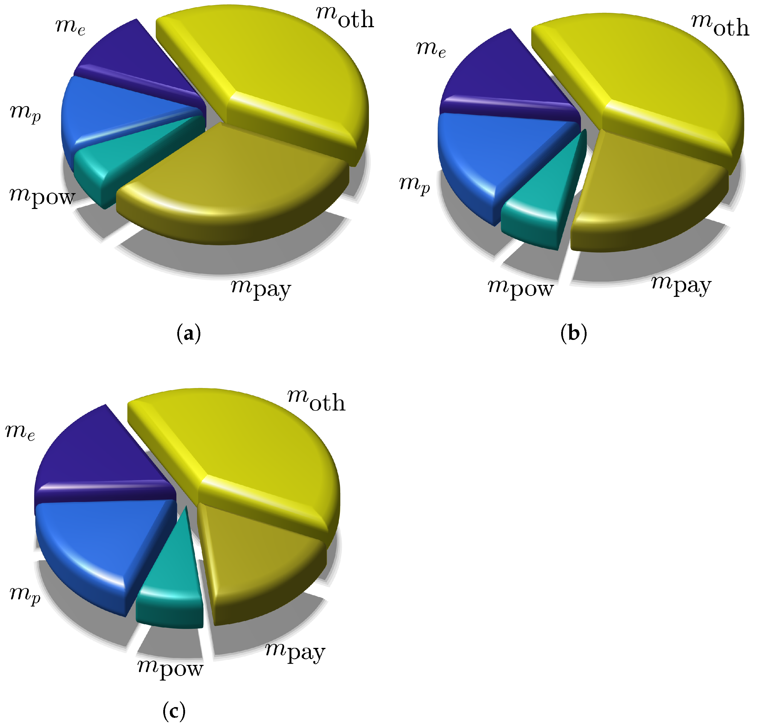
2.3. CubeSat Mass Breakdown and Power Model
3. Heliocentric Trajectory Design and Optimal Guidance Law
4. Numerical Results
5. Potential Mission Applications
6. Conclusions
Funding
Data Availability Statement
Acknowledgments
Conflicts of Interest
Nomenclature
| best fit coefficients for the thrust magnitude; see Equation (1) | |
| best fit coefficients for the specific impulse; see Equation (2) | |
| standard gravity [m/s2] | |
| k | dimensionless contingency factor |
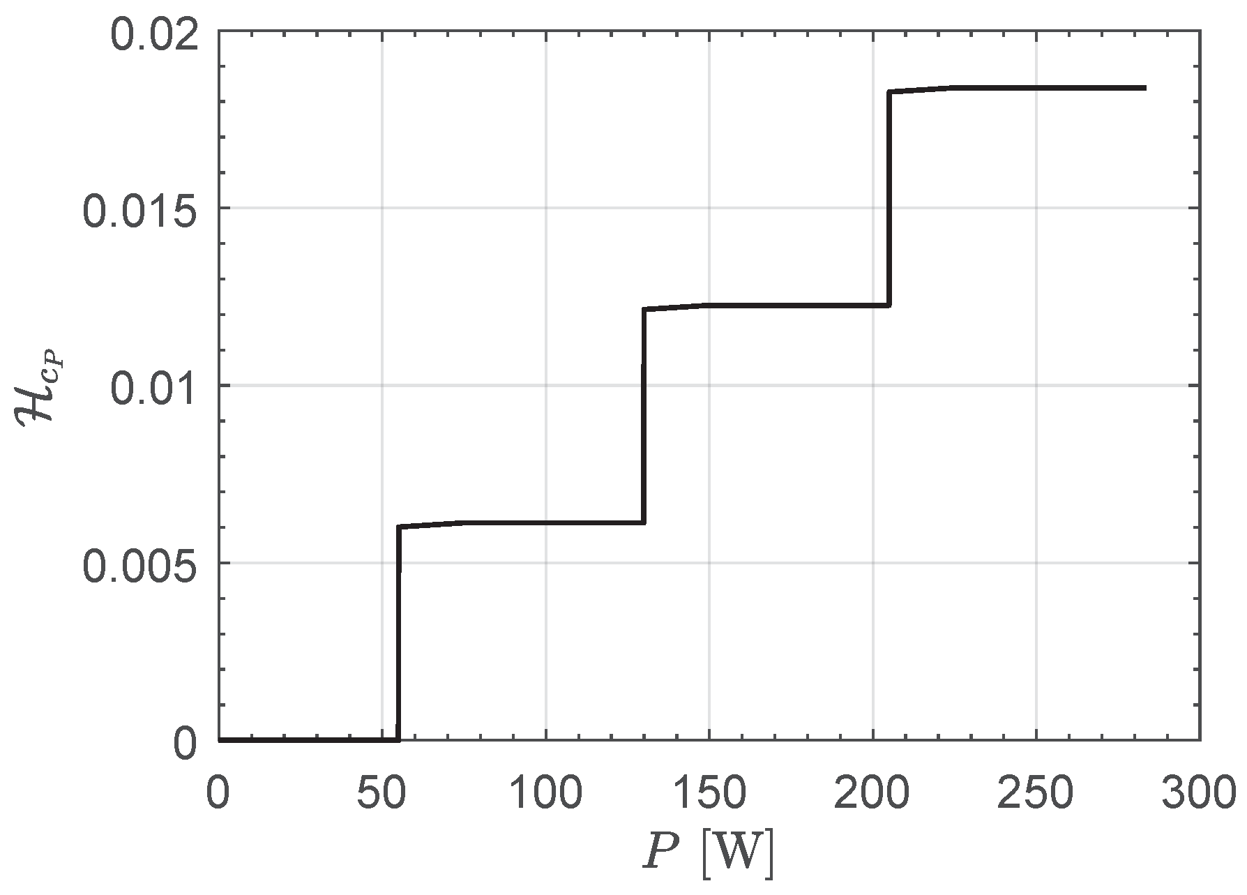
| dimensionless Hamiltonian function | |
| specific impulse [s] | |
| J | performance index [days] |
| m | mass [kg] |
| propellant mass flow rate [kg/s] | |
| N | number of miniaturized thrusters in the array |
| P | power-processing unit input power [W] |
| payload power [W] | |
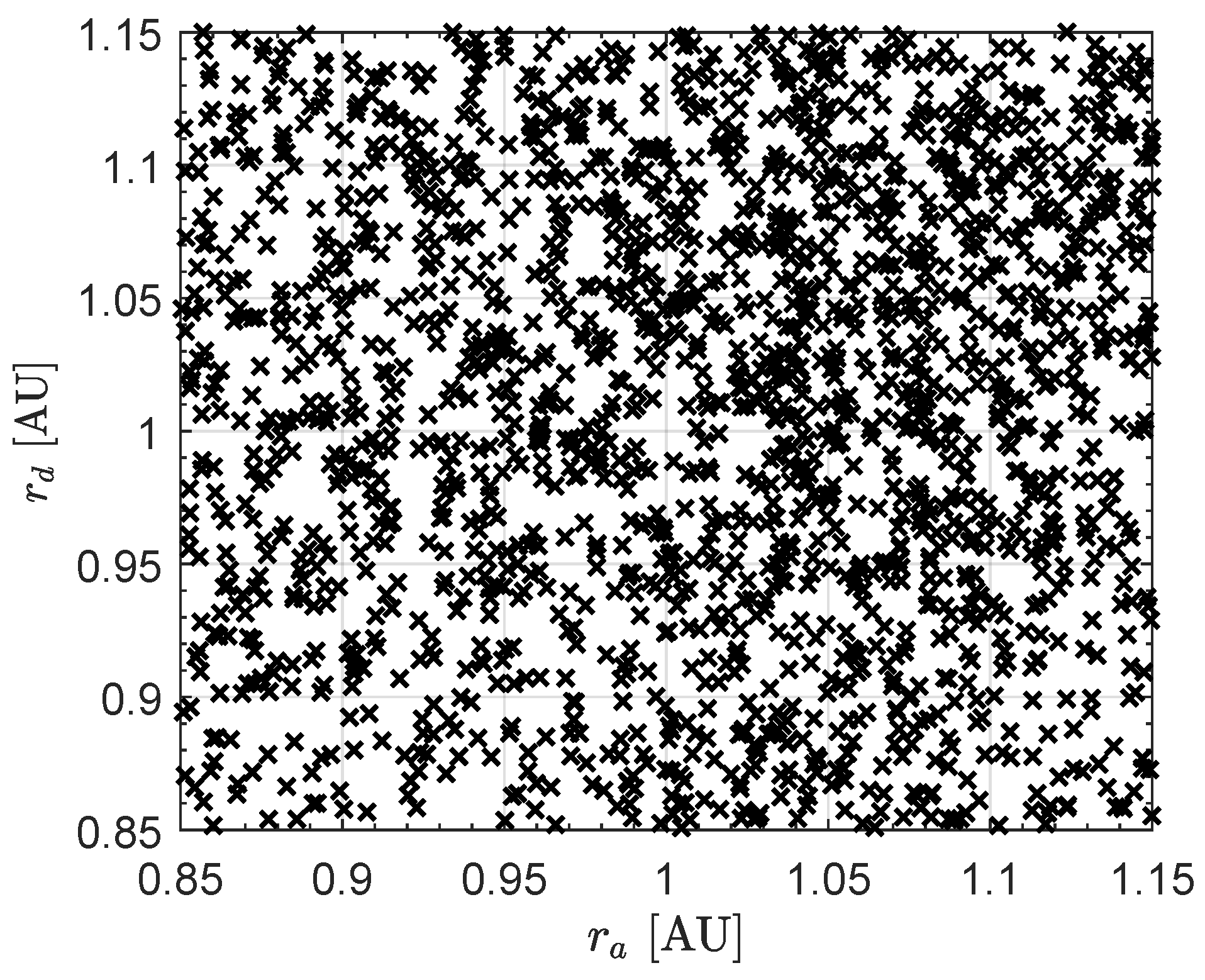
| r | Sun-spacecraft distance [AU] |
| T | thrust magnitude [N] |
| thrust vector [N] | |
| t | time [days] |
| u | radial component of the spacecraft velocity [km/s] |
| v | transverse component of the spacecraft velocity [km/s] |
| Sun’s gravitational parameter [km3/s2] | |
| thrust angle [deg] | |
| reference value of the propellant mass flow rate [kg/s] | |
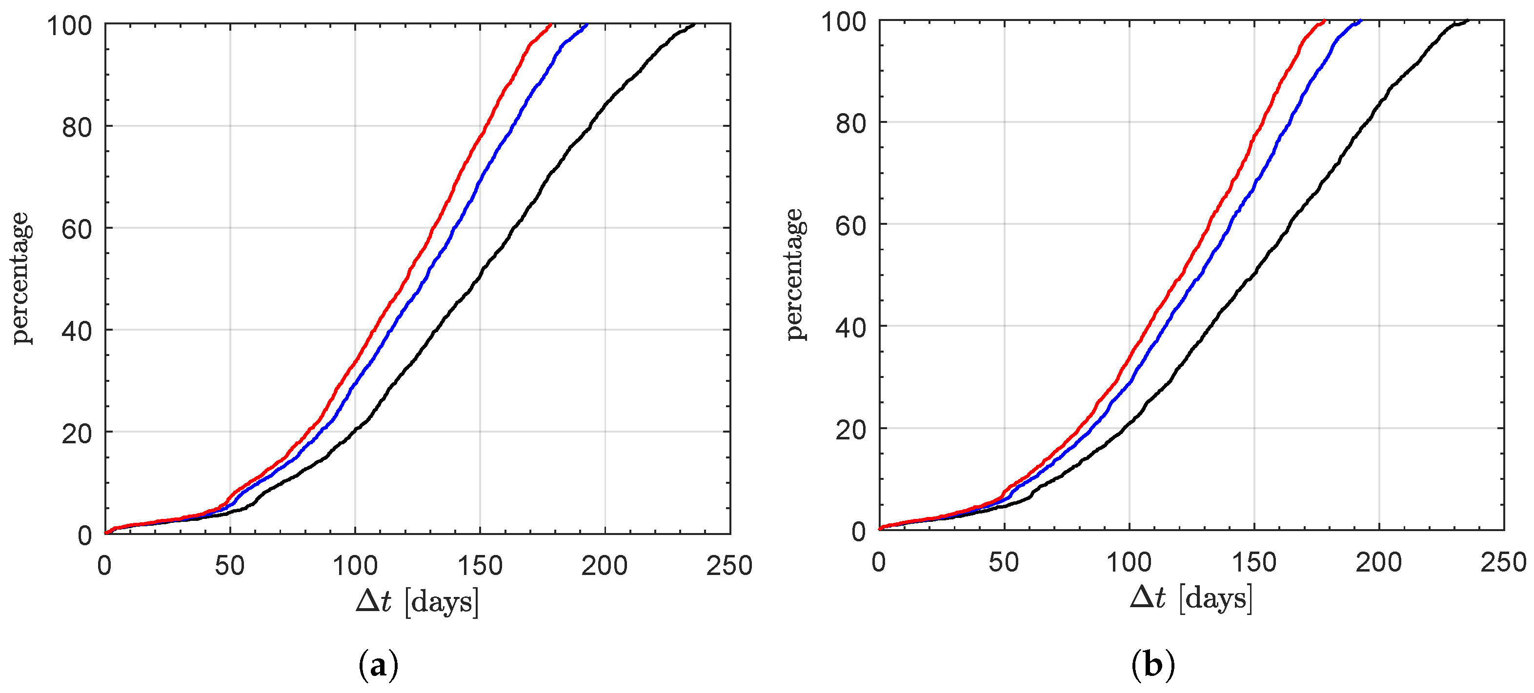
| total flight time [days] | |
| power-to-mass ratio [W/kg] | |
| dimensionless variable adjoint to i-th dimensionless spacecraft state | |
| azimuthal angle [deg] | |
| Subscripts | |
| referred to a single engine unit | |
| 0 | initial, parking orbit |
| ⊕ | at 1 astronomical unit from the Sun |
| available value | |
| e | electric engine dry |
| f | final, target point |
| max | maximum value |
| min | minimum value |
| other subsystems | |
| payload | |
| power generation subsystem | |
| p | propellant |
| Superscripts | |
| · | derivative with respect to t |
| ′ | derivative with respect to |
| ∼ | dimensionless version of the term |
| ∧ | unit vector |
References
- Du, Z.; Jiang, H.; Yang, X.; Cheng, H.W.; Liu, J. Deep learning-assisted near-Earth asteroid tracking in astronomical images. Adv. Space Res. 2024, 73, 5349–5362. [Google Scholar] [CrossRef]
- Assafin, M. Astrometry with PRAIA. Planet. Space Sci. 2023, 238, 105801. [Google Scholar] [CrossRef]
- Mitchell, A.M.; Panicucci, P.; Franzese, V.; Topputo, F.; Linares, R. Improved detection of a Near-Earth Asteroid from an interplanetary CubeSat mission. Acta Astronaut. 2024, 223, 685–692. [Google Scholar] [CrossRef]
- Topputo, F.; Wang, Y.; Giordano, C.; Franzese, V.; Goldberg, H.; Perez-Lissi, F.; Walker, R. Envelop of reachable asteroids by M-ARGO CubeSat. Adv. Space Res. 2021, 67, 4193–4221. [Google Scholar] [CrossRef]
- Pezent, J.; Sood, R.; Heaton, A. High-fidelity contingency trajectory design and analysis for NASA’s near-earth asteroid (NEA) Scout solar sail Mission. Acta Astronaut. 2019, 159, 385–396. [Google Scholar] [CrossRef]
- Ferrari, F.; Franzese, V.; Pugliatti, M.; Giordano, C.; Topputo, F. Preliminary mission profile of Hera’s Milani CubeSat. Adv. Space Res. 2021, 67, 2010–2029. [Google Scholar] [CrossRef]
- Johnson, L.; Castillo-Rogez, J.; Lockett, T. Near Earth asteroid Scout: Exploring asteroid 1991VG using a Smallsat. In Proceedings of the 70th International Astronautical Congress, Washington, DC, USA, 21–25 October 2019. [Google Scholar]
- Franzese, V.; Topputo, F. Celestial Bodies Far-Range Detection with Deep-Space CubeSats. Sensors 2023, 23, 4544. [Google Scholar] [CrossRef] [PubMed]
- Gutierrez, G.; Riccobono, D.; Bruno, E.; Bonariol, T.; Vigna, L.; Reverberi, G.; Fazzoletto, E.; Cotugno, B.; Vitiello, A.; Saita, G.; et al. LICIACube: Mission Outcomes of Historic Asteroid Fly-By Performed by a CubeSat. In Proceedings of the 2024 IEEE Aerospace Conference, Big Sky, MT, USA, 2–9 March 2024. [Google Scholar] [CrossRef]
- Elisabetta, D.; Angelo, Z. Impact observations of asteroid Dimorphos via Light Italian CubeSat for imaging of asteroids (LICIACube). Nat. Commun. 2023, 14, 3055. [Google Scholar] [CrossRef]
- Malphrus, B.K.; Freeman, A.; Staehle, R.; Klesh, A.T.; Walker, R. Interplanetary CubeSat missions. In CubeSat Handbook: From Mission Design to Operations; Cappelletti, C., Battistini, S., Malphrus, B.K., Eds.; Academic Press: London, UK, 2021; Chapter 4; pp. 85–121. [Google Scholar] [CrossRef]
- Zeedan, A.; Khattab, T. CubeSat Communication Subsystems: A Review of On-Board Transceiver Architectures, Protocols, and Performance. IEEE Access 2023, 11, 88161–88183. [Google Scholar] [CrossRef]
- Francisco, C.; Henriques, R.; Barbosa, S. A Review on CubeSat Missions for Ionospheric Science. Aerospace 2023, 10, 622. [Google Scholar] [CrossRef]
- Abbasy, M.; Aghayi Motaaleghi, M. Present the System Design Process and Review of Specifications of a Very Low-Cost 6U CubeSat Platform to Improve Accessibility to Space Based on Pluto Experience. Adv. Astronaut. Sci. Technol. 2023, 6, 1–18. [Google Scholar] [CrossRef]
- Dotto, E.; Deshapriya, J.; Gai, I.; Hasselmann, P.; Mazzotta Epifani, E.; Poggiali, G.; Rossi, A.; Zanotti, G.; Zinzi, A.; Bertini, I.; et al. The Dimorphos ejecta plume properties revealed by LICIACube. Nature 2024, 627, 505–509. [Google Scholar] [CrossRef]
- Deshapriya, J.; Hasselmann, P.; Gai, I.; Hirabayashi, M.; Dotto, E.; Rossi, A.; Zinzi, A.; Corte, V.D.; Bertini, I.; Ieva, S.; et al. Characterization of the DART Impact Ejecta Plume on Dimorphos from LICIACube Observations. Planet. Sci. J. 2023, 4, 231. [Google Scholar] [CrossRef]
- Klesh, A.T. MARCO: Flight results from the first interplanetary CubeSat mission. In Proceedings of the 70th Annual International Astronautical Congress, Washington, DC, USA, 21–25 October 2019. [Google Scholar]
- Schoolcraft, J.; Klesh, A.; Werne, T. MarCO: Interplanetary Mission Development on a CubeSat Scale. In Space Operations: Contributions from the Global Community; Springer International Publishing: Berlin/Heidelberg, Germany, 2017; Chapter 10; pp. 221–231. [Google Scholar] [CrossRef]
- Schoolcraft, J.; Klesh, A.T.; Werne, T. MarCO: Interplanetary mission development on a cubesat scale. In Proceedings of the SpaceOps 2016 Conference, Daejeon, Republic of Korea, 16–20 May 2016. [Google Scholar] [CrossRef]
- Kulu, E. Nanosatellite Launch Forecasts - Track Record and Latest Prediction. In Proceedings of the 36th Annual Small Satellite Conference, Logan, UT, USA, 6–11 August 2022. [Google Scholar]
- Freeman, A.; Malphrus, B.K.; Staehle, R. CubeSat science instruments. In CubeSat Handbook: From Mission Design to Operations; Cappelletti, C., Battistini, S., Malphrus, B.K., Eds.; Academic Press: London, UK, 2021; Chapter 3; pp. 67–83. [Google Scholar] [CrossRef]
- Barán, B.; Martínez, B.O.; Barán, M. Multi-objective Optimization in the selection of a CubeSat PayLoad. In Proceedings of the 2021 IEEE International Conference on Aerospace and Signal Processing (INCAS 2021), Lima, Peru, 28–30 November 2021. [Google Scholar] [CrossRef]
- Aziz, M.M.; Ong, W.N.; Edwar; Fitriyanti, L.K.; Saugi, I.H.; Hidayat, F.A. Preliminary design of cubesat payload for clouds coverage detection using RGB camera. In Proceedings of the The 8th International Seminar on Aerospace Science and Technology (ISAST 2020), Bogor, Indonesia, 17 November 2021; Volume 2366. [Google Scholar] [CrossRef]
- Anderson, L.; Mork, J.; Swenson, C.; Zwolinski, B.; Mastropietro, A.J.; Sauder, J.; McKinley, I.; Mok, M. CubeSat active thermal control in support of advanced payloads: The active thermal architecture project. In Proceedings of the SPIE—The International Society for Optical Engineering, San Diego, CA, USA, 1–5 August 2021. [Google Scholar] [CrossRef]
- Garranzo, D.; Núñez, A.; Laguna, H.; Belenguer, T.; De Miguel, E.; Cebollero, M.; Ibarmia, S.; Martínez, C. APIS: The miniaturized Earth observation camera on-board OPTOS CubeSat. J. Appl. Remote Sens. 2019, 13, 032502. [Google Scholar] [CrossRef]
- Dalbins, J.; Allaje, K.; Ehrpais, H.; Iakubivskyi, I.; Ilbis, E.; Janhunen, P.; Kivastik, J.; Merisalu, M.; Noorma, M.; Pajusalu, M.; et al. Interplanetary student nanospacecraft: Development of the LEO demonstrator ESTCube-2. Aerospace 2023, 10, 503. [Google Scholar] [CrossRef]
- Staehle, R.; Blaney, D.; Hemmati, H.; Jones, D.; Klesh, A.; Liewer, P.; Lazio, J.; Wen-Yu Lo, M.; Mouroulis, P.; Murphy, N.; et al. Interplanetary CubeSat Architecture and Missions. In Proceedings of the AIAA SPACE 2012 Conference & Exposition, Pasadena, CA, USA, 11–13 September 2012. [Google Scholar] [CrossRef]
- Alnaqbi, S.; Darfilal, D.; Swei, S.S.M. Propulsion Technologies for CubeSats: Review. Aerospace 2024, 11, 502. [Google Scholar] [CrossRef]
- Kabirov, V.; Semenov, V.; Torgaeva, D.; Otto, A. Miniaturization of spacecraft electrical power systems with solar-hydrogen power supply system. Int. J. Hydrogen Energy 2023, 48, 9057–9070. [Google Scholar] [CrossRef]
- Yeo, S.H.; Ogawa, H.; Kahnfeld, D.; Schneider, R. Miniaturization perspectives of electrostatic propulsion for small spacecraft platforms. Prog. Aerosp. Sci. 2021, 126, 100742. [Google Scholar] [CrossRef]
- Wright, W.; Ferrer, P. Electric micropropulsion systems. Prog. Aerosp. Sci. 2015, 74, 48–61. [Google Scholar] [CrossRef]
- Yeo, S.H.; Gadisa, D.; Ogawa, H.; Bang, H. Multi-objective design optimization and physics-based sensitivity analysis of field emission electric propulsion for CubeSat platforms. Aerosp. Sci. Technol. 2024, 154, 109516. [Google Scholar] [CrossRef]
- Stesina, F.; Corpino, S.; Borras, E.B.; Amo, J.G.D.; Pavarin, D.; Bellomo, N.; Trezzolani, F. Environmental test campaign of a 6U CubeSat Test Platform equipped with an ambipolar plasma thruster. Adv. Aircr. Spacecr. Sci. 2022, 9, 195–215. [Google Scholar] [CrossRef]
- Bellomo, N.; Magarotto, M.; Manente, M.; Trezzolani, F.; Mantellato, R.; Cappellini, L.; Paulon, D.; Selmo, A.; Scalzi, D.; Minute, M.; et al. Design and In-orbit Demonstration of REGULUS, an Iodine electric propulsion system. CEAS Space J. 2022, 14, 79–90. [Google Scholar] [CrossRef]
- Lockett, T.R.; Castillo-Rogez, J.; Johnson, L.; Matus, J.; Lightholder, J.; Marinan, A.; Few, A. Near-Earth Asteroid Scout Flight Mission. IEEE Aerosp. Electron. Syst. Mag. 2020, 35, 20–29. [Google Scholar] [CrossRef]
- Heaton, A.; Miller, K.; Ahmad, N. Near earth asteroid Scout solar sail thrust and torque model. In Proceedings of the 4th International Symposium on Solar Sailing (ISSS 2017), Kyoyo, Japan, 17–20 January 2017. [Google Scholar]
- McNutt, L.; Johnson, L.; Clardy, D.; Castillo-Rogez, J.; Frick, A.; Jones, L. Near-earth asteroid scout. In Proceedings of the AIAA SPACE 2014 Conference and Exposition, San Diego, CA, USA, 4–7 August 2014. [Google Scholar]
- Quarta, A.A. Continuous-Thrust Circular Orbit Phasing Optimization of Deep Space CubeSats. Appl. Sci. 2024, 14, 7059. [Google Scholar] [CrossRef]
- Franzese, V.; Topputo, F.; Ankersen, F.; Walker, R. Deep-Space Optical Navigation for M-ARGO Mission. J. Astronaut. Sci. 2021, 68, 1034–1055. [Google Scholar] [CrossRef]
- Franzese, V.; Giordano, C.; Wang, Y.; Topputo, F.; Goldberg, H.; Gonzalez, A.; Walker, R. Target selection for M-ARGO interplanetary cubesat. In Proceedings of the 71st International Astronautical Congress, Virtual Event, 12–14 October 2020. [Google Scholar]
- Quarta, A.A. Thrust model and trajectory design of an interplanetary CubeSat with a hybrid propulsion system. Actuators 2024, 13, 384. [Google Scholar] [CrossRef]
- Perozzi, E.; Rossi, A.; Valsecchi, G.B. Basic targeting strategies for rendezvous and flyby missions to the near-Earth asteroids. Planet. Space Sci. 2001, 49, 3–22. [Google Scholar] [CrossRef]
- Mengali, G.; Bassetto, M.; Quarta, A.A. Solar Sail Optimal Performance in Heliocentric Nodal Flyby Missions. Aerospace 2024, 11, 427. [Google Scholar] [CrossRef]
- Mengali, G.; Quarta, A.A. Optimal Nodal Flyby with Near-Earth Asteroids Using Electric Sail. Acta Astronaut. 2014, 104, 450–457. [Google Scholar] [CrossRef]
- Janhunen, P. Electric sail for spacecraft propulsion. J. Propuls. Power 2004, 20, 763–764. [Google Scholar] [CrossRef]
- Janhunen, P.; Toivanen, P.K.; Polkko, J.; Merikallio, S.; Salminen, P.; Haeggström, E.; Seppänen, H.; Kurppa, R.; Ukkonen, J.; Kiprich, S.; et al. Electric solar wind sail: Toward test missions. Rev. Sci. Instruments 2010, 81, 111301. [Google Scholar] [CrossRef] [PubMed]
- Palos, M.F.; Janhunen, P.; Toivanen, P.; Tajmar, M.; Iakubivskyi, I.; Micciani, A.; Orsini, N.; Kütt, J.; Rohtsalu, A.; Dalbins, J.; et al. Electric Sail Mission Expeditor, ESME: Software Architecture and Initial ESTCube Lunar Cubesat E-sail Experiment Design. Aerospace 2023, 10, 694. [Google Scholar] [CrossRef]
- Tsay, M.; Frongillo, J.; Model, J.; Zwahlen, J.; Barcroft, C.; Feng, C. Neutralization demo and thrust stand measurement for BIT-3 RF ion thruster. In Proceedings of the 53rd AIAA/SAE/ASEE Joint Propulsion Conference, Atlanta, GA, USA, 10–12 July 2017. [Google Scholar] [CrossRef]
- Tsay, M.; Frongillo, J.; Model, J.; Zwahlen, J.; Paritsky, L. Maturation of iodine-fueled BIT-3 RF ion thruster and RF neutralizer. In Proceedings of the 52nd AIAA/SAE/ASEE Joint Propulsion Conference, Salt Lake City, UT, USA, 25–27 July 2016. [Google Scholar] [CrossRef]
- Malphrus, B.K.; Brown, K.Z.; Garcia, J.; Conner, C.; Kruth, J.; Combs, M.S.; Fite, N.; McNeil, S.; Clark, P.; Angkasa, K.; et al. Lunar IceCube: Pioneering technologies for interplanetary small satellite exploration. In Proceedings of the 70th International Astronautical Congress (IAC), Washington, DC, USA, 21–25 October 2019. [Google Scholar]
- Lane, R.; Ryals, C.; McLemore, C.; Hitt, D. NASA Space Launch System Cubesats: First Flight and Future Opportunities. In Proceedings of the 37th Annual Small Satellite Conference, Logan, UT, USA, 5–10 August 2023. [Google Scholar]
- McNaul, E. HaWK Solar Array Technology Advanced Deployable Satellite Power Solution. In Proceedings of the 12th Annual Summer CubeSat Developers’ Workshop, Logan, UT, USA, 8–9 August 2015. [Google Scholar]
- Betts, J.T. Survey of Numerical Methods for Trajectory Optimization. J. Guid. Control Dyn. 1998, 21, 193–207. [Google Scholar] [CrossRef]
- Chai, R.; Savvaris, A.; Tsourdos, A.; Chai, S.; Xia, Y. A review of optimization techniques in spacecraft flight trajectory design. Prog. Aerosp. Sci. 2019, 109, 100543. [Google Scholar] [CrossRef]
- Shirazi, A.; Ceberio, J.; Lozano, J.A. Spacecraft trajectory optimization: A review of models, objectives, approaches and solutions. Prog. Aerosp. Sci. 2018, 102, 76–98. [Google Scholar] [CrossRef]
- Ross, I.M. A Primer on Pontryagin’s Principle in Optimal Control; Collegiate Publishers: San Francisco, CA, USA, 2015; Chapter 2; pp. 127–129. [Google Scholar]
- Lawden, D.F. Optimal Trajectories for Space Navigation; Butterworths & Co., Inc.: London, UK, 1963; pp. 54–60. [Google Scholar]
- Busek Co., Inc. BIT-3: Compact and Efficient Iodine Gridded Ion Thruster. 2024. Available online: https://www.busek.com/bit3 (accessed on 12 December 2024).
- Sutton, G.P. Rocket Propulsion Elements; John Wiley & Sons Inc.: Danvers, MA, USA, 2017; Chapter 2; pp. 26–31. [Google Scholar]
- Takao, Y.; Mori, O.; Matsushita, M.; Sugihara, A.K. Solar electric propulsion by a solar power sail for small spacecraft missions to the outer solar system. Acta Astronaut. 2021, 181, 362–376. [Google Scholar] [CrossRef]
- Takao, Y.; Mori, O.; Matsumoto, J.; Chujo, T.; Kikuchi, S.; Kebukawa, Y.; Ito, M.; Okada, T.; Aoki, J.; Yamada, K.; et al. Sample return system of OKEANOS–The solar power sail for Jupiter Trojan exploration. Acta Astronaut. 2023, 213, 121–137. [Google Scholar] [CrossRef]
- Berthet, M.; Schalkwyk, J.; Çelik, O.; Sengupta, D.; Fujino, K.; Hein, A.M.; Tenorio, L.; Cardoso dos Santos, J.; Worden, S.P.; Mauskopf, P.D.; et al. Space sails for achieving major space exploration goals: Historical review and future outlook. Prog. Aerosp. Sci. 2024, 150, 101047. [Google Scholar] [CrossRef]
- MMA Space. MMA HaWK Solar Arrays. 2024. Available online: https://mmadesignllc.com/next-gen-solar-arrays/ (accessed on 12 December 2024).
- Quarta, A.A.; Mengali, G. Minimum-Time Space Missions with Solar Electric Propulsion. Aerosp. Sci. Technol. 2011, 15, 381–392. [Google Scholar] [CrossRef]
- Mengali, G.; Quarta, A.A. Optimal trade studies of interplanetary electric propulsion missions. Acta Astronaut. 2008, 62, 657–667. [Google Scholar] [CrossRef]
- Bryson, A.E.; Ho, Y.C. Applied Optimal Control; Hemisphere Publishing Corporation: New York, NY, USA, 1975; Chapter 2; pp. 71–89. ISBN 0-891-16228-3. [Google Scholar]
- Yang, W.Y.; Cao, W.; Kim, J.; Park, K.W.; Park, H.H.; Joung, J.; Ro, J.S.; Hong, C.H.; Im, T. Applied Numerical Methods Using MATLAB; John Wiley & Sons, Inc.: Hoboken, NJ, USA, 2020; Chapters 6 and 7; pp. 312, 378–379. [Google Scholar]
- Shampine, L.F.; Reichelt, M.W. The MATLAB ODE Suite. SIAM J. Sci. Comput. 1997, 18, 1–22. [Google Scholar] [CrossRef]
- Quarta, A.A. Fast initialization of the indirect optimization problem in the solar sail circle-to-circle orbit transfer. Aerosp. Sci. Technol. 2024, 147, 109058. [Google Scholar] [CrossRef]
- Quarta, A.A. Initial costate approximation for rapid orbit raising with very low propulsive acceleration. Appl. Sci. 2024, 14, 1124. [Google Scholar] [CrossRef]
- Mengali, G.; Quarta, A.A. Tradeoff performance of hybrid low-thrust propulsion system. J. Spacecr. Rocket. 2007, 44, 1263–1270. [Google Scholar] [CrossRef]
- NEODyS. Near Earth Objects—Dynamic Site. 2024. Available online: https://newton.spacedys.com/neodys/index.php?pc=5 (accessed on 27 December 2024).
- Curtis, H.D. Orbital Mechanics for Engineering Students; Elsevier: Oxford, UK, 2014; Chapter 6; pp. 298–303. [Google Scholar] [CrossRef]


| N | 1 | 2 | 3 |
|---|---|---|---|
| [kg] | |||
| [kg] | 3 | ||
| [kg] | |||
| [kg] | 4 | 4 | 4 |
| [kg] | |||
| [kg] |
Disclaimer/Publisher’s Note: The statements, opinions and data contained in all publications are solely those of the individual author(s) and contributor(s) and not of MDPI and/or the editor(s). MDPI and/or the editor(s) disclaim responsibility for any injury to people or property resulting from any ideas, methods, instructions or products referred to in the content. |
© 2025 by the author. Licensee MDPI, Basel, Switzerland. This article is an open access article distributed under the terms and conditions of the Creative Commons Attribution (CC BY) license (https://creativecommons.org/licenses/by/4.0/).
Share and Cite
Quarta, A.A. Preliminary Trajectory Analysis of CubeSats with Electric Thrusters in Nodal Flyby Missions for Asteroid Exploration. Remote Sens. 2025, 17, 513. https://doi.org/10.3390/rs17030513
Quarta AA. Preliminary Trajectory Analysis of CubeSats with Electric Thrusters in Nodal Flyby Missions for Asteroid Exploration. Remote Sensing. 2025; 17(3):513. https://doi.org/10.3390/rs17030513
Chicago/Turabian StyleQuarta, Alessandro A. 2025. "Preliminary Trajectory Analysis of CubeSats with Electric Thrusters in Nodal Flyby Missions for Asteroid Exploration" Remote Sensing 17, no. 3: 513. https://doi.org/10.3390/rs17030513
APA StyleQuarta, A. A. (2025). Preliminary Trajectory Analysis of CubeSats with Electric Thrusters in Nodal Flyby Missions for Asteroid Exploration. Remote Sensing, 17(3), 513. https://doi.org/10.3390/rs17030513