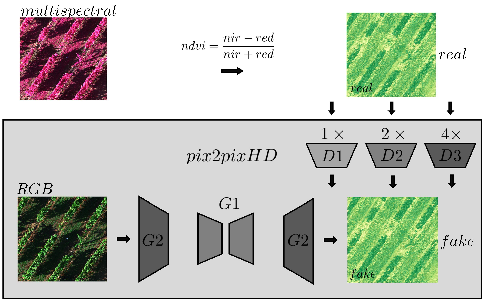
Figure 1.
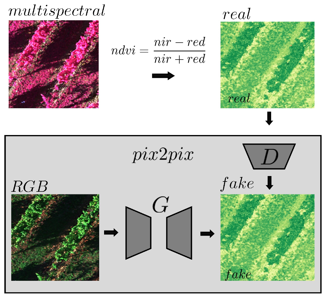
Overview of the Methodology. The process began with dataset preprocessing (
Section 2.2), followed by GAN model training (
Section 2.3), artificial NDVI map reconstruction (
Section 2.4), and finally, model evaluation. The
btg2021 and
btg2022 datasets were acquired at the Bodegas Terras Gaudas vineyard in Spain, with a MicaSense RedEdge, MicaSense Altum-PT and DJI Phantom 4-RTK (RGB) cameras.
can2023, collected at the Canyelles vineyard in Spain using a DJI Mavic 3M multispectral system. Model training resulted in four distinct models, Pix2Pix and Pix2PixHD, trained on either RGB and NDVI pairs, or multispectral composite RGB and NDVI pairs. The evaluation stage included direct pixel-level accuracy assessments (
Section 3.1) across these datasets as well as Botrytis (
Section 3.2) from Ariza-Sentís et al. [
33] and Vigor mapping (
Section 3.3) from Matese et al. [
4].
Figure 1.
Overview of the Methodology. The process began with dataset preprocessing (
Section 2.2), followed by GAN model training (
Section 2.3), artificial NDVI map reconstruction (
Section 2.4), and finally, model evaluation. The
btg2021 and
btg2022 datasets were acquired at the Bodegas Terras Gaudas vineyard in Spain, with a MicaSense RedEdge, MicaSense Altum-PT and DJI Phantom 4-RTK (RGB) cameras.
can2023, collected at the Canyelles vineyard in Spain using a DJI Mavic 3M multispectral system. Model training resulted in four distinct models, Pix2Pix and Pix2PixHD, trained on either RGB and NDVI pairs, or multispectral composite RGB and NDVI pairs. The evaluation stage included direct pixel-level accuracy assessments (
Section 3.1) across these datasets as well as Botrytis (
Section 3.2) from Ariza-Sentís et al. [
33] and Vigor mapping (
Section 3.3) from Matese et al. [
4].
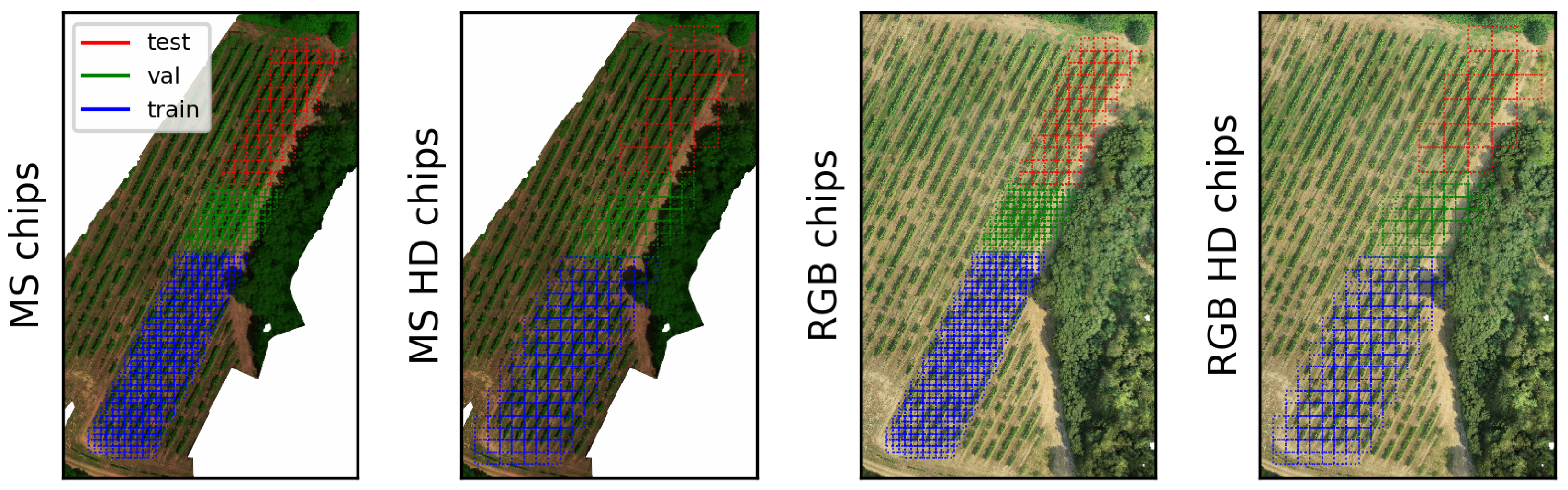
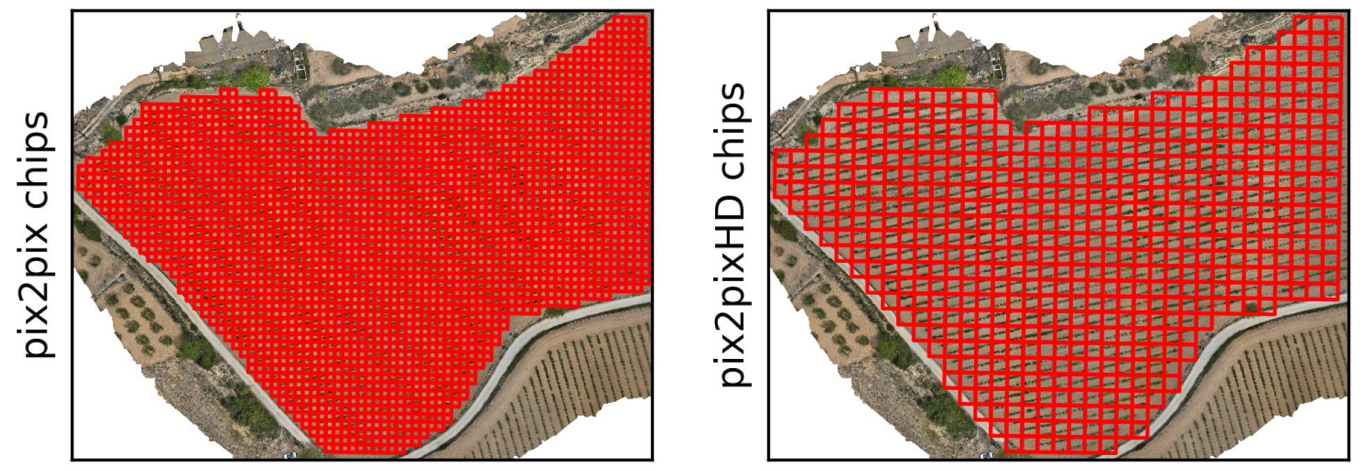
Figure 2.
The btg2022 training, testing and validation chips subsets. Left shows the Pix2Pix chips, at a size of 256 by 256 pixels. The right image shows the Pix2PixHD chips at 512 by 512 pixels. The blue and green squares are the training and validation chips, whereas the red squares are the testing chips. Smaller-looking squares in train and val are due to overlapping chips.
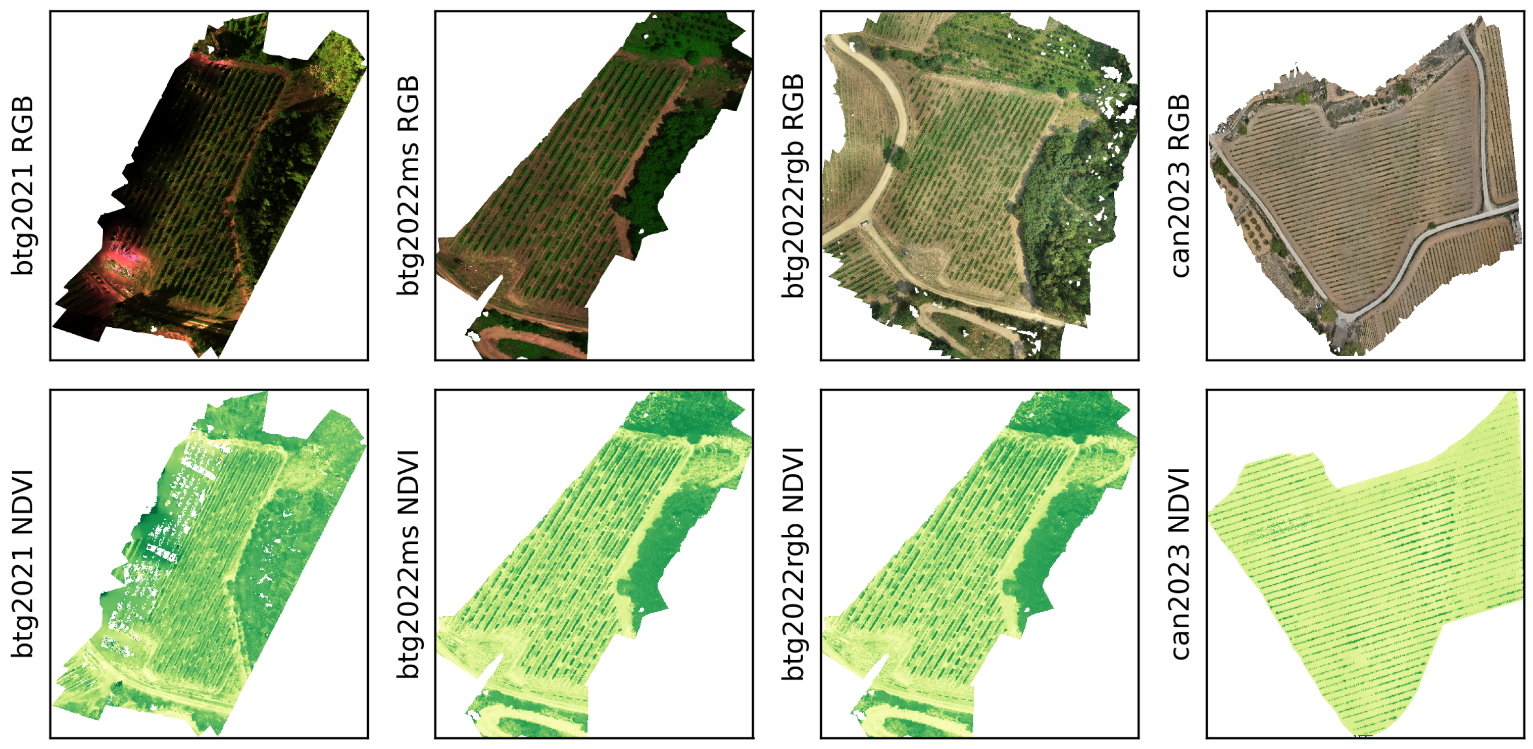
Figure 3.
Visual overview of the btg2021, btg2022ms, btg2022rgb and can2023 orthomosaics before alignment and chipping. The top row visualizes the composite or true RGB for btg2021, btg2022 and can2023. The real NDVI maps are shown on the bottom row.
Figure 3.
Visual overview of the btg2021, btg2022ms, btg2022rgb and can2023 orthomosaics before alignment and chipping. The top row visualizes the composite or true RGB for btg2021, btg2022 and can2023. The real NDVI maps are shown on the bottom row.
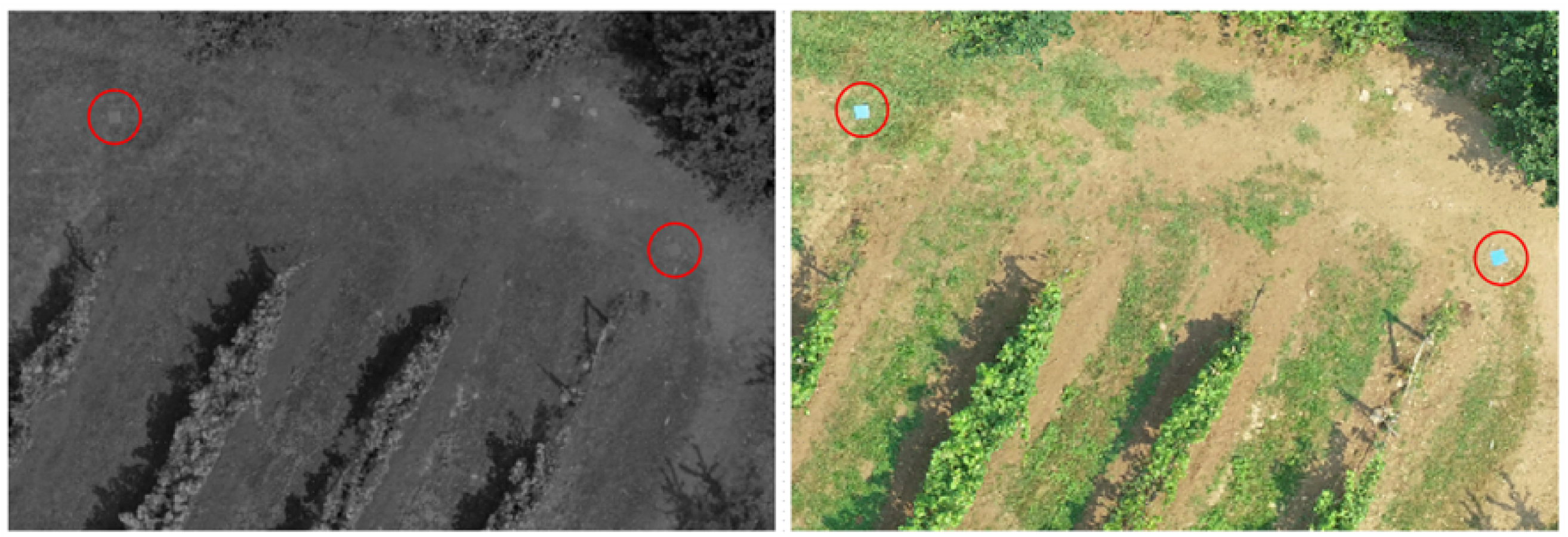
Figure 4.
Example blue tags visible in both btg2022 RGB and MS orthomosaics were used as alignment points. The spatial resolution of the RGB sensor was bi-linearly interpolated to match the MS resolution.
Figure 4.
Example blue tags visible in both btg2022 RGB and MS orthomosaics were used as alignment points. The spatial resolution of the RGB sensor was bi-linearly interpolated to match the MS resolution.
Figure 5.
Cross-validation results and model selection based on MSE results on the validation dataset. The green lines indicate the mean. The red box shows the selected model from the training procedure. Sub-figures (a–d) show the performance of four candidate models during cross-validation, highlighting the differences in MSE values. These results were used to guide model selection for optimal performance.
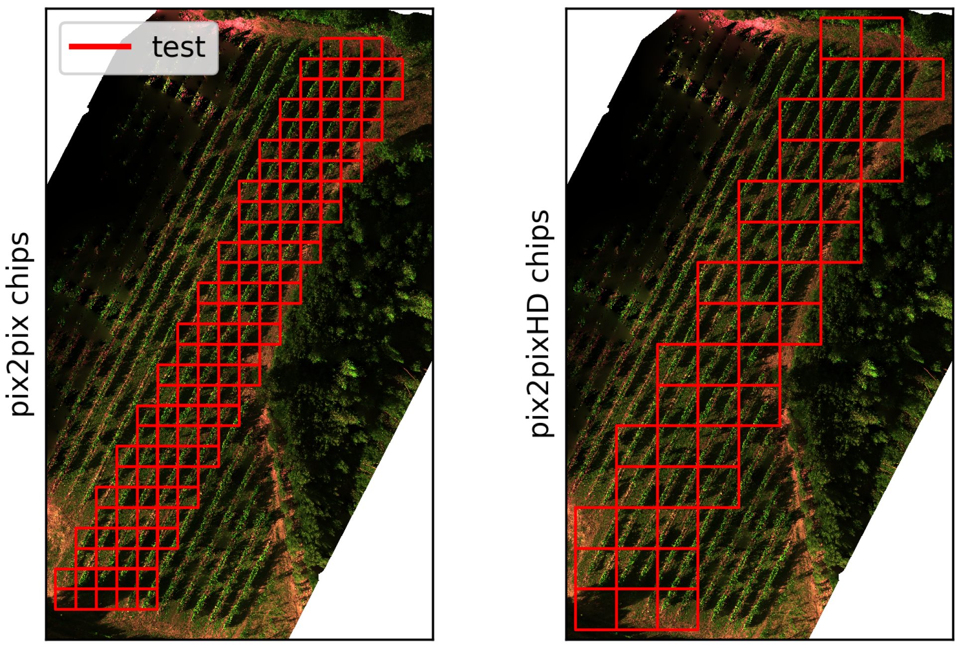
Figure 6.
The location of the testing chips in the btg2021 dataset. Left shows the smaller Pix2Pix chips, with chips at a resolution of 256 by 256 pixels. Right shows the Pix2PixHD chips, with chips at a resolution of 512 by 512 pixels.
Figure 6.
The location of the testing chips in the btg2021 dataset. Left shows the smaller Pix2Pix chips, with chips at a resolution of 256 by 256 pixels. Right shows the Pix2PixHD chips, with chips at a resolution of 512 by 512 pixels.
Figure 7.
The location of the testing chips in the can2023 dataset. Left shows the smaller Pix2Pix chips, with chips at a resolution of 256 by 256 pixels. Right shows the Pix2PixHD chips, with chips at a resolution of 512 by 512 pixels.
Figure 7.
The location of the testing chips in the can2023 dataset. Left shows the smaller Pix2Pix chips, with chips at a resolution of 256 by 256 pixels. Right shows the Pix2PixHD chips, with chips at a resolution of 512 by 512 pixels.
Figure 8.
Processing flowchart for pixel-level accuracies. In the pre-processing step, the earlier steps are performed, and the real and artificial NDVI orthomosaics are generated. Which is directly used to calculate the SSIM and PSNR values. These arrays are then flattened into a list for MSE and R-squared.
Figure 9.
Processing flowchart for Botrytis Bunch Rot Risk (BBR) mapping. In the pre-processing step, the orthomosaic photogrammetric reconstruction, digital surface model (DSM) creation and the real and artificial NDVI orthomosaics were generated. The red band was used to identify the shadow-pixels and is a direct measure of leaf area index, the DSM was further processed to acquire a canopy height model. These products were then placed into the BBR algorithm from Ariza-Sentís et al. [
33].
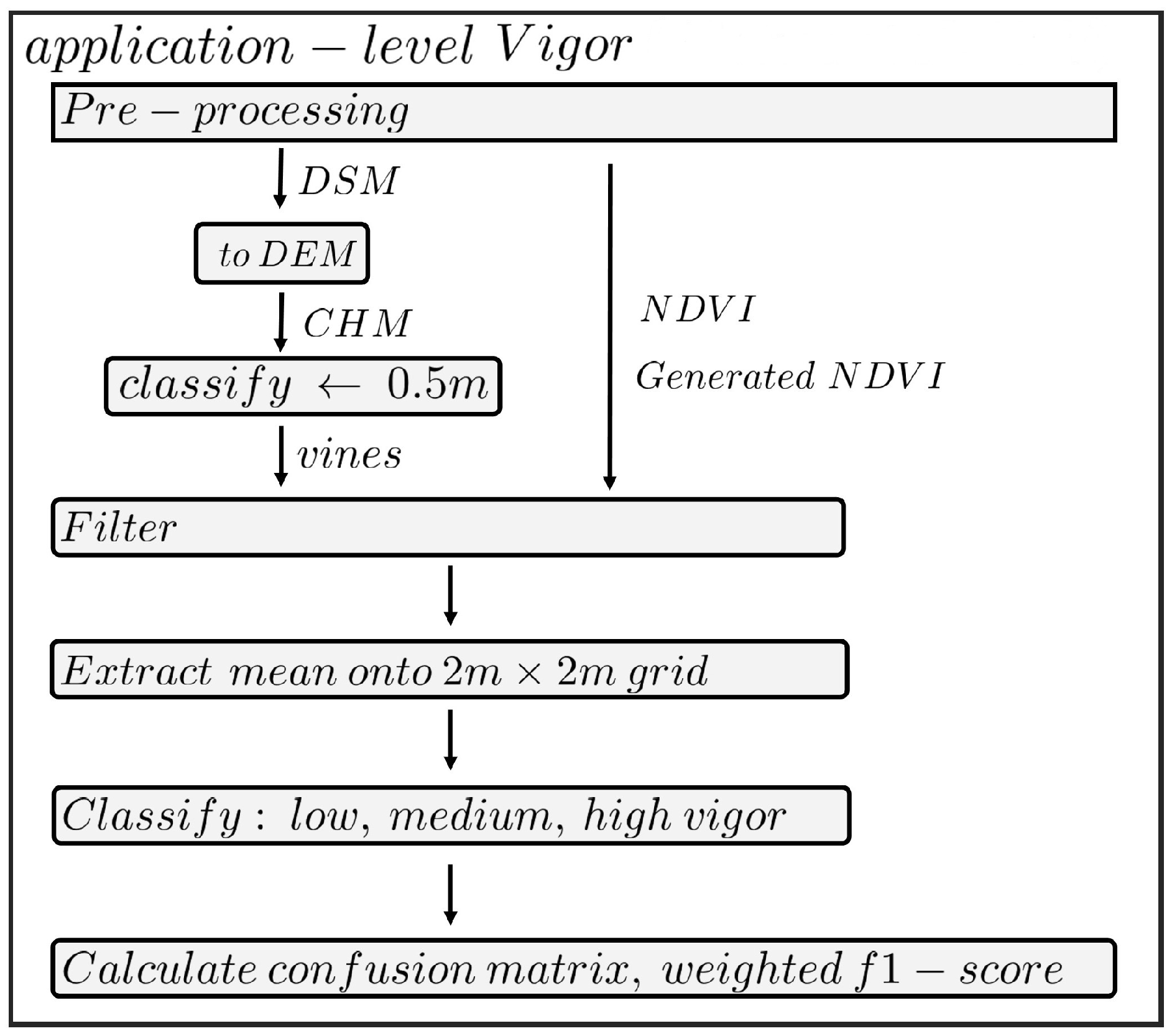
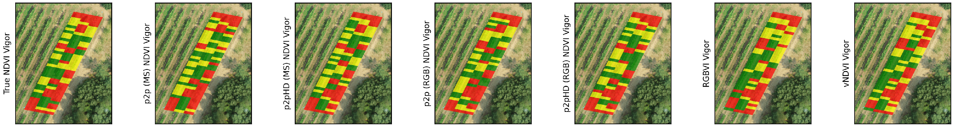
Figure 10.
Processing flowchart for Vigor mapping. In the pre-processing step, the orthomosaic photogrammetric reconstruction, DSM creation and the real and artificial NDVI orthomosaics were generated. The DSM was further processed to acquire a canopy height model (CHM). Then the steps were followed as described in Matese et al. [
4]. Consisting of thresholding to only include canopy rows, mean-extraction onto a 2-by-2-meter grid and classifying the values into tertiles.
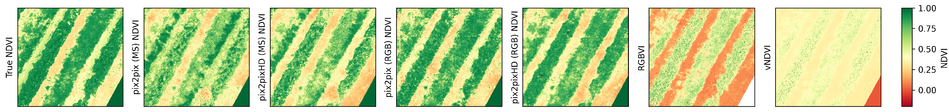
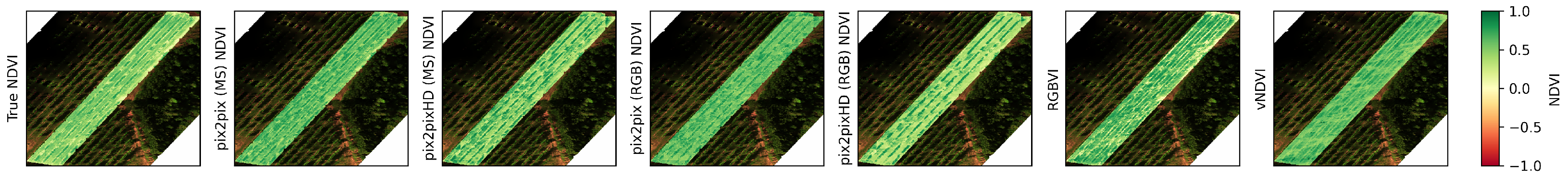
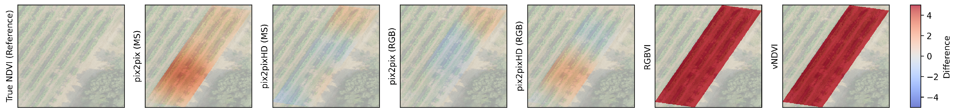
Figure 11.
btg2021 zoomed in. VI color range from (−0.2, 1) to enhance the differences between the images. Green is vegetation, whereas orange is the bare soil, yellow colors indicate grass. The NDVI and generated NDVI maps show a high similarity across both canopy and in-between rows. the RGBVI map has lower values for the bare soil. vNDVI has a lower range of values altogether.
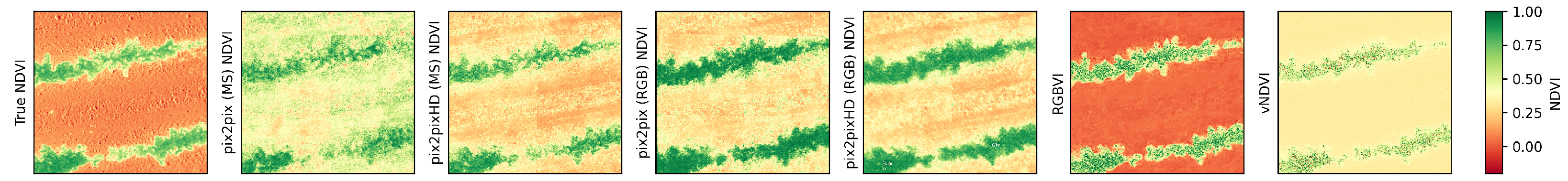
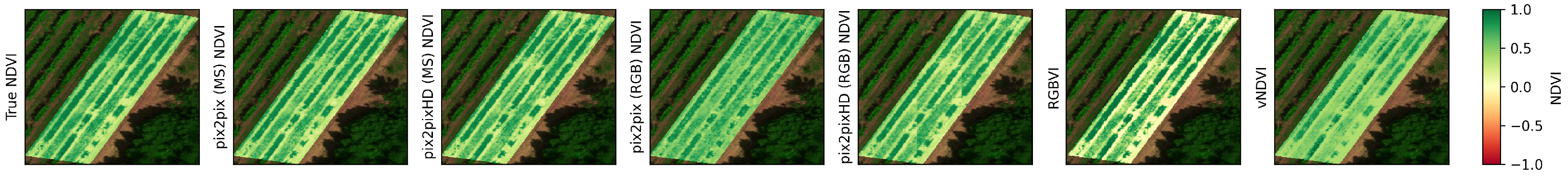
Figure 12.
btg2022ms zoomed in, VI values colored from (−0.2, 1) to enhance the differences between the images. Green is vegetation, whereas orange is the bare soil, yellow colors indicate grass. The NDVI map indicates minimal bare soil, the Pix2Pix maps show less intensity in the canopy vegetation and less grass between rows, RGBVI indicates lower values overall. Pix2Pix has slightly higher values for canopy compared to Pix2PixHD.
Figure 13.
btg2022rgb zoomed in, VI values colored from (−0.2, 1) to enhance the differences between the images. Green is vegetation, whereas orange is the bare soil, yellow colors indicate grass. The NDVI map indicates minimal bare soil, the Pix2Pix maps show less intensity in the canopy vegetation and less grass between rows, and RGBVI indicates lower values overall. Pix2Pix has slightly higher values for canopy compared to Pix2PixHD.
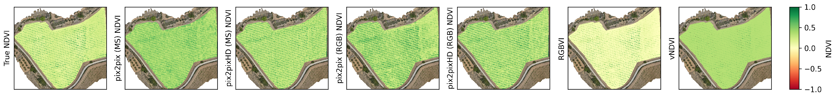
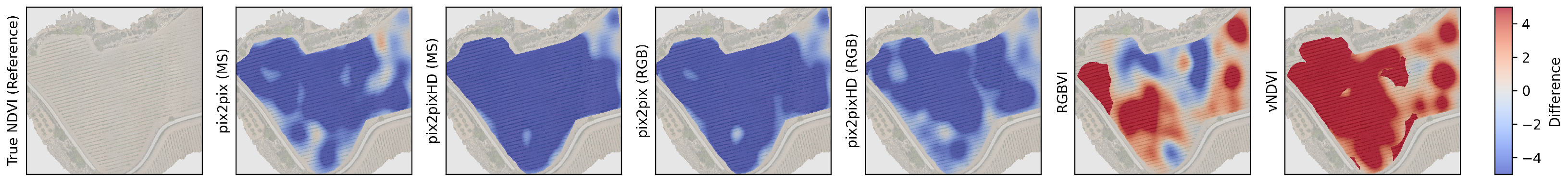
Figure 14.
can2023 zoomed in on tractor tracks, VI color range from (−0.2, 1) to enhance the differences between the images. Green is vegetation, whereas orange is the bare soil, yellow colors indicate grass. The NDVI and RGBVI maps indicate a pattern of tractor tracks and canopy vegetation, Pix2Pix shows more vegetation over the image and hard boundaries between reconstructed chips. Pix2PixHD shows less vegetation than Pix2Pix, although more than the true NDVI image.
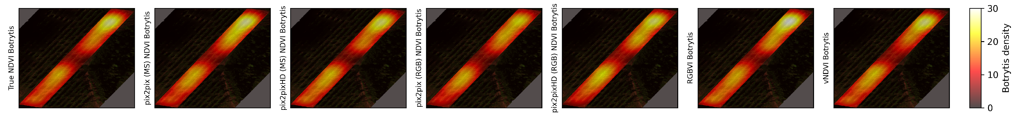
Figure 15.
btg2021 Botrytis bunch rot risk (BBR) heatmap outputs using the different vegetation maps as input.
Figure 15.
btg2021 Botrytis bunch rot risk (BBR) heatmap outputs using the different vegetation maps as input.
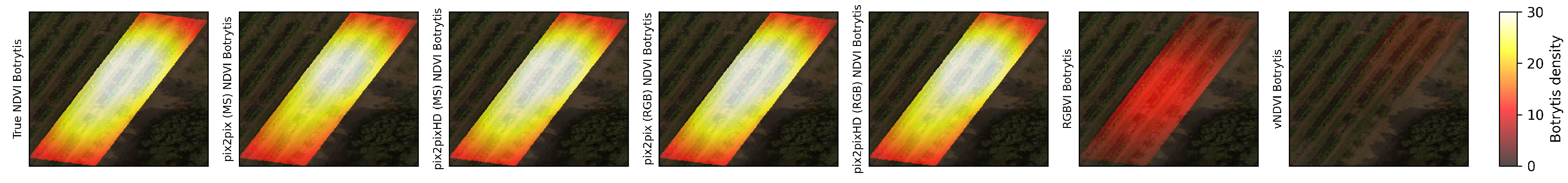
Figure 16.
btg2022ms Botrytis bunch rot risk (BBR) heatmap outputs using the different vegetation maps as input.
Figure 16.
btg2022ms Botrytis bunch rot risk (BBR) heatmap outputs using the different vegetation maps as input.
Figure 17.
btg2022rgb Botrytis bunch rot risk (BBR) heatmap outputs using the different vegetation maps as input.
Figure 17.
btg2022rgb Botrytis bunch rot risk (BBR) heatmap outputs using the different vegetation maps as input.
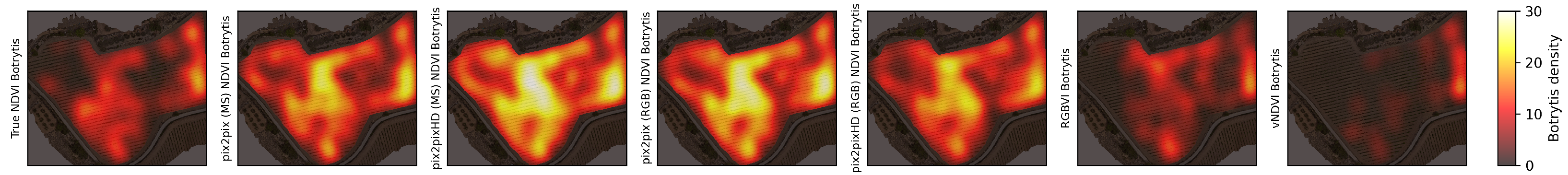
Figure 18.
can2023 Botrytis bunch rot risk (BBR) heatmap outputs using the different vegetation maps as input. There is a high similarity between all the BBR outputs. With the largest difference in risk being shown in the top-left section of the vineyard. In this section, by using the Pix2Pix generated NDVI, the BBR model shows distinct hotspots, Pix2PixHD closely represents the real NDVI map, and RGBVI underestimates the risk, in comparison to using the true NDVI map.
Table 1.
Overview of the employed datasets: btg2021, btg2022 and can2023. WGS84 refers to the coordinates in WGS84 format. doi is the open-access URL to the dataset. AOP is the Area of Appelation of the vineyard.
Table 1.
Overview of the employed datasets: btg2021, btg2022 and can2023. WGS84 refers to the coordinates in WGS84 format. doi is the open-access URL to the dataset. AOP is the Area of Appelation of the vineyard.
| Description | btg | can2023 |
|---|
| Location | Bodegas Terras Gauda, Spain | Canyelles, Spain |
| Date | 16 September 2021
12 July 2022 | 9 June 2023 |
| WGS84 | −8.791, 41.936 | 1.878, 41.319 |
| doi | 2021: 10.5281/zenodo.7383601 [39] | 10.5281/zenodo.8220182 [36] |
| Species | Vitis Vinifera Loureiro | Vitis Vinifera Xarel·lo |
| AOP | Rias Baixas | Penedès |
| Sensor | MicaSense Rededge
MicaSense Altum-PT,
Phantom 4-RTK digital camera | DJI Mavic 3M
Multispectral and digital sensor |
| UAV model | 2021: DJI Matrice M210-RTK
2022: DJI Matrice M300-RTK,
DJI Phantom 4-RTK | DJI Mavic 3M |
| Flight height | 15 m | 10 m |
| Pixel size (cm) | 2021: 1.67
2022: 1.41 | 0.94 |
Table 2.
Training overview for the selected chip sizes. The table summarizes the number of training chips, total training pixels, and epoch time for each model configuration. These numbers are identical for both the MS and RGB subsets.
Table 2.
Training overview for the selected chip sizes. The table summarizes the number of training chips, total training pixels, and epoch time for each model configuration. These numbers are identical for both the MS and RGB subsets.
| Model | Train/Validation/Test Chips | Total Training Pixels | Epoch Time (s) |
|---|
| 1053/110/60 | 69,009,408 | 200 |
| (HD) | 333/37/20 | 87,293,952 | 240 |
Table 3.
Pixel-level R-squared values for all models and datasets. Bold values indicate the best scoring model.
Table 3.
Pixel-level R-squared values for all models and datasets. Bold values indicate the best scoring model.
| Dataset | Pix2Pix (MS) | Pix2PixHD (MS) | Pix2Pix (RGB) | Pix2PixHD (RGB) | RGBVI | vNDVI |
|---|
| btg2021 | 0.103 * | 0.281 * | −0.460 * | 0.049 * | 0.199 * | 0.201 * |
| btg2022ms | 0.837 * | 0.825 * | 0.388 * | 0.479 * | 0.233 * | 0.704 * |
| btg2022rgb | 0.397 * | 0.257 * | 0.637 * | 0.617 * | −1.506 * | −0.683 * |
| can2023 | −0.823 * | −0.021 * | −0.335 * | −0.102 | −0.229 * | −0.142 * |
Table 4.
Pixel-level MSE values for all models and datasets. Bold values indicate the best scoring model.
Table 4.
Pixel-level MSE values for all models and datasets. Bold values indicate the best scoring model.
| Dataset | Pix2Pix (MS) | Pix2PixHD (MS) | Pix2Pix (RGB) | Pix2PixHD (RGB) | RGBVI | vNDVI |
|---|
| btg2021 | 0.037 * | 0.029 * | 0.060 * | 0.039 * | 0.033 * | 0.032 * |
| btg2022ms | 0.009 * | 0.10 * | 0.034 * | 0.029 * | 0.043 * | 0.016 * |
| btg2022rgb | 0.034 * | 0.041 * | 0.020 * | 0.021 * | 0.139 * | 0.094 * |
| can2023 | 0.050 * | 0.028 * | 0.037 * | 0.030 * | 0.033 * | 0.031 * |
Table 5.
Structural Similarity values for all models and datasets. Bold values indicate the best scoring model.
Table 5.
Structural Similarity values for all models and datasets. Bold values indicate the best scoring model.
| Dataset | Pix2Pix (MS) | Pix2PixHD (MS) | Pix2Pix (RGB) | Pix2PixHD (RGB) | RGBVI | vNDVI |
|---|
| btg2021 | 0.453 * | −0.076 * | 0.258 * | 0.059 * | 0.677 * | 0.596 * |
| btg2022ms | 0.707 * | −0.044 * | 0.378 * | 0.139 * | 0.692 * | 0.746 * |
| btg2022rgb | 0.412 * | −0.113 * | 0.478 * | 0.109 * | 0.391 * | 0.514 * |
| can2023 | 0.468 * | −0.103 * | 0.519 * | 0.078 * | 0.655 * | 0.676 * |
Table 6.
Peak signal-to-noise ratiovalues for all models and datasets. Bold values indicate the best scoring model.
Table 6.
Peak signal-to-noise ratiovalues for all models and datasets. Bold values indicate the best scoring model.
| Dataset | Pix2Pix (MS) | Pix2PixHD (MS) | Pix2Pix (RGB) | Pix2PixHD (RGB) | RGBVI | vNDVI |
|---|
| btg2021 | 20.557 * | 3.949 * | 18.507 * | 4.577 * | 21.167 * | 17.838 * |
| btg2022ms | 26.625 * | 4.638 * | 20.624 * | 4.865 * | 19.809 * | 19.557 * |
| btg2022rgb | 21.057 * | 9.521 * | 23.176 * | 9.260 * | 14.787 * | 17.286 * |
| can2023 | 19.008 * | 11.786 * | 20.628 * | 11.559 * | 21.317 * | 20.234 * |
Table 7.
Botrytis bunch rot R-squared values for all models and datasets. Bold values indicate the best scoring model on the dataset.
Table 7.
Botrytis bunch rot R-squared values for all models and datasets. Bold values indicate the best scoring model on the dataset.
| Dataset | Pix2Pix (MS) | Pix2PixHD (MS) | Pix2Pix (RGB) | Pix2PixHD (RGB) | RGBVI | vNDVI |
|---|
| btg2021 | 0.944 * | 0.974 * | 0.874 * | 0.856 * | 0.942 * | 0.950 * |
| btg2022ms | 0.911 * | 0.917 * | 0.992 * | 0.993 * | 0.857 * | 0.971 * |
| btg2022rgb | 0.907 * | 0.992 * | 0.992 | 0.982 * | −5.788 * | −16.906 * |
| can2023 | −1.589 * | −5.752 * | −4.120 * | −1.431 * | 0.213 * | −1.277 * |
Table 8.
Botrytis bunch rot MSE values for all models and datasets. Bold values indicate the best scoring model on the dataset.
Table 8.
Botrytis bunch rot MSE values for all models and datasets. Bold values indicate the best scoring model on the dataset.
| Dataset | Pix2Pix (MS) | Pix2PixHD (MS) | Pix2Pix (RGB) | Pix2PixHD (RGB) | RGBVI | vNDVI |
|---|
| btg2021 | 1.464 * | 0.671 * | 3.274 * | 3.761 | 1.500 * | 1.297 * |
| btg2022ms | 3.717 * | 3.466 * | 0.339 * | 0.277 * | 5.976 * | 1.221 * |
| btg2022rgb | 3.899 * | 0.315 * | 0.347 * | 0.751 * | 283.954 * | 601.860 * |
| can2023 | 41.476 * | 108.172 * | 82.017 | 38.938 * | 12.636 * | 31.825 * |
Table 9.
Vigor mapping weighted F1-scores for all models and datasets.
Table 9.
Vigor mapping weighted F1-scores for all models and datasets.
| Dataset | Pix2Pix (MS) | Pix2PixHD (MS) | Pix2Pix (RGB) | Pix2PixHD (RGB) | RGBVI | vNDVI |
|---|
| btg2021 | 0.805 (0.009) | 0.740 (0.025) | 0.544 (0.125) | 0.555 (0.138) | 0.847
(0.005) | 0.786 (0.014) |
| btg2022ms | 0.789 (0.019) | 0.807 (0.011) | 0.570 (0.094) | 0.605 (0.063) | 0.904
(0.002) | 0.860 (0.006) |
| btg2022rgb | 0.728 (0.033) | 0.789
(0.019) | 0.782 (0.016) | 0.771 (0.026) | 0.693 (0.028) | 0.649 (0.039) |
| can2023 | 0.660 (0.052) | 0.483 (0.134) | 0.653 (0.059) | 0.583 (0.067) | 0.661 (0.054) | 0.661
(0.051) |
Table 10.
Domain Shift Scenarios within UAV Remote Sensing.
Table 10.
Domain Shift Scenarios within UAV Remote Sensing.
| Research Direction | Description and Examples |
|---|
| Sensor Modality | Explore domain shifts between different sensor modalities (e.g., multispectral, hyperspectral, RGB, thermal). |
| Intra Sensor Modality Variability | Study style transfer within the same sensor type (e.g., different multispectral sensors or varying hyperspectral band configurations) to handle sensor-specific color calibration, sensor aging effects, and manufacturer differences. |
| Subject Matter | Examine how models can generalize to different applications such as fruit detection, plant health assessment, soil moisture estimation, and disease detection when trained on one specific target (e.g., detecting disease on grapes) and applied to another (e.g., detecting disease on apples). |
| Lighting and Atmospheric Conditions | Investigate how models cope with varying illumination (e.g., high sun angles, diffuse light, cloudy conditions), seasonal sun position shifts, or atmospheric scattering. |
| Geographic and Climatic Variability | Address domain shifts between regions (e.g., vineyards in Spain vs. orchards in California), climates, or soil types. Research focuses on enabling models trained in one locale to generalize to new locations with different environmental conditions. |
| Sensor Viewing Angle | Explore how variations in camera angles, UAV flight patterns, and sensor tilt affect data quality and consistency. |
| Temporal Domain Shifts | Consider changes over time—day-to-day, seasonal, or yearly—to ensure models remain effective despite phenological stages of crops, evolving canopy structures, or changing management practices. |


