
A Machine Learning Algorithm to Convert Geostationary Satellite LST to Air Temperature Using In Situ Measurements: A Case Study in Rome and High-Resolution Spatio-Temporal UHI Analysis


Abstract
1. Introduction
2. Materials and Methods
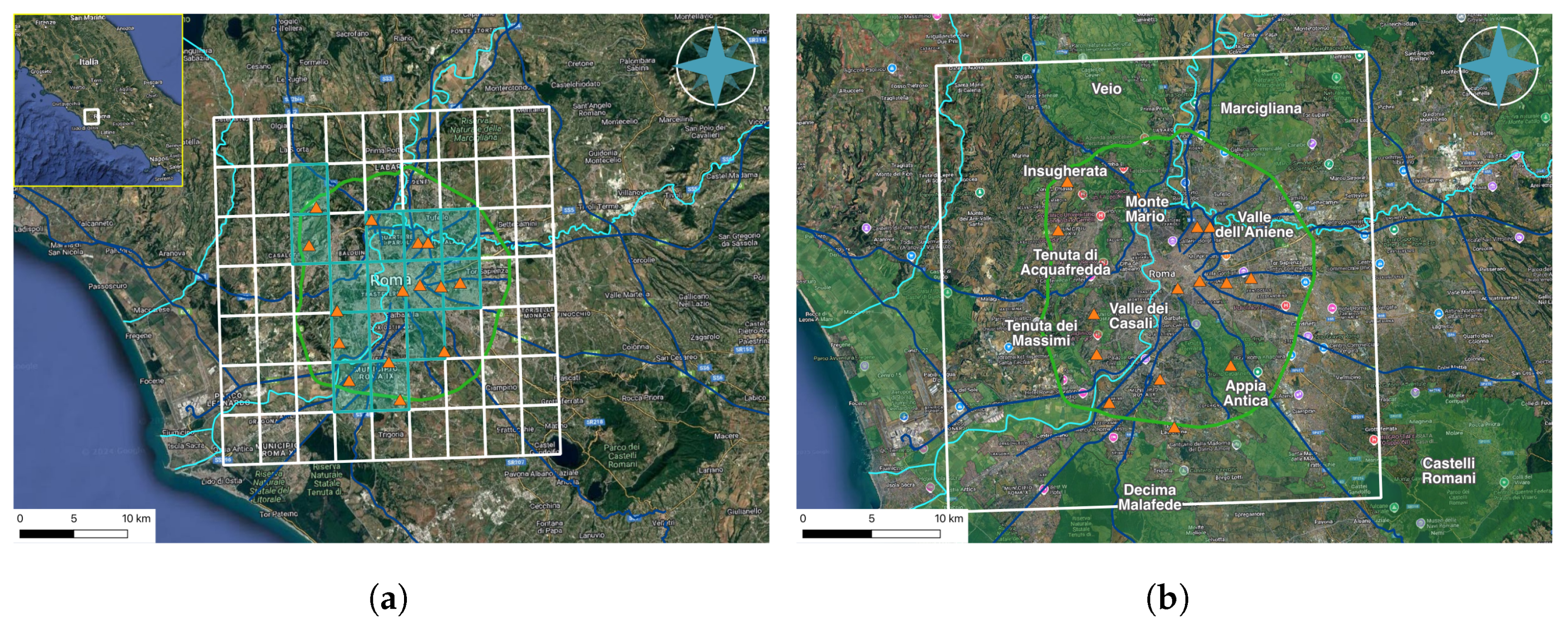
2.1. Study Area
2.2. Conceptualization
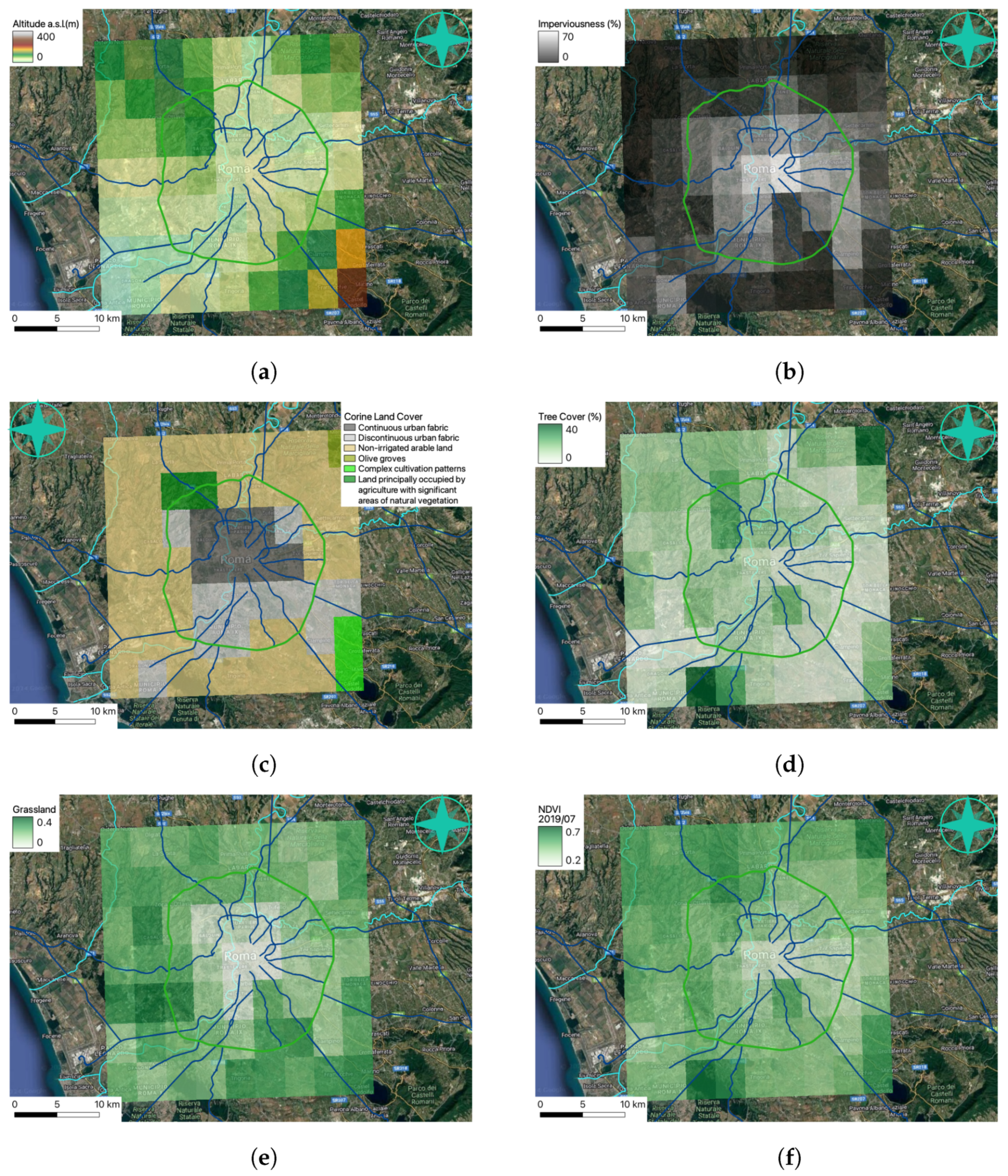
2.3. Input Data
- LST: land surface temperature, produced by the EUMETSAT Satellite Application Facility (SAF) on Land Surface Analysis (LSA), code MLST [LSA-001], measured by the Spinning Enhanced Visible and InfraRed Imager (SEVIRI) instrument mounted on the Meteosat Second Generation (MSG) satellites launched by the European Spatial Agency (ESA). Instead of using the raw SEVIRI data, the operational LST product from the Land Surface Analysis Satellite Applications Facility (LSA SAF) was used (https://landsaf.ipma.pt/en/data/products/land-surface-temperature-and-emissivity/, last accessed on 14 March 2024), in which the pixels containing clouds are masked. The overall accuracy of the LST product is about 2 K [23], and its spatial and temporal resolutions are, respectively, 3 km and 15 min.
- DTM: digital terrain model, i.e., elevation a.s.l. in meters. Data extracted from the EU-DEM product [24], with a spatial resolution of 25 m and an accuracy of ±7 m RMSE. The year of measurement is 2010.
- Imperviousness Density: density of impervious surfaces. It represents the percentage of an area covered by artificially sealed surfaces, such as roads or buildings. It ranges from 0% to 100%, with a resolution of 1%, and is provided with a spatial resolution of 10 m. The year of measurement is 2018.
- Tree Cover Density: represents the percentage presence of trees. Like imperviousness, it ranges from 0% to 100% with a step of 1%, and is provided with a spatial resolution of 10 m. The year of measurement is 2018.
- Corine Land Cover: represents an inventory of land cover and land use, with 44 thematic classes ranging from extensive forest areas to single vineyards. Therefore, it is a discrete dataset based on categories, with a spatial resolution of 100 m, and the year of measurement is 2018.
- Grassland: A binary pan-European product that provides a presence/absence mask of grasslands. Therefore, it can only take two values, 0 or 1, and is provided with a spatial resolution of 10 m, and the year of measurement is 2018.
- NDVI: The normalized difference vegetation index (NDVI) quantifies the presence and health of vegetation cover. The data used here were recorded by the MODIS (Moderate Resolution Imaging Spectroradiometer) instrument aboard the Terra satellite, and are part of the MODIS/Terra Vegetation Indices Monthly L3 Global 1km SIN Grid V006 dataset [25], with spatial and temporal resolutions of 1 km and 1 month, respectively. The value range varies from −0.2 to 1.0, with a resolution of 0.0001. When the value is 0, there is no vegetation, while increasingly positive values indicate increasing vegetation density, peaking at 1.0 for very dense and healthy vegetation. Negative values indicate the presence of water bodies.
- Air temperature: This data is provided by in situ measurements from 15 weather stations, indicated by the orange triangles in Figure 1. These stations are part of the ASTI-Network, established within the framework of the LIFE-ASTI project. The network includes stations from the Meteo Lazio amateur network [26], as well as additional stations installed specifically during the project to cover areas lacking data.
2.4. Setting the Gradient-Boosting Algorithm
2.5. Error Estimation and Hyperparameters
2.6. Calculating UHI Intensity
3. Results
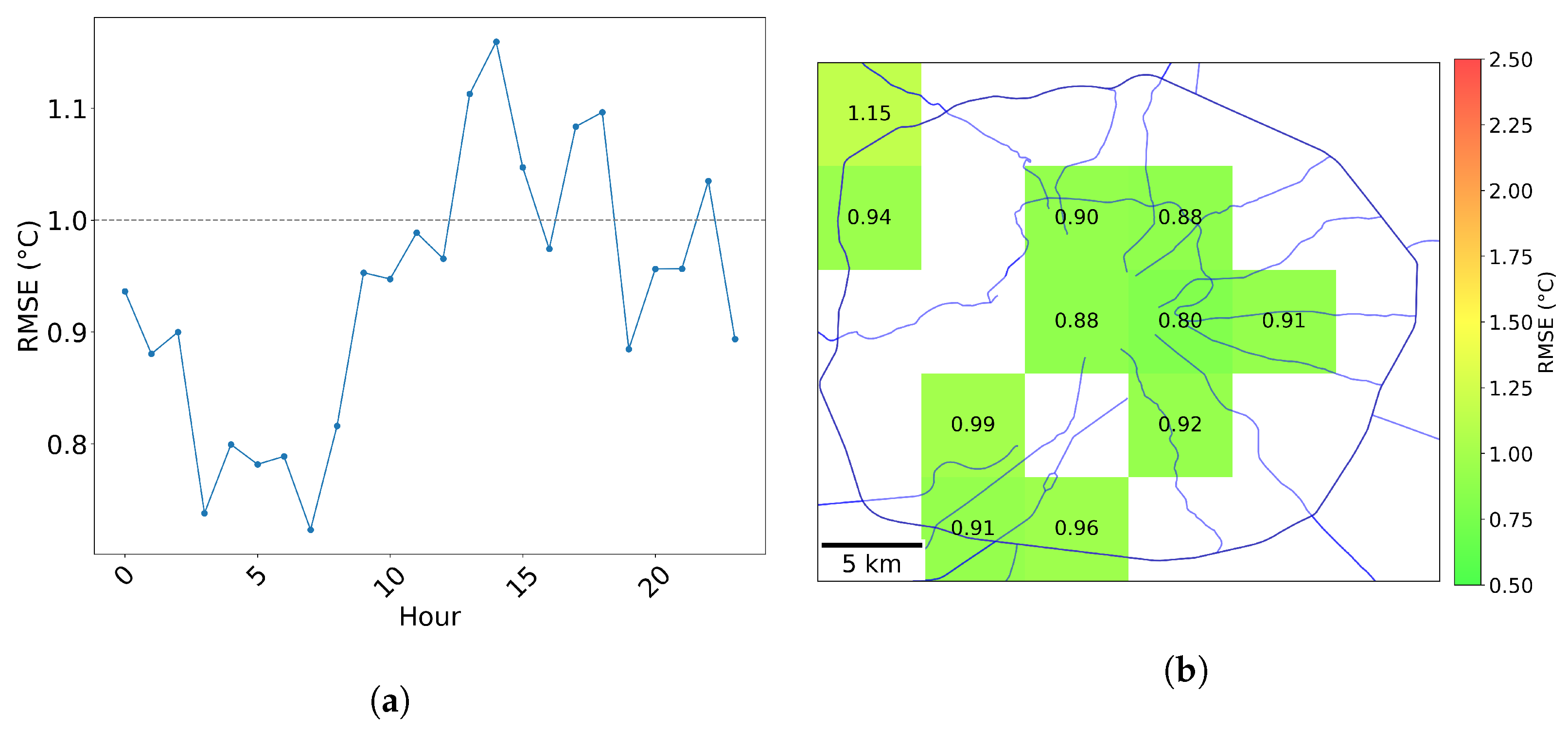
3.1. Error Analysis
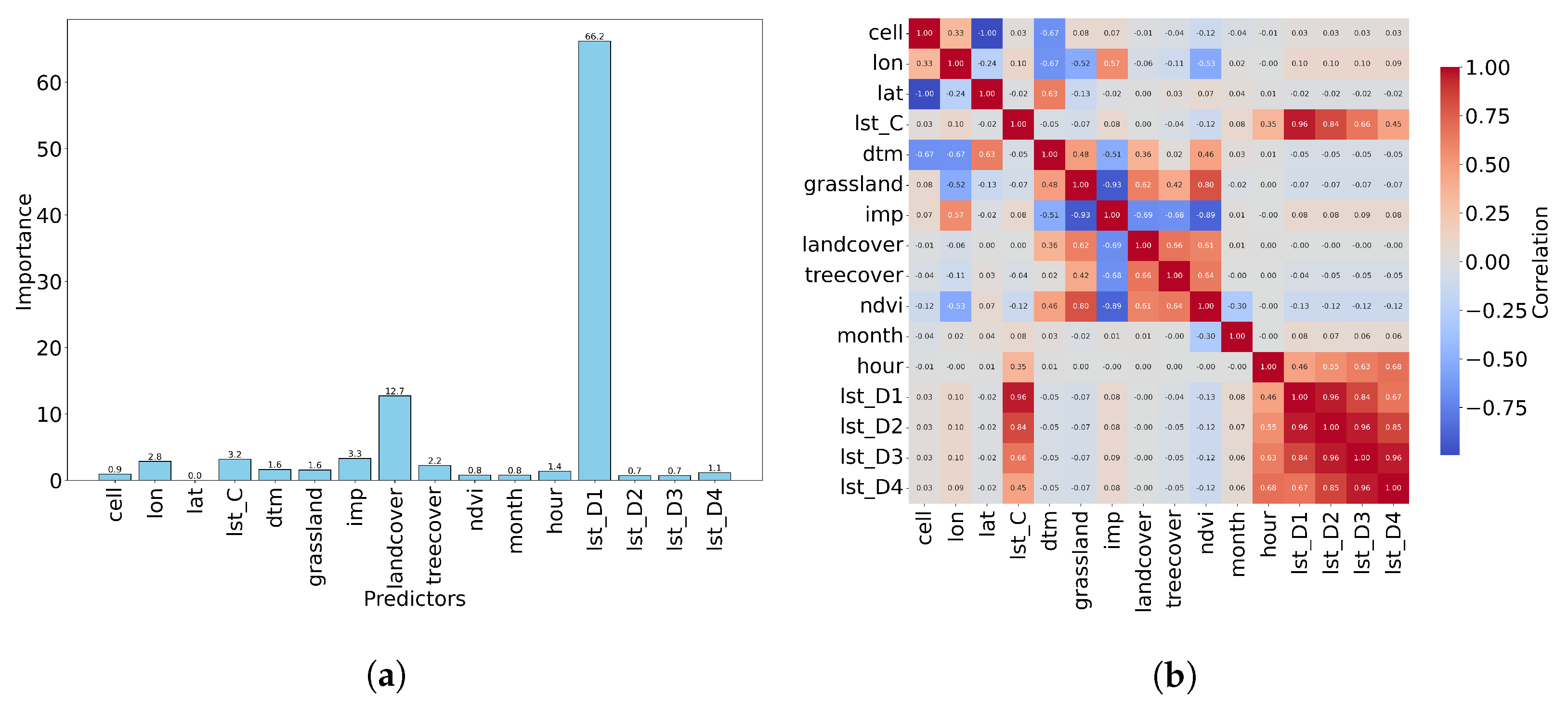
3.2. Predictors Importance and Correlations
3.3. Daily Maximum and Minimum Temperatures
3.4. UHI and SUHI Intensity
3.4.1. UHI
3.4.2. SUHI
4. Discussion
5. Conclusions
Author Contributions
Funding
Data Availability Statement
Acknowledgments
Conflicts of Interest
Abbreviations
| UHI | Canopy Layer Urban Heat Island |
| SUHI | Surface Urban Heat Island |
| LST | Land Surface Temperature |
| IMP | Imperviousness |
| NDVI | Normalized Difference Vegetation Index |
| RMSE | Root of mean squared error |
| a.s.l. | above sea level |
References
- Oke, T.R.; Mills, G.; Christen, A.; Voogt, J.A. Urban Climates; Cambridge University Press: Cambridge, UK, 2017. [Google Scholar] [CrossRef]
- Marinaccio, A.; Scortichini, M.; Gariazzo, C.; Leva, A.; Bonafede, M.; De’ Donato, F.K.; Stafoggia, M. Nationwide epidemiological study for estimating the effect of extreme outdoor temperature on occupational injuries in Italy. Environ. Int. 2019, 133, 105176. [Google Scholar] [CrossRef]
- Ciardini, V.; Argentini, S.; Sozzi, R.; Caporaso, L.; Petenko, I.; Bolignano, A.; Morelli, M.; Melas, D.A. Interconnections of the urban heat island with the spatial and temporal micrometeorological variability in Rome. Urban Clim. 2019, 29, 100493. [Google Scholar] [CrossRef]
- Zhou, D.; Xiao, J.; Bonafoni, S.; Berger, C.; Deilami, K.; Zhou, Y.; Frolking, S.; Yao, R.; Qiao, Z.; Sobrino, J.A. Satellite remote sensing of surface urban heat islands: Progress, challenges, and perspectives. Remote Sens. 2019, 11, 48. [Google Scholar] [CrossRef]
- United Nations, Department of Economic and Social Affairs, Population Division. World Urbanization Prospects: The 2018 Revision, Custom Data Acquired via Website. 2018. Available online: https://population.un.org/wup/assets/WUP2018-Report.pdf (accessed on 22 January 2025).
- Meehl, G.; Tebaldi, C. More Intense, More Frequent, and Longer Lasting Heat Waves in the 21st Century. Science 2004, 305, 994–997. [Google Scholar] [CrossRef]
- Chen, E.; Allen, L., Jr.; Bartholic, J.; Gerber, J. Comparison of winter-nocturnal geostationary satellite infrared-surface temperature with shelter-height temperature in Florida. Remote Sens. Environ. 1983, 13, 313–327. [Google Scholar] [CrossRef]
- Bechtel, B.; Wiesner, S.; Zaksek, K. Estimation of Dense Time Series of Urban Air Temperatures from Multitemporal Geostationary Satellite Data. IEEE J. Sel. Top. Appl. Earth Obs. Remote Sens. 2014, 7, 4129–4137. [Google Scholar] [CrossRef]
- Good, E. Daily minimum and maximum surface air temperatures from geostationary satellite data. J. Geophys. Res. Atmos. 2015, 120, 2306–2324. [Google Scholar] [CrossRef]
- Pichierri, M.; Bonafoni, S.; Biondi, R. Satellite air temperature estimation for monitoring the canopy layer heat island of Milan. Remote Sens. Environ. 2012, 127, 130–138. [Google Scholar] [CrossRef]
- Nieto, H.; Sandholt, I.; Aguado, I.; Chuvieco, E.; Stisen, S. Air Temperature Estimation with MSG-SEVIRI Data: Calibration and Validation of the TVX Algorithm for the Iberian Peninsula. Remote Sens. Environ. 2011, 115, 107–116. [Google Scholar] [CrossRef]
- Wloczyk, C.; Borg, E.; Richter, R.; Miegel, K. Estimation of instantaneous air temperature above vegetation and soil surfaces from Landsat 7 ETM+ data in northern Germany. Int. J. Remote Sens. 2011, 32, 9119–9136. [Google Scholar] [CrossRef]
- Agathangelidis, I.; Cartalis, C.; Santamouris, M. Estimation of Air Temperatures for the Urban Agglomeration of Athens with the Use of Satellite Data. Geoinform. Geostat. Overv. 2016, 4, 2. [Google Scholar] [CrossRef]
- dos Santos, R.S. Estimating spatio-temporal air temperature in London (UK) using machine learning and earth observation satellite data. Int. J. Appl. Earth Obs. Geoinf. 2020, 88, 102066. [Google Scholar] [CrossRef]
- Carrión, D.; Arfer, K.B.; Rush, J.; Dorman, M.; Rowland, S.T.; Kioumourtzoglou, M.A.; Kloog, I.; Just, A.C. A 1-km hourly air-temperature model for 13 northeastern U.S. states using remotely sensed and ground-based measurements. Environ. Res. 2021, 200, 111477. [Google Scholar] [CrossRef]
- Tran, D.P.; Liou, Y.A. Creating a spatially continuous air temperature dataset for Taiwan using thermal remote-sensing data and machine learning algorithms. Ecol. Indic. 2024, 158, 111469. [Google Scholar] [CrossRef]
- Wang, C.; Bi, X.; Luan, Q.; Li, Z. Estimation of Daily and Instantaneous Near-Surface Air Temperature from MODIS Data Using Machine Learning Methods in the Jingjinji Area of China. Remote Sens. 2022, 14, 1916. [Google Scholar] [CrossRef]
- Cecilia, A.; Casasanta, G.; Petenko, I.; Conidi, A.; Argentini, S. Measuring the urban heat island of Rome through a dense weather station network and remote sensing imperviousness data. Urban Clim. 2022, 47, 101355. [Google Scholar] [CrossRef]
- Italian National Institute of Statistics (ISTAT). 2020. Available online: https://www.istat.it (accessed on 22 January 2025).
- Sozzi, R.; Casasanta, G.; Cecilia, A.; Argentini, S.; Ciardini, V.; Finardi, S.; Petenko, I. Surface and aerodynamic parameters estimation for urban and rural areas. Atmosphere 2020, 11, 147. [Google Scholar] [CrossRef]
- Köppen, W. Das geographische System der Klimate. Handb. Klimatol. 1936, 1. Available online: https://koeppen-geiger.vu-wien.ac.at/pdf/Koppen_1936.pdf (accessed on 22 January 2025).
- Kottek, M.; Grieser, J.; Beck, C.; Rudolf, B.; Rubel, F. World Map of the Köppen-Geiger Climate Classification Updated. Meteorol. Z. 2006, 15, 259–263. [Google Scholar] [CrossRef] [PubMed]
- Trigo, I.F.; Monteiro, I.T.; Olesen, F.; Kabsch, E. An assessment of remotely sensed land surface temperature. J. Geophys. Res. 2008, 113, D17108. [Google Scholar] [CrossRef]
- Copernicus EU. EU-DEM; Ultimo Accesso: Fresno, CA, USA, 15 March 2024. [Google Scholar]
- Didan, K. MODIS/Terra Vegetation Indices Monthly L3 Global 1km SIN Grid V061. 2021. Available online: https://doi.org/10.5067/MODIS/MOD13A3.061 (accessed on 15 March 2024). [CrossRef]
- Meteo Lazio, a Private Meteorological Center for Lazio Region, Which Mainly Deals with Monitoring Through Its Own Network of Meteorological Stations. Available online: https://www.meteoregionelazio.it/ (accessed on 22 January 2025).
- Copernicus EU. Land Monitoring Service; Ultimo Accesso: Fresno, CA, USA, 15 March 2024. [Google Scholar]
- Schatz, J.; Kucharik, C.J. Urban Climate Effects on Extreme Temperatures in Madison, Wisconsin, USA. Environ. Res. Lett. 2015, 10, 094024. [Google Scholar] [CrossRef]
- Sismanidis, P.; Keramitsoglou, I.; Kiranoudis, C. Diurnal analysis of surface Urban Heat Island using spatially enhanced satellite derived LST data. In Proceedings of the 2015 Joint Urban Remote Sensing Event (JURSE), Lausanne, Switzerland, 30 March–1 April 2015. [Google Scholar] [CrossRef]
Disclaimer/Publisher’s Note: The statements, opinions and data contained in all publications are solely those of the individual author(s) and contributor(s) and not of MDPI and/or the editor(s). MDPI and/or the editor(s) disclaim responsibility for any injury to people or property resulting from any ideas, methods, instructions or products referred to in the content. |
© 2025 by the authors. Licensee MDPI, Basel, Switzerland. This article is an open access article distributed under the terms and conditions of the Creative Commons Attribution (CC BY) license (https://creativecommons.org/licenses/by/4.0/).
Share and Cite
Cecilia, A.; Casasanta, G.; Petenko, I.; Argentini, S. A Machine Learning Algorithm to Convert Geostationary Satellite LST to Air Temperature Using In Situ Measurements: A Case Study in Rome and High-Resolution Spatio-Temporal UHI Analysis. Remote Sens. 2025, 17, 468. https://doi.org/10.3390/rs17030468
Cecilia A, Casasanta G, Petenko I, Argentini S. A Machine Learning Algorithm to Convert Geostationary Satellite LST to Air Temperature Using In Situ Measurements: A Case Study in Rome and High-Resolution Spatio-Temporal UHI Analysis. Remote Sensing. 2025; 17(3):468. https://doi.org/10.3390/rs17030468
Chicago/Turabian StyleCecilia, Andrea, Giampietro Casasanta, Igor Petenko, and Stefania Argentini. 2025. "A Machine Learning Algorithm to Convert Geostationary Satellite LST to Air Temperature Using In Situ Measurements: A Case Study in Rome and High-Resolution Spatio-Temporal UHI Analysis" Remote Sensing 17, no. 3: 468. https://doi.org/10.3390/rs17030468
APA StyleCecilia, A., Casasanta, G., Petenko, I., & Argentini, S. (2025). A Machine Learning Algorithm to Convert Geostationary Satellite LST to Air Temperature Using In Situ Measurements: A Case Study in Rome and High-Resolution Spatio-Temporal UHI Analysis. Remote Sensing, 17(3), 468. https://doi.org/10.3390/rs17030468