
A Pixel-Based Machine Learning Atmospheric Correction for PeruSAT-1 Imagery


Abstract
1. Introduction
2. Materials and Methods
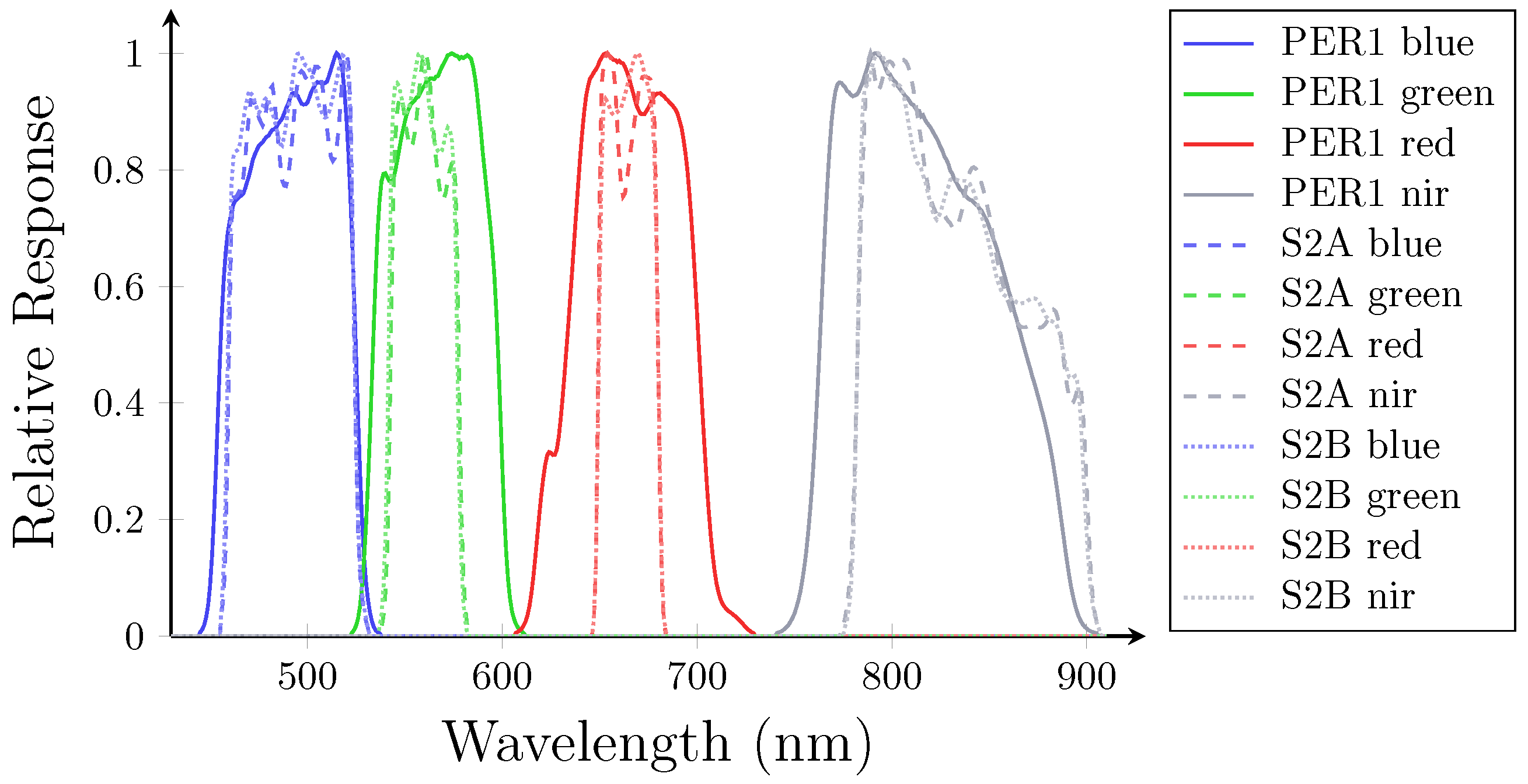
2.1. Satellite and Data Description
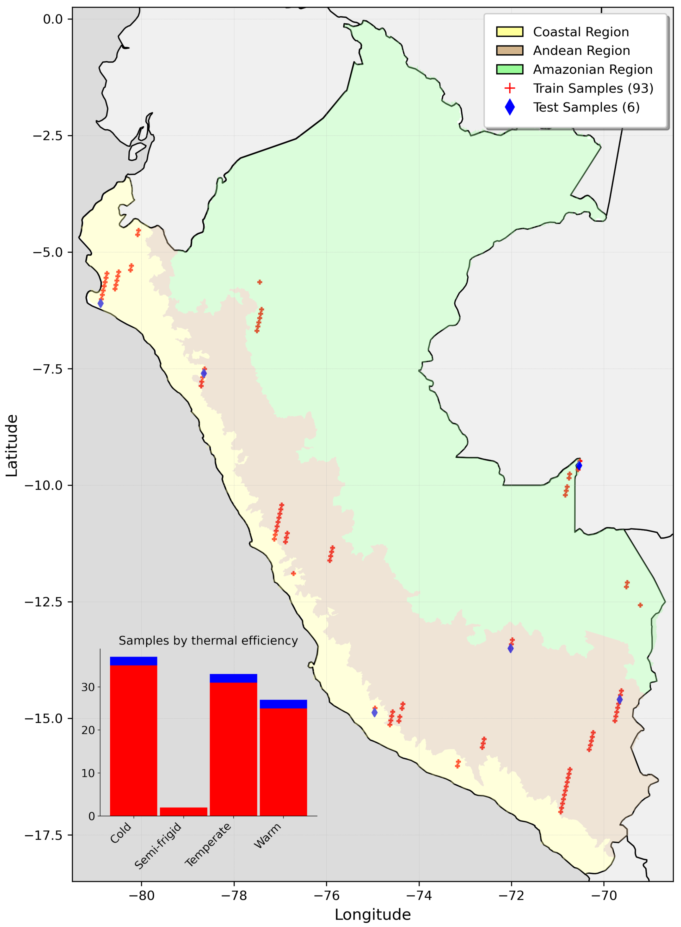
2.2. Dataset Creation
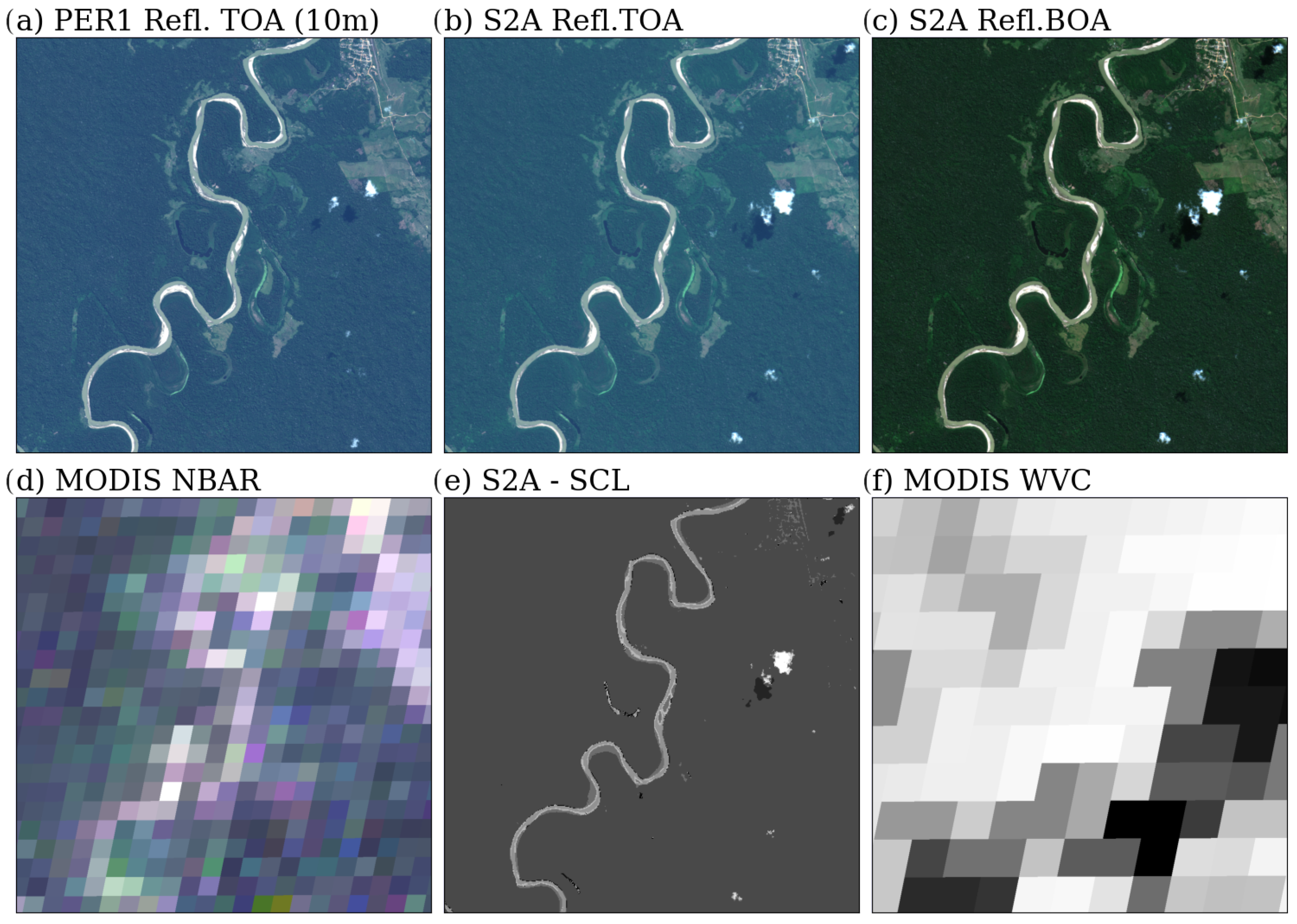
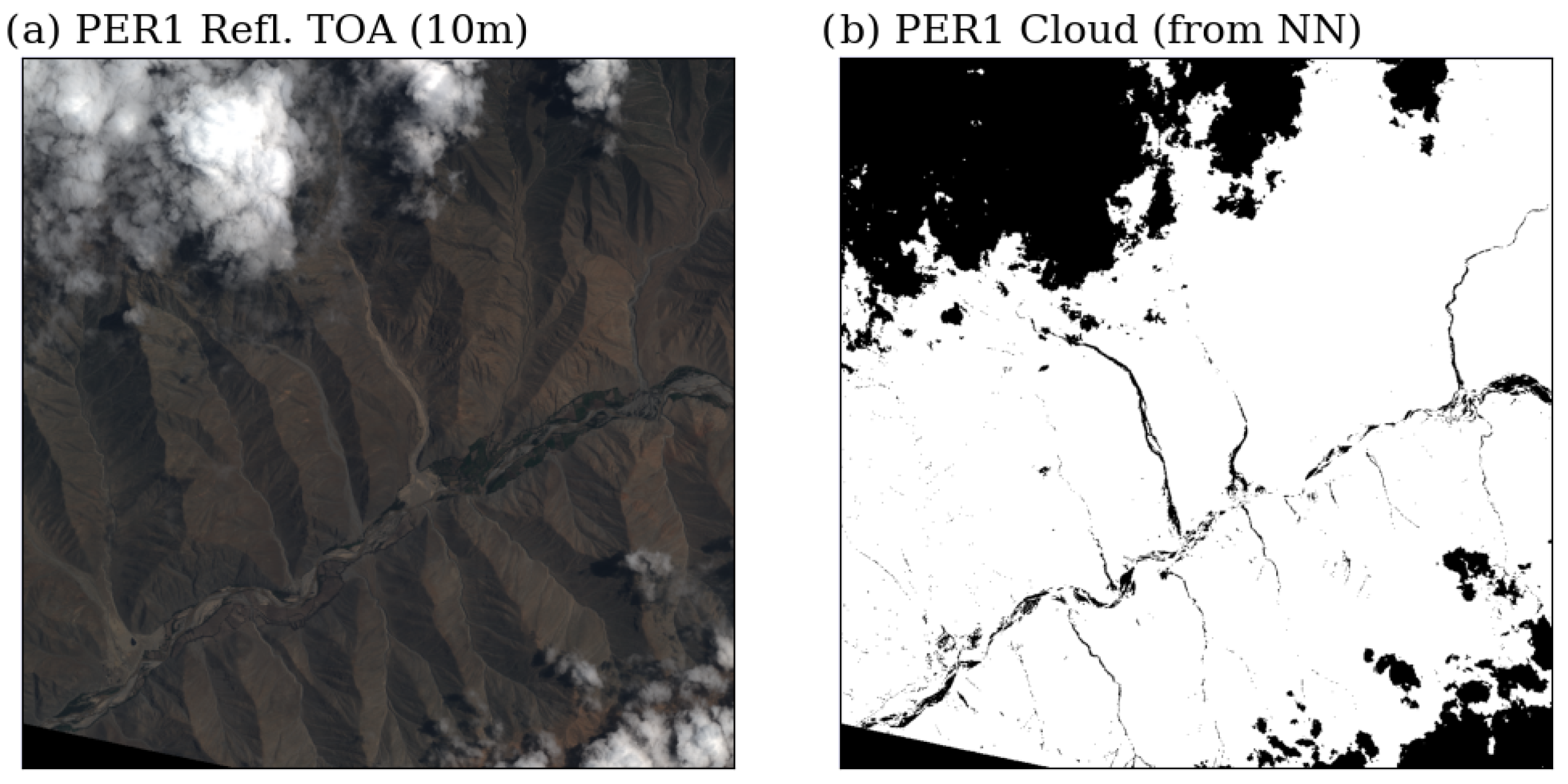
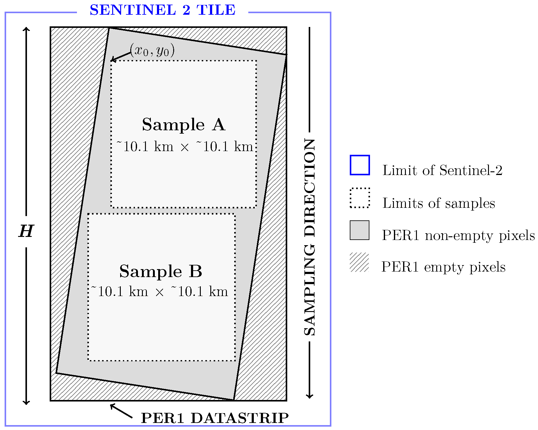
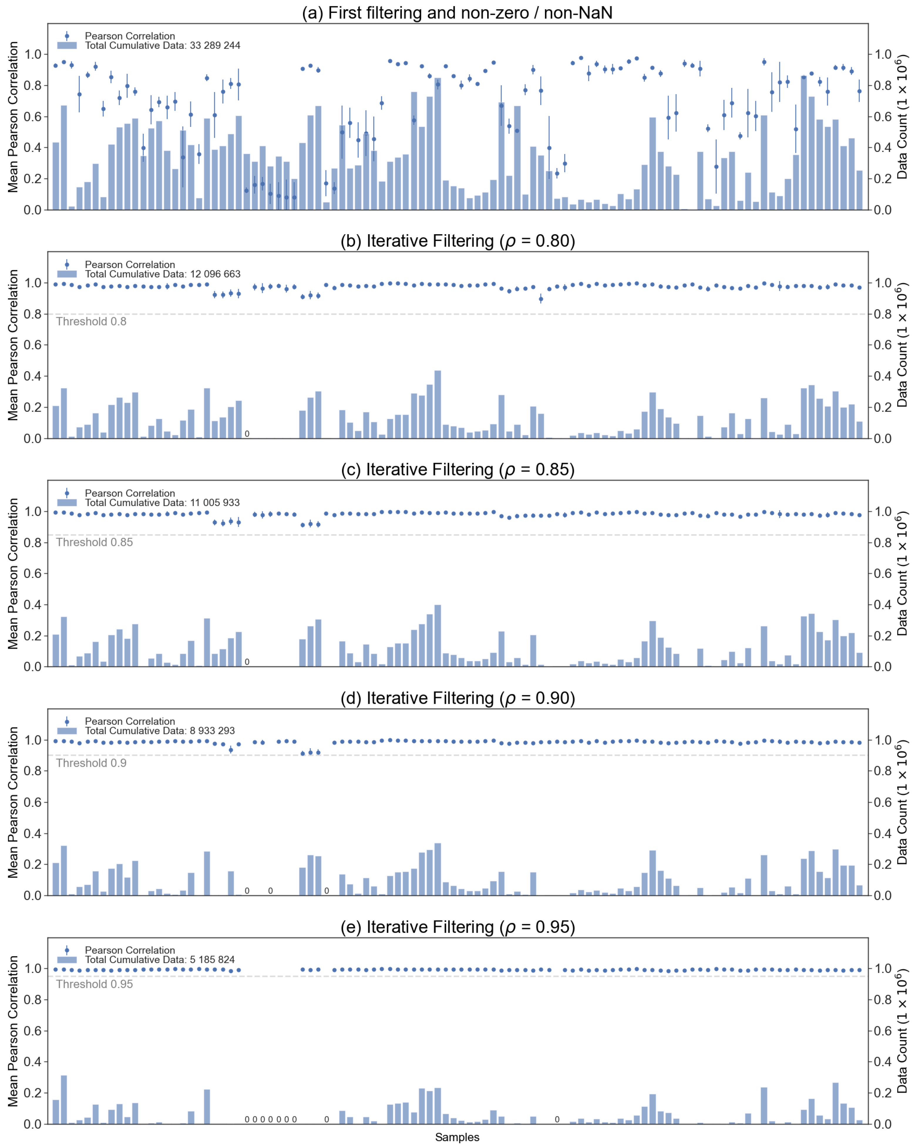
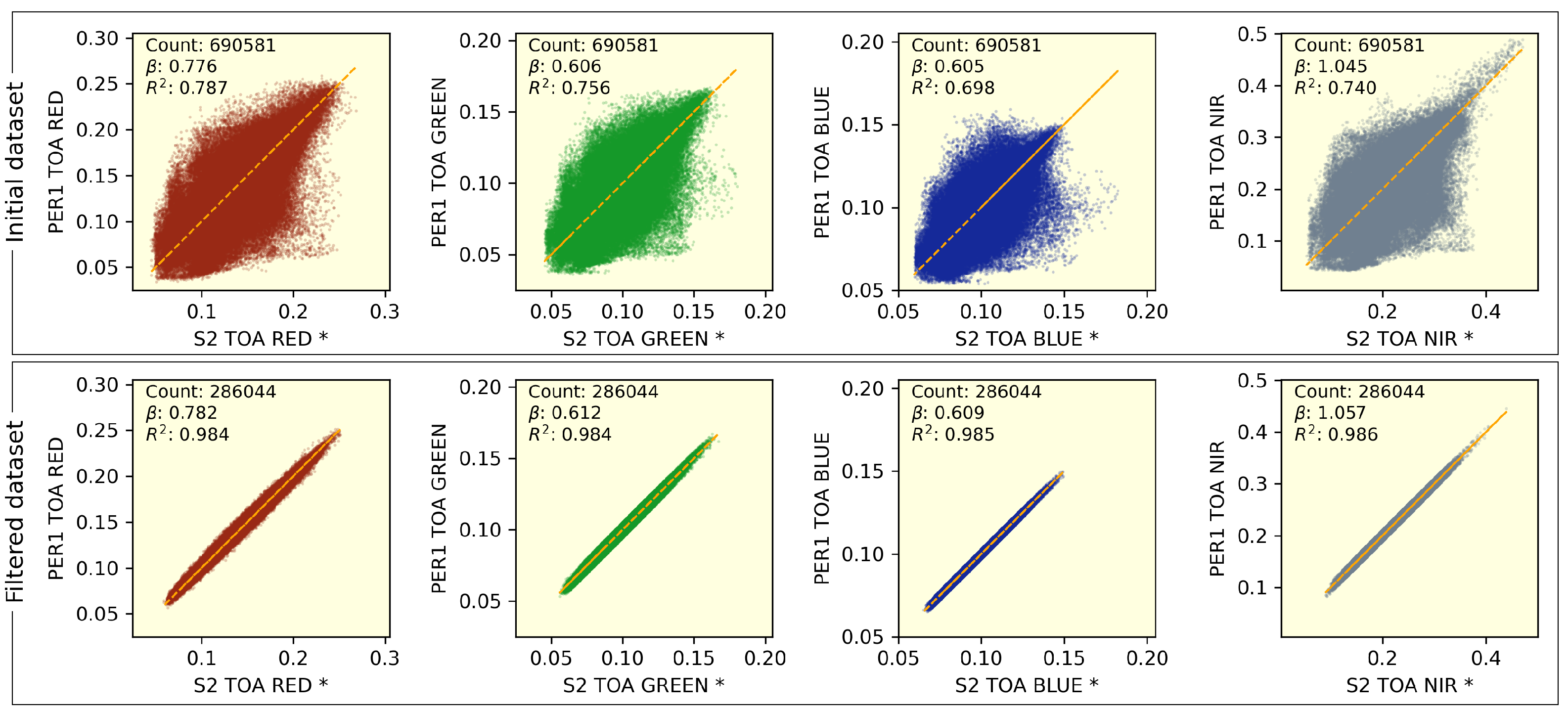
2.3. Dataset Preprocessing
2.4. Machine Learning Experiments
2.4.1. Multiple Linear Regression Approach
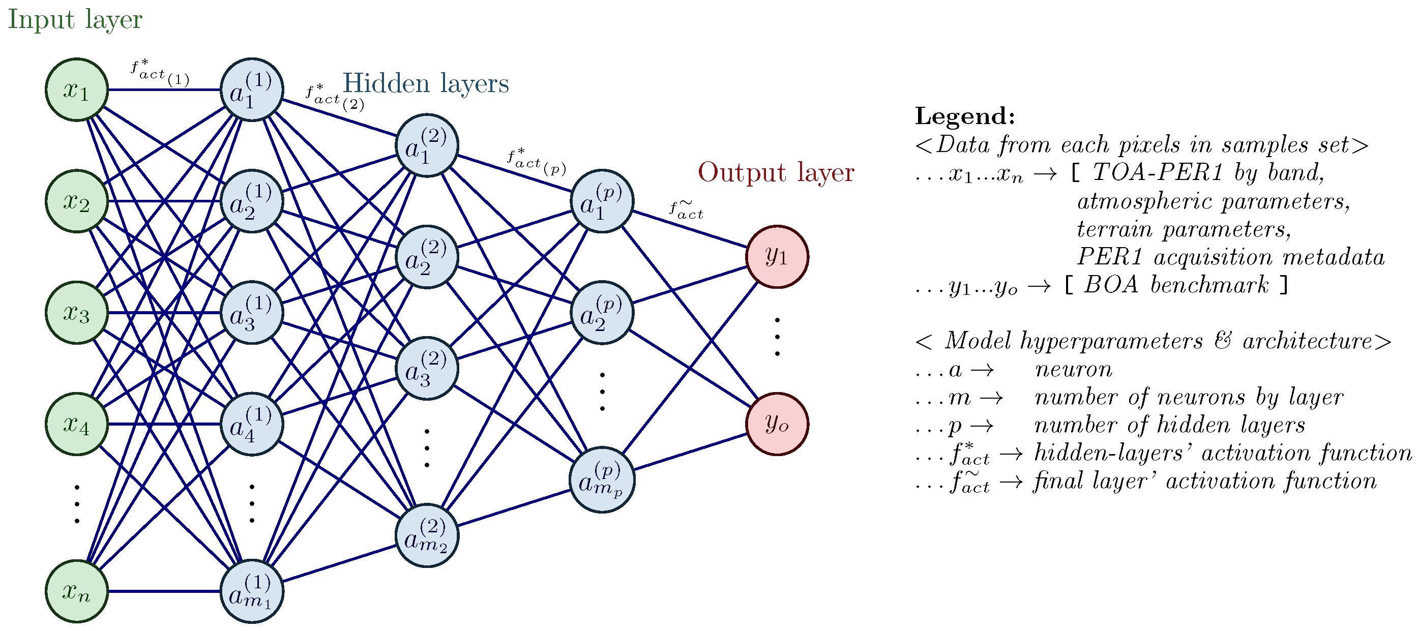
2.4.2. Feedforward Neural Network Approach
3. Results
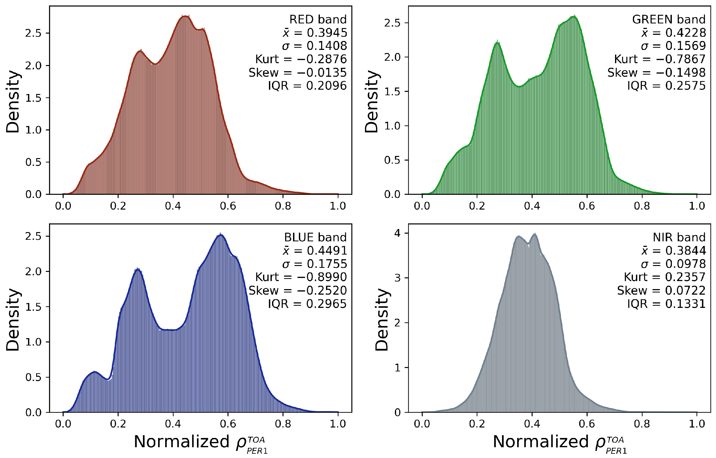
3.1. Final Dataset
3.2. Machine Learning Experiments Results
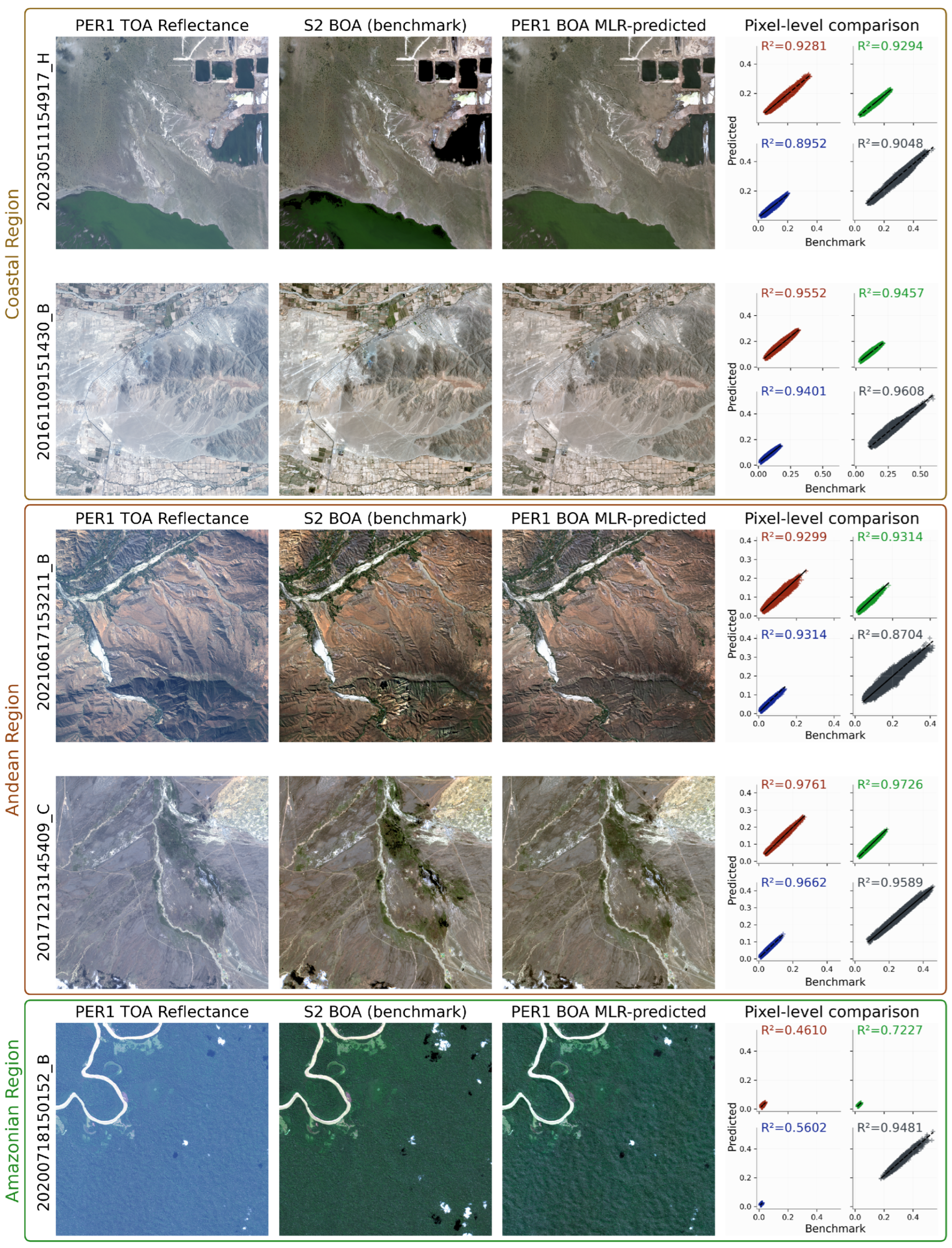
3.2.1. Multiple Linear Regression Approach
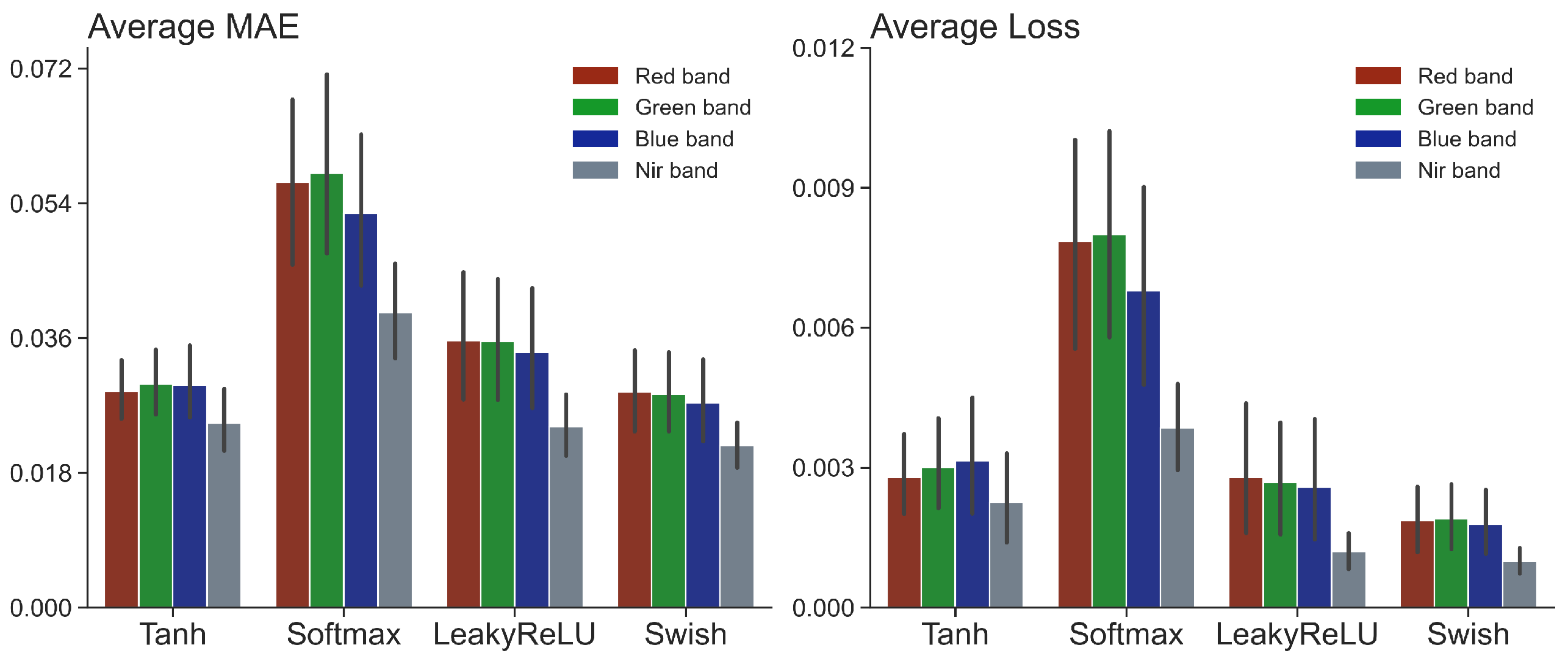
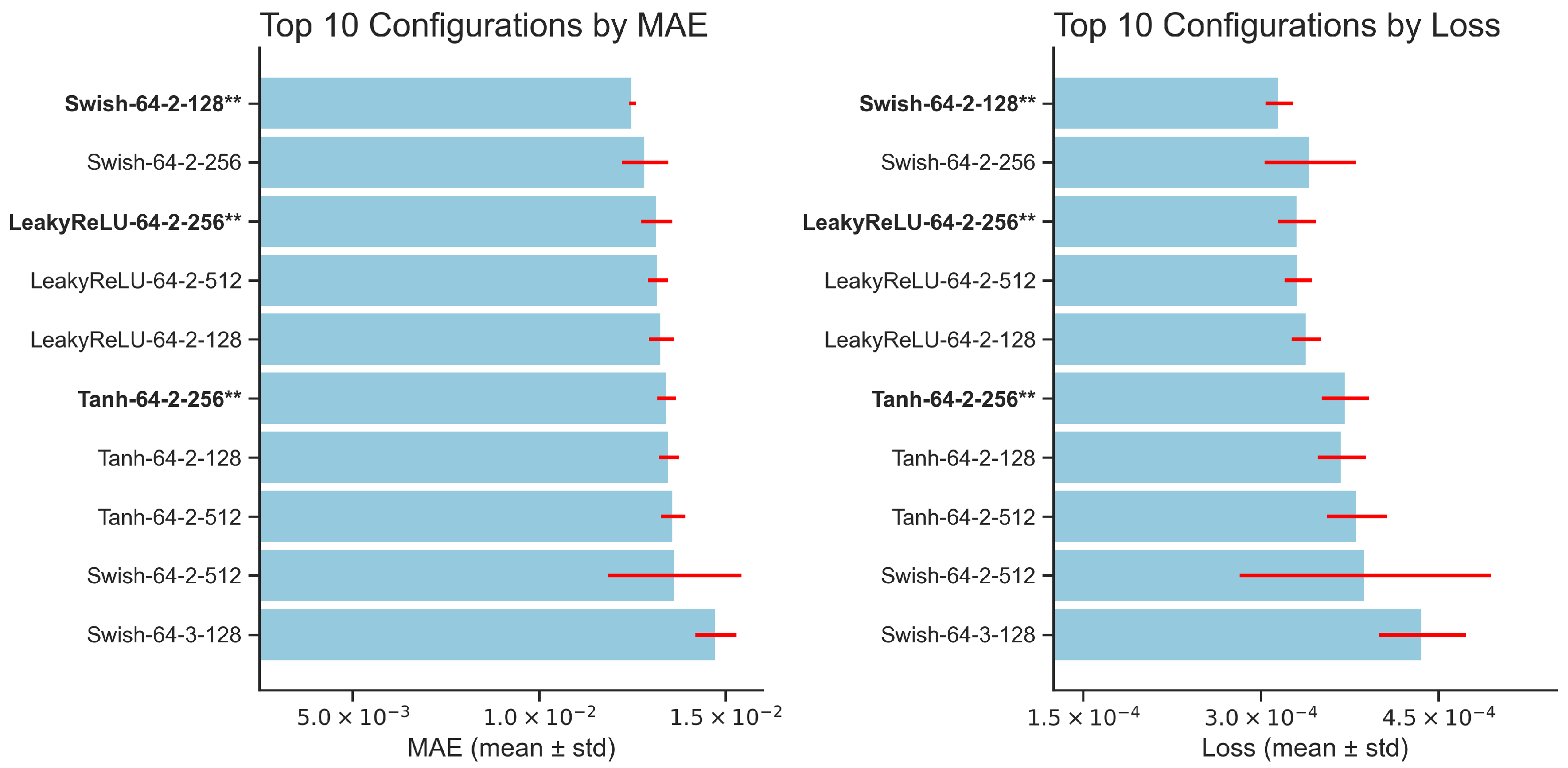
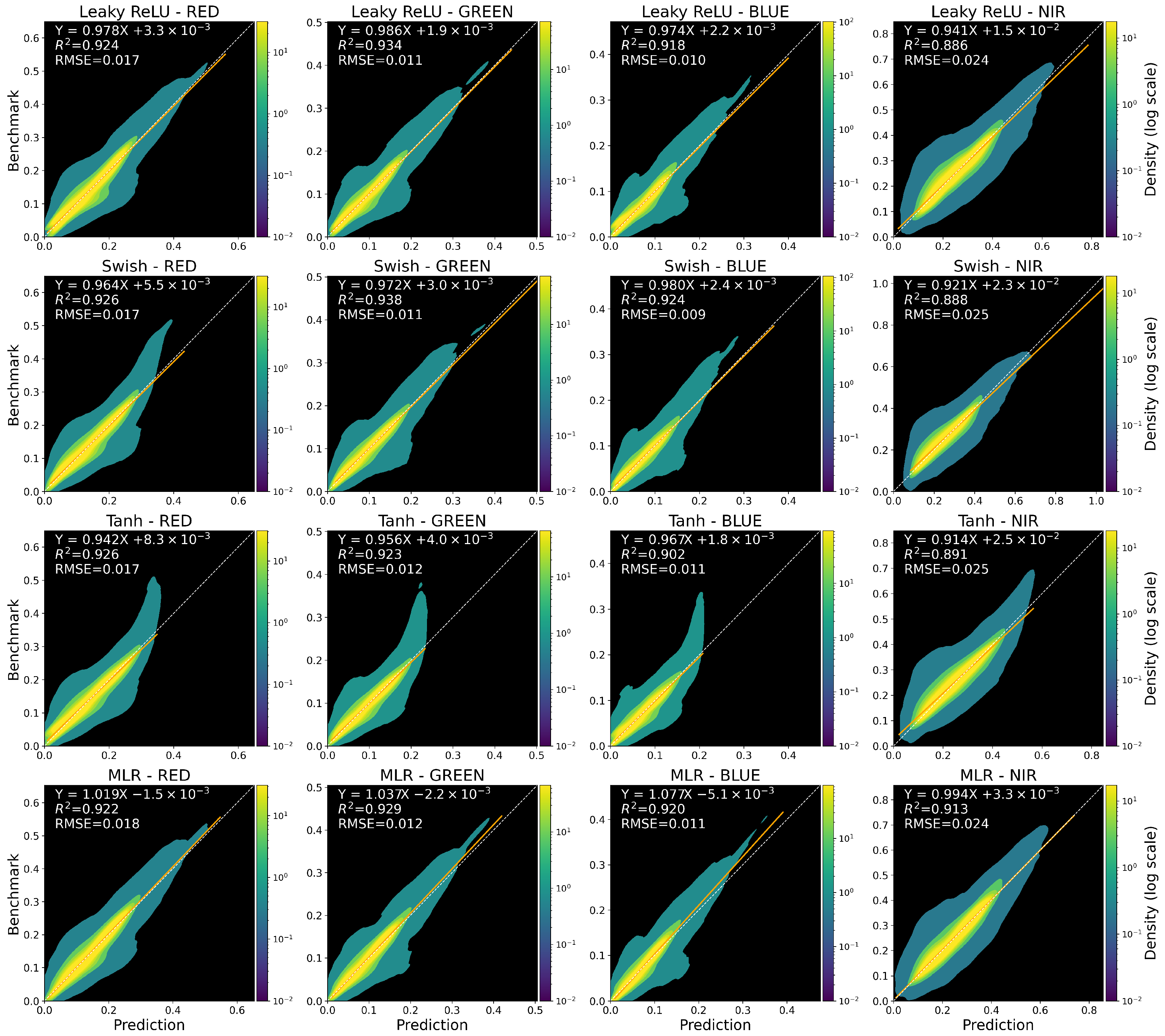
3.2.2. Feedforward Neural Network Regression Approach
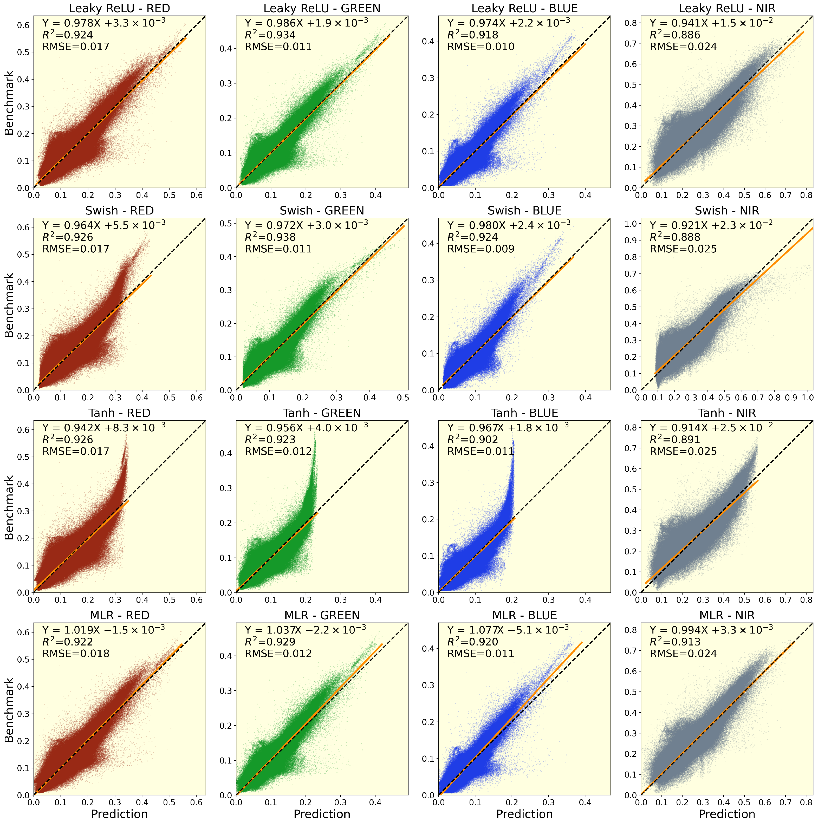
3.2.3. Global Evaluation of Machine Learning Models Performance
4. Discussion
4.1. Dataset Quality and Its Impact on Results
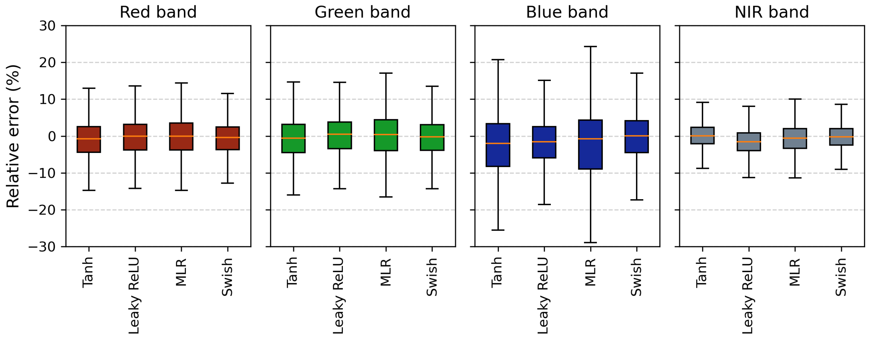
4.2. Machine Learning Model Performances by Spectral Band
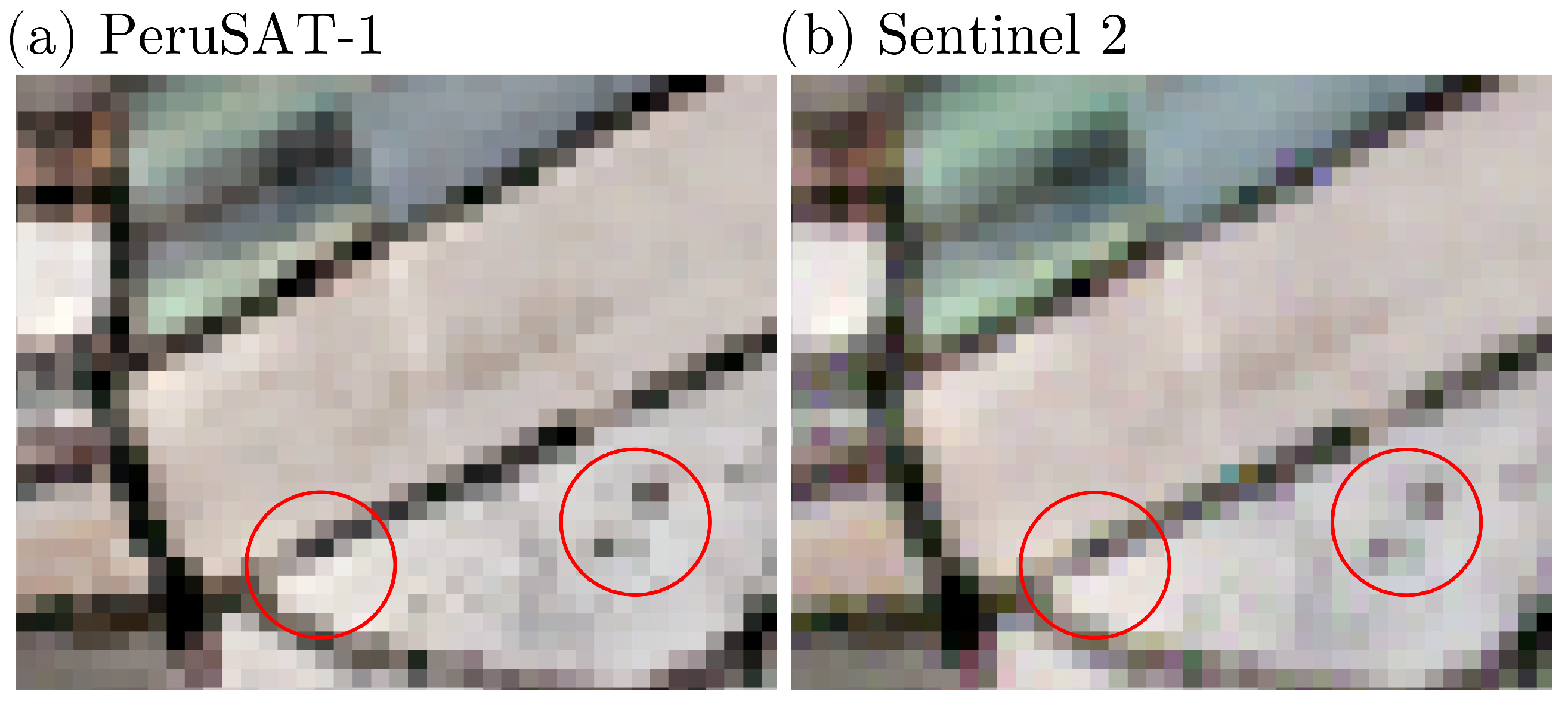
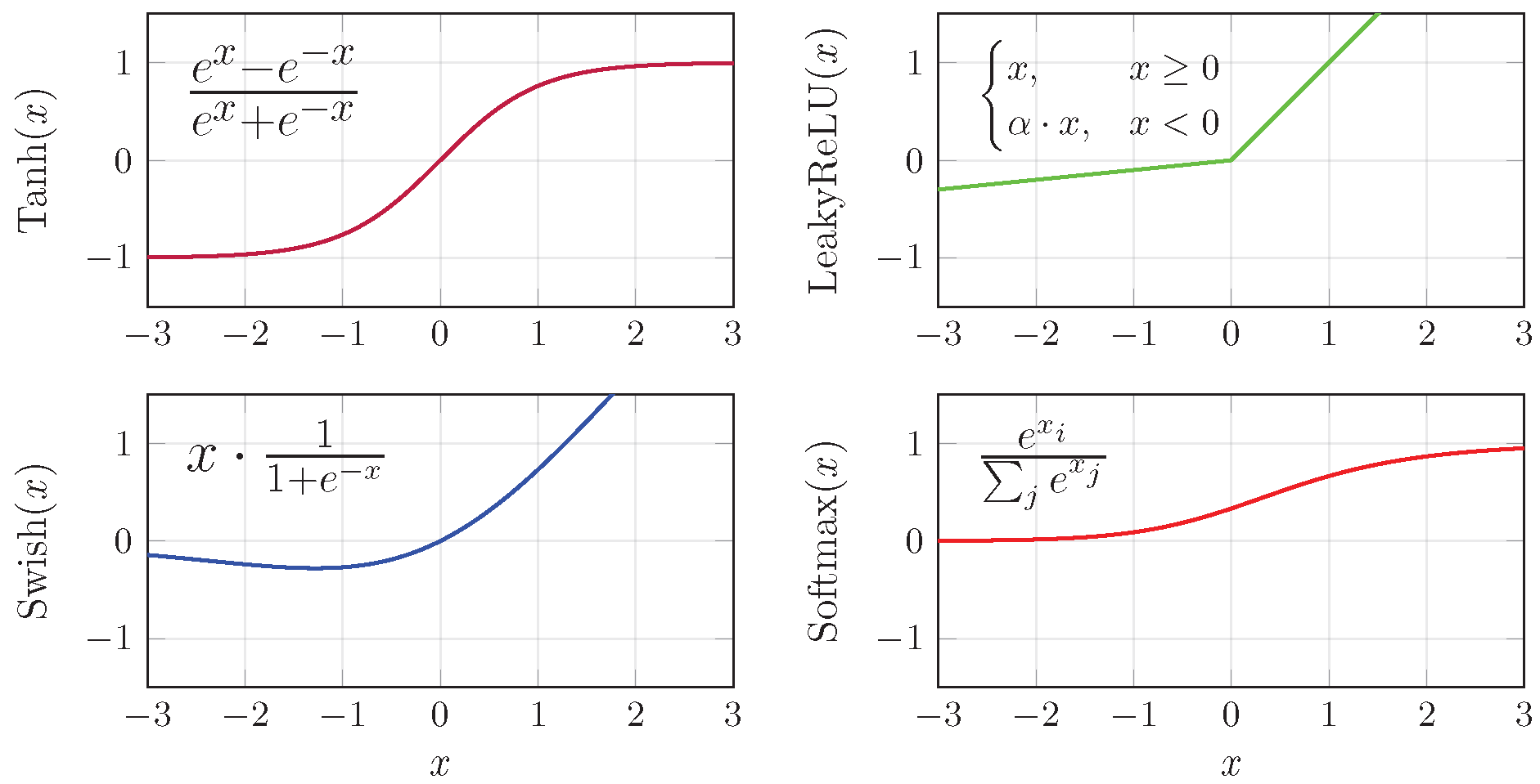
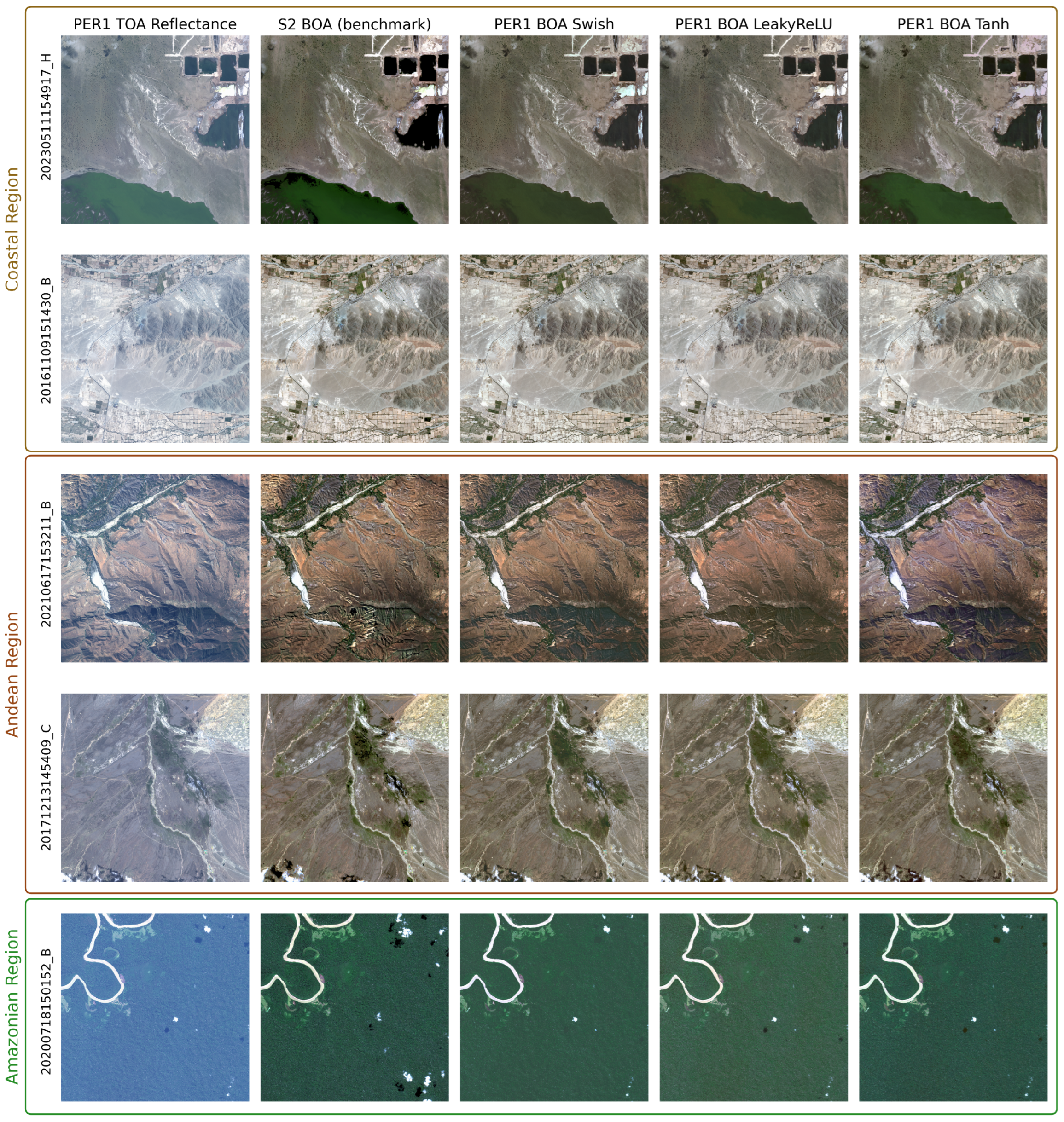
4.3. Effect of Activation Functions on Color
4.4. Seasonal Effect on Model Precision
4.5. Final Considerations and Future Directions
5. Conclusions
Author Contributions
Funding
Data Availability Statement
Acknowledgments
Conflicts of Interest
Abbreviations
| AOD | Aerosol Optical Depth |
| BOA | Bottom-of-Atmosphere |
| BRDF | Bidirectional Reflectance Distribution Function |
| CCL | Climate Classification Land |
| CNN | Convolutional Neural Network |
| CONIDA | Peruvian Space Agency (Agencia Espacial del Perú) |
| DEM | Digital Elevation Model |
| DS | Datastrip |
| FFNN | Feedforward Neural Network |
| GEE | Google Earth Engine |
| GSD | Ground Sample Distance |
| IGS | Image Ground Segment |
| L1C | Level-1C (Top-of-Atmosphere Sentinel-2 product) |
| L2A | Level-2A (Bottom-of-Atmosphere Sentinel-2 product) |
| L2H | Level-2H (Harmonized Sen2Like product) |
| LST | Local Solar Time |
| MAE | Mean Absolute Error |
| MLR | Multiple Linear Regression |
| MSE | Mean Squared Error |
| MS | Multispectral |
| MSI | Multispectral Instrument (Sentinel-2 sensor) |
| NAOMI | New AstroSat Optical Modular Instrument (PeruSAT-1 sensor) |
| NBAR | Nadir Bidirectional Reflectance Distribution Function-Adjusted Reflectance |
| NIR | Near-Infrared |
| OZ3 | Ozone |
| PAN | Panchromatic |
| PER1 | PeruSAT-1 |
| PC | Pearson Correlation |
| PMS | Pansharpened |
| R2 | Coefficient of Determination |
| RTM | Radiative Transfer Model |
| S2 | Sentinel-2 |
| SCL | Scene Classification Map |
| TOA | Top-of-Atmosphere |
| UTM | Universal Transverse Mercator |
| VHR | Very High Resolution |
| VIS | Visible |
| WGS84 | World Geodetic System 1984 |
| WVC | Water Vapor Column |
Appendix A. Variables and Data Sources Used in the Study

| Variables | Data Provider | Product | Data Range | Gridded Data |
|---|---|---|---|---|
| Primary Variables | ||||
| Aerosol Optical Depth (AOD) | ECMWF 1 | CAMS 2: “Total Aerosol Optical Depth at 550 nm” | 9.6 –3.58255 | 0.4° × 0.4° |
| Water Vapor Column (WVC) | NASA | MODIS MCD19A2 | 0–30 (cm) | 1000 m pixel |
| Nadir Bidirectional Reflectance Distribution Function Adjusted Reflectance (NBAR) | NASA | MODIS MCD43A4: - Band 1 (620–670 nm) - Band 2 (841–876 nm) - Band 3 (459–479 nm) - Band 4 (545–565 nm) | 0–3.2766 | 500 m pixel |
| Ozone (OZ3) | NASA | TOMS/MERGED | 73–983 (Dobson) | 1.0° × 1.0° |
| DEM | NASA | SRTM 90 | - | 90 m pixel |
| Climate Classification (CCL) | SENAMHI 3 | Peruvian Climate maps | 1–23 (classes) | - |
| Scene Classification Land (SCL) | ESA 4 | Sentinel-2–L2A SCL | 0–11 (classes) | 20 m pixel |
| TOA reflectance reference | ESA | S2–L1C | 0–1 (dimless) | 10 m pixel |
| BOA reflectance benchmark | ESA | S2–L2H | 0–1 | 10 m pixel |
| PER1 Data | CONIDA 5 | PER1–MS L3 | 0–4096 (DN) | 2.8 m pixel |
| Secondary Variables | ||||
| Terrain—Aspect | From DEM | Aspect map | 0°–360° | 10 m pixel |
| Terrain—Slope | From DEM | Slope map | 0°–90° | 10 m pixel |
| Terrain—Hill Shadows | From DEM | Hill shadows map | 0°–90° | 10 m pixel |
| PER1 Acquisition Geometry | CONIDA | Sensor & Sun Azimuth | 0°–180° | - |
| Sensor & Sun Zenith | 0°–90° |
Appendix B
Appendix C
| Activation Function | Sample | R2 Red | R2 Green | R2 Blue | R2 NIR |
|---|---|---|---|---|---|
| Swish | 20161109151430_B | 0.9646 | 0.9583 | 0.9505 | 0.9819 |
| 20171213145409_C | 0.9778 | 0.9754 | 0.9718 | 0.9750 | |
| 20200718150152_B | 0.7572 | 0.7915 | 0.7400 | 0.9526 | |
| 20210617153211_B | 0.9372 | 0.9336 | 0.9432 | 0.8968 | |
| 20230511154917_H | 0.9311 | 0.9292 | 0.9053 | 0.9114 | |
| Leaky ReLU | 20161109151430_B | 0.9519 | 0.9440 | 0.9431 | 0.9809 |
| 20171213145409_C | 0.9747 | 0.9726 | 0.9546 | 0.9719 | |
| 20200718150152_B | 0.7600 | 0.8708 | 0.7956 | 0.9518 | |
| 20210617153211_B | 0.9357 | 0.9336 | 0.9406 | 0.8965 | |
| 20230511154917_H | 0.9283 | 0.9253 | 0.8976 | 0.8923 | |
| Tanh | 20161109151430_B | 0.9667 | 0.9588 | 0.9499 | 0.9843 |
| 20171213145409_C | 0.9789 | 0.9752 | 0.9731 | 0.9760 | |
| 20200718150152_B | 0.8722 | 0.9087 | 0.8278 | 0.9559 | |
| 20210617153211_B | 0.9401 | 0.9398 | 0.9085 | 0.8987 | |
| 20230511154917_H | 0.9321 | 0.9277 | 0.9058 | 0.9224 |
Appendix D. Algorithmic Frameworks
| Algorithm A1: Geometry extraction for image sample cropping. | |
| 1: Input: (image path), (crop size, default = 3600), GeoTransform (coordinate transformation function) | |
| 2: Output: Shapefiles (SHP) with crop geometry | |
| 3: | ▷ is image matrix; is metadata |
| 4: | ▷ Number of rows (height) |
| 5: | ▷ Number of columns (width) |
| 6: if is not provided then | |
| 7: | ▷ Default crop size |
| 8: end if | |
| 9: | ▷ First row with data |
| 10: function Find_Initial_Row() | |
| 11: for to do | |
| 12: for to 0 do | |
| 13: if then | |
| 14: return y | ▷ Return first non-empty row |
| 15: end if | |
| 16: end for | |
| 17: end for | |
| 18: return H | ▷ Return height if no data is found |
| 19: end function | |
| 20: | ▷ Initial column |
| 21: | ▷ Number of crops |
| 22: for to do | |
| 23: | |
| 24: | |
| 25: | |
| 26: | |
| 27: | |
| 28: | |
| 29: SaveShapeFile(, ) | |
| 30: | ▷ Add separation between crops |
| 31: | |
| 32: end for | |
| 33: return Shapefiles | |
| Algorithm A2: Fixed k-means clustering for consistent classification. | ||
| 1: Input: (PER1 images), k (number of clusters), (excluded classes) | ||
| 2: Output: (binary masks) | ||
| 3: | ▷ Select reference image | |
| 4: | ▷ Compute water index for reference | |
| 5: | ▷ Augment image with water index | |
| 6: | ▷ Normalize augmented image | |
| 7: | ▷ Reshape image data into 2D array | |
| 8: | ▷ Fit k-means to reference image | |
| 9: for each in do | ▷ Iterate over all images | |
| 10: | ▷ Compute water index | |
| 11: | ▷ Augment image with water index | |
| 12: | ▷ Normalize augmented image | |
| 13: | ▷ Reshape image data into 2D array | |
| 14: | ▷ Predict clusters | |
| 15: for to do | ▷ Iterate over all pixels | |
| 16: | ▷ Create binary mask | |
| 17: end for | ||
| 18: end for | ||
| 19: return | ▷ Return binary masks for all images | |
| Algorithm A3: Contextual iterative data cleaning. | |
| 1: Input: (dataset), PER1 (target), S2 (slave), (Pearson correlation (PC) thresholds list), (initial threshold), (threshold step), (target PC values) | |
| 2: Output: (cleaned dataset), (linear coefficients) | |
| 3: | ▷ Filter invalid rows (e.g., NaNs, zeros) |
| 4: for do | ▷ Iterate over PC thresholds |
| 5: | |
| 6: for do | |
| 7: | |
| 8: | |
| 9: | ▷ Mean and covariance for m |
| 10: | |
| 11: while and do | |
| 12: | ▷ Mahalanobis distance |
| 13: | |
| 14: | ▷ Calculate PC |
| 15: if then | |
| 16: | |
| 17: break | |
| 18: else | |
| 19: | |
| 20: | |
| 21: end if | |
| 22: end while | |
| 23: if then | |
| 24: | |
| 25: end if | |
| 26: end for | |
| 27: | |
| 28: end for | |
| 29: return , | ▷ Return cleaned dataset and coefficients |
References
- Vaughan, R.A.; Jones, H.G. Remote Sensing of Vegetation: Principles, Techniques and Applications, 1st ed.; Oxford University Press: Oxford, UK, 2010. [Google Scholar]
- Campbell, J.B.; Wynne, R.H. Introduction to Remote Sensing, 5th ed.; Guilford Press: New York, NY, USA, 2011. [Google Scholar]
- Kaufman, Y.J. Atmospheric effect on spatial resolution of surface imagery. Appl. Opt. 1984, 23, 4164–4172. [Google Scholar] [CrossRef] [PubMed]
- Rech, B.; Hess, J.H. Effects of Atmospheric Correction on NDVI Retrieved From Sentinel 2 Imagery over Different Land Classes. Braz. Symp. Remote Sens. 2023, 20, 968–971. [Google Scholar]
- Wang, D.; Xiang, X.; Ma, R.; Guo, Y.; Zhu, W.; Wu, Z. A Novel Atmospheric Correction for Turbid Water Remote Sensing. Remote Sens. 2023, 15, 2091. [Google Scholar] [CrossRef]
- Zhou, Q.; Wang, S.; Liu, N.; Townsend, P.A.; Jiang, C.; Peng, B.; Verhoef, W.; Guan, K. Towards operational atmospheric correction of airborne hyperspectral imaging spectroscopy: Algorithm evaluation, key parameter analysis, and machine learning emulators. ISPRS J. Photogramm. Remote Sens. 2023, 196, 386–401. [Google Scholar] [CrossRef]
- Berk, A.; Conforti, P.; Kennett, R.; Perkins, T.; Hawes, F.; Van Den Bosch, J. MODTRAN® 6: A major upgrade of the MODTRAN® radiative transfer code. In Proceedings of the 2014 6th Workshop on Hyperspectral Image and Signal Processing: Evolution in Remote Sensing (WHISPERS), Lausanne, Switzerland, 24–27 June 2014; IEEE: Piscataway, NJ, USA, 2014; pp. 1–4. [Google Scholar] [CrossRef]
- Vermote, E.; Tanre, D.; Deuze, J.; Herman, M.; Morcette, J.J. Second Simulation of the Satellite Signal in the Solar Spectrum, 6S: An overview. IEEE Trans. Geosci. Remote Sens. 1997, 35, 675–686. [Google Scholar] [CrossRef]
- Chavez, P.S. An improved dark-object subtraction technique for atmospheric scattering correction of multispectral data. Remote Sens. Environ. 1988, 24, 459–479. [Google Scholar] [CrossRef]
- Bernstein, L.S. Quick atmospheric correction code: Algorithm description and recent upgrades. Opt. Eng. 2012, 51, 111719. [Google Scholar] [CrossRef]
- Gao, B.C.; Montes, M.J.; Davis, C.O.; Goetz, A.F. Atmospheric correction algorithms for hyperspectral remote sensing data of land and ocean. Remote Sens. Environ. 2009, 113, S17–S24. [Google Scholar] [CrossRef]
- Boardman, J.W. Post-ATREM polishing of AVIRIS apparent reflectance data using EFFORT: A lesson in accuracy versus precision. In Proceedings of the Summaries of the Seventh JPL Airborne Earth Science Workshop, Pasadena, CA, USA, 12–16 January 1998; Jet Propulsion Laboratory: Pasadena, CA, USA, 1998; Volume 1, p. 53. [Google Scholar]
- Pereira-Sandoval, M.; Ruescas, A.; Urrego, P.; Ruiz-Verdú, A.; Delegido, J.; Tenjo, C.; Soria-Perpinyà, X.; Vicente, E.; Soria, J.; Moreno, J. Evaluation of Atmospheric Correction Algorithms over Spanish Inland Waters for Sentinel-2 Multi Spectral Imagery Data. Remote Sens. 2019, 11, 1469. [Google Scholar] [CrossRef]
- Plotnikov, D.; Kolbudaev, P.; Matveev, A.; Proshin, A.; Polyanskiy, I. Accuracy Assessment of Atmospheric Correction of KMSS-2 Meteor-M #2.2 Data over Northern Eurasia. Remote Sens. 2023, 15, 4395. [Google Scholar] [CrossRef]
- Doxani, G.; Vermote, E.; Roger, J.C.; Gascon, F.; Adriaensen, S.; Frantz, D.; Hagolle, O.; Hollstein, A.; Kirches, G.; Li, F.; et al. Atmospheric Correction Inter-Comparison Exercise. Remote Sens. 2018, 10, 352. [Google Scholar] [CrossRef] [PubMed]
- Doxani, G.; Vermote, E.F.; Roger, J.C.; Skakun, S.; Gascon, F.; Collison, A.; De Keukelaere, L.; Desjardins, C.; Frantz, D.; Hagolle, O.; et al. Atmospheric Correction Inter-comparison eXercise, ACIX-II Land: An assessment of atmospheric correction processors for Landsat 8 and Sentinel-2 over land. Remote Sens. Environ. 2023, 285, 113412. [Google Scholar] [CrossRef]
- Badhan, M.; Shamsaei, K.; Ebrahimian, H.; Bebis, G.; Lareau, N.P.; Rowell, E. Deep Learning Approach to Improve Spatial Resolution of GOES-17 Wildfire Boundaries Using VIIRS Satellite Data. Remote Sens. 2024, 16, 715. [Google Scholar] [CrossRef]
- Yuan, S.; Zhu, S.; Luo, X.; Mu, B. A deep learning-based bias correction model for Arctic sea ice concentration towards MITgcm. Ocean. Model. 2024, 188, 102326. [Google Scholar] [CrossRef]
- Zhang, W.; Sun, Y.; Wu, Y.; Dong, J.; Song, X.; Gao, Z.; Pang, R.; Guoan, B. A deep-learning real-time bias correction method for significant wave height forecasts in the Western North Pacific. Ocean Model. 2024, 187, 102289. [Google Scholar] [CrossRef]
- Shah, M.; Raval, M. A Deep Learning Model for Atmospheric Correction of Satellite Images. Authorea Prepr. 2022. [Google Scholar] [CrossRef]
- Shah, M.; Raval, M.S.; Divakaran, S. A Deep Learning Perspective to Atmospheric Correction of Satellite Images. In Proceedings of the IGARSS 2022—2022 IEEE International Geoscience and Remote Sensing Symposium, Kuala Lumpur, Malaysia, 17–22 July 2022; IEEE: Piscataway, NJ, USA, 2022; pp. 346–349. [Google Scholar] [CrossRef]
- Basener, A.A.; Basener, B.B. Deep Learning of Radiative Atmospheric Transfer with an Autoencoder. In Proceedings of the 2022 12th Workshop on Hyperspectral Imaging and Signal Processing: Evolution in Remote Sensing (WHISPERS), Rome, Italy, 13–16 September 2022; IEEE: Piscataway, NJ, USA, 2022; pp. 1–7. [Google Scholar] [CrossRef]
- Men, J.; Tian, L.; Zhao, D.; Wei, J.; Feng, L. Development of a Deep Learning-Based Atmospheric Correction Algorithm for Oligotrophic Oceans. IEEE Trans. Geosci. Remote Sens. 2022, 60, 4210819. [Google Scholar] [CrossRef]
- Zhao, X.; Ma, Y.; Xiao, Y.; Liu, J.; Ding, J.; Ye, X.; Liu, R. Atmospheric correction algorithm based on deep learning with spatial-spectral feature constraints for broadband optical satellites: Examples from the HY-1C Coastal Zone Imager. ISPRS J. Photogramm. Remote Sens. 2023, 205, 147–162. [Google Scholar] [CrossRef]
- Hosain, M.T.; Jim, J.R.; Mridha, M.; Kabir, M.M. Explainable AI approaches in deep learning: Advancements, applications and challenges. Comput. Electr. Eng. 2024, 117, 109246. [Google Scholar] [CrossRef]
- Haider, S.N.; Zhao, Q.; Meran, B.K. Automated data cleaning for data centers: A case study. In Proceedings of the 2020 39th Chinese Control Conference (CCC), Shenyang, China, 27–29 July 2020; IEEE: Piscataway, NJ, USA, 2020; pp. 3227–3232. [Google Scholar] [CrossRef]
- Shah, M.; Raval, M.; Divakaran, S.; Patel, P. Study and Impact Analysis of Data Shift in Deep Learning Based Atmospheric Correction. In Proceedings of the IGARSS 2023—2023 IEEE International Geoscience and Remote Sensing Symposium, Pasadena, CA, USA, 16–21 July 2023; IEEE: Piscataway, NJ, USA, 2023; pp. 6728–6731. [Google Scholar] [CrossRef]
- SENAMHI. Climas del Perú: Resumen Ejecutivo [Climates of Peru: Executive Summary]; Government Report; Servicio Nacional de Meteorología e Hidrología del Perú (SENAMHI): Lima, Peru, 2023.
- McCoy, R.M. Field Methods in Remote Sensing; Guilford Press: New York, NY, USA, 2005. [Google Scholar]
- eoPortal Directory. PeruSAT-1 Earth Observation Minisatellite. Satellite Missions Catalogue. 2016. Available online: https://www.eoportal.org/satellite-missions/perusat-1#naomi-new-astrosat-optical-modular-instrument (accessed on 22 August 2024).
- Main-Knorn, M.; Pflug, B.; Louis, J.; Debaecker, V.; Müller-Wilm, U.; Gascon, F. Sen2Cor for Sentinel-2. In Image and Signal Processing for Remote Sensing XXIII, Proceedings of the SPIE Remote Sensing, Warsaw, Poland, 1–14 September 2017; Bruzzone, L., Bovolo, F., Benediktsson, J.A., Eds.; SPIE: Bellingham, WA, USA, 2017; p. 3. [Google Scholar] [CrossRef]
- Pignatale, F. Sen2Cor 2.11.00 Configuration and User Manual; ACRI-ST: Sophia-Antipolis, France, 2022; OMPC.TPZG.SUM.001. [Google Scholar]
- Louis, J.; Devignot, O.; Pessiot, L. Sen2like L2HF Product Definition Document 2022-1.1; Technical Report; European Space Agency (ESA): Paris, France, 2022. [Google Scholar]
- Clerc, S. MPC Team ARGANS. Level 2A Data Quality Report; Technical Report; European Space Agency (ESA): Paris, France, 2022; Issue 2.0, S2-PDGS-MPC-S2L-ATBD. [Google Scholar]
- European Space Agency (ESA). Sentinel-2 Harmonized Level-1C (L1C) Dataset. 2024. Available online: https://developers.google.com/earth-engine/datasets/catalog/COPERNICUS_S2_HARMONIZED#description (accessed on 19 January 2024).
- European Space Agency (ESA). Sentinel-2 Harmonized Level-2A (L2A) Dataset. 2024. Available online: https://developers.google.com/earth-engine/datasets/catalog/COPERNICUS_S2_SR_HARMONIZED#description (accessed on 19 January 2024).
- Louis, J.; Devignot, O.; Pessiot, L. Sen2like Algorithm Theoretical Basis Document 2022-2.0; Technical Report; European Space Agency (ESA): Paris, France, 2022; Issue 2.0, S2-PDGS-MPC-S2L-ATBD. [Google Scholar]
- Sabater, M.M. Development of Atmospheric Correction Algorithms for Very High Spectral and Spatial Resolution Images: Application to SEOSAT and the FLEX/Sentinel-3 Missions. Ph.D. Thesis, Universitat de València, Valencia, Spain, 2018. [Google Scholar]
- Lacherade, S.; Fougnie, B.; Henry, P.; Gamet, P. Cross Calibration Over Desert Sites: Description, Methodology, and Operational Implementation. IEEE Trans. Geosci. Remote Sens. 2013, 51, 1098–1113. [Google Scholar] [CrossRef]
- Mather, P.; Tso, B. Classification Methods for Remotely Sensed Data, 2nd ed.; CRC Press: Boca Raton, FL, USA, 2009. [Google Scholar] [CrossRef]
- Tong, X.; Ye, Z.; Xu, Y.; Gao, S.; Xie, H.; Du, Q.; Liu, S.; Xu, X.; Liu, S.; Luan, K.; et al. Image Registration with Fourier-Based Image Correlation: A Comprehensive Review of Developments and Applications. IEEE J. Sel. Top. Appl. Earth Obs. Remote Sens. 2019, 12, 4062–4081. [Google Scholar] [CrossRef]
- Alipour-Langouri, M.; Zheng, Z.; Chiang, F.; Golab, L.; Szlichta, J. Contextual Data Cleaning. In Proceedings of the 2018 IEEE 34th International Conference on Data Engineering Workshops (ICDEW), Paris, France, 16–20 April 2018; IEEE: Piscataway, NJ, USA, 2018; pp. 21–24. [Google Scholar] [CrossRef]
- Cabana, E.; Lillo, R.E.; Laniado, H. Multivariate outlier detection based on a robust Mahalanobis distance with shrinkage estimators. Stat. Pap. 2021, 62, 1583–1609. [Google Scholar] [CrossRef]
- Ramachandran, P.; Zoph, B.; Le, Q.V. Searching for Activation Functions. arXiv 2017, arXiv:1710.05941. [Google Scholar]
- Glorot, X.; Bengio, Y. Understanding the difficulty of training deep feedforward neural networks. In Proceedings of the Thirteenth International Conference on Artificial Intelligence and Statistics, Sardinia, Italy, 13–15 May 2010; Volume 9, pp. 249–256. [Google Scholar]
- Nwankpa, C.; Ijomah, W.; Gachagan, A.; Marshall, S. Activation Functions: Comparison of trends in Practice and Research for Deep Learning. arXiv 2018, arXiv:1811.03378. [Google Scholar] [CrossRef]
- Srivastava, N.; Hinton, G.; Krizhevsky, A.; Sutskever, I.; Salakhutdinov, R. Dropout: A Simple Way to Prevent Neural Networks from Overfitting. J. Mach. Learn. Res. 2014, 15, 1929–1958. [Google Scholar]
- Montavon, G.; Orr, G.B.; Müller, K.R. (Eds.) Neural Networks: Tricks of the Trade, 2nd ed.; Lecture Notes in Computer Science; Springer: Berlin/Heidelberg, Germany, 2012; Volume 7700. [Google Scholar] [CrossRef]
- Ioffe, S.; Szegedy, C. Batch Normalization: Accelerating Deep Network Training by Reducing Internal Covariate Shift. arXiv 2015, arXiv:1502.03167. [Google Scholar]
- Emmert-Streib, F.; Yang, Z.; Feng, H.; Tripathi, S.; Dehmer, M. An Introductory Review of Deep Learning for Prediction Models with Big Data. Front. Artif. Intell. 2020, 3, 4. [Google Scholar] [CrossRef]
- Emmert-Streib, F.; Dehmer, M. (Eds.) Deep Learning Models; MDPI: Basel, Switzerland, 2020. [Google Scholar]
- Bengio, Y. Learning Deep Architectures for AI. Found. Trends Mach. Learn. 2009, 2, 1–127. [Google Scholar] [CrossRef]
| Hyperparameter | Range |
|---|---|
| Initial neurons | 32–64 |
| Hidden layers | 2–3 |
| Batch size | 128–512 |
| Learning rate | 1 to 1 |
| L2 regularization weight | 1 to 1 |
| Dropout rate | 0.35–0.4 |
Disclaimer/Publisher’s Note: The statements, opinions and data contained in all publications are solely those of the individual author(s) and contributor(s) and not of MDPI and/or the editor(s). MDPI and/or the editor(s) disclaim responsibility for any injury to people or property resulting from any ideas, methods, instructions or products referred to in the content. |
© 2025 by the authors. Licensee MDPI, Basel, Switzerland. This article is an open access article distributed under the terms and conditions of the Creative Commons Attribution (CC BY) license (https://creativecommons.org/licenses/by/4.0/).
Share and Cite
Saldarriaga, L.; Tan, Y.; Sabater, N.; Delegido, J. A Pixel-Based Machine Learning Atmospheric Correction for PeruSAT-1 Imagery. Remote Sens. 2025, 17, 460. https://doi.org/10.3390/rs17030460
Saldarriaga L, Tan Y, Sabater N, Delegido J. A Pixel-Based Machine Learning Atmospheric Correction for PeruSAT-1 Imagery. Remote Sensing. 2025; 17(3):460. https://doi.org/10.3390/rs17030460
Chicago/Turabian StyleSaldarriaga, Luis, Yumin Tan, Neus Sabater, and Jesus Delegido. 2025. "A Pixel-Based Machine Learning Atmospheric Correction for PeruSAT-1 Imagery" Remote Sensing 17, no. 3: 460. https://doi.org/10.3390/rs17030460
APA StyleSaldarriaga, L., Tan, Y., Sabater, N., & Delegido, J. (2025). A Pixel-Based Machine Learning Atmospheric Correction for PeruSAT-1 Imagery. Remote Sensing, 17(3), 460. https://doi.org/10.3390/rs17030460