

Application of UAV Photogrammetry and Multispectral Image Analysis for Identifying Land Use and Vegetation Cover Succession in Former Mining Areas


Abstract
1. Introduction
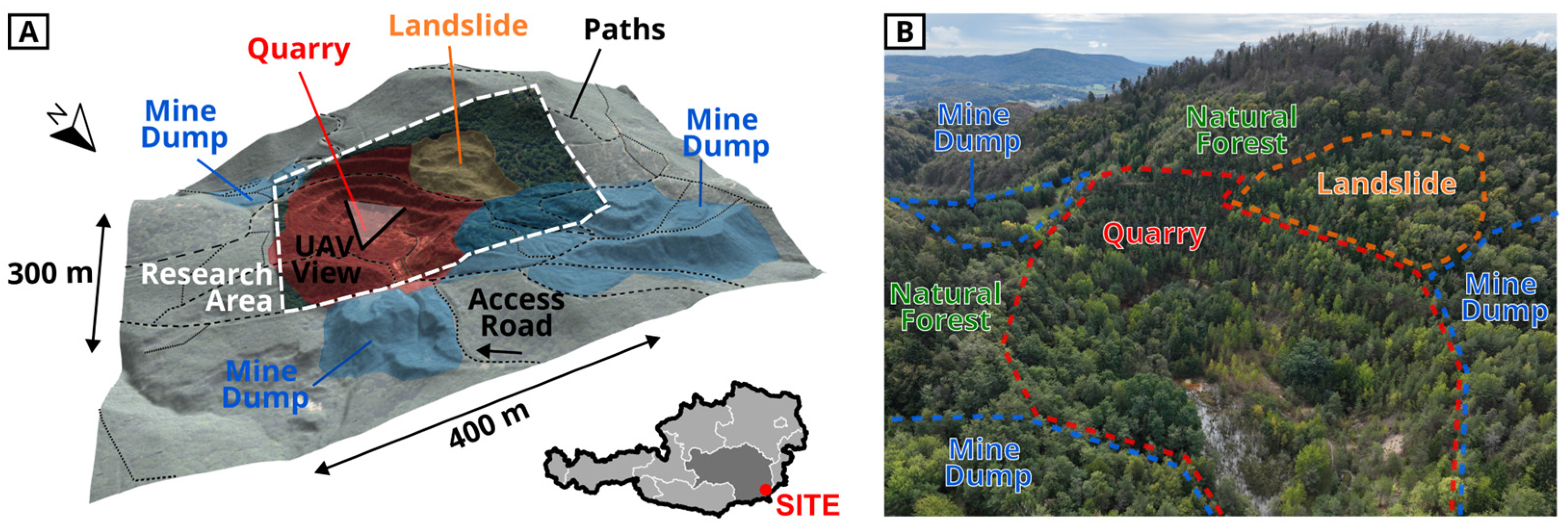
2. Study Site
3. Investigative Methods
3.1. UAV Mapping Flights
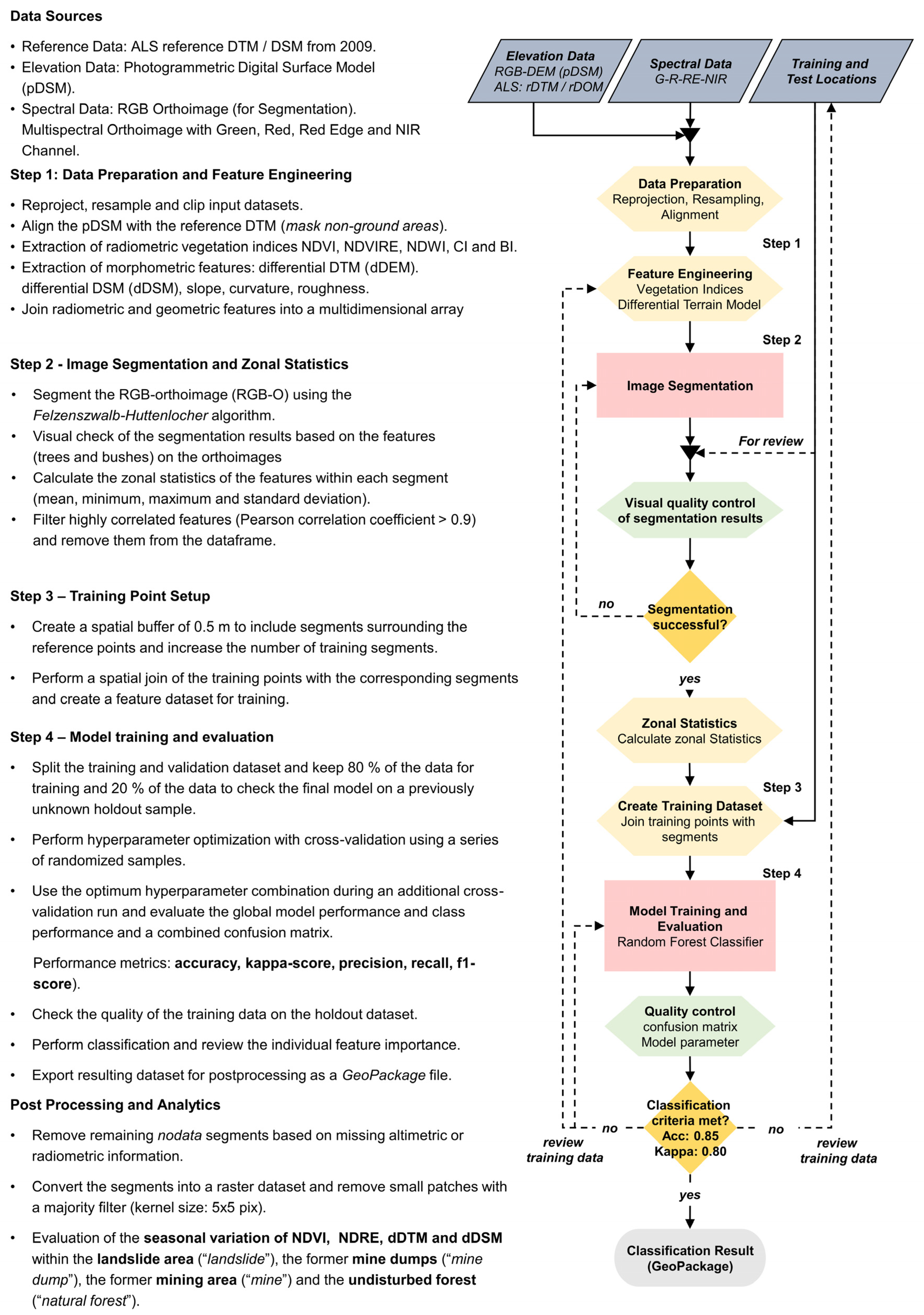
3.2. Object Based Image Classification and Analysis Workflow
3.2.1. Data Preparation and Feature Engineering (Step 1)
3.2.2. Image Segmentation and Zonal Statistics (Step 2)
3.2.3. Training Point Setup (Step 3)
3.2.4. Model Training and Evaluation (Step 4)
3.2.5. Post Processing and Analytics (Step 5)
4. Results
4.1. Photogrammetric Modeling and Image Segmentation Performance
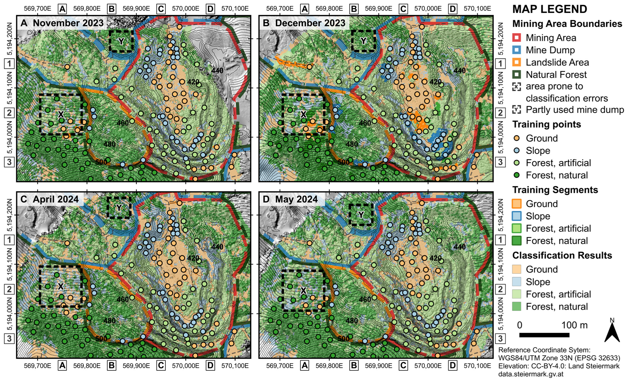
4.2. Classification Results
4.3. Temporal Variations in NDVI and Growth Height
5. Discussion
5.1. Flight Setup and Optimal Mapping Season
5.2. Application for Landcover Classification
5.3. Application for Vegetation Monitoring
6. Conclusions
- Small UAVs with combined multispectral and RGB camera systems provide a versatile and efficient platform for classifying and monitoring mining areas and forested landslides. Data acquisition and flight setup can be optimized for the specific site conditions to ensure representative and concise training data.
- The most effective period for data acquisition is at the end or beginning of the growing season during overcast conditions. The use of 8-bit imagery should be avoided as it interferes with the alignment process and the use of the irradiance sensor.
- High resolution geometric and radiometric data from UAVs provide optimal training features to obtain accurate classification models. The integration of a reference terrain model with repeated UAV flights enables differentiation between natural forest and former mining areas, as well as the determination of variable growth patterns.
- Disturbances in the forest cover resulting from earthworks and the regrowth of forest on former mining sites can be efficiently detected and classified. Morphological features (dDTM, dDSM, curvature, roughness) are the most relevant classification parameters, followed by the NDRE and the Brightness Index (BI).
- Vegetation patterns in the former mining areas and on the landslide have a different time-dependent variation compared to the surrounding natural forest. Variations in NDVI, NDRE, dDTM and dDSM exhibit characteristic temporal patterns, with their lowest values observed in December and their highest in May. Among these parameters, the NDRE demonstrated a relatively higher variance compared to the NDVI.
- Former mining areas are characterized by distinct spectral indices (both NDVI and NDRE) and demonstrate reduced variability in the growth height compared to natural forests (expressed by the dDTM and dDSM). This can be attributed to the presence of varying plant species (predominantly coniferous trees), the sparser vegetation and the younger age of the vegetation.
- Future applications of the methodology described herein could be used to optimize mine reclamation strategies, according to the monitoring results. This requires a reference dataset prior to reclamation activities and a series of repeated surveys during the reclamation. Additionally, the combined multispectral and geometrical data could provide an efficient supplement to DEM-based landslide monitoring concepts by differentiating between active and dormant landslide areas according to vegetation patterns.
Author Contributions
Funding
Data Availability Statement
Conflicts of Interest
References
- Avtar, R.; Watanabe, T. Unmanned Aerial Vehicle: Applications in Agriculture and Environment; Springer International Publishing: Cham, Switzerland, 2020; ISBN 978-3-030-27156-5. [Google Scholar]
- Rejeb, A.; Abdollahi, A.; Rejeb, K.; Treiblmaier, H. Drones in Agriculture: A Review and Bibliometric Analysis. Comput. Electron. Agric. 2022, 198, 107017. [Google Scholar] [CrossRef]
- Ecke, S.; Dempewolf, J.; Frey, J.; Schwaller, A.; Endres, E.; Klemmt, H.-J.; Tiede, D.; Seifert, T. UAV-Based Forest Health Monitoring: A Systematic Review. Remote Sens. 2022, 14, 3205. [Google Scholar] [CrossRef]
- Lusiana, N.; Shinohara, Y.; Imaizumi, F. Quantifying Effects of Changes in Forest Age Distribution on the Landslide Frequency in Japan. Nat. Hazards 2024, 120, 8551–8570. [Google Scholar] [CrossRef]
- Cabral, R.P.; Da Silva, G.F.; De Almeida, A.Q.; Bonilla-Bedoya, S.; Dias, H.M.; De Mendonça, A.R.; Rodrigues, N.M.M.; Valente, C.C.A.; Oliveira, K.; Gonçalves, F.G.; et al. Mapping of the Successional Stage of a Secondary Forest Using Point Clouds Derived from UAV Photogrammetry. Remote Sens. 2023, 15, 509. [Google Scholar] [CrossRef]
- Chen, C.; Li, C.; Huang, C.; Lin, H.; Zelený, D. Secondary Succession on Landslides in Submontane Forests of Central Taiwan: Environmental Drivers and Restoration Strategies. Appl. Veg. Sci. 2022, 25, e12635. [Google Scholar] [CrossRef]
- Choi, H.-W.; Kim, H.-J.; Kim, S.-K.; Na, W.S. An Overview of Drone Applications in the Construction Industry. Drones 2023, 7, 515. [Google Scholar] [CrossRef]
- Shahmoradi, J.; Talebi, E.; Roghanchi, P.; Hassanalian, M. A Comprehensive Review of Applications of Drone Technology in the Mining Industry. Drones 2020, 4, 34. [Google Scholar] [CrossRef]
- Sun, J.; Yuan, G.; Song, L.; Zhang, H. Unmanned Aerial Vehicles (UAVs) in Landslide Investigation and Monitoring: A Review. Drones 2024, 8, 30. [Google Scholar] [CrossRef]
- Ren, H.; Zhao, Y.; Xiao, W.; Hu, Z. A Review of UAV Monitoring in Mining Areas: Current Status and Future Perspectives. Int. J. Coal Sci. Technol. 2019, 6, 320–333. [Google Scholar] [CrossRef]
- Hu, J.; Ye, B.; Bai, Z.; Feng, Y. Remote Sensing Monitoring of Vegetation Reclamation in the Antaibao Open-Pit Mine. Remote Sens. 2022, 14, 5634. [Google Scholar] [CrossRef]
- Ilinca, V.; Șandric, I.; Chițu, Z.; Irimia, R.; Gheuca, I. UAV Applications to Assess Short-Term Dynamics of Slow-Moving Landslides under Dense Forest Cover. Landslides 2022, 19, 1717–1734. [Google Scholar] [CrossRef]
- Moudrý, V.; Gdulová, K.; Fogl, M.; Klápště, P.; Urban, R.; Komárek, J.; Moudrá, L.; Štroner, M.; Barták, V.; Solský, M. Comparison of Leaf-off and Leaf-on Combined UAV Imagery and Airborne LiDAR for Assessment of a Post-Mining Site Terrain and Vegetation Structure: Prospects for Monitoring Hazards and Restoration Success. Appl. Geogr. 2019, 104, 32–41. [Google Scholar] [CrossRef]
- Park, S.; Choi, Y. Applications of Unmanned Aerial Vehicles in Mining from Exploration to Reclamation: A Review. Minerals 2020, 10, 663. [Google Scholar] [CrossRef]
- Al Heib, M.M.; Franck, C.; Djizanne, H.; Degas, M. Post-Mining Multi-Hazard Assessment for Sustainable Development. Sustainability 2023, 15, 8139. [Google Scholar] [CrossRef]
- Guo, S.; Yang, S.; Liu, C. Mining Heritage Reuse Risks: A Systematic Review. Sustainability 2024, 16, 4048. [Google Scholar] [CrossRef]
- Meng, H.; Wu, J.; Zhang, C.; Wu, K. Mechanism Analysis and Process Inversion of the “7.26” Landslide in the West Open-Pit Mine of Fushun, China. Water 2023, 15, 2652. [Google Scholar] [CrossRef]
- Zapico, I.; Molina, A.; Laronne, J.B.; Sánchez Castillo, L.; Martín Duque, J.F. Stabilization by Geomorphic Reclamation of a Rotational Landslide in an Abandoned Mine next to the Alto Tajo Natural Park. Eng. Geol. 2020, 264, 105321. [Google Scholar] [CrossRef]
- Thapa, P.S.; Daimaru, H.; Yanai, S. Analyzing Vegetation Recovery and Erosion Status after a Large Landslide at Mt. Hakusan, Central Japan. Ecol. Eng. 2024, 198, 107144. [Google Scholar] [CrossRef]
- Fu, S.; De Jong, S.M.; Deijns, A.; Geertsema, M.; De Haas, T. The SWADE Model for Landslide Dating in Time Series of Optical Satellite Imagery. Landslides 2023, 20, 913–932. [Google Scholar] [CrossRef]
- Van Den Eeckhaut, M.; Kerle, N.; Hervás, J.; Supper, R. Mapping of Landslides Under Dense Vegetation Cover Using Object-Oriented Analysis and LiDAR Derivatives. In Landslide Science and Practice; Margottini, C., Canuti, P., Sassa, K., Eds.; Springer: Berlin/Heidelberg, Germany, 2013; pp. 103–109. ISBN 978-3-642-31324-0. [Google Scholar]
- Santangelo, M.; Cardinali, M.; Bucci, F.; Fiorucci, F.; Mondini, A.C. Exploring Event Landslide Mapping Using Sentinel-1 SAR Backscatter Products. Geomorphology 2022, 397, 108021. [Google Scholar] [CrossRef]
- Li, D.; Tang, X.; Tu, Z.; Fang, C.; Ju, Y. Automatic Detection of Forested Landslides: A Case Study in Jiuzhaigou County, China. Remote Sens. 2023, 15, 3850. [Google Scholar] [CrossRef]
- Reinprecht, V.; Klass, C.; Kieffer, S. Aerial Imagery for Geological Hazard Management in Alpine Catchments. Geomech. Tunn. 2024, 17, 553–560. [Google Scholar] [CrossRef]
- Lillesand, T.M.; Kiefer, R.W.; Chipman, J.W. Remote Sensing and Image Interpretation, 7th ed.; Wiley: Hoboken, NJ, USA, 2015; ISBN 978-1-118-34328-9. [Google Scholar]
- Fernández, T.; Pérez, J.; Cardenal, J.; Gómez, J.; Colomo, C.; Delgado, J. Analysis of Landslide Evolution Affecting Olive Groves Using UAV and Photogrammetric Techniques. Remote Sens. 2016, 8, 837. [Google Scholar] [CrossRef]
- Xu, Y.; Zhu, H.; Hu, C.; Liu, H.; Cheng, Y. Deep Learning of DEM Image Texture for Landform Classification in the Shandong Area, China. Front. Earth Sci. 2022, 16, 352–367. [Google Scholar] [CrossRef]
- Weber, L. Handbuch der Lagerstätten der Erze, Industrieminerale und Energierohstoffe Österreichs. In Archiv für Lagerstättenforschung; Geologische Bundesanst: Wien, Austria, 1997; ISBN 978-3-900312-98-5. [Google Scholar]
- Jauk, J. Der Gossendorfer Bergbau—Materialien Für Eine Bildungsbezogene Nachnutzung. Master‘s Thesis, Karl-Franzens Universität Graz, Graz, Austria, 2018. [Google Scholar]
- DJI Mavic 3M User Manual [v1.7] 2024.06. Available online: https://ag.dji.com/de/mavic-3-m/downloads (accessed on 2 January 2025).
- Qu, T.; Li, Y.; Zhao, Q.; Yin, Y.; Wang, Y.; Li, F.; Zhang, W. Drone-Based Multispectral Remote Sensing Inversion for Typical Crop Soil Moisture under Dry Farming Conditions. Agriculture 2024, 14, 484. [Google Scholar] [CrossRef]
- Deng, L.; Mao, Z.; Li, X.; Hu, Z.; Duan, F.; Yan, Y. UAV-Based Multispectral Remote Sensing for Precision Agriculture: A Comparison between Different Cameras. ISPRS J. Photogramm. Remote Sens. 2018, 146, 124–136. [Google Scholar] [CrossRef]
- BEV-APOS Austrian Positioning Service. Available online: www.bev.gv.at/Services/Produkte/Grundlagenvermessung/APOS (accessed on 2 January 2025).
- Liu, X.; Lian, X.; Yang, W.; Wang, F.; Han, Y.; Zhang, Y. Accuracy Assessment of a UAV Direct Georeferencing Method and Impact of the Configuration of Ground Control Points. Drones 2022, 6, 30. [Google Scholar] [CrossRef]
- James, M.R.; Robson, S. Mitigating Systematic Error in Topographic Models Derived from UAV and Ground-based Image Networks. Earth Surf. Process. Landf. 2014, 39, 1413–1420. [Google Scholar] [CrossRef]
- Jiménez-Jiménez, S.I.; Ojeda-Bustamante, W.; Marcial-Pablo, M.; Enciso, J. Digital Terrain Models Generated with Low-Cost UAV Photogrammetry: Methodology and Accuracy. IJGIISPRS Int. J. Geo-Inf. 2021, 10, 285. [Google Scholar] [CrossRef]
- Vautherin, J.; Rutishauser, S.; Schneider-Zapp, K.; Choi, H.F.; Chovancova, V.; Glass, A.; Strecha, C. Photogrammetric accuracy and modeling of rolling shutter cameras. ISPRS Ann. Photogramm. Remote Sens. Spat. Inf. Sci. 2016, III-3, 139–146. [Google Scholar] [CrossRef]
- AgiSoft LLC AgiSoft Metashape Professional (Version 1.8.1.). Available online: www.agisoft.com (accessed on 2 January 2025).
- Saczuk, E. Processing Multi-Spectral Imagery with Agisoft MetaShape Pro. 2020. Available online: https://pressbooks.bccampus.ca/ericsaczuk/ (accessed on 2 January 2025).
- Over, J.S.R.; Ritchie, A.C.; Brown, J.; Kranenburg, C.J. Processing Coastal Imagery with Agisoft Metashape Professional Edition, Version 1.6—Structure from Motion Workflow Documentation; USGS Open-File Report; USGS Publications Warehouse: Reston, VA, USA, 2021. [Google Scholar]
- Luhmann, T.; Robson, S.; Kyle, S.; Boehm, J. Close-Range Photogrammetry and 3D Imaging, 4th ed.; De Gruyter Stem: Boston, MA, USA, 2023; ISBN 978-3-11-102935-1. [Google Scholar]
- Blaschke, T. Object Based Image Analysis for Remote Sensing. ISPRS J. Photogramm. Remote Sens. 2010, 65, 2–16. [Google Scholar] [CrossRef]
- Castillejo-González, I.L.; López-Granados, F.; García-Ferrer, A.; Peña-Barragán, J.M.; Jurado-Expósito, M.; De La Orden, M.S.; González-Audicana, M. Object- and Pixel-Based Analysis for Mapping Crops and Their Agro-Environmental Associated Measures Using QuickBird Imagery. Comput. Electron. Agric. 2009, 68, 207–215. [Google Scholar] [CrossRef]
- Hossain, M.D.; Chen, D. Segmentation for Object-Based Image Analysis (OBIA): A Review of Algorithms and Challenges from Remote Sensing Perspective. ISPRS J. Photogramm. Remote Sens. 2019, 150, 115–134. [Google Scholar] [CrossRef]
- Clewley, D.; Bunting, P.; Shepherd, J.; Gillingham, S.; Flood, N.; Dymond, J.; Lucas, R.; Armston, J.; Moghaddam, M. A Python-Based Open Source System for Geographic Object-Based Image Analysis (GEOBIA) Utilizing Raster Attribute Tables. Remote Sens. 2014, 6, 6111–6135. [Google Scholar] [CrossRef]
- Hay, G.J.; Castilla, G. Object-based image analysis: Strengths, weaknesses, opportunities and threats (SWOT). In Proceedings of the 1st international Conference on Object-based Image Analysis (OBIA 2006), Salzburg, Austria, 4–5 July 2006; Available online: https://www.isprs.org/proceedings/XXXVI/4-C42/ (accessed on 2 January 2025).
- Amatya, P.; Kirschbaum, D.; Stanley, T.; Tanyas, H. Landslide Mapping Using Object-Based Image Analysis and Open Source Tools. Eng. Geol. 2021, 282, 106000. [Google Scholar] [CrossRef]
- Robson, B.A.; Bolch, T.; MacDonell, S.; Hölbling, D.; Rastner, P.; Schaffer, N. Automated Detection of Rock Glaciers Using Deep Learning and Object-Based Image Analysis. Remote Sens. Environ. 2020, 250, 112033. [Google Scholar] [CrossRef]
- Machala, M.; Zejdová, L. Forest Mapping Through Object-Based Image Analysis of Multispectral and LiDAR Aerial Data. Eur. J. Remote Sens. 2014, 47, 117–131. [Google Scholar] [CrossRef]
- Soille, P.J.; Ansoult, M.M. Automated Basin Delineation from Digital Elevation Models Using Mathematical Morphology. Signal Process. 1990, 20, 171–182. [Google Scholar] [CrossRef]
- Felzenszwalb, P.F.; Huttenlocher, D.P. Efficient Graph-Based Image Segmentation. Int. J. Comput. Vis. 2004, 59, 167–181. [Google Scholar] [CrossRef]
- Achanta, R.; Shaji, A.; Smith, K.; Lucchi, A.; Fua, P.; Süsstrunk, S. SLIC Superpixels Compared to State-of-the-Art Superpixel Methods. IEEE Trans. Pattern Anal. Mach. Intell. 2012, 34, 2274–2282. [Google Scholar] [CrossRef]
- Vedaldi, A.; Soatto, S. Quick Shift and Kernel Methods for Mode Seeking. In Computer Vision—ECCV 2008; Forsyth, D., Torr, P., Zisserman, A., Eds.; Lecture Notes in Computer Science; Springer: Berlin/Heidelberg, Germany, 2008; Volume 5305, pp. 705–718. ISBN 978-3-540-88692-1. [Google Scholar]
- Florinsky, I.V. Digital Terrain Analysis in Soil Science and Geology, 2nd ed.; Elsevier: London, UK, 2016; ISBN 978-0-12-804632-6. [Google Scholar]
- Horn, B.K.P. Hill Shading and the Reflectance Map. Proc. IEEE 1981, 69, 14–47. [Google Scholar] [CrossRef]
- Zevenbergen, L.W.; Thorne, C.R. Quantitative Analysis of Land Surface Topography. Earth Surf. Process. Landf. 1987, 12, 47–56. [Google Scholar] [CrossRef]
- Polykretis, C.; Grillakis, M.; Alexakis, D. Exploring the Impact of Various Spectral Indices on Land Cover Change Detection Using Change Vector Analysis: A Case Study of Crete Island, Greece. Remote Sens. 2020, 12, 319. [Google Scholar] [CrossRef]
- QGIS Development Team. QGIS Geographic Information System (Version 3.38.3). Available online: https://qgis.org (accessed on 2 January 2025).
- Gallatin, K.; Albon, C. Machine Learning with Python Cookbook: Practical Solutions from Preprocessing to Deep Learning, 2nd ed.; O’Reilly Media Inc.: Sebastopol, CA, USA, 2023; ISBN 978-1-09-813572-0. [Google Scholar]
- Harris, C.R.; Millman, K.J.; Van Der Walt, S.J.; Gommers, R.; Virtanen, P.; Cournapeau, D.; Wieser, E.; Taylor, J.; Berg, S.; Smith, N.J. Array Programming with NumPy. Nature 2020, 585, 357–362. [Google Scholar] [CrossRef]
- Pandas Development Team (Version 2.2.2). Available online: https://github.com/pandas-dev/pandas.git (accessed on 2 January 2025).
- Gillies, S. Rasterio: Geospatial Raster I/O for Programmers (Version 1.4.1). Available online: https://github.com/rasterio/rasterio.git (accessed on 2 January 2025).
- Jordahl, K.; Bossche, J.V.D.; Fleischmann, M.; Wasserman, J.; McBride, J.; Gerard, J.; Tratner, J.; Perry, M.; Badaracco, A.G.; Farmer, C. GeoPandas (Version 1.0.1). Available online: https://github.com/geopandas/geopandas.git (accessed on 2 January 2025).
- GeoUtils Contributors GeoUtils (Version 0.1.9). Available online: https://github.com/GlacioHack/geoutils.git (accessed on 2 January 2025).
- xDEM Contributors xDEM (Version 0.0.20). Available online: https://github.com/GlacioHack/xdem.git (accessed on 2 January 2025).
- OpenCV Contributors Open CV (Version 4.10.0). Available online: https://github.com/opencv/opencv.git (accessed on 2 January 2025).
- Van Der Walt, S.; Schönberger, J.L.; Nunez-Iglesias, J.; Boulogne, F.; Warner, J.D.; Yager, N.; Gouillart, E.; Yu, T. Scikit-Image: Image Processing in Python. PeerJ 2014, 2, e453. [Google Scholar] [CrossRef]
- Pedregosa, F.; Varoquaux, G.; Gramfort, A.; Michel, V.; Thirion, B.; Grisel, O.; Blondel, M.; Prettenhofer, P.; Weiss, R.; Dubourg, V.; et al. Scikit-Learn: Machine Learning in Python. J. Mach. Learn. Res. 2011, 12, 2826–2830. [Google Scholar]
- Nuth, C.; Kääb, A. Co-Registration and Bias Corrections of Satellite Elevation Data Sets for Quantifying Glacier Thickness Change. Cryosphere 2011, 5, 271–290. [Google Scholar] [CrossRef]
- Amr, T. Hands-on Machine Learning with Scikit-Learn and Scientific Python Toolkits: A Practical Guide to Implementing Supervised and Unsupervised Machine Learning Algorithms in Python; Packt: Birmingham, UK; Mumbai, India, 2020; ISBN 978-1-83882-604-8. [Google Scholar]
- Belgiu, M.; Drăguţ, L. Random Forest in Remote Sensing: A Review of Applications and Future Directions. ISPRS J. Photogramm. Remote Sens. 2016, 114, 24–31. [Google Scholar] [CrossRef]
- Gislason, P.O.; Benediktsson, J.A.; Sveinsson, J.R. Random Forests for Land Cover Classification. Pattern Recognit. Lett. 2006, 27, 294–300. [Google Scholar] [CrossRef]
- Rimal, Y.; Sharma, N.; Alsadoon, A. The Accuracy of Machine Learning Models Relies on Hyperparameter Tuning: Student Result Classification Using Random Forest, Randomized Search, Grid Search, Bayesian, Genetic, and Optuna Algorithms. Multimed. Tools Appl. 2024, 83, 74349–74364. [Google Scholar] [CrossRef]
- Landis, J.R.; Koch, G.G. The Measurement of Observer Agreement for Categorical Data. Biometrics 1977, 33, 159. [Google Scholar] [CrossRef]
- Burns, W.J.; Madin, I.P. Protocol for Inventory Mapping of Landslide Deposits from Light Detection and Ranging (Lidar) Imagery. Oregon Department of Geology and Mineral Industries Special Paper No. 42. 2009. Available online: https://pubs.oregon.gov/dogami/sp/p-SP-42.htm (accessed on 2 January 2025).
- Boiarskii, B. Comparison of NDVI and NDRE Indices to Detect Differences in Vegetation and Chlorophyll Content. J. Mech. Contin. Math. Sci. 2019, 4, 20–29. [Google Scholar] [CrossRef]
- Liu, M.; Zhan, Y.; Li, J.; Kang, Y.; Sun, X.; Gu, X.; Wei, X.; Wang, C.; Li, L.; Gao, H.; et al. Validation of Red-Edge Vegetation Indices in Vegetation Classification in Tropical Monsoon Region—A Case Study in Wenchang, Hainan, China. Remote Sens. 2024, 16, 1865. [Google Scholar] [CrossRef]
- McNicol, I.M.; Mitchard, E.T.A.; Aquino, C.; Burt, A.; Carstairs, H.; Dassi, C.; Modinga Dikongo, A.; Disney, M.I. To What Extent Can UAV Photogrammetry Replicate UAV LiDAR to Determine Forest Structure? A Test in Two Contrasting Tropical Forests. J. Geophys. Res. Biogeosci. 2021, 126, e2021JG006586. [Google Scholar] [CrossRef]
- European Commission. European Commission Regulation 2019/947 on the Rules and Procedures for the Operation of Unmanned Aircraft, 2019; Official Journal of the European Union; Publications Office of the European Union: Luxembourg, 2019; pp. 45–71. Available online: https://skybrary.aero/articles/regulation-2019947-rules-and-procedures-unmanned-aircraft (accessed on 2 January 2025).
- Maes, W.H.; Steppe, K. Perspectives for Remote Sensing with Unmanned Aerial Vehicles in Precision Agriculture. Trends Plant Sci. 2019, 24, 152–164. [Google Scholar] [CrossRef]
- Kameyama, S.; Sugiura, K. Effects of Differences in Structure from Motion Software on Image Processing of Unmanned Aerial Vehicle Photography and Estimation of Crown Area and Tree Height in Forests. Remote Sens. 2021, 13, 626. [Google Scholar] [CrossRef]
- Dislich, C.; Huth, A. Modelling the Impact of Shallow Landslides on Forest Structure in Tropical Montane Forests. Ecol. Model. 2012, 239, 40–53. [Google Scholar] [CrossRef]
- Buma, B.; Pawlik, Ł. Post-landslide Soil and Vegetation Recovery in a Dry, Montane System Is Slow and Patchy. Ecosphere 2021, 12, e03346. [Google Scholar] [CrossRef]
- Vachova, P.; Vach, M.; Skalicky, M.; Walmsley, A.; Berka, M.; Kraus, K.; Hnilickova, H.; Vinduskova, O.; Mudrak, O. Reclaimed Mine Sites: Forests and Plant Diversity. Diversity 2021, 14, 13. [Google Scholar] [CrossRef]
- Govi, D.; Pappalardo, S.E.; De Marchi, M.; Meggio, F. From Space to Field: Combining Satellite, UAV and Agronomic Data in an Open-Source Methodology for the Validation of NDVI Maps in Precision Viticulture. Remote Sens. 2024, 16, 735. [Google Scholar] [CrossRef]
- Dash, J.P.; Pearse, G.D.; Watt, M.S. UAV Multispectral Imagery Can Complement Satellite Data for Monitoring Forest Health. Remote Sens. 2018, 10, 1216. [Google Scholar] [CrossRef]
- Mutanga, O.; Skidmore, A.K. Narrow Band Vegetation Indices Overcome the Saturation Problem in Biomass Estimation. Int. J. Remote Sens. 2004, 25, 3999–4014. [Google Scholar] [CrossRef]
- Agrafiotis, P.; Georgopoulos, A. Comparative assessment of very high resolution satellite and aerial orthoimagers. Int. Arch. Photogramm. Remote Sens. Spat. Inf. Sci. 2015, XL-3/W2, 1–7. [Google Scholar] [CrossRef]


| Data Source | Symbol | Application and Extracted Features |
|---|---|---|
| RGB Orthoimage | RGB-O | Used for Image Segmentation |
| RGB Digital Surface Model | pDSM | Used for morphometric feature extraction: slope, curvature, roughness, dDEM, dDSM |
| Multispectral Orthoimage | MS-O | Used for spectral feature extraction: NDVI: Normalized differential vegetation index: (NIR − Red)/(NIR + Red) NDRE: Normalized differential Red Edge (RE) index: (NIR − RE)/(NIR + RE) NDWI: Normalized differential water index: (Green − NIR)/(Green + NIR) CI: Coloration Index: (Green − Red)/(Green + Red) BI: Brightness Index: (((Red × Red)/(Green × Green)) × 0.5)0.5 |
| ALS Digital Terrain Model Date: 2009; Resolution 1 × 1 m | rDTM | Used for vertical co-registration and the calculation of the height above the (dDEM) |
| ALS Digital Surface Model Date: 2009; Resolution 1 × 1 m | rDSM | Used to calculate height above surface model (dDSM) |
| Flight Epoch | Illumination Condition | Flight Setup/ Image Datatype | GSD RGB/MS [cm/pix] | RE RGB/MS [pix] |
|---|---|---|---|---|
| 18 November 2023 | Sunny | Oblique/16-Bit Tiff | 3.3/4.8 | 0.7/0.4 |
| 29 December 2023 | Overcast | Nadir/8-Bit Tiff | 3.0/5.1 | 0.6/1.0 |
| 6 April 2024 | Overcast | Nadir/16-Bit Tiff | 2.9/5.0 | 0.5/0.5 |
| 25 May 2024 | Sunny | Nadir/16-Bit Tiff | 2.9/4.4 | 0.4/0.5 |
| Method | Algorithm Runtime | Average Segment Size [pix/m2] | Number of Segments [Count] | Classification Accuracy |
|---|---|---|---|---|
| Felzenswalb | 1.0 × Felzenswalb | 9.5/0.95 | 75,776 | 0.93 |
| Quickshift | 5.3 × Felzenswalb | 5.9/0.59 | 145,252 | 0.89 |
| Watershed | 7.1 × Felzenswalb | 4.7/0.47 | 79,920 | 0.82 |
| SLIC | 0.4 × Felzenswalb | 2.5/0.25 | 68,383 | 0.86 |
Disclaimer/Publisher’s Note: The statements, opinions and data contained in all publications are solely those of the individual author(s) and contributor(s) and not of MDPI and/or the editor(s). MDPI and/or the editor(s) disclaim responsibility for any injury to people or property resulting from any ideas, methods, instructions or products referred to in the content. |
© 2025 by the authors. Licensee MDPI, Basel, Switzerland. This article is an open access article distributed under the terms and conditions of the Creative Commons Attribution (CC BY) license (https://creativecommons.org/licenses/by/4.0/).
Share and Cite
Reinprecht, V.; Kieffer, D.S. Application of UAV Photogrammetry and Multispectral Image Analysis for Identifying Land Use and Vegetation Cover Succession in Former Mining Areas. Remote Sens. 2025, 17, 405. https://doi.org/10.3390/rs17030405
Reinprecht V, Kieffer DS. Application of UAV Photogrammetry and Multispectral Image Analysis for Identifying Land Use and Vegetation Cover Succession in Former Mining Areas. Remote Sensing. 2025; 17(3):405. https://doi.org/10.3390/rs17030405
Chicago/Turabian StyleReinprecht, Volker, and Daniel Scott Kieffer. 2025. "Application of UAV Photogrammetry and Multispectral Image Analysis for Identifying Land Use and Vegetation Cover Succession in Former Mining Areas" Remote Sensing 17, no. 3: 405. https://doi.org/10.3390/rs17030405
APA StyleReinprecht, V., & Kieffer, D. S. (2025). Application of UAV Photogrammetry and Multispectral Image Analysis for Identifying Land Use and Vegetation Cover Succession in Former Mining Areas. Remote Sensing, 17(3), 405. https://doi.org/10.3390/rs17030405