
Re-Using Historical Aerial Imagery for Obtaining 3D Data of Beach-Dune Systems: A Novel Refinement Method for Producing Precise and Comparable DSMs

 ,
,  , and
, and 
Abstract
1. Introduction
2. Materials and Methods
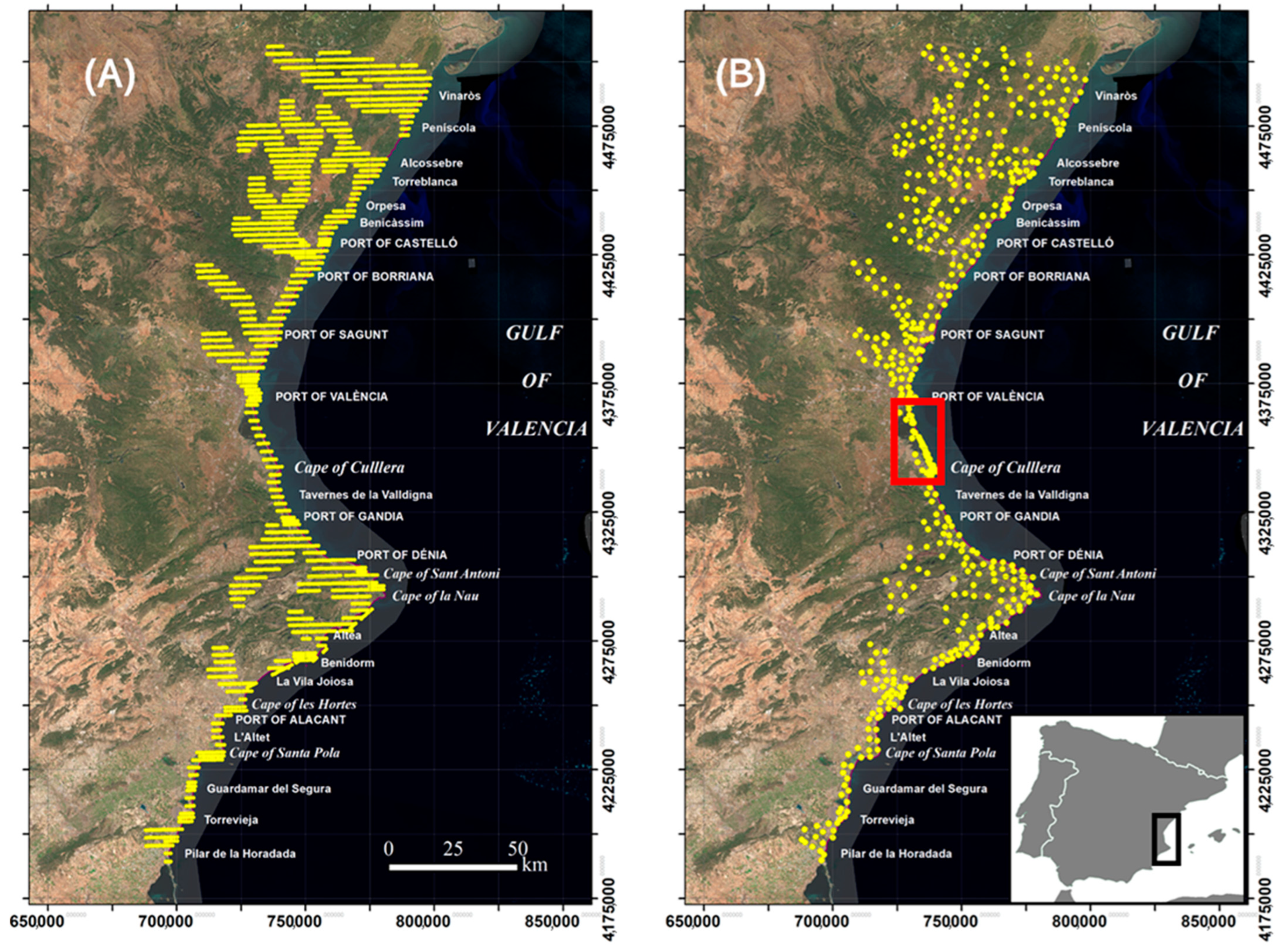
2.1. Materials and Study Site
2.2. Methodology
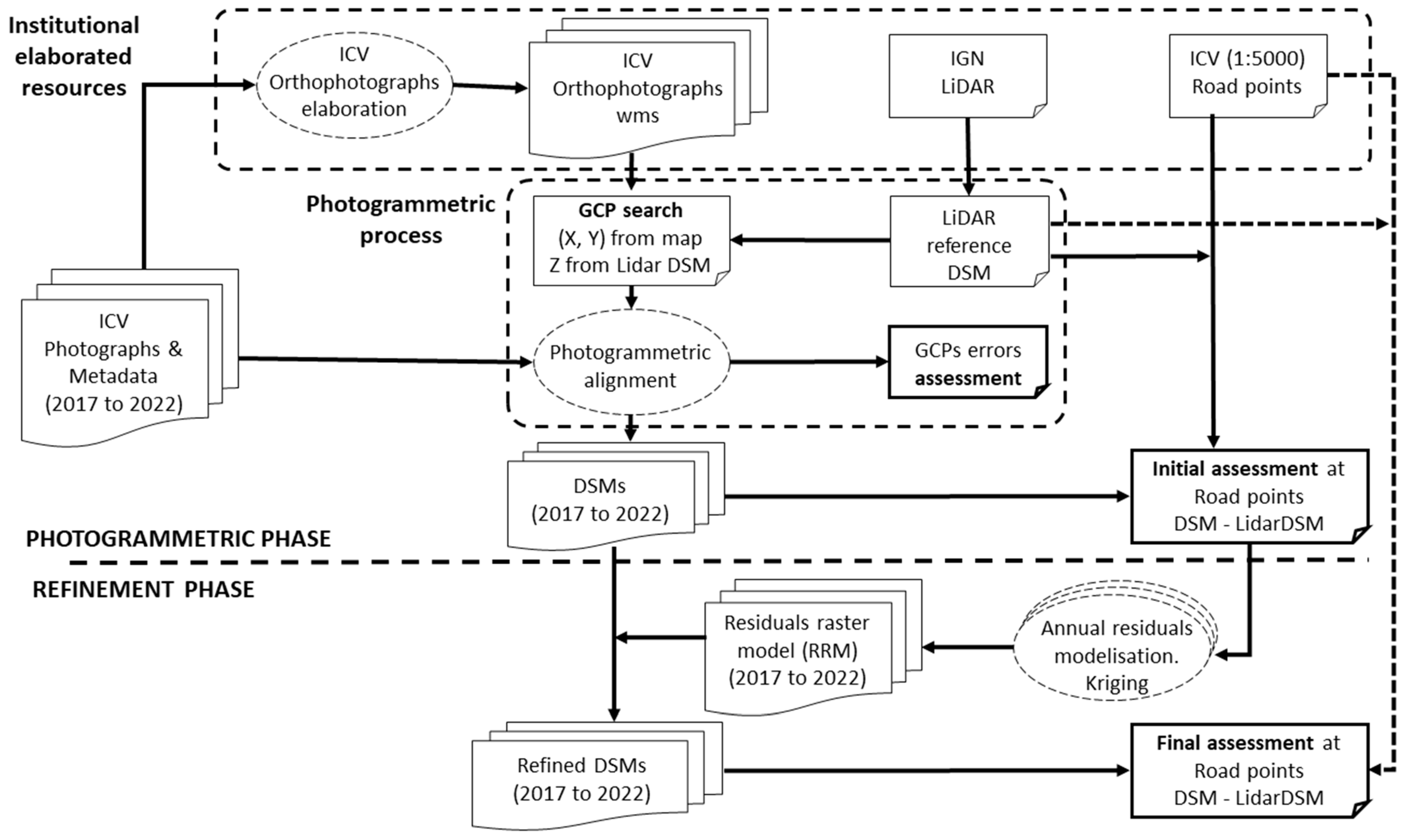
2.2.1. DSM: Photogrammetric and Refinement Processes
Photogrammetric Process
DSM Refinement
2.2.2. Volumetric Change Measurement: Example of Application for Quantifying Sediment Changes on the Valencian Coast
3. Results
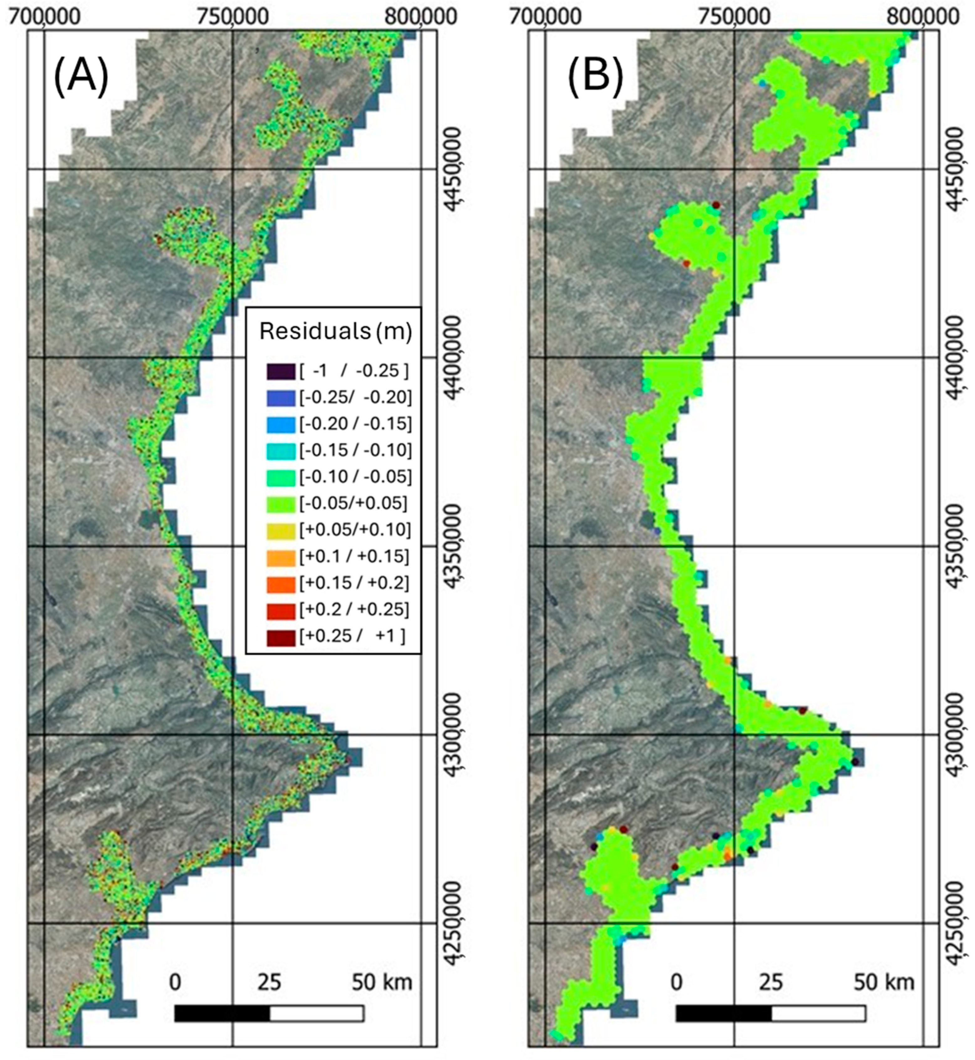
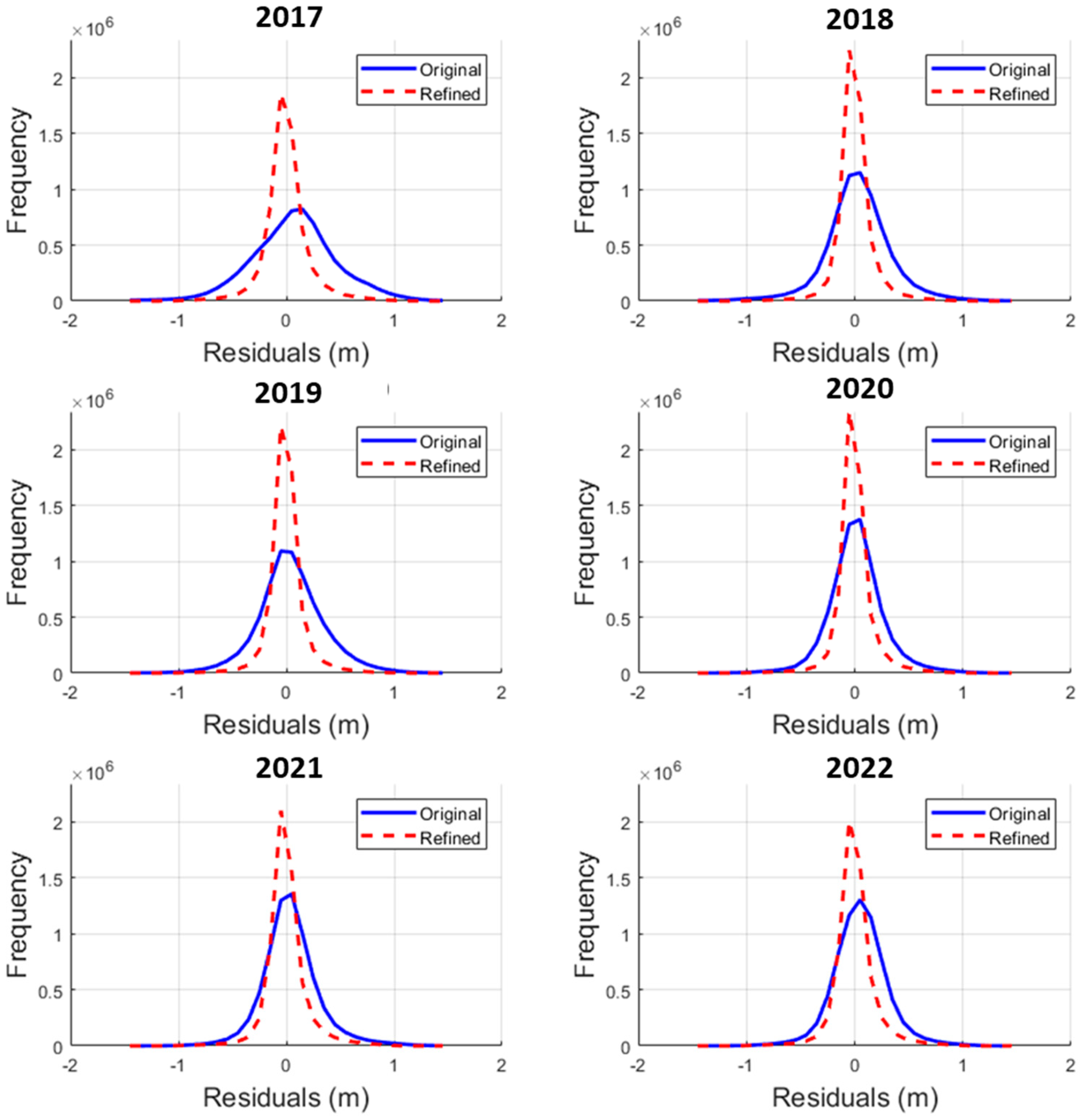
3.1. DSM: Photogrammetry and Refinement
3.2. Volume Change Assessment
4. Discussion
5. Conclusions
Author Contributions
Funding
Data Availability Statement
Acknowledgments
Conflicts of Interest
References
- Short, A.; Hesp, P. Wave, beach and dune interactions in southeastern Australia. Marine Geol. 1982, 48, 259–284. [Google Scholar] [CrossRef]
- Suanez, S.; Cariolet, J.; Cancouët, R.; Ardhuin, F.; Delacourt, C. Dune recovery after storm erosion on a high-energy beach: Vougot Beach, Brittany (France). Geomorphology 2011, 139–140, 16–33. [Google Scholar] [CrossRef]
- Zhang, K.; Douglas, B.C.; Leatherman, S.P. Global Warming and Coastal Erosion. Clim. Change 2004, 64, 41–58. [Google Scholar] [CrossRef]
- Pikelj, K.; Ružić, I.; Ilić, S.; James, M.R.; Kordić, B. Implementing an efficient beach erosion monitoring system for coastal management in Croatia. Ocean Coast. Manag. 2017, 156, 223–238. [Google Scholar] [CrossRef]
- Eamer, J.B.; Walker, I.J. Quantifying spatial and temporal trends in beach–dune volumetric changes using spatial statistics. Geomorphology 2013, 191, 94–108. [Google Scholar] [CrossRef]
- Turner, I.L.; Harley, M.D.; Short, A.D.; Simmons, J.A.; Bracs, M.A.; Phillips, M.S.; Splinter, K.D. A multi-decade dataset of monthly beach profile surveys and inshore wave forcing at Narrabeen, Australia. Sci. Data 2016, 3, 160024. [Google Scholar] [CrossRef] [PubMed]
- Pianca, C.; Holman, R.; Siegle, E. Shoreline variability from days to decades: Results of long-term video imaging. J. Geophys. Res. Ocean. 2015, 120, 2159–2178. [Google Scholar] [CrossRef]
- Ludka, B.C.; Guza, R.T.; O’Reilly, W.C.; Merrifield, M.A.; Flick, R.E.; Bak, A.S.; Hesser, T.; Bucciarelli, R.; Olfe, C.; Woodward, B.; et al. Sixteen years of bathymetry and waves at San Diego beaches. Sci. Data 2019, 6, 161. [Google Scholar] [CrossRef] [PubMed]
- Castelle, B.; Bujan, S.; Marieu, V.; Ferreira, S. 16 years of topographic surveys of rip-channelled high-energy meso-macrotidal sandy beach. Sci. Data 2020, 7, 410. [Google Scholar] [CrossRef] [PubMed]
- Melet, A.; Teatini, P.; Cozannet, G.L.; Jamet, C.; Conversi, A.; Benveniste, J.; Almar, R. Earth Observations for Monitoring Marine Coastal Hazards and Their Drivers. Surv. Geophys. 2020, 41, 1489–1534. [Google Scholar] [CrossRef]
- Chen, C.; Zhang, C.; Tian, B.; Wu, W.; Zhou, Y. Tide2Topo: A new method for mapping intertidal topography accurately in complex estuaries and bays with time-series Sentinel-2 images. ISPRS J. Photogramm. Remote Sens. 2023, 200, 55–72. [Google Scholar] [CrossRef]
- Chen, C.; Zhang, C.; Tian, B.; Wu, W.; Zhou, Y. Mapping intertidal topographic changes in a highly turbid estuary using dense Sentinel-2 time series with deep learning. ISPRS J. Photogramm. Remote Sens. 2023, 205, 1–16. [Google Scholar] [CrossRef]
- Zhang, X.; Zuo, L.; Lu, Y.; Li, H.; Zhao, Y. An improved approach for retrieval of tidal flat elevation based on inundation frequency. Estuar. Coast. Shelf Sci. 2025, 313, 109061. [Google Scholar] [CrossRef]
- Vos, K.; Splinter, K.D.; Palomar-Vázquez, J.; Pardo-Pascual, J.E.; Almonacid-Caballer, J.; Cabezas-Rabadán, C.; Kras, E.C.; Luijendijk, A.P.; Calkoen, F.; Almeida, L.P.; et al. Benchmarking satellite-derived shoreline mapping algorithms. Commun. Earth Environ. 2023, 4, 345. [Google Scholar] [CrossRef]
- Billet, C.; Alonso, G.; Danieli, G.; Dragani, W. Evaluation of beach nourishment in Mar del plata, Argentina: An application of the CoastSat toolkit. Coast. Eng. 2024, 193, 104593. [Google Scholar] [CrossRef]
- Cabezas-Rabadán, C.; Pardo-Pascual, J.; Palomar-Vázquez, J.; Roch-Talens, A.; Guillén, J. Satellite observations of storm erosion and recovery of the Ebro Delta coastline, NE Spain. Coast. Eng. 2024, 188, 104451. [Google Scholar] [CrossRef]
- De Urbaneja, I.C.B.; Pardo-Pascual, J.E.; Cabezas-Rabadán, C.; Aguirre, C.; Martínez, C.; Pérez-Martínez, W.; Palomar-Vázquez, J. Characterization of Multi-Decadal Beach Changes in Cartagena Bay (Valparaíso, Chile) from Satellite Imagery. Remote Sens. 2024, 16, 2360. [Google Scholar] [CrossRef]
- Castelle, B.; Ritz, A.; Marieu, V.; Lerma, A.N.; Vandenhove, M. Primary drivers of multidecadal spatial and temporal patterns of shoreline change derived from optical satellite imagery. Geomorphology 2022, 413, 108360. [Google Scholar] [CrossRef]
- Vos, K.; Harley, M.D.; Splinter, K.D.; Simmons, J.A.; Turner, I.L. Sub-annual to multi-decadal shoreline variability from publicly available satellite imagery. Coast. Eng. 2019, 150, 160–174. [Google Scholar] [CrossRef]
- Da Silva, P.G.; Jara, M.S.; Medina, R.; Beck, A.; Taji, M.A. On the use of satellite information to detect coastal change: Demonstration case on the coast of Spain. Coast. Eng. 2024, 191, 104517. [Google Scholar] [CrossRef]
- Hodgson, M.E.; Bresnahan, P. Accuracy of Airborne Lidar-Derived Elevation. Photogramm. Eng. Remote Sens. 2004, 70, 331–339. [Google Scholar] [CrossRef]
- Kakoulaki, G.; Martinez, A.; Florio, P. Non-Commercial Light Detection and Ranging (LiDAR) Data in Europe, EUR 30817 EN; Publications Office of the European Union: Luxembourg, 2021; ISBN 978-92-76-41150-5. JRC126223. [Google Scholar] [CrossRef]
- Mauff, B.L.; Juigner, M.; Ba, A.; Robin, M.; Launeau, P.; Fattal, P. Coastal monitoring solutions of the geomorphological response of beach-dune systems using multi-temporal LiDAR datasets (Vendée coast, France). Geomorphology 2018, 304, 121–140. [Google Scholar] [CrossRef]
- Saye, S.; Van Der Wal, D.; Pye, K.; Blott, S. Beach–dune morphological relationships and erosion/accretion: An investigation at five sites in England and Wales using LIDAR data. Geomorphology 2005, 72, 128–155. [Google Scholar] [CrossRef]
- Gosh, S.K. History of Photogrammetry—Analytical Methods and Instruments. In Proceedings of the ISPRS Archives—Volume XXIX Part B6, 1992, XVIIth ISPRS Congress Technical Commission VI: Economic, Professional and Eductional Apsects of Photogrammetry and Remote Sensing, Washington, DC, USA, 2–14 August 1992. [Google Scholar]
- Zhang, L.; Liu, Y.; Sun, Y.; Lan, C.; Al, H.; Fan, Z. A review of developments in the theory and technology of three-dimensional reconstruction in digital aerial photogrammetry. Acta Geod. Cartogr. Sin. 2022, 51, 1437–1457. [Google Scholar]
- Marín-Buzón, C.; Pérez-Romero, A.; López-Castro, J.L.; Jerbania, I.B.; Manzano-Agugliaro, F. Photogrammetry as a New Scientific Tool in Archaeology: Worldwide Research Trends. Sustainability 2021, 13, 5319. [Google Scholar] [CrossRef]
- Bakker, M.; Lane, S.N. Archival photogrammetric analysis of river–floodplain systems using Structure from Motion (SfM) methods. Earth Surf. Process. Landf. 2016, 42, 1274–1286. [Google Scholar] [CrossRef]
- Fernández, T.; Pérez, J.; Cardenal, J.; Gómez, J.; Colomo, C.; Delgado, J. Analysis of Landslide Evolution Affecting Olive Groves Using UAV and Photogrammetric Techniques. Remote Sens. 2016, 8, 837. [Google Scholar] [CrossRef]
- Goodbody, T.R.H.; Coops, N.C.; White, J.C. Digital Aerial Photogrammetry for Updating Area-Based Forest Inventories: A Review of Opportunities, Challenges, and Future Directions. Curr. For. Rep. 2019, 5, 55–75. [Google Scholar] [CrossRef]
- Casella, E.; Drechsel, J.; Winter, C.; Benninghoff, M.; Rovere, A. Accuracy of sand beach topography surveying by drones and photogrammetry. Geo-Mar. Lett. 2020, 40, 255–268. [Google Scholar] [CrossRef]
- Duo, E.; Trembanis, A.C.; Dohner, S.; Grottoli, E.; Ciavola, P. Local-scale post-event assessments with GPS and UAV-based quick-response surveys: A pilot case from the Emilia–Romagna (Italy) coast. Nat. Hazards Earth Syst. Sci. 2018, 18, 2969–2989. [Google Scholar] [CrossRef]
- Turner, I.L.; Harley, M.D.; Drummond, C.D. UAVs for coastal surveying. Coast. Eng. 2016, 114, 19–24. [Google Scholar] [CrossRef]
- Addo, K.A.; Jayson-Quashigah, P.; Codjoe, S.N.A.; Martey, F. Drone as a tool for coastal flood monitoring in the Volta Delta, Ghana. Geoenvironmental Disasters 2018, 5, 17. [Google Scholar] [CrossRef]
- Laporte-Fauret, Q.; Lubac, B.; Castelle, B.; Michalet, R.; Marieu, V.; Bombrun, L.; Launeau, P.; Giraud, M.; Normandin, C.; Rosebery, D. Classification of Atlantic Coastal Sand Dune Vegetation Using In Situ, UAV, and Airborne Hyperspectral Data. Remote Sens. 2020, 12, 2222. [Google Scholar] [CrossRef]
- Aguilar, M.A.; Aguilar, F.J.; Fernández, I.; Mills, J.P. Accuracy Assessment of Commercial Self-Calibrating Bundle Adjustment Routines Applied to Archival Aerial Photography. Photogramm. Rec. 2012, 28, 96–114. [Google Scholar] [CrossRef]
- Carvalho, R.C.; Kennedy, D.M.; Niyazi, Y.; Leach, C.; Konlechner, T.M.; Ierodiaconou, D. Structure-from-motion photogrammetry analysis of historical aerial photography: Determining beach volumetric change over decadal scales. Earth Surf. Process. Landf. 2020, 45, 2540–2555. [Google Scholar] [CrossRef]
- Carvalho, R.C.; Reef, R. Quantification of Coastal Change and Preliminary Sediment Budget Calculation Using SfM Photogrammetry and Archival Aerial Imagery. Geosciences 2022, 12, 357. [Google Scholar] [CrossRef]
- Grottoli, E.; Biausque, M.; Rogers, D.; Jackson, D.W.T.; Cooper, J.A.G. Structure-from-Motion-Derived Digital Surface Models from Historical Aerial Photographs: A New 3D Application for Coastal Dune Monitoring. Remote Sens. 2020, 13, 95. [Google Scholar] [CrossRef]
- Splinter, K.D.; Harley, M.D.; Turner, I.L. Remote Sensing Is Changing Our View of the Coast: Insights from 40 Years of Monitoring at Narrabeen-Collaroy, Australia. Remote Sens. 2018, 10, 1744. [Google Scholar] [CrossRef]
- Amores, A.; Marcos, M.; Carrió, D.S.; Gómez-Pujol, L. Coastal impacts of Storm Gloria (January 2020) over the north-western Mediterranean. Nat. Hazards Earth Syst. Sci. 2020, 20, 1955–1968. [Google Scholar] [CrossRef]
- Pardo-Pascual, J.E.; Cabezas-Rabadán, C.; Palomar-Vázquez, J. A Vicenç M. Rosselló; Publicacions de la Universitat de València: Valencia, Spain, 2021; pp. 393–418. [Google Scholar]
- James, M.R.; Robson, S.; Smith, M.W. 3-D uncertainty-based topographic change detection with structure-from-motion photogrammetry: Precision maps for ground control and directly georeferenced surveys. Earth Surf. Process. Landf. 2017, 42, 1769–1788. [Google Scholar] [CrossRef]
- Wheaton, J.M.; Brasington, J.; Darby, S.E.; Sear, D.A. Accounting for uncertainty in DEMs from repeat topographic surveys: Improved sediment budgets. Earth Surf. Process. Landf. 2009, 35, 136–156. [Google Scholar] [CrossRef]
- Milan, D.J.; Heritage, G.L.; Large, A.R.; Fuller, I.C. Filtering spatial error from DEMs: Implications for morphological change estimation. Geomorphology 2010, 125, 160–171. [Google Scholar] [CrossRef]


| Year | 2017 | 2018 | 2019 | 2020 | 2021 | 2022 |
|---|---|---|---|---|---|---|
| no. photographs | 2418 | 2264 | 2271 | 2498 | 2297 | 2249 |
| Year | Number of GCPs | Total Error (m) | XY_Error | X_Error | Y_Error | Z_Error |
|---|---|---|---|---|---|---|
| 2017 | 439 | 0.289 | 0.249 | 0.171 | 0.181 | 0.148 |
| 2018 | 542 | 0.283 | 0.256 | 0.179 | 0.184 | 0.121 |
| 2019 | 542 | 0.361 | 0.294 | 0.195 | 0.219 | 0.210 |
| 2020 | 550 | 0.288 | 0.250 | 0.159 | 0.193 | 0.142 |
| 2021 | 480 | 0.287 | 0.251 | 0.164 | 0.190 | 0.140 |
| 2022 | 445 | 0.302 | 0.272 | 0.181 | 0.204 | 0.131 |
| 4.5 Million Training Road Points | 1.6 Million Testing Road Points | |||
|---|---|---|---|---|
| Pre | Post | Pre | Post | |
| 2017 | 0.0574 ± 0.437 | 0.0006 ± 0.206 | 0.0701 ± 0.474 | −0.0006 ± 0.193 |
| 2018 | 0.0146 ± 0.351 | 0.0003 ± 0.163 | 0.0522 ± 0.282 | −0.0010 ± 0.157 |
| 2019 | 0.0429 ± 0.319 | −0.0017 ± 0.163 | 0.0522 ± 0.293 | −0.0022 ± 0.156 |
| 2020 | 0.0123 ± 0.258 | −0.0010 ± 0.163 | 0.0292 ± 0.238 | −0.0011 ± 0.158 |
| 2021 | 0.0417 ± 0.274 | −0.0005 ± 0.184 | 0.0482 ± 0.248 | −0.0006 ± 0.178 |
| 2022 | 0.0477 ± 0.250 | 0.0001 ± 0.183 | 0.0678 ± 0.249 | −0.0008 ± 0.177 |
| Difference Between Models | LoD Applied (In Metres) |
|---|---|
| 2017–2015 | 0.206 |
| 2018–2015 | 0.163 |
| 2019–2015 | 0.163 |
| 2020–2015 | 0.163 |
| 2021–2015 | 0.184 |
| 2022–2015 | 0.183 |
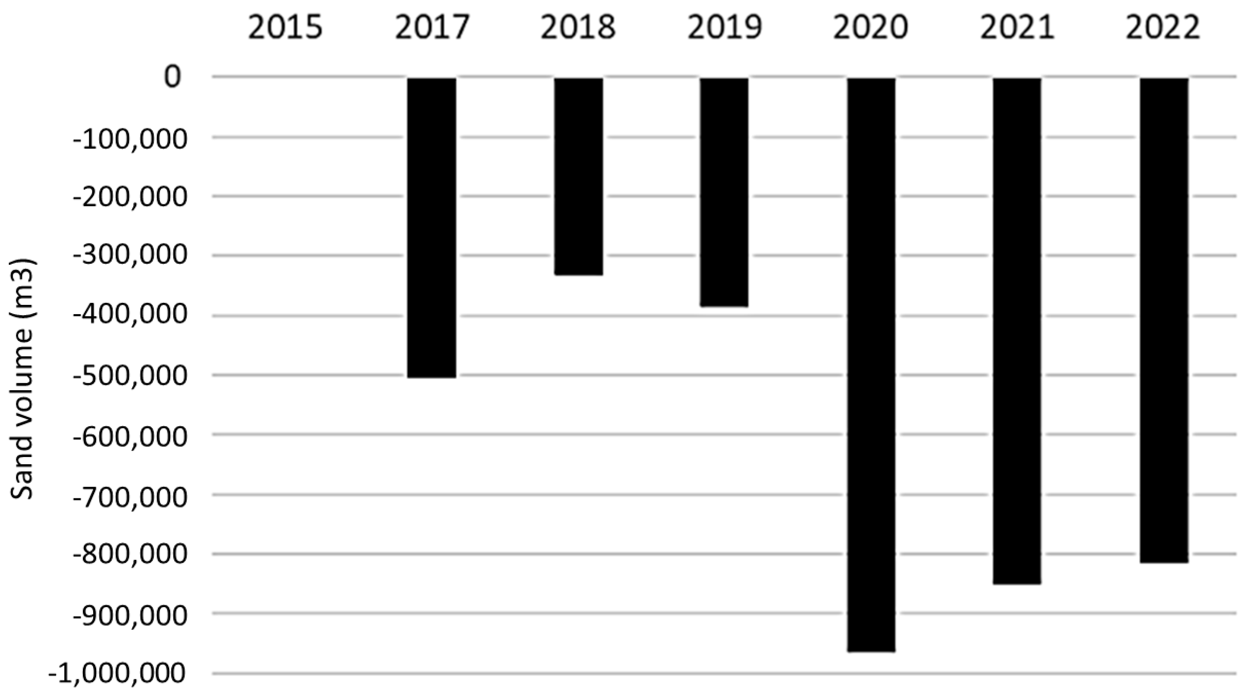
| Year | Total Volume (m3) | Differences with Respect to 2015 (m3) | Percentage of Change (%) |
|---|---|---|---|
| 2015 | 4,024,486.6 | 0.0 | 0.0 |
| 2017 | 3,521,001.5 | −503,485.1 | −12.5 |
| 2018 | 3,695,544.6 | −328,942.0 | −8.2 |
| 2019 | 3,640,938.1 | −383,548.4 | −9.5 |
| 2020 | 3,061,109.8 | −963,376.7 | −23.9 |
| 2021 | 3,175,796.8 | −848,689.8 | −21.1 |
| 2022 | 3,210,691.0 | −813,795.6 | −20.2 |
Disclaimer/Publisher’s Note: The statements, opinions and data contained in all publications are solely those of the individual author(s) and contributor(s) and not of MDPI and/or the editor(s). MDPI and/or the editor(s) disclaim responsibility for any injury to people or property resulting from any ideas, methods, instructions or products referred to in the content. |
© 2025 by the authors. Licensee MDPI, Basel, Switzerland. This article is an open access article distributed under the terms and conditions of the Creative Commons Attribution (CC BY) license (https://creativecommons.org/licenses/by/4.0/).
Share and Cite
Almonacid-Caballer, J.; Cabezas-Rabadán, C.; Gorkovchuk, D.; Palomar-Vázquez, J.; Pardo-Pascual, J.E. Re-Using Historical Aerial Imagery for Obtaining 3D Data of Beach-Dune Systems: A Novel Refinement Method for Producing Precise and Comparable DSMs. Remote Sens. 2025, 17, 594. https://doi.org/10.3390/rs17040594
Almonacid-Caballer J, Cabezas-Rabadán C, Gorkovchuk D, Palomar-Vázquez J, Pardo-Pascual JE. Re-Using Historical Aerial Imagery for Obtaining 3D Data of Beach-Dune Systems: A Novel Refinement Method for Producing Precise and Comparable DSMs. Remote Sensing. 2025; 17(4):594. https://doi.org/10.3390/rs17040594
Chicago/Turabian StyleAlmonacid-Caballer, Jaime, Carlos Cabezas-Rabadán, Denys Gorkovchuk, Jesús Palomar-Vázquez, and Josep E. Pardo-Pascual. 2025. "Re-Using Historical Aerial Imagery for Obtaining 3D Data of Beach-Dune Systems: A Novel Refinement Method for Producing Precise and Comparable DSMs" Remote Sensing 17, no. 4: 594. https://doi.org/10.3390/rs17040594
APA StyleAlmonacid-Caballer, J., Cabezas-Rabadán, C., Gorkovchuk, D., Palomar-Vázquez, J., & Pardo-Pascual, J. E. (2025). Re-Using Historical Aerial Imagery for Obtaining 3D Data of Beach-Dune Systems: A Novel Refinement Method for Producing Precise and Comparable DSMs. Remote Sensing, 17(4), 594. https://doi.org/10.3390/rs17040594