Research on 3D Reconstruction Methods for Incomplete Building Point Clouds Using Deep Learning and Geometric Primitives

Abstract

Point cloud data, known for their accuracy and ease of acquisition, are commonly used for reconstructing level of detail 2 (LoD-2) building models. However, factors like object occlusion can cause incompleteness, negatively impacting the reconstruction process. To address this challenge, this paper proposes a method for reconstructing LoD-2 building models from incomplete point clouds. We design a generative adversarial network model that incorporates geometric constraints. The generator utilizes a multilayer perceptron with a curvature attention mechanism to extract multi-resolution features from the input data and then generates the missing portions of the point cloud through fully connected layers. The discriminator iteratively refines the generator’s predictions using a loss function that is combined with plane-aware Chamfer distance. For model reconstruction, the proposed method extracts a set of candidate polygons from the point cloud and computes weights for each candidate polygon based on a weighted energy term tailored to building characteristics. The most suitable planes are retained to construct the LoD-2 building model. The performance of this method is validated through extensive comparisons with existing state-of-the-art methods, showing a 10.9% reduction in the fitting error of the reconstructed models, and real-world data are tested to evaluate the effectiveness of the method.

1. Introduction

Three-dimensional (3D) building models are essential components of digital cities, serving as fundamental elements and information carriers within these cities [1]. These models are constructed at various levels of detail (LoD), with LoD-2 models being particularly significant. LoD-2 models represent all the planes that form the model boundaries with relatively low detail. This allows them to meet the requirements of a building with moderate detail, making them suitable for spatial analysis [2] and enabling real-time rendering of large-scale scenes, which is crucial in urban environments. As a result, LoD-2 models are critical to 3D urban modeling [3]. Currently, the primary methods for constructing LoD-2 building models include manual modeling, photogrammetric modeling, and point-cloud-based modeling. Manual modeling relies on architectural drawings or satellite imagery but is labor-intensive and difficult to scale. Photogrammetric modeling, while efficient, is highly sensitive to environmental factors such as lighting, often resulting in lower model accuracy and quality. In contrast, point-cloud-based modeling offers high precision, accurately captures geometric shapes without requiring physical contact with objects, and exhibits strong adaptability to various environments. These advantages make point-cloud-based modeling particularly suitable for 3D building reconstruction and other reverse engineering applications.

However, during point cloud data acquisition, factors such as sensor quality, viewpoint limitations, and insufficient sampling density can often lead to incomplete building point clouds, which negatively affect the quality of subsequent building model reconstruction. As a result, generating high-quality building models from incomplete point clouds has become a critical and challenging task.

To address this challenge, this paper proposes a novel method for generating LoD-2 building models from incomplete point clouds. Generative Adversarial Networks (GANs), as a deep learning approach, have made significant progress in image generation and data completion in recent years. By training a generator and a discriminator in an adversarial manner, GANs generate highly realistic data. In the proposed method, GANs are first used to predict the missing portions of the building point cloud to produce a complete dataset. Next, it segments the point cloud into planes, generating a set of candidate polygons for model reconstruction. This method combines the strengths of GANs in predicting missing data with the advantages of geometric primitive-based reconstruction for generating lightweight, regularized models, offering an efficient solution for reconstructing building models from incomplete point clouds.

The main contributions of this work are as follows:

(1)

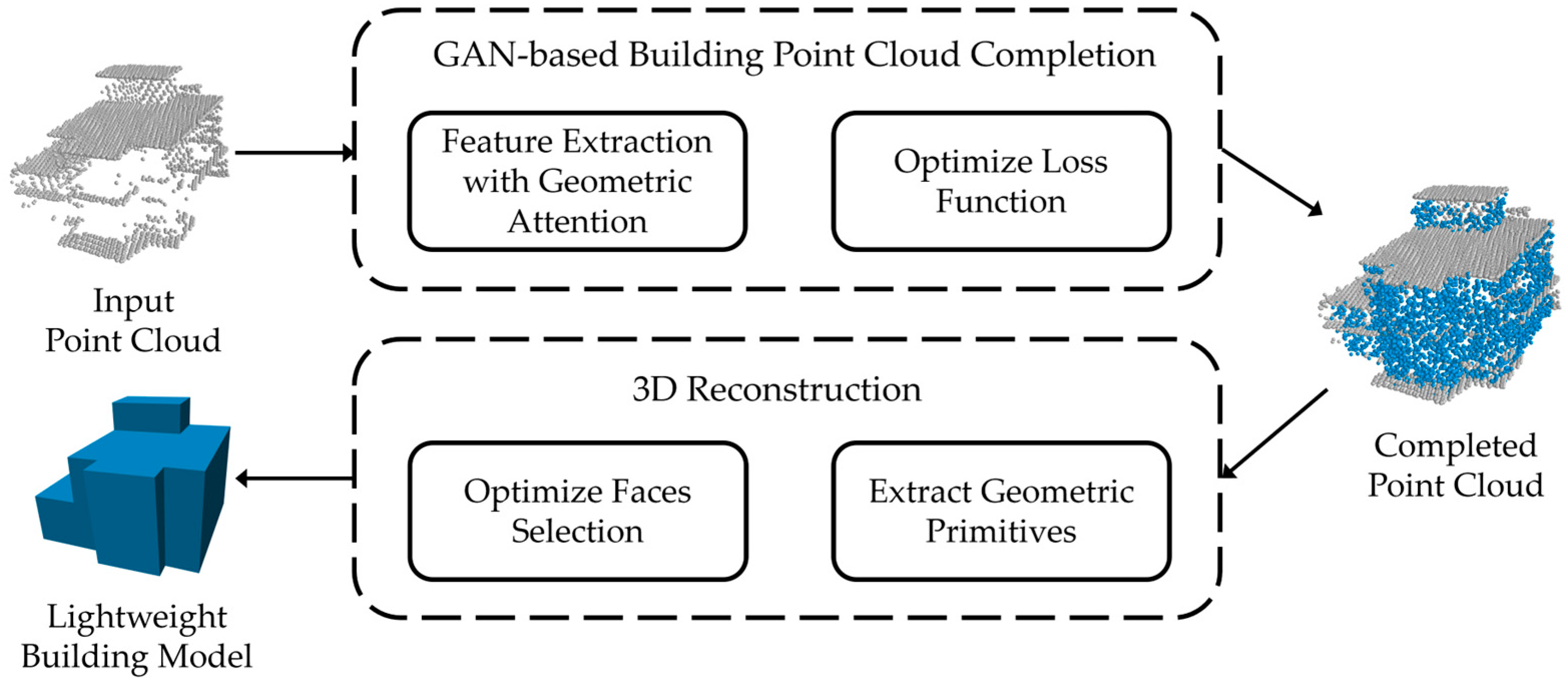
We propose a point cloud completion method tailored to building scenes. This method utilizes a multiscale feature fusion approach based on a GAN to complete missing building point cloud data. Geometric constraints are incorporated into both the feature extraction process and the loss function, significantly improving the accuracy of feature extraction and the prediction of missing regions.

(2)

A novel method for LoD-2 building model reconstruction is introduced, reformulating the task as a binary labeling problem. Planes extracted from the point cloud are segmented into candidate surfaces, and a weighted energy term, customized to building characteristics, is used to calculate the weight of each surface. Suitable surfaces are then selected to create a lightweight LoD-2 3D building model.

The rest of the paper is organized as follows: Section 2 introduces existing building point cloud reconstruction methods based on deep learning and geometric primitives, analyzing their limitations. Section 3 provides a detailed description of the proposed building point cloud completion and reconstruction method based on GAN and geometric constraints. Section 4 introduces the experimental setup and datasets, evaluating the performance of the proposed method. Section 5 summarizes the contributions of this paper and discusses future research directions.

2. Related Work

2.1. Point Cloud Completion

Traditional point cloud completion methods primarily rely on template matching [4,5,6] or geometric rule-based techniques [7,8,9] to interpolate and reconstruct missing regions, aiming to restore the complete shape of objects as accurately as possible. These methods are effective for handling small-scale missing data or point clouds with low noise. However, their performance significantly deteriorates when dealing with complex structures, sparse point clouds, or large-scale missing regions. As point cloud applications become more diverse and complex, the limitations of traditional methods become increasingly apparent. As a result, researchers have gradually turned to deep-learning-based approaches to improve both the accuracy and robustness of point cloud completion.

In contrast to traditional methods, deep-learning-based approaches do not rely on predefined handcrafted features. Instead, they can effectively leverage the rich shape information present in large-scale training datasets. Recently, researchers have extended convolutional neural networks (CNNs), widely used for two-dimensional (2D) image restoration, into 3D space by developing voxel-based 3D CNNs (3D-CNNs) for shape completion. For example, methods such as 3D-EPN [10] and GRNet [11] adopt a coarse-to-fine strategy to reconstruct 3D shapes. These approaches first use 3D-CNNs within an encoder–decoder framework to predict a coarse global structure, which is then refined by matching geometric constraints to shape databases, resulting in a completed 3D shape. Several other studies have also focused on shape inference and completion based on voxel data. For instance, Han et al. [12] used voxel data to simultaneously infer global structure and local geometric details, enabling high-resolution 3D shape completion. However, despite their high-quality feature learning, 3D-CNNs become computationally expensive as resolution increases, making them less efficient for handling fine geometric details.

To overcome these limitations, R.Q. Charles et al. [13] introduced PointNet, a network that enables deep learning to be directly applied to unstructured point cloud data. PointNet addresses the challenges of rotation invariance and unordered data in point clouds by incorporating affine transformations and symmetric functions. FoldingNet [14] further advanced this idea by introducing a “folding” operation that maps 2D features to 3D space for point cloud completion. PCN [15] applied the “folding” operation to generate smoother surfaces, while TopNet [16] proposed a tree-structured decoder to generate structure-aware point clouds. The self-attention mechanism of Transformer [17] can extract information in complex scenarios and has shown remarkable performance in semantic segmentation tasks [18]. ProxyFormer [19] introduced a proxy alignment-based method that uses a Transformer to predict and complete point cloud gaps, with sensitivity to missing regions. GAN-based point cloud completion methods have also garnered attention, as they are capable of generating missing point clouds that closely resemble real data distributions, significantly improving the accuracy and realism of point cloud reconstruction. PF-Net [20], based on a GAN architecture, proposed a multiresolution encoder-decoder framework that generates point clouds in a coarse-to-fine manner. RL-GAN-Net [21] combines GANs with reinforcement learning, achieving robust completion of point clouds with large missing regions. I-PAttnGAN [22] introduces a point cloud density attention mechanism, integrating prior information from image data to enhance the quality of point cloud generation in sparse regions. As point cloud completion techniques continue to evolve, these methods have been gradually applied to various domains. For instance, Ge et al. [23] applied them to trees, Wang et al. [24] to oil tanks, and Xia et al. [25] to vehicles.

However, most existing methods rely on a single global shape to predict the complete point cloud, which often presents challenges in preserving fine structural details. Additionally, these models are generally designed for general-purpose scenarios, whereas building point clouds possess unique geometric features and structures. Therefore, integrating architectural structural features with deep learning-based point cloud completion methods for building point cloud completion is the focus of this study.

2.2. Building Reconstruction from Point Cloud Data

Researchers have proposed several effective point-cloud-based 3D surface reconstruction methods, which can be broadly categorized into Delaunay triangulation, implicit surface reconstruction, and geometric primitive-based reconstruction.

Boissonnat et al. [26] were pioneers in applying Delaunay triangulation for 3D point-cloud-based surface reconstruction, focusing on discrete surface representation. Edelsbrunner et al. [27] introduced the α-shape algorithm, where the parameter α controls the level of detail in the reconstructed polyhedral model. However, selecting an appropriate value for α remains a challenging task. Benardin [28] proposed a method that identifies optimal points within spheres of a specified radius to determine mesh vertices, iteratively updating region boundaries to generate new triangles. Despite its effectiveness, choosing the correct radius for the spheres continues to pose a significant challenge.

Implicit surface reconstruction represents spatial boundaries using the isosurface of an implicit function. Carr et al. [29] used radial basis functions fitted to local point clouds and derived the zero-level isosurface as the reconstructed surface. The Poisson reconstruction algorithm [30] employs a hierarchy of locally supported basis functions and constrains the alignment of the implicit function gradient with point cloud normals, resulting in a global indicator function. This method is highly robust, effectively reconstructing irregularly shaped point clouds and compensating for small amounts of noise. It excels in repairing holes in reconstructed surfaces, producing smooth results, and offers advantages in mesh simplification and segmentation, making it a versatile tool for surface reconstruction.

While these methods extract surface features from point clouds to reconstruct 3D mesh models, the reconstruction process typically involves generating numerous surface patches through the construction of a triangular irregular network, which are then combined to create the final model. This approach often results in large data volumes, making it less suitable for large-scale urban building model reconstruction.

Geometric primitive-based reconstruction methods are well-suited for modeling objects with regular shapes. Schnabel et al. [31] introduced the RANSAC (random sample consensus) method, which robustly extracts geometric primitives such as cylinders and planes from point clouds. Building on this, several approaches [32,33] have explored decomposing point clouds and simultaneously fitting multiple geometric primitives, reducing the complexity and data volume of 3D models, thus improving processing and rendering efficiency. City3D [34] extracts roof planes of buildings through geometric primitive extraction and reconstructs building models by extruding walls based on building outline data, partially addressing the issue of missing data in building point clouds but losing significant wall details. Compared to other approaches, geometric primitive-based methods are particularly well-suited for reconstructing lightweight building models. However, incomplete point clouds or noise-induced points may be erroneously fitted as inaccurate planes, resulting in redundant or illogical surfaces within the building model. Therefore, generating LoD-2 models that more accurately reflect the structural characteristics of buildings from point clouds is another key focus of our research.

3. Method

The technical flow of the proposed method, as illustrated in Figure 1, primarily comprises two key components: point cloud completion and 3D reconstruction. Initially, the incomplete building point cloud is completed using a GAN model that incorporates geometric constraints and an optimized loss function. Subsequently, a candidate set of planes is extracted from the completed point cloud. Based on a geometric feature energy term, the most suitable planes are selected from this candidate set to construct a lightweight building model.

Figure 1. Technical flowchart of the proposed method, encompassing building point cloud completion and 3D reconstruction.

3.1. Completion of Missing Building Point Clouds Using GANs and Multiresolution Feature Fusion

GANs [35] have gained significant attention in point cloud completion tasks due to their strong performance in image generation and completion. This paper proposes a GAN-based method for completing incomplete building point clouds using multiresolution feature extraction. The detailed architecture of the proposed method is illustrated in Figure 2. We will elucidate the general workflow of the proposed method with reference to this figure. The method can be regarded as consisting of two primary components: the generator, which corresponds to the upper part of the diagram, and the discriminator, which corresponds to the lower part. Initially, the input point cloud data is downsampled to multiple resolutions, facilitating the extraction of both local and global latent features through a combined multi-layer perception (CMLP) module, which incorporates a set attention mechanism. These features, corresponding to different resolutions, are then concatenated into a unified feature vector. The combined vector is processed through two fully connected layers, generating the predicted point clouds in a coarse-to-fine manner. The discriminator evaluates the quality of the predicted point cloud by incorporating both a generation loss and a point cloud completion loss. Adversarial training is then applied, with the results backpropagated to improve the network’s ability to generate missing point clouds. The detailed architecture of the network and the specific implementation process of the algorithm will be further explained in subsequent sections.

Figure 2. Architecture of the proposed building point cloud completion model.

3.1.1. Multiresolution–Resolution Feature Extraction with Geometric Constraints

Building point cloud data typically exhibit complex geometric structures, with most buildings consisting of basic geometric shapes, such as planes. Therefore, effectively capturing these geometric features during point cloud feature extraction is essential for enhancing data representation and improving computational efficiency. This paper proposes a geometry-constrained multiresolution feature extraction method specifically designed for building point cloud data. By integrating farthest point sampling (FPS) [36] with a geometry-constrained attention mechanism, the method ensures that key geometric features are accurately captured and utilized during the extraction process.

The process begins by applying FPS to the original building point cloud data, creating two resolutions of point cloud datasets—a high-resolution dataset (N) and a low-resolution dataset (N/k)—as depicted in the initial section of the algorithm model architecture diagram presented in Figure 2. Features are then extracted separately from these two resolutions. To enhance the extraction of geometric features, particularly those related to planar structures, this paper introduces a curvature-based geometric attention mechanism. This mechanism dynamically adjusts feature extraction weights based on the curvature information of the building point cloud, enabling more accurate capture of the geometric features inherent in building structures. Curvature information plays a critical role in identifying edges, corners, and curved regions on the building surfaces. This mechanism directs the model’s attention to these areas with significant geometric variations, thereby assigning higher weights to these regions during feature extraction. As a result, the model can more accurately reconstruct the details of the building. By leveraging this approach, the curvature attention mechanism enhances the point cloud completion process, particularly when dealing with complex shapes and missing data, effectively reducing errors and improving reconstruction accuracy.

(1)

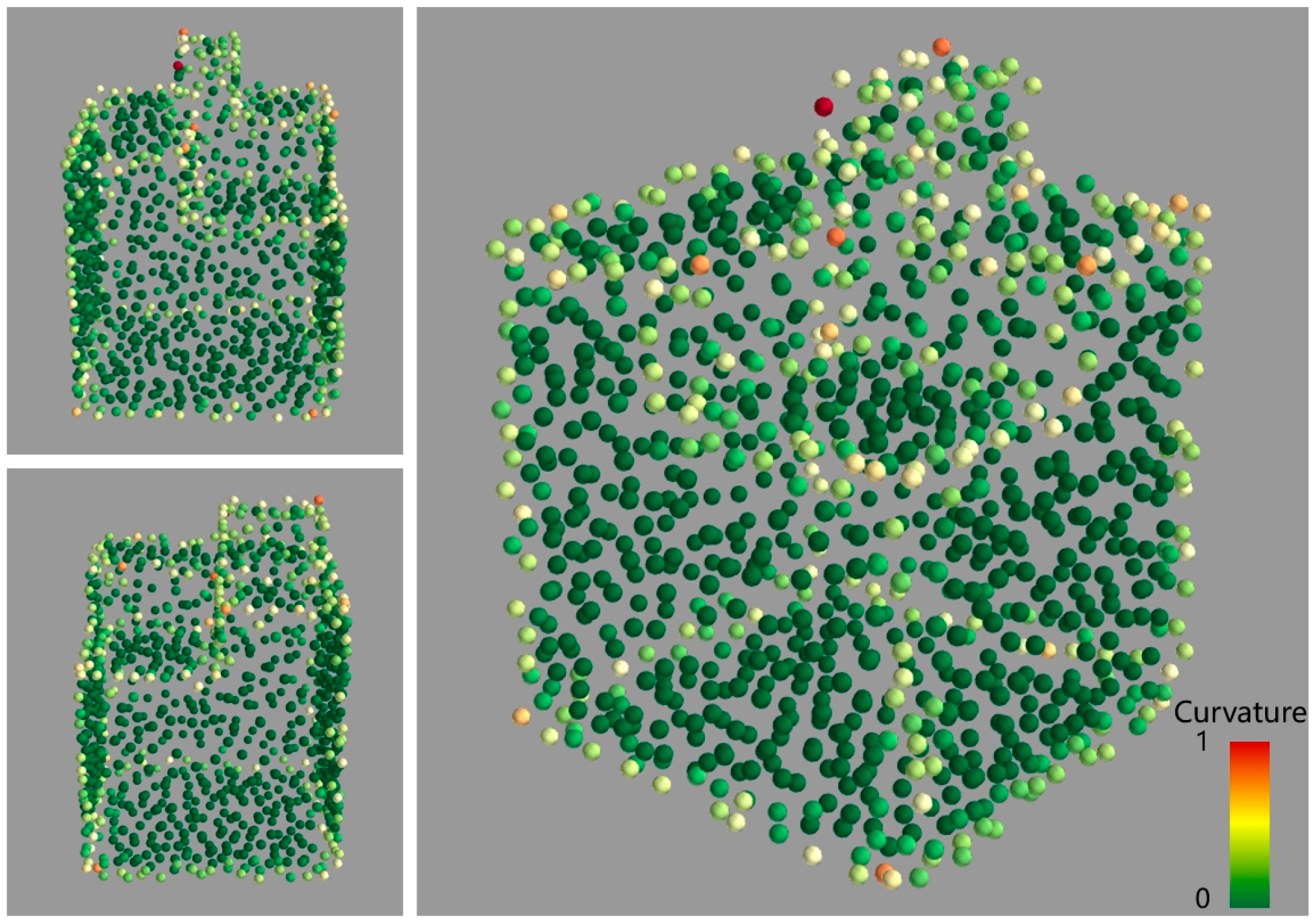
Curvature calculation for each point. For a sampled point $p_i$, its neighborhood point set $N\left(p_i\right)$ is determined using the k-nearest neighbors (KNN) method. The curvature ${\kappa }_i$ of point $p_i$ is then computed using principal component analysis [37]. The detailed process is outlined in Equations (1)–(3). Let the neighborhood points be $p_{i1},p_{i2}$, …, $p_{ik}$. First, the mean of the neighborhood points ${\overline{p}}_i$ is calculated as follows:

$${\overline{p}}_i={\displaystyle \frac{1}{k}}\sum _{j=1}^k{p}_{ij}$$

(1)

where $p_{ij}$ represents the coordinate vector of the $j$-th point in the neighborhood. Next, the covariance matrix $C_i$ is computed as follows:

$$C_i={\displaystyle \frac{1}{k}}\sum _{j=1}^k\left(p_{ij}-{\overline{p}}_i\right){\left(p_{ij}-{\overline{p}}_i\right)}^T$$

(2)

The covariance matrix $C$ undergoes eigenvalue decomposition, yielding three eigenvalues, ${\lambda }_{i1} \ge {\lambda }_{i2} \ge {\lambda }_{i3}$. The curvature ${\kappa }_i$ of point is then calculated using the following equation:

$${\kappa }_i={\displaystyle \frac{{\lambda }_{i3}}{{\lambda }_{i1}+{\lambda }_{i2}+{\lambda }_{i3}}}$$

(3)

Figure 3 visualizes the curvature values of each point in the building point cloud. Multiresolution feature extraction is highly effective for processing point cloud data with complex structures. By capturing both local and global features at different resolutions, the model can provide richer, more detailed information. The FPS method helps uniformly select representative points from the point cloud, effectively preserving the overall geometric structure while significantly reducing computational complexity.

Figure 3. Visualization of the curvature values in the point cloud.

(2)

Generating geometric attention weights. After computing the curvature values for each point, these values are combined with the point’s position and normal vector information as input data for feature extraction. The processed input data have a format of $N\times 4$, where $N$ is the number of sampled points, and the four dimensions include 3D position data and the one-dimensional curvature value. To allow the model to dynamically adjust its focus on individual points based on their curvature, attention weights for each point need to be generated. The attention weight ${\alpha }_i$ for each point is calculated from the curvature value ${\kappa }_i$ using Equation (4). To generate the attention weights, the curvature values are first normalized using the min–max scaling method. The normalized values are then passed through a multilayer perceptron (MLP), which generates the attention weights for each point based on its curvature.

$${\mathsf{\alpha }}_i=\sigma \left(W ·{\kappa }_i^{\prime }+b\right)$$

(4)

where $W$ is the weight matrix of the MLP that processes the curvature, $b$ is the bias term, and $\sigma \left(\right)$ represents the Gumbel–Softmax [38] function with a temperature parameter $\tau$, which normalizes the weights. ${\kappa }_i^{\prime }$ denotes the normalized curvature value. The calculation process is outlined in Algorithm 1 and can be expressed as follows.

Algorithm 1 Generating Geometric Attention Weights
Require: Point positions $P\in R^{N\times 3}$, curvature values $\kappa \in R^N$
Ensure: Attention weights ${\alpha }_i\in R^N$
1:	${\kappa }^{\prime }\leftarrow {\displaystyle \frac{\kappa -\min \left(\kappa \right)}{\max \left(\kappa \right)-\min \left(\kappa \right)}}$
2:	$F\leftarrow \mathrm{\varnothing }${Initialize feature matrix}
3:	for each point $i \in \{1, 2, \dots , N\}$ do
4:	$f_i\leftarrow \left[P_i,{\kappa }_i^{\prime }\right]$
5:	Append $f_i$ to $F$
6:	end for
7:	$Z\leftarrow W·F+b$
8:	${\alpha }_i\leftarrow \sigma \left(Z_i\right)\hspace{1em}\forall i\in \{1,2,\dots ,N\}$ {Apply Gumbel Softmax with temperature τ}
9:	return ${\alpha }_i$

(3)

Feature extraction. The complete process of feature extraction is illustrated in the upper part of Figure 2. In the feature extraction stage, an MLP is used to progressively increase the dimensionality of each point’s feature information, with dimensions of (64, 128, 256, 512, 1024). Unlike traditional approaches that extract global features from the last layer, this paper incorporates the CMLP mechanism from PF-Net [20] to retain and integrate features from multiple levels. For the last four layers of the MLP, the outputs are multiplied by the attention weight ${\alpha }_i$ and then subjected to max pooling, producing multidimensional feature vectors $f_i$ (with sizes $f_i=128,256,512,1024$ neurons for $i$ = 1, …, 4). These feature vectors are concatenated to form the final latent vector $F$, which combines both high-dimensional and low-dimensional features, resulting in a total dimensionality of 1920. Given that there are two resolutions of input data, two 1920-dimensional feature vectors are generated. These vectors are concatenated to create the final latent feature representation $M$. Finally, an additional MLP layer [1,2] integrates $M$ into the ultimate feature vector $V$.

3.1.2. Generation of Missing Point Cloud Regions

This paper draws on the concept of feature pyramid networks [39], utilizing fully connected layers to make multilevel predictions in a coarse-to-fine manner based on the final feature vector. This approach helps preserve both global and local geometric structure features. The process of multi-level prediction can be found in the right section of Figure 2. Specifically, two fully connected layers ${\mathrm{F}\mathrm{C}}_i$ (with sizes ${\mathrm{F}\mathrm{C}}_i=1024, 256$ neurons for $i$ = 1, 2) are used to process the final feature vector $V$ and predict the point clouds progressively. First, the coarse global point cloud $Y_{\mathrm{c}\mathrm{o}\mathrm{a}\mathrm{r}\mathrm{s}\mathrm{e}}$ is generated through ${\mathrm{F}\mathrm{C}}_2$. Then, using the offset vector obtained from ${\mathrm{F}\mathrm{C}}_1$, the fine point cloud $Y_{\mathrm{d}\mathrm{e}\mathrm{t}\mathrm{a}\mathrm{i}\mathrm{l}}$ is predicted by adjusting each point in the coarse point cloud to serve as the center. This process generates the missing point cloud, which integrates both local and global features. The point cloud generation process is detailed in Algorithm 2.

Algorithm 2 Two-Level Point Generation with Coarse and detail Layers
Require: Final feature vector $V$
Ensure: Two-layer point clouds $Y_{coarse},$ $Y_{detail}$
1:	$F{C}_{coarse}\leftarrow \mathit{FullyConnectedLayer}\left(V,256\right)$
2:	$F{C}_{detail}\leftarrow \mathit{FullyConnectedLayer}\left(V,1024\right)$
3:	$Y_{coarse}\leftarrow \mathit{GeneratePoints}\left(F{C}_{coarse},\mathit{num}\_\mathit{points}=128\right)$
4:	$Y_{\mathrm{detail}}\leftarrow Array\left[ \right]$
5:	for each point $p$ in $Y_{coarse}$ do
6:	$$\begin{gathered} detail\_points\leftarrow \mathit{GenerateRelativePoints}\left(F{C}_{detial}, \mathit{center}\_\mathit{point}= \\ p, \mathit{num}\_\mathit{points}=4\right) \end{gathered}$$
7:	Append $detail\_points$ to $Y_{detail}$
8:	end for
9:	return $Y_{coarse}$, $Y_{detail}$

Based on the principles of GANs, this paper incorporates a discriminator during training to distinguish between real and predicted data, feeding the discrimination results back into the neural network to improve the accuracy of incomplete point cloud predictions. The Chamfer distance (CD), introduced by Fan et al. [40], is permutation-invariant and computationally more efficient than methods such as Earth Mover’s Distance [20]. Given that planar structures dominate buildings, this paper extends the classical CD by introducing a plane-aware CD (PCD) loss term into the discriminator’s loss function, as shown in Figure 2. The PCD extends the classical CD by incorporating normal vector angle calculations, allowing for the consideration of the orientation and alignment of planar structures in building point clouds. This enables a more precise evaluation of point cloud reconstruction quality. Figure 4 illustrates the basic principle of PCD. The distance metric is modified from the distance between predicted points and real points (${\mathrm{d}\mathrm{i}\mathrm{s}\mathrm{t}}_{CD}$) to the distance between predicted points and the real plane (${\mathrm{d}\mathrm{i}\mathrm{s}\mathrm{t}}_{PCD}$). Compared to classical CD, PCD offers a better assessment of the similarity between two building point cloud datasets. The calculation of the PCD loss term $d_{\mathrm{P}\mathrm{C}\mathrm{D}}$ is given in Equations (5) and (6).

$$d_{\mathrm{P}\mathrm{C}\mathrm{D}}\left(P,Q\right)={\displaystyle \frac{1}{\left|P\right|}}\sum _{p\in P}\left[\underset{q\in Q}{\min }\left({\left|\left|p-q\right|\right|}^2·\left(1-\cos {\mathsf{\theta }}_{pq}\right)\right)\right]+{\displaystyle \frac{1}{\left|Q\right|}}\sum _{q\in Q}\left[\underset{p\in P}{\min }\left({\left|\left|q-p\right|\right|}^2·\left(1-\cos {\mathsf{\theta }}_{qp}\right)\right)\right]$$

(5)

$$\cos {\mathsf{\theta }}_{pq}={\displaystyle \frac{\left(p-q\right)·n_p}{\left|\left|p-q\right|\right|·\left|\left|n_p\right|\right|}}$$

(6)

Figure 4. Illustration of the PCD metric.

In Equation (5), $P=\left\{\right(p_1,n_1),(p_2,n_2),\dots ,(p_m,n_m\left)\right\}$ represents the real point cloud with normal vectors, where $p_i$ denotes the position and $n_i$ denotes the normal vector. $Q=\{q_1,q_2,\dots ,q_n\}$ represents the predicted point cloud, which contains only positional information. Because only $P$ includes normal vectors, it follows that $\mathrm{c}\mathrm{o}\mathrm{s}{\theta }_{qp}=\mathrm{c}\mathrm{o}\mathrm{s}{\theta }_{pq}$. By incorporating PCD, the method for assessing the similarity between the predicted and real point clouds shifts from point-to-point distances to point-to-plane distances. This adjustment provides more accurate evaluation results in building point cloud scenarios dominated by planar structures. As shown in Equation (7), the PCD loss is calculated separately for the detailed point cloud $Y_{\mathrm{d}\mathrm{e}\mathrm{t}\mathrm{a}\mathrm{i}\mathrm{l}}$ and the ground truth point cloud $Y_{\mathrm{g}\mathrm{t}}$, as well as for the coarse point cloud $Y_{\mathrm{c}\mathrm{o}\mathrm{a}\mathrm{r}\mathrm{s}\mathrm{e}}$ and the downsampled ground truth point cloud $Y_{\mathrm{g}\mathrm{t}}^{\prime }$, which is obtained by applying FPS to $Y_{\mathrm{g}\mathrm{t}}$ to match the scale of $Y_{\mathrm{c}\mathrm{o}\mathrm{a}\mathrm{r}\mathrm{s}\mathrm{e}}$. These combined losses form the point cloud completion loss $L_{\mathrm{c}\mathrm{o}\mathrm{m}}$.

$$L_{\mathrm{c}\mathrm{o}\mathrm{m}}=d_{\mathrm{P}\mathrm{C}\mathrm{D}1}\left(Y_{\mathrm{d}\mathrm{e}\mathrm{t}\mathrm{a}\mathrm{i}\mathrm{l}},Y_{\mathrm{g}\mathrm{t}}\right)+d_{\mathrm{P}\mathrm{C}\mathrm{D}2}\left(Y_{\mathrm{c}\mathrm{o}\mathrm{a}\mathrm{r}\mathrm{s}\mathrm{e}},Y_{\mathrm{g}\mathrm{t}}^{\prime }\right)$$

(7)

In addition to the point cloud completion loss, the loss function also includes an adversarial loss ($L_{\mathrm{a}\mathrm{d}\mathrm{v}}$), as shown in Equation (8). Here, $G\left(x\right)$ denotes the completed point cloud generated by the generator, and the discriminator $D\left(\right)$ computes the probability that the input point cloud is real, distinguishing between predicted and ground truth point clouds. The structure of the discriminator can be found in the lower part of Figure 2. The discriminator consists of sequential MLP layers, with layer counts and neuron numbers set to [64, 64, 128, 256]. A max pooling operation is applied to the output of the last MLP layer to extract a global feature vector $G$ of size 256. This vector is then processed by four additional fully connected layers (256 → 128 → 64 → 1) to reduce its dimensionality to a single scalar value. The result is passed through a sigmoid function to produce the classification output:

$$L_{adv}=\sum _{i=1}^S\mathit{log}\left(D\left(y_i\right)\right)+\sum _{i=1}^S\mathit{log}\left(1-D\left(G\left(x_i\right)\right)\right)$$

(8)

The final loss function $L$ in this paper can be expressed as follows:

$$L={\lambda }_{\mathrm{c}\mathrm{o}\mathrm{m}}{L}_{\mathrm{c}\mathrm{o}\mathrm{m}}+{\lambda }_{\mathrm{a}\mathrm{d}\mathrm{v}}{L}_{\mathrm{a}\mathrm{d}\mathrm{v}}$$

(9)

In Equation (9), ${\lambda }_{\mathrm{c}\mathrm{o}\mathrm{m}}$ and ${\lambda }_{\mathrm{a}\mathrm{d}\mathrm{v}}$ represent the weights for the point cloud completion loss and adversarial loss, respectively, with their sum equal to 1. The loss function is used for backpropagation and weight updates in the generator, guiding it to iteratively optimize the prediction of the generated point cloud. After sufficient training and model convergence, the proposed completion method demonstrates high effectiveness in accurately reconstructing the missing regions of building point cloud data.

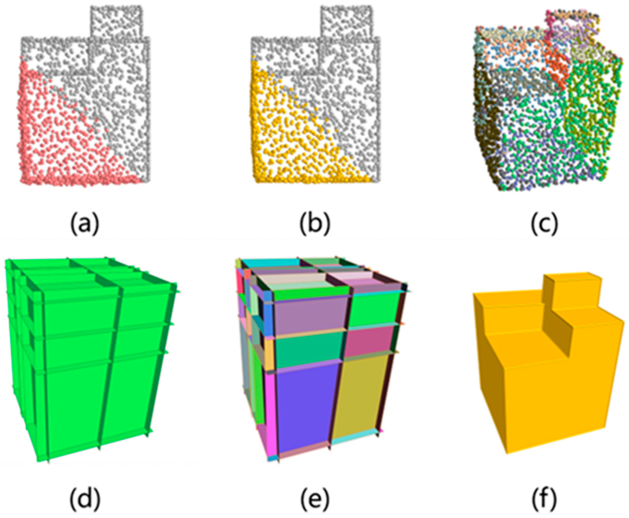
3.2. Three-Dimensional Surface Reconstruction of Buildings from Completed Point Clouds

By completing the missing regions of building point clouds, a nearly complete point cloud dataset of the building is obtained. Building on the PolyFit [41] algorithm, this paper formulates the reconstruction of building models as a binary labeling problem. Prior to model reconstruction, the point cloud is optimized using the moving least squares (MLS) method to minimize the impact of erroneous plane extractions. Next, planes are extracted from the point cloud using the RANSAC method and then segmented to form a candidate set of polygons. The most suitable polygons are selected by calculating weights based on a weighted energy function tailored to the specific features of building structures. This approach results in a watertight building model with a fully enclosed surface and no open boundaries. Figure 5 illustrates the workflow for 3D model reconstruction based on the completed point cloud.

Figure 5. Workflow of Building Model Reconstruction from Completed Point Clouds. (a) Completed point cloud data; (b) Point cloud optimized using Moving Least Squares to reduce discrete points; (c) Point cloud on the same plane calculated using RANSAC; (d) Generating individual planes from the point cloud and trimming the planes using bounding boxes; (e) Intersecting planes forming polygons; (f) Designing an energy equation to compute the most appropriate set of polygons, forming the 3D building model.

3.2.1. Point Cloud Optimization

Although the completed point cloud successfully reconstructs the overall structure of the missing parts of the building, it remains relatively scattered at the local level. This scattering can lead to the extraction of erroneous planes that do not align with the actual planes, resulting in inaccuracies in the final model structure. To address this issue, this study employs the MLS technique to fit planes by combining point cloud data with the original point cloud.

The point cloud data are divided into two parts: $P_{\mathrm{o}\mathrm{r}\mathrm{i}\mathrm{g}}=\{p_1,p_2,\dots ,p_n\}$ represents the original point cloud and $P_{\mathrm{c}\mathrm{o}\mathrm{m}\mathrm{p}}=p_1^{\prime },p_2^{\prime },\dots ,p_m^{\prime }$ represents the completed point cloud.

The combined point cloud, denoted as $P_{\mathrm{a}\mathrm{l}\mathrm{l}}$, are expressed as follows:

$${P_{\mathrm{a}\mathrm{l}\mathrm{l}}=P_{\mathrm{o}\mathrm{r}\mathrm{i}\mathrm{g}}\cup P}_{\mathrm{c}\mathrm{o}\mathrm{m}\mathrm{p}}$$

(10)

For each completed point $p_i^{\prime }\in P_{\mathrm{c}\mathrm{o}\mathrm{m}\mathrm{p}}$, its neighborhood points are selected from $P_{\mathrm{a}\mathrm{l}\mathrm{l}}$ using the KNN method:

$$\mathsf{{\rm N}}\left(p_i^{\prime }\right)=p_j\in P_{\mathrm{a}\mathrm{l}\mathrm{l}}:\mathrm{j}\in \mathrm{K}\mathrm{N}\mathrm{N}\left(p_i^{\prime },k\right)$$

(11)

where $\mathsf{{\rm N}}\left(p_i^{\prime }\right)$ represents the neighborhood point set of $p_i^{\prime }$, and $\mathrm{K}\mathrm{N}\mathrm{N}$ is the k-nearest neighbor function that returns the $k$ closest points to $p_i^{\prime }$. For each completed point $p_i^{\prime }$, the local plane is determined by minimizing the weighted least squares error, formulated as follows:

$$\underset{a,b,c,d}{\min }\sum _{q_i\in N\left(p_i^{\prime }\right)}w\left(p_i^{\prime },q_i\right)·{\left(a{q}_{i,x}+b{q}_{i,y}+c{q}_{i,z}+d\right)}^2$$

(12)

where $w\left(p_i^{\prime },q_i\right)$ is the weighting factor, defined as follows:

$$w\left(p_i^{\prime },q_i\right)=\mathrm{e}\mathrm{x}\mathrm{p}\left(-{\displaystyle \frac{{\left|\left|p_i^{\prime }-q_i\right|\right|}^2}{h^2}}\right)$$

(13)

where $q_i$ is a neighborhood point of $p_i^{\prime }$ and $q_i\in \mathsf{{\rm N}}\left(p_i^{\prime }\right)$; $h$ is the parameter controlling the decay of the weight; points closer to $p_i^{\prime }$ will have higher weights. The terms $q_{i,x}$, $q_{i,y}$, and $q_{i,z}$ represent the coordinates of the neighborhood point $q_i$. By solving the minimization problem in Equation (12), the plane parameters $a,b,c,d$ are obtained. The completed point $p_i^{\prime }$ is then projected onto the fitted local plane, yielding the optimized point $p_i^{″}$. The projection formula is as follows:

$$p_i^{″}=p_i^{\prime }-{\displaystyle \frac{a{p}_{i,x}^{\prime }+b{p}_{i,y}^{\prime }+c{p}_{i,z}^{\prime }+d}{a^2+b^2+c^2}}·\left(a,b,c\right)$$

(14)

where $p_{i,x}^{\prime }$, $p_{i,y}^{\prime }$, and $p_{i,z}^{\prime }$ represent the original coordinates of the completed point $p_i^{\prime }$. After plane optimization, the completed points become more coherent and smoother, as shown in Figure 5b.

3.2.2. Reconstruction of LoD-2 Building Models

Using the RANSAC method, planar information is extracted from the optimized point cloud (as shown in Figure 5c). Initially, the planes are preclipped using the bounding box of the point cloud, ensuring that the generated patches remain within the object’s region (as illustrated in Figure 5d). The processed planes are then intersected with each other, resulting in a set of N candidate polygons $F_i=\left\{F\right|1\le i\le N\}$ (as shown in Figure 5e). While this operation successfully segments the correct polygons, it also generates a significant number of redundant polygons. For example, as shown in Figure 6, a simple cube composed of six planes will produce correctly segmented green faces, as well as several extraneous yellow faces. To address this issue, redundant polygons are identified and removed in subsequent steps by evaluating their fit to the original point cloud data. Polygons with low fitting accuracy are discarded.

Figure 6. Generation of candidate polygons from point cloud data.

After obtaining the candidate polygon set $F_i$, a subset is selected that best represents the watertight geometric structure of the building. To achieve this, we define two energy terms—point fitting energy and building geometry feature energy—which together form the objective function for identifying the most appropriate polygons.

(1)

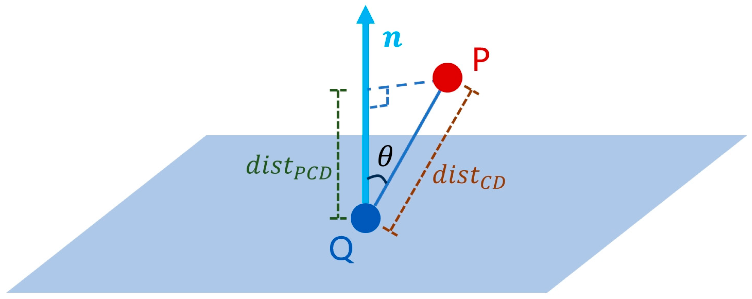
Point fitting. This energy term evaluates the degree of support that candidate polygons have from the input point cloud. It selects polygons that are well-aligned with the input point cloud and are supported by densely sampled regions [42]. The point fitting energy term $E_f$ is defined as follows:

$$E_f=1-{\displaystyle \frac{1}{\left|P\right|}}\sum _{i=1}^N{x}_i·\mathrm{s}\mathrm{u}\mathrm{p}\mathrm{p}\mathrm{o}\mathrm{r}\mathrm{t}\left(f_i\right)$$

(15)

$$\mathrm{s}\mathrm{u}\mathrm{p}\mathrm{p}\mathrm{o}\mathrm{r}\mathrm{t}\left(f_i\right)=\sum _{p\in P, \mathrm{d}\mathrm{i}\mathrm{s}\mathrm{t}\left(p, f_i\right)<\epsilon }\left(1-\left({\displaystyle \frac{\mathrm{d}\mathrm{i}\mathrm{s}\mathrm{t}\left(p, f_i\right)}{\epsilon }}\right)\right)·\mathrm{c}\mathrm{o}\mathrm{n}\mathrm{f}\left(p\right)$$

(16)

$$\mathrm{conf}\left(p\right)={\displaystyle \frac{1}{3}}\sum _{i=1}^3\left(1-{\displaystyle \frac{3{\mathsf{\lambda }}_1^i}{{\mathsf{\lambda }}_1^i+{\mathsf{\lambda }}_2^i+{\mathsf{\lambda }}_3^i}}\right)·{\displaystyle \frac{{\mathsf{\lambda }}_2^i}{{\mathsf{\lambda }}_3^i}}$$

(17)

where $\left|P\right|$ is the total number of points in $P$, and $N$ is the number of candidate polygons. The binary variable $x_i$ indicates whether the candidate polygon $f_i$ is selected. The term $\mathrm{s}\mathrm{u}\mathrm{p}\mathrm{p}\mathrm{o}\mathrm{r}\mathrm{t}\left(f_i\right)$ represents the weighted sum of points near the candidate polygon $f_i$, measuring its support. The term $\mathrm{d}\mathrm{i}\mathrm{s}\mathrm{t}\left(p,f_i\right)$ is the Euclidean distance between a point $p$ and the polygon $f_i$, with $ϵ$ being a distance threshold. The confidence term $\mathrm{c}\mathrm{o}\mathrm{n}\mathrm{f}\left(p\right)$ assesses the quality of the point cloud in the region around point $p$. Here, ${\lambda }_1^i\le {\lambda }_2^i\le {\lambda }_3^i$ are the three eigenvalues of the local covariance matrix of point $p$ at the $i$-th scale. The expression $1-3{\mathsf{\lambda }}_1^i/({\mathsf{\lambda }}_1^i+{\mathsf{\lambda }}_2^i+{\mathsf{\lambda }}_3^i)$ evaluates the quality of planar fitting in the local neighborhood, where values close to 1 indicate well-aligned points, and values close to 0 indicate a line or point cluster. The ratio ${\lambda }_2^i/{\lambda }_3^i$ measures the sampling uniformity of point $p$ in the local neighborhood, with values close to 1 indicating more uniform sampling.

(2)

Building geometry feature. This study focuses on general buildings, which are typically composed of vertical walls and horizontal roofs. To reconstruct models that better align with the structural characteristics of buildings, we introduce a building geometry feature energy term:

$$E_g=\sum _{i=1}^N{x}_i·\mathrm{v}\mathrm{e}\mathrm{r}\mathrm{t}\left(f_i\right)·\left(\mathrm{v}\mathrm{e}\mathrm{r}\mathrm{t}\left(f_i\right)-1\right)$$

(18)

$$\mathrm{v}\mathrm{e}\mathrm{r}\mathrm{t}\left(f_i\right)=1-\left|{\mathit{n}}_i·\mathit{z}\right|$$

(19)

In Equation (19), $\mathrm{v}\mathrm{e}\mathrm{r}\mathrm{t}\left(f_i\right)$ represents the degree of alignment of the $i$-th candidate plane $f_i$ with the vertical direction. Values closer to 0 indicate that the plane is near perfectly vertical, while values closer to 1 suggest that the plane is horizontal. Specifically, ${\mathit{n}}_i$ denotes the normal vector of $f_i$, and $\mathit{z}$ is the unit vector in the vertical direction. Intuitively, the building geometry feature term encourages the selection of planes that are either vertical or horizontal, reflecting the typical structural characteristics of buildings.

To ensure that the selected candidate polygons form a watertight model, these energy terms must be used under specific constraints. The necessary and sufficient condition for a watertight model is that each edge must be shared by exactly two polygons. Therefore, the candidate polygon selection is formulated as follows:

$$\underset{x}{\min }{\mathsf{\lambda }}_f·E_f+{\mathsf{\lambda }}_g·E_g$$

(20)

$$s.t.\left\{\begin{array}{cc}{\sum }_{j\in \mathcal{N}\left(e_i\right)}{x}_j=2 \mathrm{or} 0,& 1\le i\le \left|E\right|\hfill \\ x_i\in \{0,1\},& 1\le i\le N\hfill \end{array}\right.$$

(21)

In Equation (21), ${\sum }_{j\in \mathcal{N}\left(e_i\right)}{x}_j=2 \mathrm{or} 0$ ensures that each edge $e_i$ is shared by exactly two polygons or not selected at all. To solve this linear programming problem, we used the Gurobi solver [43]. The polygons selected with $x_i=1$ will form the watertight building model. This approach ensures the structural integrity of the reconstructed model by satisfying the necessary constraints for a watertight design.

4. Experiments

In this study, an LoD-2 building point cloud dataset was created to train the building point cloud completion model. The experiments were conducted on a Linux server equipped with dual RTX 2080 Ti GPUs (22 GB each) and an Intel Xeon Platinum 8336C CPU.

4.1. Building Point Cloud Dataset

This study used open-source 3D models of Adelaide, Australia [44], and building models from Longgang District, Shenzhen, China, as the original data. After manually removing low-quality models with missing faces, a filtered dataset of 2428 LoD-2 building models was compiled. The dataset includes a variety of building types, such as flat and sloped roofs, covering most common architectural structures. Point sampling was performed on each building model to create a point cloud representation, with an average of approximately 3000 points per model. The data format is ($x,y,z,n_x,n_y,n_z$), where the first three dimensions correspond to the position of a point, and the last three represent its normal vector. Each building point cloud was centered by aligning its centroid to the origin, and its coordinates were scaled and normalized to the range [−1, 1]. To simulate occlusions and missing data, we generated incomplete point clouds by randomly selecting a viewpoint and removing points closest to them.

4.2. Completion of Incomplete Building Point Clouds

The point cloud completion model was implemented using the PyTorch deep learning framework. The dataset was split into training, validation, and test subsets in a ratio of 8:1:1. During training, random batches from the training set were fed into the model. The ADAM optimizer was used for model training, with an initial learning rate of 0.0001, a weight decay of 0.001, and a batch size of 24. Each point cloud was downsampled to 2048 points (N), and the value of k was set to 8.

4.2.1. Quantitative Analysis for Point Cloud Completion

The proposed method was evaluated against four widely used point cloud completion algorithms—PCN [15], PF-Net [20], ShapeInversion(SI) [45] and SeedFormer [46]. Among these methods, PF-Net and ShapeInversion both utilize the GAN framework. To ensure a fair and consistent comparison, all algorithms were trained and tested on the same dataset. Given that the dataset does not contain labeled ground truth information, completion performance was assessed using two metrics: prediction-to-ground-truth error (Pre_Gt) [47] and ground-truth-to-prediction error (Gt_Pre) [48]. Pre_Gt measures the squared Euclidean distance between each predicted point and its nearest counterpart in the ground truth point cloud, indicating the deviation between the predicted and actual data. In contrast, Gt_Pre calculates the squared Euclidean distance from each ground truth point to its nearest neighbor in the predicted point cloud, quantifying how well the predicted shape represents the ground truth data. The sum of Pre_Gt and Gt_Pre gives the CD. The results of these metrics are presented in Table 1.

Table 1. Point cloud completion results for different methods. The values are scaled by a factor of 1000, with smaller values indicating higher similarity.

	PCN	PF-Net	SI	SeedFormer	Ours
Gt_Pre	0.976	0.740	0.573	0.436	0.508
Pre_Gt	1.181	0.504	0.635	0.633	0.404
CD	2.157	1.245	1.208	1.069	0.912

The results show that the proposed point cloud completion method achieved the lowest error on the building dataset, highlighting its effectiveness in completing incomplete building point clouds, particularly in LoD-2 scenarios characterized by planar structures.

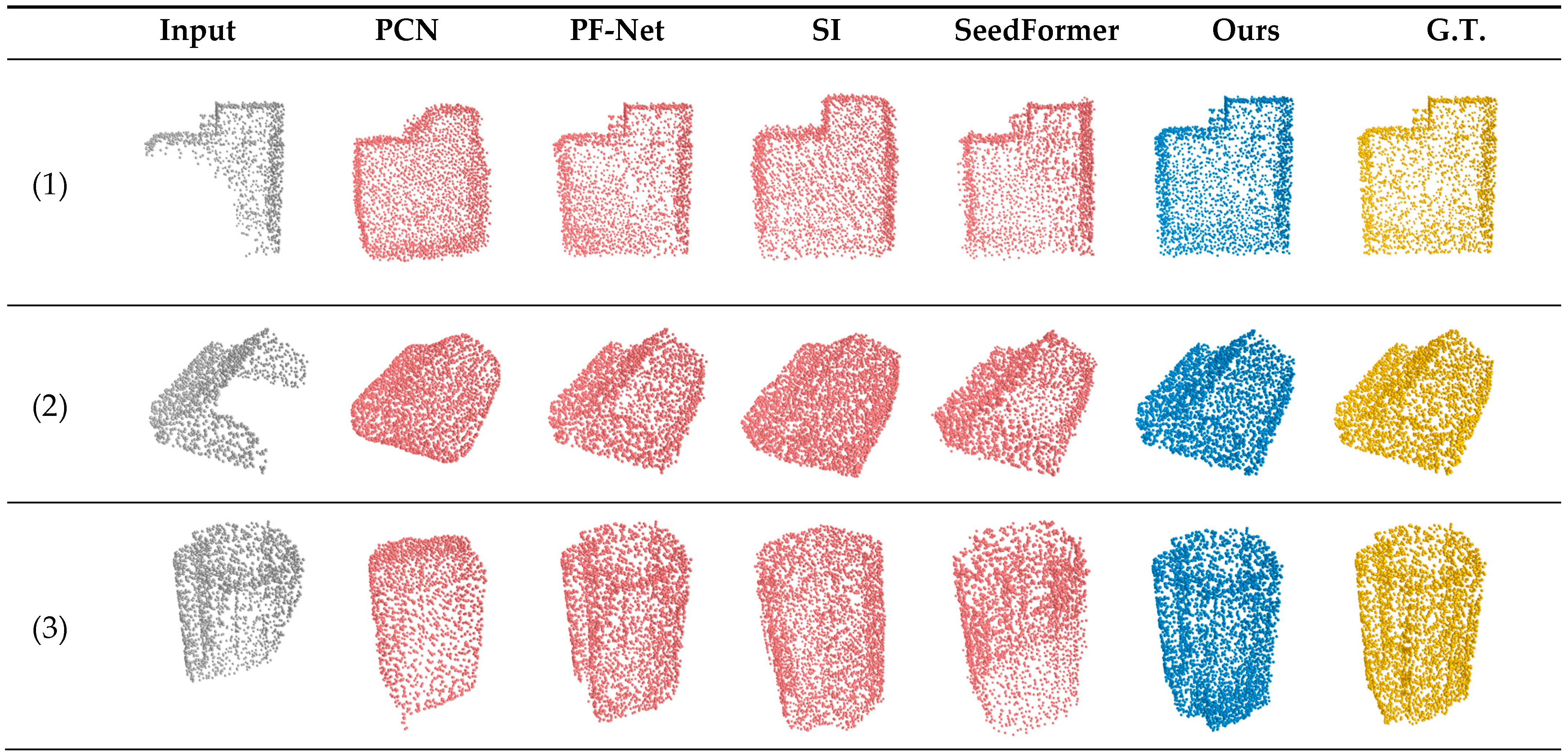
4.2.2. Qualitative Analysis for Point Cloud Completion

The building point cloud dataset was used to visualize the results of the proposed method in comparison with the widely adopted PCN [15], PF-Net [20], ShapeInversion and SeedFormer [46] approaches, as shown in Figure 7. The visualized results reveal that the proposed model outperforms the alternatives in detail completion. For instance, in building (2), PCN focuses on generating smooth surfaces but fails to preserve the sharp features of the buildings. Similarly, ShapeInversion completes the overall shape of the point cloud but loses some details. PF-Net reconstructs the main missing regions of the point cloud but leaves the edges relatively scattered. SeedFormer introduces many noise points while recovering the building. In contrast, the proposed method produces clearer, more defined edges, achieving superior completion in complex regions. Notably, in the lower section of building (3), the results from the proposed method are more aligned with the ground truth than those from the other approaches. These observations highlight the effectiveness of the proposed method in delivering high-quality point cloud completion, with better preservation of intricate geometric details.

Figure 7. Visualization of Point Cloud Completion Results for Building Models. (1), (2), and (3) represent different buildings used in this experiment.

4.2.3. Robustness Testing

In this section, we evaluated the robustness of the building point cloud completion model from two perspectives: the proportion of missing data and the number of missing regions. In the first test, we varied the proportion of missing data by adjusting the value of $M$ in the generator, and the results are visualized in Figure 8a, where 25%, 50%, and 75% represent the proportions of missing data relative to the original point cloud. The visualizations show that the completion results of our model align well with the ground truth across all three missing data levels. This indicates that the proposed model exhibits strong robustness in handling point clouds with varying amounts of missing data. In the second test, the model was applied to building point clouds with multiple missing regions. Partial results are presented in Figure 8b. The results demonstrate the model’s ability to identify different missing regions and accurately predict the missing data, further underscoring its effectiveness and robustness in more complex scenarios.

Figure 8. Results of robustness experiments. Blue points represent the completion results, and gray points represent the input data. (a) Completion results for different levels of missing data. 25%, 50%, and 75% indicate the proportion of missing parts relative to the ground truth data (G.T.). (b) Completion results for point clouds with multiple missing regions.

4.3. Building Model Reconstruction Experiments

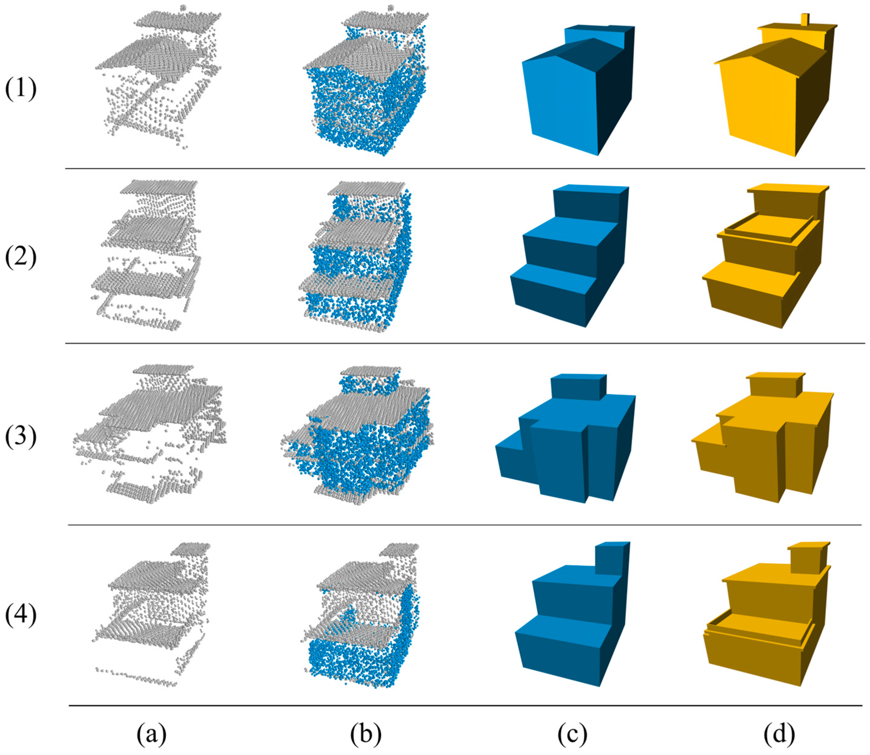
4.3.1. Qualitative Analysis for Reconstruction

To evaluate the proposed building surface reconstruction method, the completed building point cloud data were used to reconstruct 3D models using both existing surface reconstruction methods and the proposed method. Partial reconstruction results are shown in Figure 9, where the baseline model (G.T.) refers to the original building model used during the point cloud sampling process in the dataset creation.

Figure 9. Comparison of LoD-2 building model reconstruction results. (1), (2), and (3) represent different buildings used in this experiment.

This study presents a comparative analysis of the proposed method with the widely adopted PolyFit [41] and City3D [34] methods. PolyFit is a classic structural modeling method, while City3D reconstructs lightweight building models by extracting roof structure primitives and combining them with building footprints. Considering that triangular mesh modeling techniques tend to generate an excessive number of faces, resulting in overly detailed models that do not meet the lightweight requirements of LoD-2 building models, these methods were excluded from the comparative experiments. The experimental results show that all three methods are capable of successfully reconstructing building models from point cloud data. The PolyFit method computes all planes from the point cloud data and intersects them pairwise to generate candidate planes. After selecting closed surfaces, it produces lightweight models. However, this method is highly sensitive to noise and requires high accuracy in the point cloud data. When the point cloud is sparse, erroneous planes extracted from noisy data can degrade the quality of the final model. For instance, in Figure 9, Model 1—the red-boxed area, which should be a vertical plane—is incorrectly reconstructed as a slanted surface due to the influence of erroneous planes. Similar issues are observed in other models as well. The City3D method first extracts the roof structure and then generates the building model by combining vertical walls and horizontal ground derived from building footprints. This can lead to incorrect roof structures being extracted when the roof of the building is complex, which in turn affects the overall reconstruction quality, as seen in Model 3 in Figure 9. In contrast, the proposed method performs better in the same area, accurately reconstructing the vertical plane and avoiding the generation of slanted surfaces. This is because, unlike PolyFit, the proposed method prioritizes vertical and horizontal planes, reducing the impact of erroneous planes and producing models that better align with reality. Additionally, in Figure 9, Model 3, all three methods fail to accurately capture the curved surface of the real model, instead fitting planes to approximate it. This limitation arises from the fact that all three methods rely on plane extraction for reconstruction. However, the proposed method still outperforms PolyFit and City3D, generating results that are closer to the ground truth.

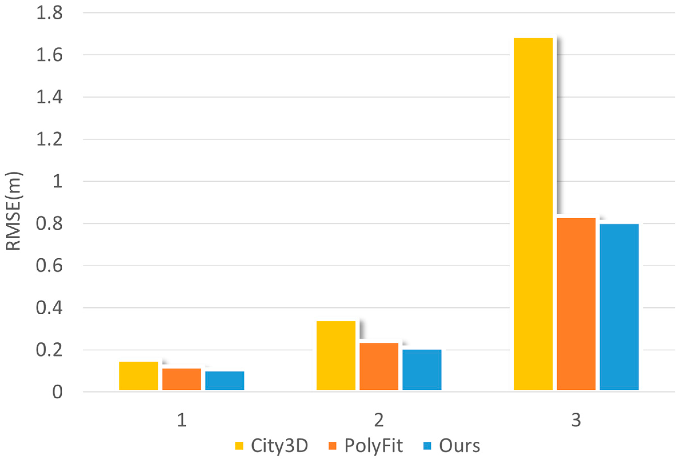
4.3.2. Quantitative Analysis for Reconstruction

This section uses the root mean square error as a metric of quantifying the similarity between the reconstructed models and the ground truth models. The results, shown in Figure 10, indicate that City3D loses more building details during reconstruction, especially in the wall areas, leading to higher errors compared to the other two methods. Compared to PolyFit, which has smaller errors, the proposed method consistently outperforms it, achieving an average error reduction of 10.9%. This improvement can be attributed to PolyFit’s tendency to generate models that closely fit the input point cloud. However, when dealing with sparse or noisy data, this often results in the inclusion of erroneous planes, causing larger discrepancies from the ground truth. In contrast, the proposed method is better able to disregard these erroneous planes, leading to more accurate and realistic reconstructions. Model 3, which contains curved walls, exhibits a higher overall error compared to other models. Both the proposed method and PolyFit introduce errors when approximating the curved surfaces with multiple planar primitives. However, even in this case, the proposed method delivers better performance than PolyFit. These experiments demonstrate that the proposed reconstruction method not only achieves higher accuracy but also produces more realistic models, making it a more suitable approach for LoD-2 building reconstruction from incomplete point clouds.

Figure 10. Quantitative comparison of model reconstruction results.

We also compared the reconstruction time of each method to evaluate efficiency. Table 2 presents the runtime and the total number of faces in the reconstructed models. City3D has a significantly increased running time compared to other methods due to the need to compute the pairwise intersection between detected planes and inferred vertical planes, which generates a large number of candidate faces. Although the total number of faces in its reconstructed model is the smallest, this also leads to the loss of certain building structures. Our method takes slightly longer than the fastest PolyFit, but the total number of faces is smaller. This is reflected in the model reconstruction where some erroneous planes are removed, producing a higher quality model, as can be verified by Figure 9.

Table 2. Comparison of reconstruction efficiency between City3D, PolyFit, and our method. Total face numbers and running times are reported.

Building in Figure 9	Method	Faces	Time (s)
1	City3D	8	10.63
	PolyFit	9	4.52
	Ours	8	5.18
2	City3D	8	16.24
	PolyFit	16	6.82
	Ours	11	7.96
3	City3D	18	28.91
	PolyFit	33	10.79
	Ours	25	13.27

4.4. Complex Data Testing

We further tested the effectiveness of our method on real-world building point cloud data with missing parts, where the test data were obtained by scanning with a LiDAR-equipped drone. Real-world data are often more complex than training data, with complexities such as sparse point clouds, irregular occlusions, and noise. We used the building point clouds, simply segmented from the drone-scanned data, as input and applied our method for point cloud completion and 3D reconstruction. The reconstruction results were compared with manually reconstructed building models, as shown in Figure 11. The results demonstrate that our method can complete incomplete building point clouds and perform lightweight building model reconstruction. However, there are some instances where reconstruction deviates. For example, in Building 4, due to the scarcity of point cloud data on the lower-left roof edge of the input, our reconstruction did not capture the protruding wall. Additionally, our method struggles with accurately reconstructing eaves. Despite these issues, our method successfully completed the 3D reconstruction of the buildings, with the reconstruction results being overall very similar to the manually reconstructed models.

Figure 11. Three-dimensional reconstruction results of complex scenes. (a) Input data: incomplete building point cloud data captured by a drone; (b) point cloud completion results: blue points represent the generated point cloud; (c) results of 3D reconstruction; (d) results from manual modeling. (1), (2), (3), and (4) represent different real-world buildings with incomplete point clouds.

5. Conclusions

This study presents a method for reconstructing LoD-2 building models from incomplete point clouds. We design a generative adversarial network model, incorporating geometric constraints, to predict the missing portions of building point clouds based on structural features. A curvature attention mechanism is introduced in the generator to extract multi-resolution features of the building, while the plane-aware Chamfer distance is utilized in the discriminator’s loss function to more precisely assess the prediction quality. For model reconstruction, the proposed method employs an energy equation aligned with building characteristics, selecting the most suitable planes from those extracted from the completed point cloud to construct the LoD-2 building model. The approach combines deep learning with geometric constraints to effectively complete building point clouds with missing data, which may arise due to various objective limitations. Compared to the PolyFit method and City3D method, the proposed 3D reconstruction method demonstrates superior performance in reconstructing LoD-2 models from completed point clouds. The experimental results confirm the effectiveness of the proposed method, offering a promising solution for 3D model reconstruction from incomplete building point clouds.

However, the method has some limitations. The input point cloud data is required to be of individual buildings, which necessitates additional building extraction and denoising when dealing with large-scale building data. Furthermore, the method primarily focuses on planar structures, and when applied to buildings with curved surfaces, it may struggle to extract sufficient information, leading to inaccurate reconstructions. Future work will explore the integration of techniques for recognizing and extracting incomplete individual buildings and feature extraction for regular curved surfaces, enabling automatic processing of large-scale data and reconstruction of non-planar structures from incomplete point clouds, thus expanding the applicability of the method.

References

1. Peters, R.; Dukai, B.; Vitalis, S.; van Liempt, J.; Stoter, J. Automated 3D reconstruction of LoD2 and LoD1 models for all 10 million buildings of the Netherlands. Photogramm. Eng. Remote Sens. 2022, 88, 165–170. [Google Scholar] [CrossRef]
2. Dehbi, Y.; Henn, A.; Gröger, G.; Stroh, V.; Plümer, L. Robust and fast reconstruction of complex roofs with active sampling from 3D point clouds. Trans. GIS 2021, 25, 112–133. [Google Scholar] [CrossRef]
3. Wang, F.; Zhou, G.; Hu, H.; Wang, Y.; Fu, B.; Li, S.; Xie, J. Reconstruction of LoD-2 Building Models Guided by Façade Structures from Oblique Photogrammetric Point Cloud. Remote Sens. 2023, 15, 400. [Google Scholar] [CrossRef]
4. Kim, V.G.; Li, W.; Mitra, N.J.; Chaudhuri, S.; DiVerdi, S.; Funkhouser, T. Learning part-based templates from large collections of 3D shapes. ACM Trans. Graph. 2013, 32, 1–12. [Google Scholar] [CrossRef]
5. Li, Y.; Dai, A.; Guibas, L.; Nießner, M. Database-assisted object retrieval for real-time 3D reconstruction. In Computer Graphics Forum; Wiley Online Library: Hoboken, NJ, USA, 2015; Volume 34, pp. 435–446. [Google Scholar]
6. Nan, L.; Xie, K.; Sharf, A. A search-classify approach for cluttered indoor scene understanding. ACM Trans. Graph. 2012, 31, 1–10. [Google Scholar] [CrossRef]
7. Mitra, N.J.; Pauly, M.; Wand, M.; Ceylan, D. Symmetry in 3D Geometry: Extraction and Applications. Comput. Graph. Forum 2013, 32, 1–23. [Google Scholar] [CrossRef]
8. Pauly, M.; Mitra, N.J.; Wallner, J.; Pottmann, H.; Guibas, L.J. Discovering structural regularity in 3D geometry. In ACM SIGGRAPH 2008 Papers; ACM: New York, NY, USA, 2008; pp. 1–11. [Google Scholar]
9. Zhao, W.; Gao, S.; Lin, H. A robust hole filling algorithm for triangular mesh. Vis. Comput. 2007, 23, 987–997. [Google Scholar] [CrossRef]
10. Dai, A.; Ruizhongtai Ci, C.; Nießner, M. Shape completion using 3D-encoder-predictor CNNs and shape synthesis. In Proceedings of the IEEE Conference on Computer Vision and Pattern Recognition, Honolulu, HI, USA, 21–26 July 2017; pp. 5868–5877. [Google Scholar]
11. Xie, H.; Yao, H.; Zhou, S.; Mao, J.; Zhang, S.; Sun, W. GRNet: Gridding Residual Network for Dense Point Cloud Completion. In Computer Vision—ECCV 2020; Vedaldi, A., Bischof, H., Brox, T., Frahm, J.M., Eds.; Lecture Notes in Computer Science; Springer: Cham, Switzerland, 2020; Volume 12354, pp. 581–597. [Google Scholar]
12. Han, X.; Li, Z.; Huang, H.; Kalogerakis, E.; Yu, Y. High-resolution shape completion using deep neural networks for global structure and local geometry inference. In Proceedings of the IEEE International Conference on Computer Vision, Venice, Italy, 22–29 October 2017; pp. 85–93. [Google Scholar]
13. Charles, R.Q.; Su, H.; Kaichun, M.; Guibas, L.J. PointNet: Deep Learning on Point Sets for 3D Classification and Segmentation. In Proceedings of the IEEE Conference on Computer Vision and Pattern Recognition (CVPR), Honolulu, HI, USA, 21–26 July 2017; pp. 77–85. [Google Scholar]
14. Yang, Y.; Feng, C.; Shen, Y.; Tian, D. FoldingNet: Point Cloud Auto-Encoder via Deep Grid Deformation. In Proceedings of the 2018 IEEE/CVF Conference on Computer Vision and Pattern Recognition (CVPR), Salt Lake City, UT, USA, 18–23 June 2018; pp. 206–215. [Google Scholar]
15. Yuan, W.; Khot, T.; Held, D.; Mertz, C.; Hebert, M. PCN: Point Completion Network. In Proceedings of the 2018 International Conference on 3D Vision (3DV), Verona, Italy, 5–8 September 2018; pp. 728–737. [Google Scholar]
16. Tchapmi, L.P.; Kosaraju, V.; Rezatofighi, H.; Reid, I.; Savarese, S. TopNet: Structural point cloud decoder. In Proceedings of the IEEE Conference on Computer Vision and Pattern Recognition (CVPR), Long Beach, CA, USA, 15–20 June 2019; pp. 383–392. [Google Scholar]
17. Vaswani, A. Attention is all you need. In Advances in Neural Information Processing Systems; MIT Press: Cambridge, MA, USA, 2017; Volume 30, pp. 5998–6008. [Google Scholar]
18. Chen, Y.; Zhou, J.; Ge, Y.; Dong, J. Uncovering the rapid expansion of photovoltaic power plants in China from 2010 to 2022 using satellite data and deep learning. Remote Sens. Environ. 2024, 305, 114100. [Google Scholar] [CrossRef]
19. Li, S.; Gao, P.; Tan, X.; Wei, M. Proxyformer: Proxy alignment assisted point cloud completion with missing part sensitive transformer. In Proceedings of the IEEE/CVF Conference on Computer Vision and Pattern Recognition (CVPR), Vancouver, BC, Canada, 17–24 June 2023; pp. 9466–9475. [Google Scholar]
20. Huang, Z.; Yu, Y.; Xu, J.; Ni, F.; Le, X. PF-Net: Point Fractal Network for 3D Point Cloud Completion. In Proceedings of the IEEE/CVF Conference on Computer Vision and Pattern Recognition (CVPR), Seattle, WA, USA, 13–19 June 2020; pp. 7662–7670. [Google Scholar]
21. Sarmad, M.; Lee, H.J.; Kim, Y.M. RL-GAN-Net: A Reinforcement Learning Agent Controlled GAN Network for Real-Time Point Cloud Shape Completion. In Proceedings of the IEEE/CVF Conference on Computer Vision and Pattern Recognition (CVPR), Long Beach, CA, USA, 15–20 June 2019; pp. 5898–5907. [Google Scholar]
22. Li, W.; Chen, Y.; Fan, Q.; Yang, M.; Guo, B.; Yu, Z. I-PAttnGAN: An Image-Assisted Point Cloud Generation Method Based on Attention Generative Adversarial Network. Remote Sens. 2025, 17, 153. [Google Scholar] [CrossRef]
23. Ge, B.; Chen, S.; He, W.; Qiang, X.; Li, J.; Teng, G.; Huang, F. Tree Completion Net: A Novel Vegetation Point Clouds Completion Model Based on Deep Learning. Remote Sens. 2024, 16, 3763. [Google Scholar] [CrossRef]
24. Wang, Y.; Liu, Y.; Zeng, H.; Zhu, H. Volume Estimation of Oil Tanks Based on 3D Point Cloud Completion. IEEE Trans. Instrum. Meas. 2024, 73, 2532810. [Google Scholar]
25. Xia, Y.; Xu, Y.; Wang, C.; Stilla, U. VPC-Net: Completion of 3D Vehicles from MLS Point Clouds. ISPRS J. Photogramm. Remote Sens. 2021, 174, 166–181. [Google Scholar] [CrossRef]
26. Boissonnat, J.-D. Geometric structures for three-dimensional shape representation. ACM Trans. Graph. 1984, 3, 266–286. [Google Scholar] [CrossRef]
27. Edelsbrunner, H.; Mücke, E.P. Three-dimensional alpha shapes. ACM Trans. Graph. 1994, 13, 43–72. [Google Scholar] [CrossRef]
28. Bernardini, F.; Mittleman, J.; Rushmeier, H.; Silva, C.; Taubin, G. The ball-pivoting algorithm for surface reconstruction. IEEE Trans. Vis. Comput. Graph. 1999, 5, 349–359. [Google Scholar] [CrossRef]
29. Carr, J.C.; Beatson, R.K.; Cherrie, J.B.; Mitchell, T.J.; Fright, W.R.; McCallum, B.C.; Evans, T.R. Reconstruction and representation of 3D objects with radial basis functions. In Proceedings of the 28th Annual Conference on Computer Graphics and Interactive Techniques (SIGGRAPH), Los Angeles, CA, USA, 12–17 August 2001; pp. 67–76. [Google Scholar]
30. Kazhdan, M.; Bolitho, M.; Hoppe, H. Poisson surface reconstruction. In Proceedings of the Fourth Eurographics Symposium on Geometry Processing (SGP ‘06), Sardinia, Italy, 26–28 June 2006; Eurographics Association: Goslar, Germany, 2006; pp. 61–70. [Google Scholar]
31. Schnabel, R.; Wahl, R.; Klein, R. Efficient RANSAC for Point-Cloud Shape Detection. Comput. Graph. Forum 2007, 26, 214–226. [Google Scholar] [CrossRef]
32. Li, M.; Nan, L.; Smith, N.G.; Wonka, P. Reconstructing building mass models from UAV images. Comput. Graph. 2016, 54, 84–93. [Google Scholar] [CrossRef]
33. Lin, H.C.; Gao, J.; Zhou, Y.; Lu, G.; Ye, M.; Zhang, C.; Liu, L.; Yang, R. Semantic Decomposition and Reconstruction of Residential Scenes from LiDAR Data. ACM Trans. Graph. 2013, 32, 66. [Google Scholar] [CrossRef]
34. Huang, J.; Stoter, J.; Peters, R.; Nan, L. City3D: Large-Scale Building Reconstruction from Airborne LiDAR Point Clouds. Remote Sens. 2022, 14, 2254. [Google Scholar] [CrossRef]
35. Goodfellow, I.; Pouget-Abadie, J.; Mirza, M.; Xu, B.; Warde-Farley, D.; Ozair, S.; Courville, A.; Bengio, Y. Generative adversarial networks. Commun. ACM 2020, 63, 139–144. [Google Scholar] [CrossRef]
36. Birdal, T.; Ilic, S. A point sampling algorithm for 3D matching of irregular geometries. In Proceedings of the 2017 IEEE/RSJ International Conference on Intelligent Robots and Systems (IROS), Vancouver, BC, Canada, 24–28 September 2017; pp. 6871–6878. [Google Scholar]
37. Pauly, M.; Keiser, R.; Gross, M. Multi-scale feature extraction on point-sampled surfaces. Comput. Graph. Forum 2003, 22, 281–289. [Google Scholar] [CrossRef]
38. Zhou, Y.; Ren, T.; Zhu, C.; Sun, X.; Liu, J.; Ding, X.; Xu, M.; Ji, R. TRAR: Routing the Attention Spans in Transformer for Visual Question Answering. In Proceedings of the 2021 IEEE/CVF International Conference on Computer Vision (ICCV), Montreal, QC, Canada, 10–17 October 2021; pp. 2054–2064. [Google Scholar]
39. Lin, T.Y.; Dollár, P.; Girshick, R.; He, K.; Hariharan, B.; Belongie, S. Feature pyramid networks for object detection. In Proceedings of the IEEE Conference on Computer Vision and Pattern Recognition (CVPR), Honolulu, HI, USA, 21–26 July 2017; pp. 2117–2125. [Google Scholar]
40. Fan, H.; Su, H.; Guibas, L.J. A Point Set Generation Network for 3D Object Reconstruction from a Single Image. In Proceedings of the 2017 IEEE Conference on Computer Vision and Pattern Recognition (CVPR), Honolulu, HI, USA, 21–26 July 2017; pp. 2463–2471. [Google Scholar]
41. Nan, L.; Wonka, P. PolyFit: Polygonal Surface Reconstruction from Point Clouds. In Proceedings of the 2017 IEEE International Conference on Computer Vision (ICCV), Venice, Italy, 22–29 October 2017; pp. 2372–2380. [Google Scholar]
42. Nan, L.; Sharf, A.; Zhang, H.; Cohen-Or, D.; Chen, B. SmartBoxes for interactive urban reconstruction. In Proceedings of the ACM SIGGRAPH 2010 Papers (SIGGRAPH ‘10), Los Angeles, CA, USA, 26–30 July 2010; Association for Computing Machinery: New York, NY, USA, 2010; pp. 1–10. [Google Scholar]
43. Gurobi. Gurobi Optimization. Available online: http://www.gurobi.com/ (accessed on 15 June 2024).
44. 3D Model of the City of Adelaide. Available online: https://data.sa.gov.au/data/dataset/3d-model (accessed on 5 March 2024).
45. Zhang, J.; Chen, X.; Cai, Z.; Pan, L.; Zhao, H.; Yi, S.; Yeo, C.K.; Dai, B.; Loy, C.C. Unsupervised 3D Shape Completion through GAN Inversion. In Proceedings of the IEEE/CVF Conference on Computer Vision and Pattern Recognition (CVPR), Nashville, TN, USA, 20–25 June 2021; pp. 1768–1777. [Google Scholar]
46. Zhou, H.; Cao, Y.; Chu, W.; Zhu, J.; Lu, T.; Tai, Y.; Wang, C. SeedFormer: Patch Seeds based Point Cloud Completion with Upsample Transformer. arXiv 2022, arXiv:2207.10315. [Google Scholar]
47. Gadelha, M.; Wang, R.; Maji, S. Multiresolution tree networks for 3D point cloud processing. In Proceedings of the European Conference on Computer Vision (ECCV), Munich, Germany, 8–14 September 2018; pp. 103–118. [Google Scholar]
48. Lin, C.-H.; Kong, C.; Lucey, S. Learning efficient point cloud generation for dense 3D object reconstruction. In Proceedings of the AAAI Conference on Artificial Intelligence, New Orleans, LA, USA, 2–7 February 2018; p. 32. [Google Scholar]
Disclaimer/Publisher’s Note: The statements, opinions and data contained in all publications are solely those of the individual author(s) and contributor(s) and not of MDPI and/or the editor(s). MDPI and/or the editor(s) disclaim responsibility for any injury to people or property resulting from any ideas, methods, instructions or products referred to in the content.
Article Metrics
Citations
Article Access Statistics
Multiple requests from the same IP address are counted as one view.