Article

DVR: Towards Accurate Hyperspectral Image Classifier via Discrete Vector Representation

1
School of Automation and Electrical Engineering, University of Science and Technology Beijing, Beijing 100083, China
2
Key Laboratory of Knowledge Automation for Industrial Processes, Ministry of Education, Beijing 100083, China
3
Shunde Innovation School, University of Science and Technology Beijing, Foshan 528000, China
*
Author to whom correspondence should be addressed.
Remote Sens. 2025, 17(3), 351; https://doi.org/10.3390/rs17030351
Submission received: 18 December 2024 / Revised: 18 January 2025 / Accepted: 19 January 2025 / Published: 21 January 2025
(This article belongs to the Special Issue Artificial Intelligence and Big Data for Oceanography (2nd Edition))

Abstract

:
In recent years, convolutional neural network (CNN)-based and transformer-based approaches have made strides in improving the performance of hyperspectral image (HSI) classification tasks. However, misclassifications are unavoidable in the aforementioned methods, with a considerable number of these issues stemming from the overlapping embedding spaces among different classes. This overlap results in samples being allocated to adjacent categories, thus leading to inaccurate classifications. To mitigate these misclassification issues, we propose a novel discrete vector representation (DVR) strategy for enhancing the performance of HSI classifiers. DVR establishes a discrete vector quantification mechanism to capture and store distinct category representations in the codebook between the encoder and classification head. Specifically, DVR comprises three components: the Adaptive Module (AM), Discrete Vector Constraints Module (DVCM), and auxiliary classifier (AC). The AM aligns features derived from the backbone to the embedding space of the codebook. The DVCM employs category representations from the codebook to constrain encoded features for a rational feature distribution of distinct categories. To further enhance accuracy, the AC correlates discrete vectors with category information obtained from labels by penalizing these vectors and propagating gradients to the encoder. It is worth noting that DVR can be seamlessly integrated into HSI classifiers with diverse architectures to enhance their performance. Numerous experiments on four HSI benchmarks demonstrate that our DVR scheme improves the classifiers’ performance in terms of both quantitative metrics and visual quality of classification maps. We believe DVR can be applied to more models in the future to enhance their performance and provide inspiration for tasks such as sea ice detection and algal bloom prediction in the marine domain.

1. Introduction

Hyperspectral image (HSI) is an advanced remote sensing technology that captures the electromagnetic radiation over a broad spectrum of wavelengths emitted from the Earth’s surface. This technology provides comprehensive surface information to facilitate various applications, such as precision agriculture, geological exploration, and marine environmental monitoring [1,2,3]. With the advancement of remote sensing technology, HSI classification has increasingly become a crucial research topic [4]. Nevertheless, accurate HSI classification [5,6] remains a challenging task due to its high dimensionality and intricate spectral–spatial relationships.
Traditional HSI classification methods [7,8,9] usually rely on manual feature extraction techniques or shallow classifiers, but they struggle to capture intricate spectral–spatial patterns present in the data. In order to address this limitation, deep learning-based techniques have gained popularity in the field of HSI classification [10,11,12]. Among these techniques, convolutional neural networks [13,14,15,16] (CNNs) have emerged as powerful tools for obtaining hierarchical representations of HSIs, leading to improved classification outcomes. Nevertheless, CNNs have inherent constraints [17] in both modeling long-range dependencies and capturing complex spectral–spatial relationships within hyperspectral data. These limitations are well addressed by the vision transformers (ViTs) [18,19,20,21,22] that leverage self-attention mechanisms to handle global dependencies and interactions. However, these above methods focus on enhancing classification performance through the redesign of model networks but overlook the fundamental cause of misclassification.
We aim to enhance HSI classification performance from a new perspective by analyzing the root causes of misclassification issues, identifying strategies to mitigate these errors, and reducing misclassifications. Specifically, deep learning classifiers typically comprise an encoder and a classification head. The encoder is responsible for capturing category representations, and these representations are subsequently used by the classification head for the accurate classification [23]. This demonstrates that encoded features play a decisive role in the accuracy of classification. Therefore, to analyze the causes of misclassification issues, we visualize the encoded features from a representative hyperspectral classification model SpectralFormer [18], using t-Distributed Stochastic Neighbor Embedding [24] (t-SNE, an effective approach for visualizing the distribution of high-dimensional data via dimension reduction). The t-SNE plot, as depicted in Figure 1, is based on the Pavia University (PU) dataset, with the model trained on 1% of the dataset and the t-SNE visualization generated using 98% of the dataset for testing. Due to overlapping distributions of distinct embedding features, SpectralFormer incorrectly categorizes instances labeled as blue (Figure 1b) to the yellow category (Figure 1a), resulting in heightened misclassification between categories. Likewise, SpectralFormer erroneously classifies the areas with true labels of blue and pink (Figure 1b), inaccurately grouping them into the red category (Figure 1a), as shown by the magnified portions. This occurrence significantly contributes to classification inaccuracies. Existing approaches do not take into account the encoded features, and solely supervise model training based on the classification outcomes. The absence of constraints on the encoded features frequently leads to inadequate clustering and overlaps between embedding spaces of different categories, as illustrated in Figure 2a. The presence of overlapping and disorganized embedding spaces poses a challenge for classifiers in discerning features belonging to different categories.
To address the above limitations, we investigate the discrete vector representation (DVR) strategy in order to optimize the distribution of class representation, thus boosting the performance of current HSI classification models. Discrete vectors have the ability to effectively represent essential features in low-dimensional space while preserving global structures of objects [25] and remaining stable when subjected to minor perturbations [26]. In contrast to designing a new network, as illustrated in Figure 2b, our methodology enforces discrete vector constraints on category representation from the encoder, with the goal of achieving a more rational embedding space. This strategy can be plug-and-play and easily integrated into existing HSI image classifiers to improve their classification accuracy. Specifically, DVR comprises three components: the Discrete Vector Constraints Module (DVCM), Adaptive Module (AM), and auxiliary classifier (AC). Initially, we establish a codebook in the DVCM to discretely represent the embedding space and store representative class features in a discrete vector manner. During the training phase, the AM aligns the features extracted by the encoder with the semantic space defined by the codebook. Simultaneously, the DVCM utilizes the vectors from the codebook to regulate the features extracted from the encoder, ensuring that features from the same class are clustered more closely together to prevent a confusing feature distribution. Subsequently, discrete vectors are chosen from the codebook by considering their resemblance to encoded features, and incorporated into the AC to enhance the accuracy of predictions. By implementing the aforementioned procedure, our DVR method efficiently optimizes the distribution of category representations, resulting in a notable improvement in the overall classification performance. The contributions of our work can be summarized as follows:
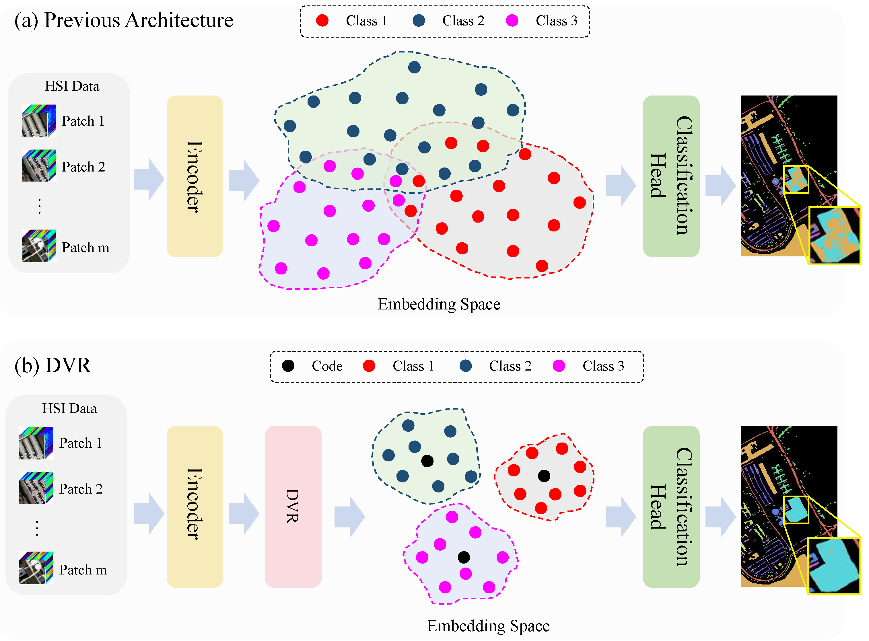
  • We propose a novel discrete vector representation (DVR) strategy. Distinguished from previous approaches of optimizing network structures, DVR offers a fresh perspective on optimizing the distribution of category features to mitigate the misclassification problem. Moreover, it can be effortlessly incorporated into various existing HSI classification methods, thus improving their classification accuracy.
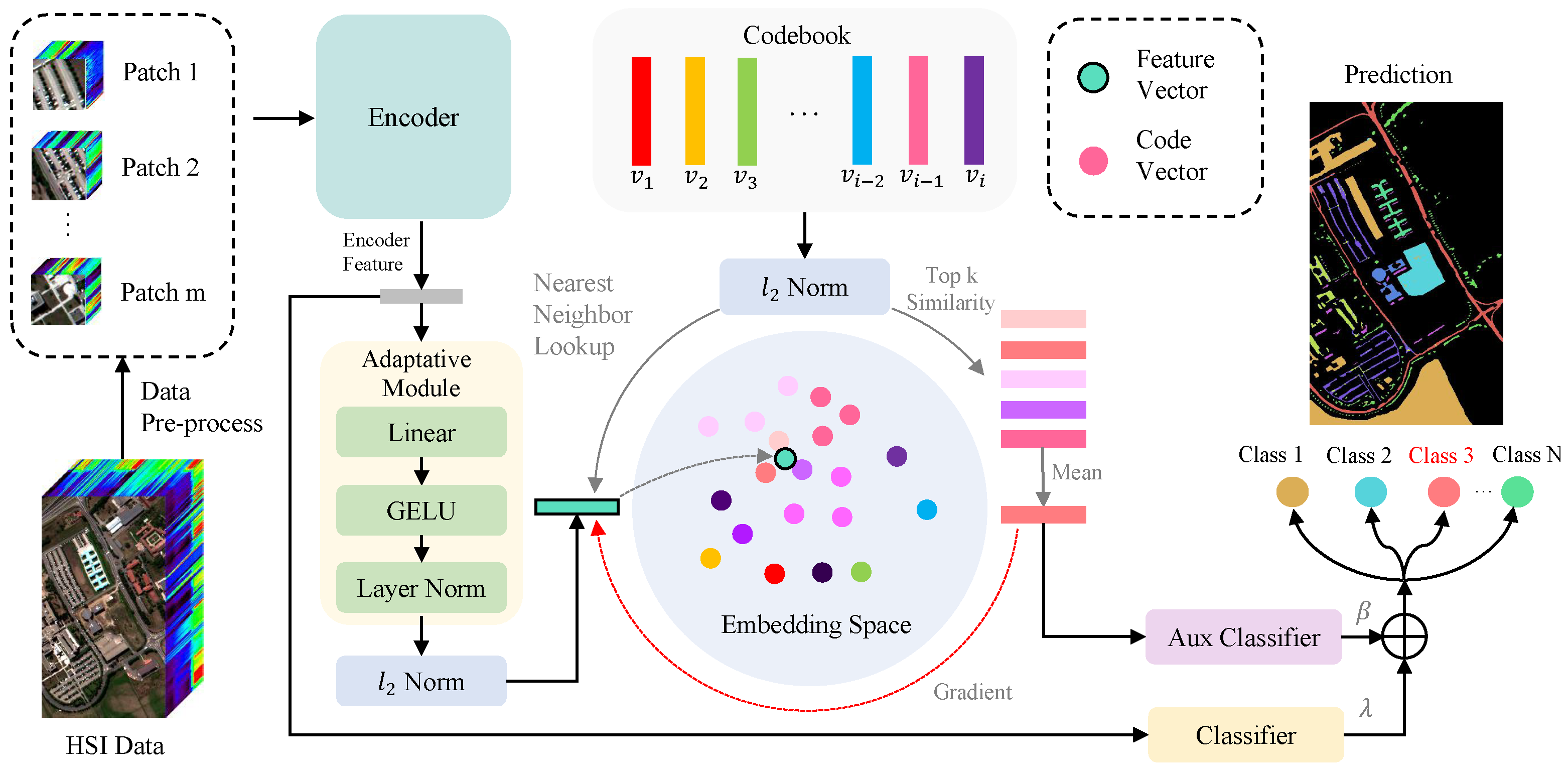
  • We develop the AM, DVCM, and AC to form a complete DVR strategy. The AM aligns the encoded features with the semantic space of the codebook. The DVCM is able to capture essential and stable feature representations in its codebook. The AC enhances classification performance by utilizing representative code information from the codebook. These three components are integrated to improve the discriminability of feature categories and reduce misclassifications.
  • Our comprehensive evaluations demonstrate that the proposed DVR approach with feature distribution optimization can enhance the performance of HSI classifiers. Through extensive experiments and visual analyses conducted on different HSI benchmarks, our DVR approach consistently surpasses other state-of-the-art backbone networks in terms of both classification accuracy and model stability, while requiring merely a minimal increase in parameters.
The remainder of this paper is organized as follows. In Section 2, we review related work on HSI classification methods and schemes for enhancing model performance. Section 3 presents the proposed methodology, which includes the details of our DVR framework and its training process. In Section 4, we describe experimental results of our approach in comparison to baseline methods. Section 5 discusses the limitations of DVR as well as potential directions for future improvements and applications. Finally, Section 6 concludes the article.

2. Related Work

In this section, we overview existing HSI classification approaches, encompassing convolutional neural networks, vision transformers, and schemes for enhancing model performance.

2.1. Convolutional Neural Networks for HSI Classification

With the advancement of deep learning, convolutional neural networks (CNNs) have emerged as powerful tools for HSI classification [13,27,28,29,30,31,32,33,34]. These CNN-based methods have demonstrated impressive achievements by leveraging convolutional layers to extract discriminative features from HSI data. Initially, two-dimensional (2-D) CNNs [27,28] employed convolutional and pooling layers to capture spatial dependencies within HSIs. A pioneering 2-D CNN architecture [27] was proposed for automated high-level feature extraction in HSI classification. Mei et al. [28] concentrated on memory-efficient 2-D CNNs to accelerate the forward step of the network. Then, Song et al. [29] introduced a fusion-based model to aggregate multi-layer features and leverage complementary HSI information. Moreover, Zhao et al. [30] introduced a dual-tunnel CNN to enforce the spatial consistency within deeper network layers. To account for the three-dimensional (3-D) nature of HSIs, many researchers explored 3-D CNNs [13,31,32,33,34] to incorporate spectral and spatial signatures simultaneously. Chen et al. [31] and He et al. [32] proposed an end-to-end multiscale 3-D deep CNN architecture to capture both multiscale spatial and spectral characteristics. To emphasize the importance of spectral–spatial integration, Zhong et al. [33] introduced a spectral–spatial residual network, while Hamida et al. [13] devised a joint spectral–spatial information processing approach. In addition, Mei et al. [34] proposed an unsupervised spatial–spectral feature learning strategy, enabling 3-D convolutional autoencoder networks to extract meaningful features without pixel-wise annotations. Although CNN-based methods show proficiency in extracting distinctive features using 2-D or 3-D structures to enhance feature representation, they generally demand substantial computational resources and fail to capture long-range dependencies of HSI data.

2.2. Vision Transformers for HSI Classification

The limitations have prompted researchers to explore alternative architectures. Recently, ViTs [19] have gained significant attentions for modeling global dependencies in long-range positions and bands of HSI pixels. These transformers [18,20,21,35], equipped with multi-head self-attention mechanisms, show great promise for HSI classification tasks. Hong et al. [18] proposed a backbone network based on the transformer architecture and utilized attention mechanisms to capture subtle spectral differences. Xue et al. [35] introduced a local transformer to incorporate a partial partition restore module for global context dependencies. Sun et al. [20] designed a Spectral–Spatial Feature Tokenization Transformer (SSFTT) to capture spectral–spatial features and high-level semantic features. Additionally, Mei et al. [21] proposed a Group-Aware Hierarchical Transformer (GAHT) for HSI classification, and enhanced the model’s ability to capture local relationships within HSI spectral channels while maintaining a global understanding of spatial–spectral context. Despite the proficiency of ViTs in modeling global dependencies, they usually lack distribution control over the embedding space, thus leading to the cross-aggregation of features.

2.3. Schemes for Enhancing Model Performance

To enhance the model performance, common techniques such as data augmentation and regularization are employed, and vector quantized-variational autoencoder (VQ-VAE) [25] methods leverage discrete representations to enhance the performance. Data augmentation involves transforming or expanding training data to increase the number and diversity of data samples, reducing the model’s reliance on specific data and enhancing its generalization capability. Various techniques, including random rotation, translation, scaling, and noise addition, are employed for data augmentation. Several carefully designed data augmentations were designed by [36,37]. Moreover, regularization techniques constrain the model’s complexity to prevent overfitting to the training data [38,39]. Common regularization methods include adding L1 or L2 norm penalties on loss functions to limit the magnitude of weights. Furthermore, VQ-VAE introduces a codebook learned through a vector-quantized autoencoder model, using an encoder–decoder architecture to transform images into discrete latent codes for enhancing model robustness. Mao et al. [26] demonstrated the use of discrete representations to strengthen model robustness by preserving the overall structure of an image while disregarding minor local details. Hu et al. [40] designed a discrete codebook for encoded feature representation, which helps combats semantic noise with reduced transmission overhead. These researchers demonstrated that discrete representation is an efficient scheme to achieve satisfactory performance. Data augmentation and regularization techniques have been commonly used in existing hyperspectral classification models to enhance model performance from the perspective of data or the model network. However, the current research in HSI classification mainly focuses on the design of new models [41], neglecting the improvement of model performance. Our proposed strategy aims to incorporate discrete representation schemes from the perspective of optimizing the feature space to boost model performance, thereby addressing the existing research gap in techniques.

3. Methods

3.1. Overall Architecture

The architecture overview of the proposed approach is shown in Figure 3. Based on the encoder and classifier, our DVR incorporates the Adaptive Module (AM), DVCM, and auxiliary classifier (AC) into the existing classification model by optimizing the feature distribution to improve its classification performance. Specifically, given the original HSI data { x } R H × W × C (C denotes the spectral bands and H × W is the spatial resolution), we divide it into N patches { x i p } i = 1 N in the preprocessing stage. Firstly, we established a codebook to discretize the embedding space and facilitate the extraction and storage of category representation vectors using our designed DVCM. Subsequently, the encoder processed the inputted patch data to obtain class representation, and the AM fine-tuned the encoded feature to align with the embedding space of the codebook. The top k nearest codes to the encoded feature were chosen and averaged to generate the auxiliary class descriptor. This descriptor was then fed into an AC to assist in the prediction. By leveraging the DVCM and AC during the gradual training process, encoded features of the same class are clustered closely together, while maintaining a clear separation between features of different classes. This distinctive attribute allowed the existing HSI classification model to capture more robust and representative class features, leading to significant performance improvements. The DVR and its training process are elaborated below. Table 1 details the definition of notations used in the proposed DVR.

3.2. Discrete Vector Representation Strategy

Following the structure illustrated in Figure 3, we employed the encoder f ( · ) to transform a patch x i p R P × P × C into a feature vector e R D , where P and D denote the patch size and the dimension of the encoded feature.
Adaptive Module (AM): The AM is composed of a layer normalization step, a Gaussian error Linear Unit (GeLU) activation function and a linear layer. Layer normalization is a widely used normalization technique in deep learning models that standardizes and rescales the outputs of each neuron. This helps in reducing internal covariate shift, improving training stability and convergence speed, and enhancing the generalization capabilities of the model. The GeLU activation function imitates the behavior of stochastic neurons by multiplying the input x with the value from the cumulative distribution function of the standard normal distribution. This simulation enables the network to adjust to various input distributions, thereby improving its robustness. Additionally, the GeLU activation function provides excellent adaptability and flexibility to accommodate the diversity of codes within the codebook, which is defined as
GELU ( x ) = x Φ ( x ) = x · 1 2 [ 1 + erf ( x / 2 ) ]
where Φ ( x ) represents the standard Gaussian cumulative distribution function, and erf ( x ) = 0 x e t 2 d t .
The AM is capable of aligning the extracted features from the encoder with the semantic framework defined by the codebook, as well as adjusting the feature dimensions to match the codebook dimension. The feature vector e is processed through an Adaptive Module to produce h.
Discrete Vector Constraint Module (DVCM): The DVCM introduces a codebook that leverages discrete vector quantification for capturing category representation. After aligning the embedding features with a created codebook, the codebook of the DVCM is able to represent the embedding space in a discrete format and retain representative features of classes as discrete vectors. Specifically, after h has been 2 -normalized, the vector quantizer looks up the top k nearest neighbor codes in the codebook. These selected codes are then averaged to determine the quantized code for the patch feature. Let { v 1 , v 2 , , v K } ( v j R D c ) represent the codes in the codebook, where K and D c denote the number and dimension of discrete vector, respectively. For each patch feature h, its quantized code v ¯ is determined by
{ z 1 , , z k } = Topk min | | 2 ( h ) 2 ( v j ) | | 2 ,
v ¯ = 1 k j { z 1 , , z k } 2 ( v j ) ,
where the 2 normalization is employed for the codebook lookup and { z 1 , , z k } { 1 , 2 , , K } presents the index of top k nearest vectors in the codebook. Furthermore, Topkmin refers to the selection of the k smallest-distance items from a set based on specified criteria. Due to the non-differentiable nature of the quantization process in Equation (2), the gradient is directly copied from the input of the auxiliary classifier to the encoder output, as depicted in Figure 3. Intuitively, the quantizer identifies the nearest code for each encoder output, and the gradient of the codebook embedding indicates the useful direction for optimizing the encoder. To ensure the codebook captures representative features, the codebook embeddings are updated using an exponential moving average (EMA) [25], which offers enhanced stability for training discrete vectors. The typical formula for updating with momentum is expressed by
v j = γ v j + ( 1 γ ) h ,
where γ represents the decay factor, with a value typically close to 1, that determines the weight of the previous code value in the updated calculation. The training objective for updating the codebook vectors is formulated as
min sg 2 ( h ) 2 ( v ¯ ) 2 2 ,
where the symbol sg [ · ] denotes the stop-gradient operator, which is an identity in the forward pass and yielding zero gradients in the backward pass.
Additionally, the utilization of clustering techniques (K-means) divides the feature vector space into several regions, where each region’s centroid is represented by a vector in the codebook. These vectors effectively encapsulate the entire feature space and extract crucial information. The classification process consists of mapping feature vectors to the nearest codebook vector, thereby converting continuous data into discrete codified forms. These discrete representations not only optimize the feature distribution, but also boost the efficiency of the representation, ultimately enhancing the performance of classification algorithms.
Auxiliary Classifier (AC): After generating the codebook, we utilize the discrete vectors to improve the classification procedure. This enhancement entails combining the classification outcomes of codebook features with the features extracted by the encoder models. This collaborative strategy enhances the discriminative capability of the feature set, thus improving classification performance in HSI tasks.
To clearly describe the role of a codebook in assisting with classification, we visualized the meanings of the encodings present in the codebook, as illustrated in Figure 4. The different codes in the codebook represent feature information for different categories, for instance, in the Salinas (SA) dataset, code 21 represents the category “Vinyard_untrained”. By utilizing representative code information from the codebook, samples can be classified more accurately. During the validation phase, we enhanced the primary classification procedure by incorporating outcomes obtained from the codebook features. As illustrated in Figure 5, we selected the top five closest codes within the embedding space and averaged them to generate our auxiliary class descriptor. By merging predictions from both the primary and codebook-based classifications, we harnessed the complementary information within the codebook features to enhance classification performance. This dual classification strategy improved the model’s capacity to accurately classify diverse and intricate data instances. The output o of the classification results following the combination of scores is as follows:
o = λ p + β a ,
where p denotes the output of the primary classifier (PC) using the encoded features, and a represents the output from the AC using the codebook features. We carefully tuned parameters λ and β to balance the contributions of primary and auxiliary classifiers, where λ = 0.75 and β = 0.25 .
Building upon the integration of codebook features with encoder models, our approach introduces a novel loss function tailored to optimize the collaborative utilization of both feature sets. This loss function crucially underpins the dual-classification strategy, and guarantees that each element of the feature representation contributes optimally to the ultimate classification accuracy. Our loss function consists of three components:
L = L C E ( t , p ) + 2 ( h ) sg 2 ( v ¯ ) 2 2 + L C E ( t , a ) ,
where t represent the ground truth. In addition, we adopted the Cross-Entropy (CE) loss function [42] to calculate the classification loss:
L C E ( y c , y ^ c ) = c = 1 C y c log ( y ^ c ) ,
where Equation (8) y c denotes the ground truth, and y ^ c denotes the model’s output probability for the i th patch belonging to the class c. Furthermore, C represents the total number of classes.
We summarize the pseudocode for the DVR inference process in Algorithm 1.
Algorithm 1: Inference of DVR
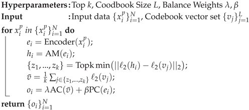
Remotesensing 17 00351 i001

3.3. Train Strategy

We adopted a two-stage training strategy. Initially, we trained the model without the inclusion of codebook features. This initial phase allowed the model to learn basic patterns within the data. After a certain number of epochs, we incorporated the codebook features. The codebook was initialized with a number of samples equivalent to its capacity. These samples were batch-processed through the encoder to extract their features, which were then collectively used to initialize the codebook in the quantizer. This initialization step was crucial as it enhanced the utilization of the codebook, and improved the efficiency of the training process. Furthermore, introducing these features at a later stage enabled us to leverage their discriminative capabilities. This two-stage training strategy ensured that the model first learns simple features and then progressively refines its understanding by incorporating more representative discrete vector features.

4. Experiment Results

In this section, we evaluate the effectiveness of our DVR by employing four standard HSI datasets including Salinas (SA), Pavia University (PU), HyRANK-Loukia (HR-L), and WHU-Hi-HanChuan (HC) [43], which are extensively utilized for classification tasks. Then, we present the implementation details and evaluation metrics. Next, we conduct both qualitative and quantitative analyses compared to the state-of-the-art (SOTA) results. Last, we perform ablation experiments to gauge the impact of different modules and hyper-parameters on classification accuracy.

4.1. Data Description

We allocated varying proportions of labeled samples across different datasets. Specifically, for the SA and PU datasets, we randomly selected 1% of the labeled samples for training, 1% for validation, and 98% for testing. For the HR-L dataset, we designated 3% of the labeled samples for training, 3% for validation, and 94% for testing. As for the HC dataset, we used 0.2% of the samples for training, 0.2% for validation, and 99.6% for testing. The fixed number of training and testing samples can be found in Table 2.

4.1.1. Salinas

The SA dataset was captured through the use of the Airborne Visible/Infrared Imaging Spectrometer (AVIRIS) sensor over the Salinas Valley, California, USA. It is composed of 204 spectral bands after discarding the 20 water absorption bands, covering range from 400 nm to 2500 nm. The image size is 512 × 217 pixels with a ground sampling distance of 3.7 m. It includes 16 different land cover classes. (https://www.ehu.eus/ccwintco/index.php/Hyperspectral_Remote_Sensing_Scenes#Salinas (accessed on 18 January 2025)).

4.1.2. Pavia University

The PU dataset was acquired utilizing the Reflective Optics System Imaging Spectrometer (ROSIS) sensor over the area of Pavia University and its surroundings in Italy. It comprises 103 spectral bands, spanning range from 430 nm to 860 nm. The image size is 610 × 340 pixels with a ground sampling distance of 1.3 m, encompassing nine different land cover categories (https://www.ehu.eus/ccwintco/index.php/Hyperspectral_Remote_Sensing_Scenes#Pavia_University_scene (accessed on 18 January 2025)).

4.1.3. HyRANK-Loukia

The HR-L dataset was sourced by the Hyperion sensor on the Earth Observing-1 satellite. It encompasses a total of 176 spectral bands, spanning range from 400 nm to 2500 nm. The image size is 249 × 945 pixels with a ground sampling distance of 30m within this dataset, and there are 14 distinct land cover classes (https://zenodo.org/records/1222202 (accessed on 18 January 2025)).

4.1.4. WHU-Hi-HanChuan

The HC dataset was collected using the Headwall Nano-Hyperspec sensor mounted on a UAV. It contains 274 spectral bands ranging from 400 nm to 1000 nm, with a spatial resolution of 0.109 m. The imagery size is 1217 × 303 pixels, and the dataset includes seven crop species along with other land cover types such as buildings and water bodies (http://rsidea.whu.edu.cn/resource_WHUHi_sharing.htm (accessed on 18 January 2025)).

4.2. Experiment Setups

4.2.1. Implementation Details

In our experimental setup, we maintained the settings of the encoder models unchanged, while integrating our codebook to assist in the classification process. We implemented our approach using the PyTorch framework and trained it on an NVIDIA GeForce GTX 2080 Ti GPU with 11 GB of memory. The batch size and epoch count were configured at 64 and 300, respectively. To attain the best performance, as reported in [13,18,20,21], both the optimizer and scheduler were maintained at their default configurations. Additionally, data augmentation was employed to mitigate the issue of insufficient training samples in all approaches. For each batch of data in an iteration, one of the five augmentation techniques (vertical flip, horizontal flip, 90° rotation, 180° rotation, and 270° rotation) is randomly chosen with an equal probability.

4.2.2. Evaluation Metrics

To quantitatively evaluate the performance of HSI classification, we employ four metrics: overall accuracy (OA), average accuracy (AA), kappa coefficient ( κ ), and per-class accuracies. OA indicates the percentage of correctly predicted samples out of the total samples. AA represents the mean classification accuracy of each class. The κ coefficient measures the agreement between the ground truth and classification maps. To minimize experimental variability, we randomly split the labeled samples five times, and reported the mean values and standard deviations for these metrics. A lower standard deviation indicates a higher reliability and consistency.

4.2.3. Baseline Models

To demonstrate the effectiveness of the suggested DVR, a number of representative methods are selected for comparative experiments: the 3D-CNN [13], SpectralFormer (SF) [18], SSFTT [20], and GAHT [21]. The 3D-CNN employs a exclusively convolutional architecture, while the SpectralFormer is based on transformer architectures. The SSFTT and GAHT combine convolution and transformer elements in a hybrid architecture. The universality of DVR is better demonstrated through comparative experiments across various architectural types.

4.3. Comparative Experiments

4.3.1. Quantitative Assessment

Table 3, Table 4, Table 5 and Table 6 present the results for the OA, AA, kappa, and each class accuracy using various methods on the Salinas, Pavia University, and HyRANK-Loukia datasets, respectively. The optimal results are highlighted in bold. As the results illustrated, our method outperforms other SOTA methods across all four benchmark datasets. On the SA datasets, our DVR based on respective models achieved significantly higher OA compared with the 3D-CNN and SF, with a difference of 2.39% and 1.22%, respectively. It is obvious that our method also demonstrates lower standard deviations in both OA and specific accuracy for each class. On the PU datasets, our method incorporating DVR with the 3D-CNN achieved the highest improvement of 7.58% in OA. Meanwhile, the kappa value improved from 83.70% ± 1.77% to 94.06% ± 0.46%, indicating a substantial enhancement in model reliability and classification consistency. Similarly, our method based on the SSFTT and GAHT, respectively, showed performance enhancements. On the challenging HR-L dataset, DVR performed much better than the other methods. It is noted that the modified baseline model exhibited greater potential in classifying challenging datasets. This trend highlights the effectiveness of DVR in enhancing the reliability of the classification outcomes under constrained training scenarios.

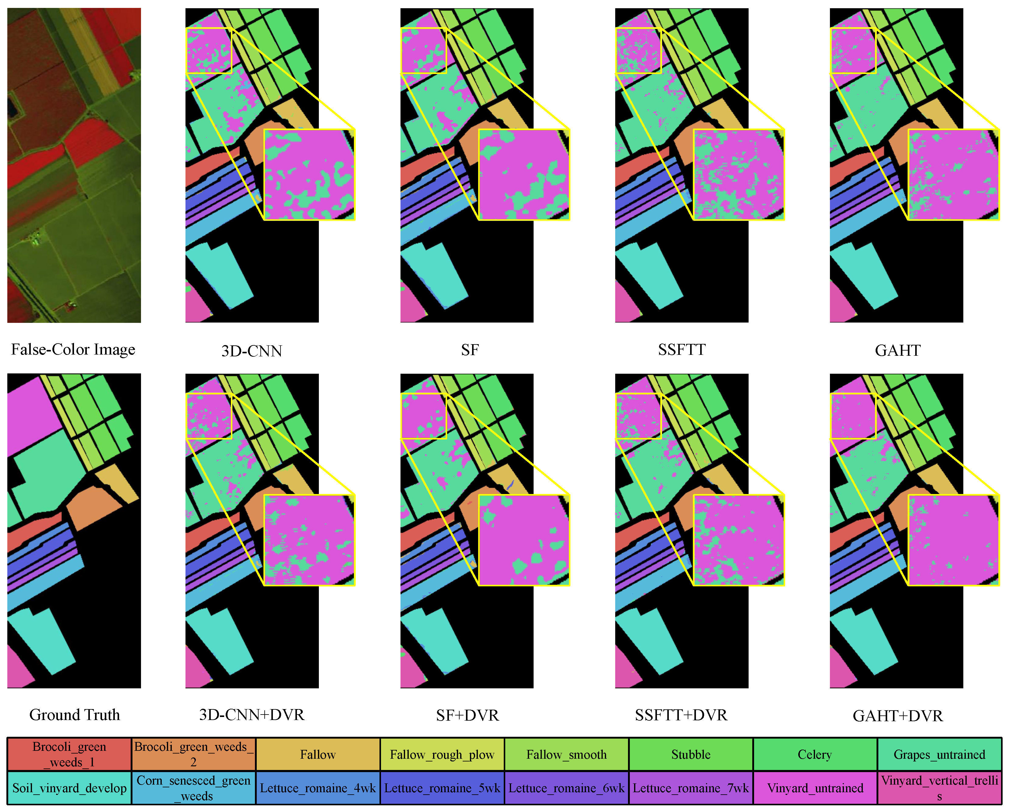
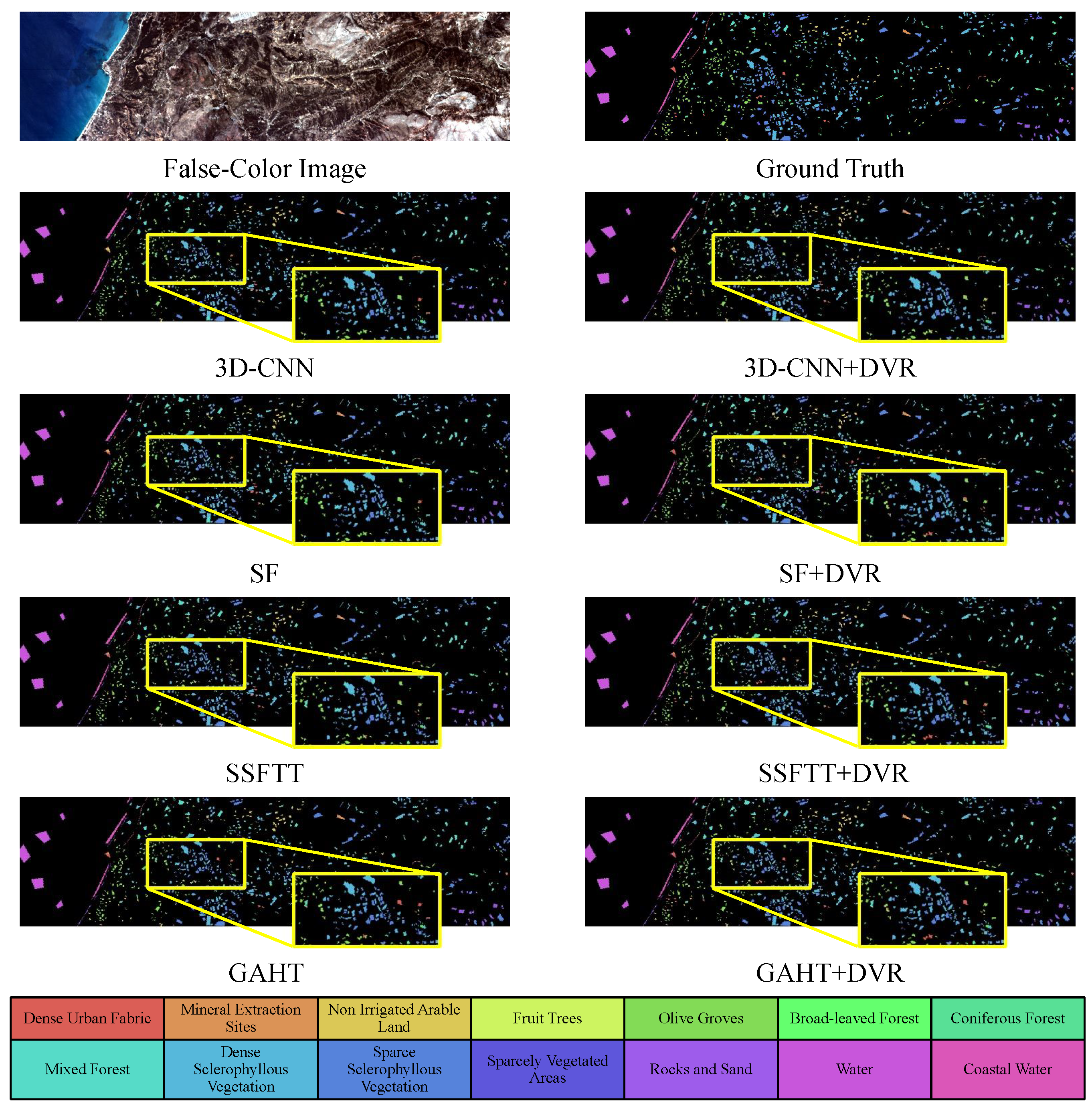
4.3.2. Visual Evaluation

Figure 6, Figure 7, Figure 8 and Figure 9 display the classification maps obtained from various comparison methods on the Salinas, Pavia University, HyRANK-Loukia, and WHU-Hi-HanChuan datasets. We chose the results with the highest OA values from five trials to visualize the predicted samples using different methods for model comparison. Based on the visual comparisons, it is evident that the DVR strategy produces more accurate and less-noise classification maps, which more closely resembles the ground truth.
Furthermore, Figure 10 displays the t-SNE visualization [24] of hidden features from different methods on four distinct datasets. Compared to other methods, DVR demonstrates a more cohesive distribution, with less cross-aggregation and fewer instances of misclassifications among categories.

4.4. Ablation Study

In this subsection, we employ a representative HSI classification approach (SpectralFormer [18]) to conduct extensive ablation experiments, focusing on key components and parameters of DVR that impact classification performance. We investigate the significance of the DVCM and the AC; then, we examine the effects of codebook size, codebook dimension, and the top-k nearest vectors from the codebook. To assess the impact of individual hyper-parameters on classification performance, we employ a systematic grid search [44] approach and alter one hyper-parameter at a time while fixing the values of others. Table 7 provides a summary of the hyper-parameter configurations that yields the highest classification accuracy across the four datasets.

4.4.1. Impact of DVCM

Table 8 displays the results from the ablation study of the DVCM on the PU dataset using the SpectralFormer backbone. The baseline model attains an OA of 88.80% ± 0.94%. By incorporating the AM and AC, our model improves the OA to 89.32% ± 0.85%. Taking into account these results, the inclusion of the DVCM enabled our model to achieve the highest OA of 90.90% ± 0.50%, underscoring the substantial performance enhancement facilitated by the codebook.

4.4.2. Codebook Size

As shown in Table 9, the analysis results demonstrate the impact of codebook size on OA. In the case of the SA dataset, we increased the codebook size from 70 to 100, and the OA was improved from 91.99% to 92.19%. However, when the size further increased to 150, there was a slight decrease in OA to 91.93%. Similarly, for the HR-L dataset, an initial increase in OA from 74.02% to 74.26% was observed when the codebook size was enlarged from 70 to 100. Nevertheless, when the codebook size reached 150, the OA dropped to 73.90%. It is noted that beyond a certain threshold (100), larger codebooks result in inefficiencies or over-parameterization in the model. This suggests that a moderate enlargement in the codebook size can help in capturing more intricate data characteristics and slightly enhance model performance. For the PU dataset, a slight variation appeared in the trend, with the highest OA of 90.90% achieved using a codebook size of 70. As the codebook size increased from 70 to 100 and then to 150, the OA decreased to 90.63% and 90.38%, respectively. This trend highlights that a smaller codebook size (70) is more appropriate for the PU dataset as it aligns with its intrinsic characteristics featuring fewer categories.

4.4.3. Codebook Dimension

We analyze the impact of the codebook dimension on the OA of the SpectralFormer model enhanced by our methodology on the PU dataset. Table 10 clearly demonstrates that varying the codebook dimension leads to subtle differences in model performance. Specifically, the codebook dimension was varied across five different sizes: 32, 64, 128, 256, and 512. The highest OA, at 90.90% ± 0.50%, was achieved with a codebook dimension of 64. This indicates an optimal setting at the size of 64, where the model was capable of effectively capturing essential features without excessive redundancy. As the dimension increased from 64 to 128, there was a slight decrease in OA to 90.59% ± 0.40%. This trend continued with further increments to 256 and 512, resulting in OA dropping slightly to 90.30% ± 0.60% and 90.58% ± 0.60%, respectively. These observations suggest that larger codebook dimensions do not confer better performance, as informative features become diluted within a larger embedding space. The consistent OA across all settings highlights the stability of the DVR model configuration. Our model maintains high performance regardless of substantial changes in the codebook dimension.

4.4.4. Top-k Selection

We investigate the impact of the Top-k parameter on the performance of our model, as detailed in Table 11. Here, Top-k denotes the k codes from the codebook that were closest to the encoder features. These codes were averaged before being fed into the AC. All experiments were carried out on the PU dataset with a consistent configuration where the codebook size was 70 and the codebook dimension was 64. With Top-k = 1, our model achieved an OA of 90.79% ± 0.58%, indicating a highly focused representation based on the most relevant code. Increasing to 5, the OA was slightly improved to 90.90% ± 0.50%, and it suggests that incorporating additional relevant codes can enhance model performance by providing a richer feature representation. However, expanding to 10 led to a slight decrease in OA to 90.75% ± 0.51%, indicating that including too many codes may dilute the feature representation, potentially introducing noise or less relevant information. These results demonstrate that the Top-k parameter has a nuanced impact on model accuracy, highlighting that a moderate number of codes offers a better balance between accuracy and feature representation.

4.4.5. Impact of AC

We evaluate the impact of AC on the OA of our model. We conducted experiments on the PU dataset using the SpectralFormer backbone with and without the AC, as shown in Table 12. The naive SpectralFormer achieved an OA of 88.80% ± 0.94%. When incorporating our modifications into the SpectralFormer without AC, we observed an improvement in OA to 90.66% ± 0.81%. Furthermore, the inclusion of the AC in the modified SpectralFormer led to a further enhancement in OA to 90.90% ± 0.50%. These results clearly demonstrate the positive contribution of the AC to both model accuracy and stability.

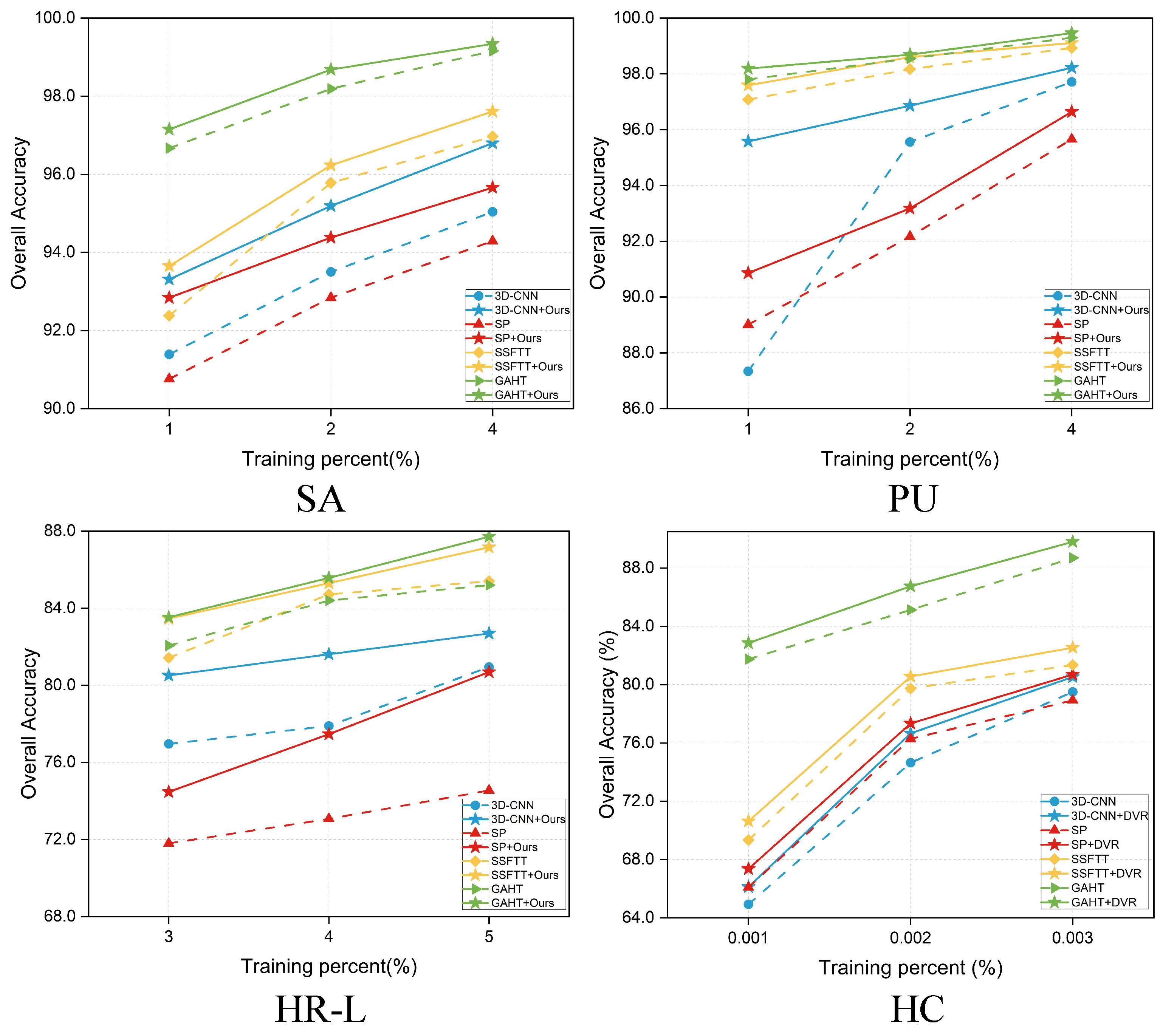
4.5. Robustness Evaluation

Figure 11 displays the results of OA achieved by different methods with different proportions of training samples. To assess the stability and robustness of our proposed method, we randomly selected 1%, 2%, and 4% of labeled samples for the SA and the PU datasets, and 3%, 4%, and 5% for the HR-L dataset. Our method consistently outperformed other methods in all scenarios, which highlights the robustness of our model. The OA of the 3D-CNN was obviously low when training data were limited. However, when our method was integrated, it significantly enhanced the performance of the 3D-CNN. Varying degrees of improvement were also observed in other methods. The most significant enhancement was pronounced in the HR-L dataset. As the volume of training data increased, our method maintained higher accuracy than the other baselines. As the OA approached 100%, the rate of improvement diminished, and the observed marginal effects could be logically explained.

4.6. Computational Cost

This subsection evaluates the incremental computational cost of enhancing the SpectralFormer model with various components within our methodology. We analyzed the impact of integrating the AM, DVCM, and AC on the total number of parameters, trainable parameters, and FLOPs (floating point operations per second). In Table 13, the baseline configuration of SpectralFormer includes 352,405 parameters, all of which are trainable, with a computational workload of 16.235776 million FLOPs. To be specific, with adding AM, the parameters and computational cost experienced a slight increase by 1.18% and 0.025%, respectively. Furthermore, the introduction of the DVCM led to a total parameter increase of 6.31% and a 0.053% rise in FLOPs, while maintaining the trainable parameters constant. This highlights its role as a static feature extractor. Incorporating AC further raised both total and trainable parameters by 6.61% and 1.48%, respectively. The computational costs were minimally increased by 0.059%. It was emphasized that the increases in parameter count and computational load brought about by our proposed DVR were extremely negligible.

5. Discussion

The proposed DVR method, while effective, has certain limitations. The performance shows slight sensitivity to codebook parameters, such as its size and dimension, which may require moderate tuning to achieve optimal results. An oversized codebook may increase computational costs, while an undersized one might fail to capture feature diversity effectively. Future work could focus on optimizing the codebook’s efficiency through advanced encoding algorithms, as well as leveraging automated hyper-parameter tuning methods to reduce the reliance on manual adjustments. Exploring dynamic codebook adjustment could further enhance the scalability and applicability of DVR. In future ocean applications, the visual or spectral differences between classes (e.g., in tasks such as sea ice detection or algal bloom prediction) can be very subtle, making it potentially difficult for existing models to distinguish between them effectively. DVR can leverage the codebook to regulate features, thereby enlarging the distance between features of different classes. This will enable more effective and accurate classification in such challenging scenarios.

6. Conclusions

To mitigate the common misclassification issues in current models for HSI classification, this article introduces an innovative DVR strategy that leverages discrete vectors from the codebook to regulate embedding features. This plug-and-play method enables models to attain a more robust aggregated distribution in the embedding space, thereby enhancing the overall performance of HSI classification. Experimental results conducted on four HSI benchmarks confirm the superiority of our proposed method on both the visual quality of classification maps and quantitative metrics compared to baseline models. Specifically, our DVR improves the OA of the 3D-CNN by 7.58% on the PU dataset and enhances the OA of SpectralFormer by more than 1% across all four datasets. Additionally, integrating DVR into SpectralFormer increases its trainable parameters by only 1.48% and computational cost by just 0.059%. In future work, we will extend the applications of our method to a wider range of models to further enhance performance and explore the potential of our approach in the marine domain, such as sea ice detection and algal bloom prediction.

Author Contributions

Conceptualization, J.L., H.W., X.Z. and J.W.; methodology, J.L., H.W., X.Z. and J.W.; software, H.W., X.Z. and J.W.; validation, J.L. and P.Z.; formal analysis, P.Z.; investigation, J.L. and H.W.; resources, P.Z.; data curation, T.Z.; writing—original draft preparation, J.L., H.W., X.Z. and J.W.; writing—review and editing, H.W., X.Z., T.Z. and P.Z.; visualization, H.W.; supervision, J.L. and P.Z.; project administration, J.L. and P.Z.; funding acquisition, J.L., P.Z. and T.Z. All authors have read and agreed to the published version of the manuscript.

Funding

This work was supported in part by the National Natural Science Foundation of China under Grant 62171252, in part by the Fundamental Research Funds for the Central Universities under Grant 00007764, in part by the Natural Science Foundation of China under Grant 42201386, in part by the Interdisciplinary Research Project for Young Teachers of USTB (Fundamental Research Funds for the Central Universities: FRF-IDRY-22-018), and Fundamental Research Funds for the Central Universities of USTB: FRF-TP-24-060A.

Data Availability Statement

The original contributions presented in the study are included in the article, further inquiries can be directed to the corresponding author.

Conflicts of Interest

The authors declare no conflicts of interest.

References

  1. Bioucas-Dias, J.M.; Plaza, A.; Camps-Valls, G.; Scheunders, P.; Nasrabadi, N.; Chanussot, J. Hyperspectral remote sensing data analysis and future challenges. IEEE Geosci. Remote Sens. Mag. 2013, 1, 6–36. [Google Scholar] [CrossRef]
  2. Hu, C. Hyperspectral reflectance spectra of floating matters derived from Hyperspectral Imager for the Coastal Ocean (HICO) observations. Earth Syst. Sci. Data 2022, 14, 1183–1192. [Google Scholar] [CrossRef]
  3. Grøtte, M.E.; Birkeland, R.; Honoré-Livermore, E.; Bakken, S.; Garrett, J.L.; Prentice, E.F.; Sigernes, F.; Orlandić, M.; Gravdahl, J.T.; Johansen, T.A. Ocean color hyperspectral remote sensing with high resolution and low latency—The HYPSO-1 CubeSat mission. IEEE Trans. Geosci. Remote Sens. 2021, 60, 1–19. [Google Scholar] [CrossRef]
  4. Li, S.; Song, W.; Fang, L.; Chen, Y.; Ghamisi, P.; Benediktsson, J.A. Deep learning for hyperspectral image classification: An overview. IEEE Trans. Geosci. Remote Sens. 2019, 57, 6690–6709. [Google Scholar] [CrossRef]
  5. Kumar, B.; Dikshit, O.; Gupta, A.; Singh, M.K. Feature extraction for hyperspectral image classification: A review. Int. J. Remote Sens. 2020, 41, 6248–6287. [Google Scholar] [CrossRef]
  6. Yang, X.; Cao, W.; Lu, Y.; Zhou, Y. QTN: Quaternion transformer network for hyperspectral image classification. IEEE Trans. Circuits Syst. Video Technol. 2023, 33, 7370–7384. [Google Scholar] [CrossRef]
  7. Fauvel, M.; Benediktsson, J.A.; Chanussot, J.; Sveinsson, J.R. Spectral and spatial classification of hyperspectral data using SVMs and morphological profiles. IEEE Trans. Geosci. Remote Sens. 2008, 46, 3804–3814. [Google Scholar] [CrossRef]
  8. Pal, M.; Foody, G.M. Feature selection for classification of hyperspectral data by SVM. IEEE Trans. Geosci. Remote Sens. 2010, 48, 2297–2307. [Google Scholar] [CrossRef]
  9. Fan, J.; Chen, T.; Lu, S. Superpixel guided deep-sparse-representation learning for hyperspectral image classification. IEEE Trans. Circuits Syst. Video Technol. 2017, 28, 3163–3173. [Google Scholar] [CrossRef]
  10. Li, J.; Zhao, X.; Li, Y.; Du, Q.; Xi, B.; Hu, J. Classification of hyperspectral imagery using a new fully convolutional neural network. IEEE Geosci. Remote Sens. Lett. 2018, 15, 292–296. [Google Scholar] [CrossRef]
  11. Hu, J.F.; Huang, T.Z.; Deng, L.J.; Jiang, T.X.; Vivone, G.; Chanussot, J. Hyperspectral image super-resolution via deep spatiospectral attention convolutional neural networks. IEEE Trans. Neural Netw. Learn. Syst. 2021, 33, 7251–7265. [Google Scholar] [CrossRef] [PubMed]
  12. Pu, C.; Huang, H.; Shi, X.; Wang, T. Semisupervised spatial-spectral feature extraction with attention mechanism for hyperspectral image classification. IEEE Geosci. Remote Sens. Lett. 2022, 19, 1–5. [Google Scholar] [CrossRef]
  13. Hamida, A.B.; Benoit, A.; Lambert, P.; Amar, C.B. 3-D deep learning approach for remote sensing image classification. IEEE Trans. Geosci. Remote Sens. 2018, 56, 4420–4434. [Google Scholar] [CrossRef]
  14. Cao, X.; Xu, L.; Meng, D.; Zhao, Q.; Xu, Z. Integration of 3-dimensional discrete wavelet transform and Markov random field for hyperspectral image classification. Neurocomputing 2017, 226, 90–100. [Google Scholar] [CrossRef]
  15. Cao, X.; Zhou, F.; Xu, L.; Meng, D.; Xu, Z.; Paisley, J. Hyperspectral image classification with Markov random fields and a convolutional neural network. IEEE Trans. Image Process. 2018, 27, 2354–2367. [Google Scholar] [CrossRef] [PubMed]
  16. Xie, J.; He, N.; Fang, L.; Ghamisi, P. Multiscale densely-connected fusion networks for hyperspectral images classification. IEEE Trans. Circuits Syst. Video Technol. 2020, 31, 246–259. [Google Scholar] [CrossRef]
  17. Ran, R.; Deng, L.J.; Zhang, T.J.; Chang, J.; Wu, X.; Tian, Q. KNLConv: Kernel-space non-local convolution for hyperspectral image super-resolution. IEEE Trans. Multimed. 2024, 26, 8836–8848. [Google Scholar] [CrossRef]
  18. Hong, D.; Han, Z.; Yao, J.; Gao, L.; Zhang, B.; Plaza, A.; Chanussot, J. SpectralFormer: Rethinking hyperspectral image classification with transformers. IEEE Trans. Geosci. Remote Sens. 2021, 60, 1–15. [Google Scholar] [CrossRef]
  19. Dosovitskiy, A.; Beyer, L.; Kolesnikov, A.; Weissenborn, D.; Zhai, X.; Unterthiner, T.; Dehghani, M.; Minderer, M.; Heigold, G.; Gelly, S.; et al. An image is worth 16x16 words: Transformers for image recognition at scale. arXiv 2020, arXiv:2010.11929. [Google Scholar]
  20. Sun, L.; Zhao, G.; Zheng, Y.; Wu, Z. Spectral–spatial feature tokenization transformer for hyperspectral image classification. IEEE Trans. Geosci. Remote Sens. 2022, 60, 5522214. [Google Scholar] [CrossRef]
  21. Mei, S.; Song, C.; Ma, M.; Xu, F. Hyperspectral image classification using group-aware hierarchical transformer. IEEE Trans. Geosci. Remote Sens. 2022, 60, 5539014. [Google Scholar] [CrossRef]
  22. Song, L.; Feng, Z.; Yang, S.; Zhang, X.; Jiao, L. Interactive Spectral-Spatial Transformer for Hyperspectral Image Classification. IEEE Trans. Circuits Syst. Video Technol. 2024, 34, 8589–8601. [Google Scholar] [CrossRef]
  23. Hong, D.; Gao, L.; Hang, R.; Zhang, B.; Chanussot, J. Deep encoder–decoder networks for classification of hyperspectral and LiDAR data. IEEE Geosci. Remote Sens. Lett. 2020, 19, 1–5. [Google Scholar] [CrossRef]
  24. Van der Maaten, L.; Hinton, G. Visualizing data using t-SNE. J. Mach. Learn. Res. 2008, 9, 2579–2605. [Google Scholar]
  25. Van Den Oord, A.; Vinyals, O.; Kavukcuoglu, K. Neural discrete representation learning. In Proceedings of the Advances in Neural Information Processing Systems, Long Beach, CA, USA, 4–9 December 2017; Volume 30, pp. 6309–6318. [Google Scholar]
  26. Mao, C.; Jiang, L.; Dehghani, M.; Vondrick, C.; Sukthankar, R.; Essa, I. Discrete Representations Strengthen Vision Transformer Robustness. In Proceedings of the International Conference on Learning Representations (ICLR), Online, 25–29 April 2022. [Google Scholar]
  27. Makantasis, K.; Karantzalos, K.; Doulamis, A.; Doulamis, N. Deep supervised learning for hyperspectral data classification through convolutional neural networks. In Proceedings of the IEEE International Geoscience and Remote Sensing Symposium (IGARSS), Milan, Italy, 26–31 July 2015; pp. 4959–4962. [Google Scholar]
  28. Mei, S.; Chen, X.; Zhang, Y.; Li, J.; Plaza, A. Accelerating convolutional neural network-based hyperspectral image classification by step activation quantization. IEEE Trans. Geosci. Remote Sens. 2021, 60, 1–12. [Google Scholar]
  29. Song, W.; Li, S.; Fang, L.; Lu, T. Hyperspectral image classification with deep feature fusion network. IEEE Trans. Geosci. Remote Sens. 2018, 56, 3173–3184. [Google Scholar] [CrossRef]
  30. Zhao, X.; Tao, R.; Li, W.; Li, H.C.; Du, Q.; Liao, W.; Philips, W. Joint classification of hyperspectral and LiDAR data using hierarchical random walk and deep CNN architecture. IEEE Trans. Geosci. Remote Sens. 2020, 58, 7355–7370. [Google Scholar] [CrossRef]
  31. Chen, Y.; Jiang, H.; Li, C.; Jia, X.; Ghamisi, P. Deep feature extraction and classification of hyperspectral images based on convolutional neural networks. IEEE Trans. Geosci. Remote Sens. 2016, 54, 6232–6251. [Google Scholar] [CrossRef]
  32. He, M.; Li, B.; Chen, H. Multi-scale 3D deep convolutional neural network for hyperspectral image classification. In Proceedings of the IEEE International Conference on Image Processing (ICIP), Beijing, China, 17–20 September 2017; pp. 3904–3908. [Google Scholar]
  33. Zhong, Z.; Li, J.; Luo, Z.; Chapman, M. Spectral–spatial residual network for hyperspectral image classification: A 3-D deep learning framework. IEEE Trans. Geosci. Remote Sens. 2017, 56, 847–858. [Google Scholar] [CrossRef]
  34. Mei, S.; Ji, J.; Geng, Y.; Zhang, Z.; Li, X.; Du, Q. Unsupervised spatial–spectral feature learning by 3D convolutional autoencoder for hyperspectral classification. IEEE Trans. Geosci. Remote Sens. 2019, 57, 6808–6820. [Google Scholar] [CrossRef]
  35. Xue, Z.; Xu, Q.; Zhang, M. Local transformer with spatial partition restore for hyperspectral image classification. IEEE J. Sel. Top. Appl. Earth Obs. Remote Sens. 2022, 15, 4307–4325. [Google Scholar] [CrossRef]
  36. Hendrycks, D.; Basart, S.; Mu, N.; Kadavath, S.; Wang, F.; Dorundo, E.; Desai, R.; Zhu, T.; Parajuli, S.; Guo, M.; et al. The many faces of robustness: A critical analysis of out-of-distribution generalization. In Proceedings of the IEEE/CVF International Conference on Computer Vision (ICCV), Montreal, BC, Canada, 11–17 October 2021; pp. 8340–8349. [Google Scholar]
  37. Steiner, A.; Kolesnikov, A.; Zhai, X.; Wightman, R.; Uszkoreit, J.; Beyer, L. How to train your vit? data, augmentation, and regularization in vision transformers. arXiv 2021, arXiv:2106.10270. [Google Scholar]
  38. Wang, H.; Ge, S.; Lipton, Z.; Xing, E.P. Learning robust global representations by penalizing local predictive power. In Proceedings of the Advances in Neural Information Processing Systems, Vancouver, BC, Canada, 8–14 December 2019; Volume 32, pp. 10506–10518. [Google Scholar]
  39. Huang, Z.; Wang, H.; Xing, E.P.; Huang, D. Self-challenging improves cross-domain generalization. In Proceedings of the European Conference on Computer Vision (ECCV), Glasgow, UK, 23–28 August 2020; pp. 124–140. [Google Scholar]
  40. Hu, Q.; Zhang, G.; Qin, Z.; Cai, Y.; Yu, G.; Li, G.Y. Robust semantic communications with masked VQ-VAE enabled codebook. IEEE Trans. Wirel. Commun. 2023, 22, 8707–8722. [Google Scholar] [CrossRef]
  41. Xi, B.; Li, J.; Diao, Y.; Li, Y.; Li, Z.; Huang, Y.; Chanussot, J. Dgssc: A deep generative spectral-spatial classifier for imbalanced hyperspectral imagery. IEEE Trans. Circuits Syst. Video Technol. 2022, 33, 1535–1548. [Google Scholar] [CrossRef]
  42. Mao, A.; Mohri, M.; Zhong, Y. Cross-entropy loss functions: Theoretical analysis and applications. In Proceedings of the International Conference on Machine Learning (ICML), Honolulu, HI, USA, 23–29 July 2023; pp. 23803–23828. [Google Scholar]
  43. Zhong, Y.; Hu, X.; Luo, C.; Wang, X.; Zhao, J.; Zhang, L. WHU-Hi: UAV-borne hyperspectral with high spatial resolution (H2) benchmark datasets and classifier for precise crop identification based on deep convolutional neural network with CRF. Remote Sens. Environ. 2020, 250, 112012. [Google Scholar] [CrossRef]
  44. Brito, J.A.; McNeill, F.E.; Webber, C.E.; Chettle, D.R. Grid search: An innovative method for the estimation of the rates of lead exchange between body compartments. J. Environ. Monit. 2005, 7, 241–247. [Google Scholar] [CrossRef] [PubMed]
Figure 1. Misclassification due to encoded features overlap. (a) Category results of prediction. (b) Category results of label. The t-SNE visualization of encoded features from SpectralFormer [18] on the Pavia University dataset clearly demonstrates that SpectralFormer incorrectly categorizes instances (labeled as blue) as belonging to the yellow category, while also misclassifying instances (labeled as blue and pink) as belonging to the red category. The overlap of encoded features significantly contributes to classification inaccuracies.
Remotesensing 17 00351 g001
Figure 2. Comparison between previous architecture and our DVR strategy. (a) Previous architecture. Previous architecture typically comprises an encoder and a classification head, however, it faces difficulties due to the disorderly distribution of encoded features, resulting in a decline in classification accuracy. (b) DVR. Our DVR approach integrates the discrete vector representation into the embedding space of encoded feature, aiming to optimize the distribution of encoded features by making features of the same category more compactly clustered and reduce the likelihood of misclassification by the classifier.
Remotesensing 17 00351 g002
Figure 3. The proposed DVR framework for HSI classification. Firstly, the encoder in the model extracts spatial–spectral features from each patch, and these features are then adjusted by the Adaptive Module to align with the embedding space defined by the codebook. This codebook comprises multiple discrete vectors that represent different classes, which are refined through the DVCM (between AM and AC) during training iterations. Subsequently, the framework calculates the auxiliary (Aux) class descriptor by averaging the top k nearest vectors from the codebook. The descriptor is employed by the Aux classifier to predict the class of each input patch. Ultimately, this prediction combines with the output of primary classifier to generate a classified image as final output.
Remotesensing 17 00351 g003
Figure 4. Codebook visualization. The different codes in the codebook represent the feature information for various categories. For instance, in the SA dataset, code 21 corresponds to the category “Vinyard untrained”.
Remotesensing 17 00351 g004
Figure 5. Dual classification strategy. We select the top five closest codes within the embedding space and average them to generate our auxiliary class descriptor. By merging predictions from both the primary and codebook-based classifications, we leverage the complementary information within the codebook features to improve classification performance.
Remotesensing 17 00351 g005
Figure 6. Classification maps by different methods (3D-CNN [13], SF [18], SSFTT [20], GAHT [21]) on the SA dataset with 1% training samples.
Remotesensing 17 00351 g006
Figure 7. Classification maps by different methods (3D-CNN [13], SF [18], SSFTT [20], GAHT [21]) on the PU dataset with 1% training samples.
Remotesensing 17 00351 g007
Figure 8. Classification maps by different methods (3D-CNN [13], SF [18], SSFTT [20], GAHT [21]) on the HR-L dataset with 3% training samples.
Remotesensing 17 00351 g008
Figure 9. Classification maps by different methods (3D-CNN [13], SF [18], SSFTT [20], GAHT [21]) on the HC dataset with 0.2% training samples.
Remotesensing 17 00351 g009
Figure 10. The t-SNE visualization results of encoded features by different methods (3D-CNN [13], SF [18], SSFTT [20], GAHT [21]) on the four datasets. Compared to other methods, DVR demonstrates a more cohesive distribution, with less cross-aggregation and fewer instances of misclassifications among categories.
Remotesensing 17 00351 g010
Figure 11. OA of different models (3D-CNN [13], SF [18], SSFTT [20], GAHT [21]) with different percentages of training samples.
Remotesensing 17 00351 g011
Table 1. Definition of notations used in DVR.
ParametersDefinition
xAn original HSI data
x i p An HSI data patch
f ( · ) Encoder
eThe feature vector from encoder
Φ ( x ) The standard Gaussian cumulative distribution function
hThe feature vector from the Adaptive Module
vThe code in the codebook
zThe index of top k nearest vectors in the codebook
Topkmin The k minest-distance items
γ The decay factor
sg[·]The stop-gradient operator
oThe final output combining two classifiers
aThe output of the auxiliary classifier
pThe output of the primary classifier
tThe ground truth
λ The weight of primary classifier
β The weight of auxiliary classifier
Table 2. The numbers of training, validation, and testing samples in the SA dataset, the PU dataset, the HR-L dataset, and the HC Dataset.
SA (1% for Training)PU (1% for Training)
NO.Class NameTrainVal.TestNO.Class NameTrainVal.Test
1Broccoli_green_weeds_1404019291Asphalt1321336366
2Broccoli_green_weeds_2747535772Meadows37337317,903
3Fallow403918973Gravel42422015
4Fallow_rough_plow282813384Trees62612940
5Fallow_smooth535425715Metal Sheets27271291
6Stubble797938016Bare Soil1001014828
7Celery717234367Bitumen27261277
8Grapes_untrained22522610,8208Bricks73743535
9Soil_vinyard_develop12412459559Shadows1919909
10Corn_sensced_green_weeds65663147-----
11Lettuce_romaine_4wk22211025-----
12Lettuce_romaine_5wk39381850-----
13Lettuce_romaine_6wk1918879-----
14Lettuce_romaine_7wk22211027-----
15Vinyard_untrained1451466977-----
16Vinyard_vertical_trellis36361735-----
Total-1082108351,964--85585641,065
HR-L (3% for Training)HC (0.2% for Training)
NO.Class NameTrainVal.TestNO.Class NameTrainVal.Test
1Dense Urban Fabric892711Strawberry899044,556
2Mineral Extraction Sites22632Cowpea464522,662
3Non Irrigated Arable Land17165093Soybean212010,246
4Fruit Trees32744Sorghum10115332
5Olive Groves424213175Water spinach231195
6Broad-leaved Forest672106Watermelon994515
7Coniferous Forest15154707Greens12125879
8Mixed Forest323210088Trees363617,906
9Dense Sclerophyllous Vegetation11411435659Grass19199431
10Sparse Sclerophyllous Vegetation8484263510Red roof212110,474
11Sparcely Vegetated Areas121238011Gray roof343416,843
12Rocks and Sand141545812Plastic873664
13Water4242130913Bare soil18189080
14Coastal Water141342414Road373718,486
-----15Bright object221132
-----16Water15115175,099
Total-40540512,693--515515256,500
Note: The colors of each category in the table correspond to the colors used in the visualization.
Table 3. Classification performance of various methods on the SA dataset using only 1% training samples.
Method3D-CNN [13]3D-CNN + DVRSF [18]SF + DVRSSFTT [20]SSFTT + DVRGAHT [21]GAHT + DVR
Class
196.48 ± 1.1298.75 ± 1.0495.80 ± 0.8396.91 ± 0.1899.87 ± 0.2699.47 ± 0.85100.00 ± 0.0099.93 ± 0.14
299.92 ± 0.0399.78 ± 0.3699.06 ± 0.4599.03 ± 0.4499.67 ± 0.2799.85 ± 0.1299.99 ± 0.01100.00 ± 0.00
391.47 ± 2.2896.29 ± 0.5294.42 ± 2.8191.85 ± 3.3896.02 ± 3.7497.44 ± 1.9199.40 ± 0.2899.03 ± 1.24
498.07 ± 0.3998.73 ± 0.6993.44 ± 1.7095.80 ± 1.5299.39 ± 0.4199.08 ± 0.6998.55 ± 1.6698.70 ± 1.49
595.60 ± 2.3495.50 ± 2.7392.31 ± 3.0490.18 ± 2.6097.07 ± 2.5198.28 ± 1.2399.06 ± 0.6199.28 ± 0.63
699.34 ± 0.4599.82 ± 0.1899.51 ± 0.5799.45 ± 0.5499.42 ± 0.9799.86 ± 0.1799.99 ± 0.02100.00 ± 0.00
799.45 ± 0.2799.80 ± 0.1798.87 ± 0.4698.64 ± 0.6799.09 ± 0.5899.56 ± 0.4299.89 ± 0.1999.99 ± 0.01
884.13 ± 2.0487.86 ± 2.4285.58 ± 2.3285.88 ± 1.8189.52 ± 2.3988.18 ± 3.0593.66 ± 1.2993.64 ± 1.15
997.33 ± 1.4698.79 ± 1.0696.99 ± 0.9199.12 ± 0.8199.15 ± 0.6199.27 ± 0.5599.96 ± 0.0699.96 ± 0.06
1090.59 ± 1.6893.01 ± 2.1088.20 ± 2.4389.60 ± 1.3292.76 ± 2.1994.70 ± 0.8196.71 ± 2.2597.98 ± 2.03
1181.57 ± 9.0394.71 ± 3.3789.02 ± 1.1191.90 ± 2.5198.15 ± 1.0996.91 ± 2.0398.76 ± 0.7399.31 ± 0.38
1299.34 ± 0.3898.49 ± 1.3298.76 ± 0.6598.91 ± 0.6799.90 ± 0.1099.79 ± 0.2399.83 ± 0.2099.74 ± 0.21
1397.77 ± 2.5094.08 ± 6.8993.54 ± 7.0596.39 ± 5.4096.44 ± 4.0498.44 ± 1.5097.84 ± 2.2298.57 ± 2.04
1496.19 ± 3.1497.06 ± 1.7895.54 ± 2.0296.97 ± 1.3895.94 ± 2.5195.27 ± 2.7097.98 ± 1.7198.02 ± 1.07
1575.29 ± 3.6680.50 ± 3.4776.63 ± 4.9482.88 ± 2.7678.62 ± 4.2784.85 ± 3.0489.69 ± 1.3291.76 ± 2.61
1690.83 ± 4.5993.38 ± 5.3293.50 ± 4.5592.64 ± 2.7196.75 ± 1.5595.45 ± 3.4697.72 ± 2.0498.61 ± 0.35
OA (%)90.89 ± 0.5593.28 ± 0.3291.04 ± 0.6392.26 ± 0.1193.69 ± 0.3494.49 ± 0.3396.80 ± 0.4197.20 ± 0.21
AA (%)93.33 ± 0.6795.41 ± 0.4493.20 ± 0.6194.13 ± 0.2996.11 ± 0.4296.65 ± 0.2298.07 ± 0.1898.41 ± 0.36
κ × 10089.86 ± 0.6192.51 ± 0.3590.03 ± 0.7191.39 ± 0.1292.97 ± 0.3993.86 ± 0.3796.43 ± 0.4596.88 ± 0.24
Train time(s)173.65 ± 0.44184.17 ± 1.37192.51 ± 1.08221.42 ± 1.05171.98 ± 3.26193.48 ± 1.71222.26 ± 1.33243.29 ± 1.31
Test time(s)6.98 ± 0.218.52 ± 0.0519.29 ± 0.0522.43 ± 0.196.91 ± 0.128.68 ± 0.1210.12 ± 0.4511.61 ± 0.38
Table 4. Classification performance of various methods on the PU dataset using only 1% training samples.
Method3D-CNN [13]3D-CNN + DVRSF [18]SF + DVRSSFTT [20]SSFTT + DVRGAHT [21]GAHT + DVR
Class
193.48 ± 1.0795.38 ± 1.6887.87 ± 1.7990.81 ± 0.9495.84 ± 0.9497.20 ± 0.9097.67 ± 1.1697.43 ± 0.69
297.35 ± 1.7199.12 ± 0.3696.29 ± 1.9498.07 ± 0.3999.25 ± 0.7799.39 ± 0.3199.69 ± 0.0999.67 ± 0.18
347.78 ± 7.3281.17 ± 3.2068.40 ± 8.1367.77 ± 5.6489.23 ± 3.2789.48 ± 3.0390.23 ± 4.0190.00 ± 2.58
494.45 ± 1.3696.42 ± 1.2089.70 ± 3.2790.90 ± 2.0097.86 ± 0.7997.81 ± 0.6097.19 ± 0.8797.83 ± 0.33
599.74 ± 0.2399.89 ± 0.15100.00 ± 0.0099.97 ± 0.0499.98 ± 0.0399.94 ± 0.09100.00 ± 0.00100.00 ± 0.00
656.84 ± 4.5392.62 ± 2.1979.94 ± 6.9283.43 ± 1.4298.50 ± 0.7799.23 ± 0.2398.25 ± 1.2599.48 ± 0.40
766.66 ± 8.1882.10 ± 5.9058.25 ± 6.6555.36 ± 5.3692.66 ± 3.8391.34 ± 3.5292.82 ± 5.6698.27 ± 0.78
890.91 ± 1.2991.32 ± 1.8380.69 ± 1.1887.27 ± 1.2590.08 ± 4.5895.33 ± 1.6594.15 ± 1.9495.39 ± 1.09
999.01 ± 0.7599.38 ± 0.3695.82 ± 1.4092.18 ± 0.4699.81 ± 0.1399.61 ± 0.3399.68 ± 0.1099.63 ± 0.27
OA (%)87.95 ± 1.3195.53 ± 0.3588.80 ± 0.9490.90 ± 0.5097.08 ± 0.6497.85 ± 0.2297.89 ± 0.3098.29 ± 0.12
AA (%)82.91 ± 1.9393.04 ± 0.4984.11 ± 1.8685.09 ± 0.9395.91 ± 0.9096.59 ± 0.5296.63 ± 0.5997.52 ± 0.07
κ × 10083.70 ± 1.7794.06 ± 0.4685.09 ± 1.2687.84 ± 0.6696.14 ± 0.897.16 ± 0.2997.19 ± 0.4197.74 ± 0.16
Train time(s)161.01 ± 1.09179.40 ± 2.79221.72 ± 11.13237.73 ± 0.66171.68 ± 0.34187.51 ± 1.27207.99 ± 0.99220.48 ± 1.52
Test time(s)9.05 ± 0.4511.92 ± 0.0929.38 ± 7.2333.62 ± 0.289.15 ± 0.3712.48 ± 0.5017.63 ± 0.4218.79 ± 0.19
Table 5. Classification performance of various methods on the HR-L dataset using only 3% training samples.
Method3D-CNN [13]3D-CNN + DVRSF [18]SF + DVRSSFTT [20]SSFTT + DVRGAHT [21]GAHT + DVR
Class
140.07 ± 3.9447.08 ± 7.2346.49 ± 10.0840.37 ± 7.0864.28 ± 6.0153.58 ± 6.2064.06 ± 10.2771.14 ± 5.08
287.62 ± 8.6083.81 ± 16.6996.83 ± 4.9296.83 ± 6.3586.35 ± 8.6179.37 ± 6.0290.48 ± 10.4390.79 ± 5.35
376.54 ± 6.7881.69 ± 5.5564.95 ± 6.1065.78 ± 5.9980.51 ± 7.0584.83 ± 1.9384.09 ± 5.9185.78 ± 2.23
43.78 ± 4.6344.05 ± 9.652.97 ± 3.865.95 ± 4.4138.11 ± 14.2942.70 ± 14.3235.41 ± 13.6333.24 ± 4.32
577.86 ± 2.6784.87 ± 2.3671.28 ± 5.7077.01 ± 2.7487.64 ± 2.8791.94 ± 0.6689.61 ± 4.2589.96 ± 3.10
640.29 ± 5.8262.29 ± 7.7924.48 ± 10.4018.29 ± 9.4055.05 ± 9.1353.62 ± 4.8242.48 ± 12.5349.24 ± 4.91
748.21 ± 8.2360.89 ± 5.5341.62 ± 4.3847.62 ± 2.4765.53 ± 5.4066.21 ± 5.0461.66 ± 5.2560.81 ± 6.70
861.53 ± 9.1374.13 ± 2.7063.81 ± 5.0463.19 ± 3.1770.42 ± 5.2871.17 ± 7.4671.31 ± 7.9068.69 ± 6.24
982.19 ± 2.5378.59 ± 1.3568.59 ± 2.1974.42 ± 3.3481.91 ± 3.2885.80 ± 2.2783.94 ± 2.1083.36 ± 2.42
1076.70 ± 2.5481.18 ± 0.8671.51 ± 2.5875.29 ± 2.3481.65 ± 2.5782.09 ± 1.2276.51 ± 3.3182.05 ± 2.45
1143.42 ± 15.1661.63 ± 4.5453.63 ± 11.6257.58 ± 5.4165.00 ± 10.9371.00 ± 4.4072.84 ± 5.6572.42 ± 4.49
1291.75 ± 1.5792.45 ± 1.1990.04 ± 6.5290.57 ± 3.4893.97 ± 1.0392.49 ± 1.0192.93 ± 3.2592.88 ± 2.85
13100.00 ± 0.00100.00 ± 0.00100.00 ± 0.00100.00 ± 0.00100.00 ± 0.00100.00 ± 0.00100.00 ± 0.00100.00 ± 0.00
14100.00 ± 0.0099.86 ± 0.19100.00 ± 0.0099.72 ± 0.57100.00 ± 0.0099.95 ± 0.0999.81 ± 0.2399.67 ± 0.35
OA (%)77.07 ± 0.6380.69 ± 0.4171.12 ± 0.4774.26 ± 0.2482.22 ± 0.7683.97 ± 0.1981.98 ± 0.6283.07 ± 0.59
AA (%)66.43 ± 0.7475.18 ± 1.3964.01 ± 1.2565.19 ± 0.8176.46 ± 1.3076.77 ± 1.0976.08 ± 2.2077.15 ± 0.58
κ × 10072.46 ± 0.7277.08 ± 0.4665.66 ± 0.5269.27 ± 0.2278.82 ± 0.8680.87 ± 0.2278.51 ± 0.7079.79 ± 0.67
Train time165.27 ± 7.74175.99 ± 2.25257.05 ± 1.01261.42 ± 3.28185.41 ± 0.34195.18 ± 1.05219.04 ± 0.97230.73 ± 2.03
Test time10.94 ± 1.4112.13 ± 0.1353.05 ± 0.5458.35 ± 1.6313.73 ± 0.3015.45 ± 0.2721.95 ± 0.5622.50 ± 0.14
Table 6. Classification performance of various methods on the HC dataset using only 0.2% training samples.
Method3D-CNN [13]3D-CNN + DVRSF [18]SF + DVRSSFTT [20]SSFTT + DVRGAHT [21]GAHT + DVR
Class
192.14 ± 3.0790.99 ± 2.7790.57 ± 1.5493.39 ± 2.1594.27 ± 1.5492.41 ± 3.9896.35 ± 0.4995.42 ± 0.97
279.04 ± 1.4778.48 ± 1.9770.53 ± 3.3566.02 ± 9.3380.10 ± 4.2181.49 ± 2.4486.13 ± 1.7384.97 ± 3.84
358.81 ± 6.8759.98 ± 4.9061.89 ± 9.7065.80 ± 8.6158.05 ± 6.8256.30 ± 10.7079.62 ± 4.4180.00 ± 6.30
467.01 ± 9.8477.48 ± 3.0849.48 ± 13.6859.50 ± 12.2170.55 ± 11.8378.56 ± 6.2290.32 ± 5.8592.34 ± 2.13
55.56 ± 7.868.82 ± 7.088.02 ± 4.9418.56 ± 10.9413.84 ± 5.707.25 ± 6.247.50 ± 13.4728.44 ± 12.78
61.79 ± 2.259.52 ± 7.557.15 ± 4.435.44 ± 3.2414.05 ± 4.993.39 ± 3.8810.17 ± 6.5826.82 ± 5.03
784.74 ± 8.0880.73 ± 6.0447.31 ± 12.2550.02 ± 11.5664.48 ± 20.8375.23 ± 16.3573.70 ± 5.0378.28 ± 7.55
866.40 ± 2.7261.88 ± 2.1065.11 ± 2.0565.76 ± 2.3869.33 ± 8.3976.31 ± 3.9473.61 ± 4.7173.93 ± 4.08
923.92 ± 6.1332.48 ± 4.9421.18 ± 5.4729.11 ± 8.4648.11 ± 17.5927.40 ± 13.1849.87 ± 7.4366.21 ± 5.78
1037.82 ± 10.6054.09 ± 7.4277.56 ± 3.6868.90 ± 2.8587.80 ± 8.6786.33 ± 4.6692.33 ± 4.0892.09 ± 3.77
1152.83 ± 15.6462.28 ± 7.3171.08 ± 3.5279.54 ± 4.9170.01 ± 14.1683.43 ± 7.0584.58 ± 5.0887.59 ± 8.24
121.92 ± 3.510.04 ± 0.0719.11 ± 10.2621.27 ± 13.2115.13 ± 12.4515.03 ± 7.9612.91 ± 11.9530.84 ± 11.22
1326.81 ± 10.6132.51 ± 8.3636.12 ± 7.8744.36 ± 2.8036.60 ± 13.8540.51 ± 16.0450.91 ± 4.6560.85 ± 5.75
1475.46 ± 4.0379.92 ± 2.6582.53 ± 5.4779.30 ± 6.1974.67 ± 6.0982.70 ± 4.6990.03 ± 2.5488.15 ± 4.97
1533.50 ± 19.3730.09 ± 22.2824.98 ± 12.5022.33 ± 12.0247.60 ± 22.8239.89 ± 15.420.30 ± 0.6017.70 ± 21.52
1698.43 ± 1.2599.04 ± 0.6798.37 ± 0.5098.06 ± 0.7898.43 ± 1.0597.30 ± 2.5099.23 ± 0.4899.12 ± 0.87
OA (%)74.64 ± 1.4476.66 ± 0.5276.28 ± 0.5177.34 ± 0.4579.74 ± 1.6580.56 ± 1.5985.13 ± 0.6286.75 ± 0.77
AA (%)50.39 ± 2.9853.65 ± 1.0951.94 ± 1.5554.21 ± 1.0658.94 ± 2.4258.97 ± 1.8962.35 ± 1.6868.92 ± 2.14
κ × 10069.88 ± 1.8172.40 ± 0.5972.07 ± 0.5973.34 ± 0.5376.12 ± 1.9877.20 ± 1.8082.53 ± 0.7484.46 ± 0.88
Train time(s)150.60 ± 1.09161.40 ± 1.93272.96 ± 1.45286.50 ± 2.16165.61 ± 1.44181.70 ± 1.45214.08 ± 0.80229.91 ± 1.58
Test time(s)28.18 ± 0.0732.67 ± 0.10118.27 ± 0.43125.34 ± 0.6828.04 ± 0.0732.16 ± 0.1027.66 ± 0.1133.88 ± 1.34
Table 7. Hyper-parameter settings of four datasets.
DatasetCodebook SizeCodebook DimTop-k
SA100645
PU70645
HR-L100645
HC100645
Table 8. Analysis of the DVCM on the PU dataset.
BackboneAMDVCMACOA (%)
SpectralFormer×××88.80 ± 0.94
SpectralFormer×89.32 ± 0.85
SpectralFormer90.90 ± 0.50
Table 9. Analysis of codebook size on the four datasets.
BackboneDatasetCodebook SizeOA (%)
SpectralFormerSA7091.99 ± 0.55
SpectralFormerSA10092.26 ± 0.11
SpectralFormerSA15091.93 ± 0.48
SpectralFormerPU7090.90 ± 0.50
SpectralFormerPU10090.63 ± 0.71
SpectralFormerPU15090.38 ± 0.94
SpectralFormerHR-L7074.02 ± 0.61
SpectralFormerHR-L10074.26 ± 0.24
SpectralFormerHR-L15073.90 ± 0.48
SpectralFormerHC7077.05 ± 0.51
SpectralFormerHC10077.34 ± 0.45
SpectralFormerHC15077.10 ± 0.62
Table 10. Analysis of codebook dimension on the PU dataset.
BackboneDatasetCodebook DimOA (%)
SpectralFormerPU3290.52 ± 0.60
SpectralFormerPU6490.90 ± 0.50
SpectralFormerPU12890.59 ± 0.40
SpectralFormerPU25690.30 ± 0.60
SpectralFormerPU51290.58 ± 0.60
Table 11. Analysis of Top-k on the PU dataset.
BackboneDatasetTop-kOA (%)
SpectralFormerPU190.79 ± 0.58
SpectralFormerPU590.90 ± 0.50
SpectralFormerPU1090.75 ± 0.51
Table 12. Analysis of the auxiliary classifier on the PU dataset.
MethodDatasetACOA (%)
SpectralFormerPU×88.80 ± 0.94
SpectralFormer+DVRPU×90.66 ± 0.81
SpectralFormer+DVRPU90.90 ± 0.50
Table 13. Analysis of computational cost.
BackboneAMDVCMACTotal ParamsTrainable ParamsFLOPs
SpectralFormer×××352,405352,40516.235776M
SpectralFormer××356,565 (1.18%)356,565 (1.18%)16.239872M (0.025%)
SpectralFormer×374,625 (6.31%)356,565 (1.18%)16.244352M (0.053%)
SpectralFormer375,665 (6.61%)357,605 (1.48%)16.245376M (0.059%)
Disclaimer/Publisher’s Note: The statements, opinions and data contained in all publications are solely those of the individual author(s) and contributor(s) and not of MDPI and/or the editor(s). MDPI and/or the editor(s) disclaim responsibility for any injury to people or property resulting from any ideas, methods, instructions or products referred to in the content.

