STM-Net: A Multiscale Spectral–Spatial Representation Hybrid CNN–Transformer Model for Hyperspectral Image Classification

Highlights

What are the main findings?

• A hybrid STM-Net model is proposed, which combines CNN and Transformer architectures through the SSRE, MDRM, and DBGL modules to enhance spectral–spatial feature representation for hyperspectral image classification.
• Experimental results on three benchmark datasets (Indian Pines, Pavia University, and Salinas) demonstrate that STM-Net achieves higher OA, AA, and Kappa values compared with existing approaches.

What are the implications of the main findings?

• The integration of local convolutional extraction and global attention improves classification robustness, especially for classes with similar spectral characteristics and complex spatial structures.
• STM-Net provides an efficient and generalizable framework for hyperspectral image analysis, with potential applications in environmental monitoring, agriculture, and geological surveys.

Abstract

Hyperspectral images (HSIs) have been broadly applied in remote sensing, environmental monitoring, agriculture, and other fields due to their rich spectral information and complex spatial properties. However, the inherent redundancy, spectral aliasing, and spatial heterogeneity of high-dimensional data pose significant challenges to classification accuracy. Therefore, this study proposes STM-Net, a hybrid deep learning model that integrates SSRE (Spectral–Spatial Residual Extraction Module), Transformer, and MDRM (Multi-scale Differential Residual Module) architectures to comprehensively exploit spectral–spatial features and enhance classification performance. First, the SSRE module employs 3D convolutional layers combined with residual connections to extract multi-scale spectral–spatial features, thereby improving the representation of both local and deep-level characteristics. Second, the MDRM incorporates multi-scale differential convolution and the Convolutional Block Attention Module mechanism to refine local feature extraction and enhance inter-class discriminability at category boundaries. Finally, the Transformer branch equipped with a Dual-Branch Global-Local (DBGL) mechanism integrates local convolutional attention and global self-attention, enabling synergistic optimization of long-range dependency modeling and local feature enhancement. In this study, STM-Net is extensively evaluated on three benchmark HSI datasets: Indian Pines, Pavia University, and Salinas. Additionally, experimental results demonstrate that the proposed model consistently outperforms existing methods regarding OA, AA, and the Kappa coefficient, exhibiting superior generalization capability and stability. Furthermore, ablation studies validate that the SSRE, MDRM, and Transformer components each contribute significantly to improving classification performance. This study presents an effective spectral–spatial feature fusion framework for hyperspectral image classification, offering a novel technical solution for remote sensing data analysis.

1. Introduction

Hyperspectral imaging (HSI) captures data across numerous adjacent spectral channels, offering exceptional spectral discrimination and rich information. This capability supports applications in precision agriculture [1], environmental surveillance [2], resource exploration [3], urban development [4], and medical diagnostics [5,6]. HSIs excel in target detection, scene classification, and temporal change analysis in remote sensing [7,8,9,10]. However, their high dimensionality poses challenges such as redundancy, overlapping spectra, and increased computational demands [11]. Besides spectral data, spatial structure is crucial, but traditional methods often treat spectral and spatial features separately, missing their combined potential [12,13]. Therefore, effectively mixing spatial and spectral information to enhance feature representation, classification accuracy, and model generalization remains a key challenge [14,15].

Recently, significant advancements in machine learning and deep learning have paved the way for more effective methods in hyperspectral image classification (HIC) [16]. Earlier research primarily employed traditional classifiers that depended on manually designed feature extraction processes, such as Support Vector Machines (SVM) [17], Random Forests [18], and multinomial logistic regression techniques [19,20]. These approaches demonstrated reasonable performance on smaller datasets; however, their effectiveness is compromised when encountering the complex, high-dimensional characteristics inherent to hyperspectral imagery. Conventional models typically exhibit limitations in acquiring profound and abstract feature representations—a necessity for high classification accuracy in complex scenarios [21]. Recent studies have also addressed more advanced challenges, such as open-set and zero-shot classification. For instance, an open-set classification method for hyperspectral images has been proposed to improve the ability to recognize unseen categories [22]. Similarly, a zero-shot Mars scene classification framework was introduced, addressing the lack of labeled data through knowledge distillation techniques [23].

Deep learning, particularly Convolutional Neural Networks (CNNs), has become a leading method for joint spectral–spatial feature extraction in HSI analysis [24,25]. For example, Hu et al. developed a 1D-CNN to capture spectral features [26], while Yu et al. designed a deep 2D-CNN with deconvolutional layers to better model spatial–spectral correlations [27]. Similarly, Joshi et al. combined wavelet transforms with 2D-CNN to enhance spatial feature extraction [28]. Zhang et al. proposed a hybrid model integrating 1D and 2D CNNs with specialized convolution modules for spatial and spectral domains [29]. In another article, Zhang et al. introduced an improved 3D-Inception network using multi-scale 3D convolutions and adaptive band selection [30]. Roy et al.’s HybridSN fused 2D-CNN and 3D-CNN to jointly capture spectral and spatial features, demonstrating the strength of hybrid convolutions [31]. Despite CNNs’ success in learning local patterns, their fixed receptive fields and sequential layers limit capturing global context, which can reduce classification accuracy [32].

Contemporary research has witnessed the remarkable success of Transformer architectures, initially developed with self-attention operations, across diverse visual and linguistic processing applications [33,34]. Dosovitskiy et al. presented the Vision Transformer (ViT), which models global contextual relationships in conventional imagery and exhibits robust capabilities in visual recognition tasks [35]. In contrast to CNNs, which are constrained by localized receptive regions, Transformer architectures leverage self-attention mechanisms to establish comprehensive feature correlations, enabling more effective extraction of extended contextual relationships [36]. This strength has led to a growing interest in applying Transformer-based architectures to HIC [37,38]. For instance, Yang et al. developed a hierarchical spectral–spatial Transformer architecture built on an encoder–decoder framework, which effectively integrates spectral and spatial information and demonstrates competitive classification results [39]. Similarly, Zou et al. designed the Locally Enhanced Spectral–Spatial Transformer (LESSFormer) to address CNNs’ limitations in modeling non-local dependencies [40]. Zhang et al. further developed the Spectral–Spatial Center-Aware Bottleneck Transformer (S2CABT), a novel architecture that enhances classification accuracy through targeted attention to spectrally and spatially homogeneous neighboring pixels relative to the central reference pixel [41]. Despite these advantages, applying Transformers to hyperspectral data introduces several challenges [42,43]. Standard Transformers, when applied directly to hyperspectral imagery, may insufficiently capture spatial information because of their inherently sequential design. Furthermore, their large number of parameters and dependence on extensive labeled data often lead to overfitting in hyperspectral scenarios where annotated samples are limited.

These limitations indicate that existing approaches, though powerful, still struggle to balance spectral–spatial representation quality, robustness, and computational efficiency. Convolutional networks excel at extracting fine-grained local features but lack global context awareness, whereas Transformers provide global dependency modeling but tend to overlook local texture and structure when data are scarce. Consequently, a unified framework that can effectively integrate CNNs’ local feature learning and Transformers’ global contextual modeling is still needed for practical hyperspectral image classification. To overcome CNNs’ limited global context capture and Transformers’ spatial modeling inefficiencies and high computational cost, hybrid CNN–Transformer architectures have emerged. These combine CNNs’ fine-grained local feature extraction with Transformers’ long-range dependency modeling to improve classification accuracy [44,45]. For example, Yang et al. presented Hyperspectral image Transformer (HiT), embedding convolutional layers within a Transformer to jointly leverage spectral and spatial cues, addressing CNNs’ spectral sequence modeling gaps [46]. Zhang et al.’s TransHSI merges 3D-CNN, 2D-CNN, and Transformer modules for comprehensive spectral–spatial feature learning [47]. Chen et al. developed a CNN–Transformer network with pooled attention fusion to reduce inter-layer information loss and enhance spatial feature learning [48]. Wang et al. suggested Transformer Hybrid Network (CTHN), integrating multi-scale convolutions with self-attention to capture local patterns and global context simultaneously [49]. Zhang et al. established a deeply aggregated convolutional Transformer architecture that combines CNNs’ local extraction with ViTs’ global representation, boosting classification accuracy [50]. Despite these advances, several limitations in current hybrid methods remain:

(1) Insufficient spectral–spatial feature fusion: Some methods lack effective fusion strategies when integrating local and global features, resulting in inadequate complementarity between spectral and spatial information.

(2) Limited multi-scale feature extraction: Hyperspectral imagery exhibits significant scale variations, rich textural characteristics, and complex spatial structures among ground objects. The multi-scale information, shallow texture features, and deep structural patterns are all critical for accurate classification. However, most existing methods rely solely on single-scale or single-level features, which significantly constrain their capability to effectively extract multi-scale textural and structural information of ground objects.

(3) Inter-layer feature information loss: In HIC tasks, deep networks typically employ hierarchical feature extraction to obtain more discriminative representations. However, certain network architectures suffer from gradient vanishing, information attenuation, or feature redundancy during deep feature extraction and information propagation. These issues prevent the effective transmission of critical features to subsequent layers, thereby compromising the model’s representational capacity for hyperspectral data.

Thus, successfully merging CNNs’ local receptive field strengths with Transformers’ global context modeling remains a key challenge in hyperspectral classification [51]. Other enhanced approaches, such as APA-boosted networks and similar ensemble-based frameworks, have also been applied to hyperspectral image classification. However, these methods mainly focus on improving decision-level outcomes through iterative reweighting or aggregation strategies, which often increase computational cost and training complexity. In contrast, STM-Net is designed to strengthen spectral–spatial representation at the feature level by combining convolutional and attention mechanisms within a unified architecture, thereby achieving more effective and efficient classification. To address this, we propose STM-Net, a novel hybrid architecture that unifies CNN-enabled local feature representation with Transformer-facilitated global context modeling to optimize classification accuracy. First, 3D convolutions with residual connections are employed by STM-Net’s CNN-based Spectral–Spatial Residual Extractor (SSRE) to capture multi-scale spectral features and deepen spectral representations. Second, 2D differential convolutions and CBAM attention are used by the Multi-scale Differential Residual Module (MDRM) to enhance local spatial feature extraction, improving edge and texture perception. Finally, standard self-attention for global context is combined with 1D convolutional attention by DBGL to strengthen local spatial modeling. This integrated design significantly improves spectral–spatial feature learning and classification performance. The significant contributions of this research are as follows:

(1) STM-Net is presented as an innovative hybrid architecture that synergistically integrates CNN and Transformer to enhance HIC. In this framework, the local spectral–spatial feature learning capacity of CNNs is seamlessly combined with the global modeling strength of the Transformer, resulting in superior classification performance on hyperspectral remote sensing data.

(2) An SSRE and an MDRM were designed. The SSRE module employs 3D convolutions with residual connections to enhance spectral–spatial feature extraction, while the MDRM block combines 2D differential convolutions with CBAM attention mechanisms to improve spatial feature discrimination. These integrated modules function cooperatively to strengthen the model’s discriminative power for land-cover categories with analogous spectral characteristics.

(3) An enhanced Transformer attention mechanism DBGL is proposed, integrating standard self-attention with local convolutional attention. This enables concurrent modeling of long-range dependencies and fine-grained local patterns, enhancing model robustness and generalization performance.

(4) The proposed method is rigorously assessed on 3 widely employed public benchmark datasets. Experimental outcomes suggest that STM-Net consistently outperforms existing state-of-the-art approaches in classification accuracy. Additionally, systematic component-wise analyses confirm the individual contribution of each network module to the overall performance.

This paper is arranged as follows. Section 2 provides a comprehensive description of the suggested methodology, detailing the architecture and key components of our model. Section 3 systematically reports experimental findings across three benchmark datasets, including comparative analyses with state-of-the-art techniques. Section 5 summarizes key contributions and outlines promising avenues for future investigation.

2. Methods

2.1. Framework of the Proposed Architecture

We present STM-Net, an innovative CNN–Transformer hybrid framework for HIC, with the detailed architecture depicted in Figure 1. The STM-Net architecture incorporates three key modules: the SSRE module, a Transformer branch with DBGL attention mechanism, and an MDRM branch. The SSRE module employs 3D convolutional operations with residual connections to extract combined spectral and spatial characteristics, generating enriched spectral–spatial feature representations. The output of this module is passed to the Transformer branch and MDRM branch for further processing. The Transformer branch enhances local feature extraction while preserving global contextual information through global-local feature mining, significantly improving the model’s interpretability of hyperspectral data. By integrating multi-scale 2D differential convolutional residual blocks with the CBAM attention mechanism, the MDRM branch further extracts discriminative local spatial features, strengthening the separability of spectral–spatial information and consequently improving classification performance. Prior to model training, we first perform Principal Component Analysis (PCA) dimensionality reduction on the input hyperspectral imagery to mitigate spectral redundancy. Subsequently, we extract spatial neighborhoods from the dimension-reduced data, generating multiple 3D image patches for subsequent feature extraction and processing. The proposed framework is designed to progressively extract and integrate spectral–spatial information, with each module playing a complementary role: SSRE focuses on spectral–spatial feature fusion, MDRM enhances spatial structure and texture perception, and DBGL models long-range contextual dependencies to improve overall classification performance.

Overall, this architectural design adheres to the principle of complementary feature learning, wherein each component performs a distinct yet cooperative role to strengthen the joint spectral–spatial representation. Specifically, the SSRE module mitigates spectral redundancy and preserves fine-grained local structures through residual 3D convolutions. The MDRM emphasizes multi-scale spatial refinement, improving edge sharpness and structural consistency. Meanwhile, the DBGL mechanism within the Transformer branch facilitates the modeling of long-range dependencies while remaining sensitive to localized variations. Through the progressive integration of these complementary cues, STM-Net achieves a balanced synergy between local detail preservation, global contextual awareness, and computational efficiency, thereby ensuring more stable and reliable classification performance across diverse hyperspectral scenarios.

2.2. SSRE Modules

To comprehensively characterize multi-scale spectral–spatial patterns inherent in hyperspectral imagery, we developed the SSRE module based on residual learning principles, with its detailed architecture shown in Figure 2. The SSRE module comprises six sequential 3D convolutional units, where each unit contains a 3D convolutional layer, which are then followed by ReLU activation functions and Batch Normalization in series. During data processing, the extracted 3D spatial patches are first fed into the initial 3D convolutional block with a kernel size of 1 × 1 × 7. This stage serves to capture preliminary local spectral features while generating additional feature maps. Subsequently, a 3D convolutional block employing a 3 × 3 × 1 kernel is utilized to reduce spectral redundancy. The data then passes sequentially through 3D convolutional modules utilizing 1 × 1 × 5 and 1 × 1 × 3 kernels, enabling the extraction of deeper-level spectral semantic features. The first four 3D convolutional units all utilize 16 filters. The selection of kernel sizes (1 × 1 × 7, 3 × 3 × 1, 1 × 1 × 5, and 1 × 1 × 3) was made to effectively balance the extraction of detailed spectral features with the need to minimize computational complexity. Specifically, the 1 × 1 × 7 kernel is optimal for capturing spectral information while avoiding excessive redundancy, whereas the 3 × 3 × 1 kernel preserves essential spatial information without introducing unnecessary computational overhead. Larger kernel sizes, such as 3 × 3 × 3 or 5 × 5 × 5, could potentially capture more extensive spatial context but would significantly increase computational cost and risk overfitting due to the higher number of parameters. This choice of kernel sizes is consistent with previous studies, which emphasized that smaller kernels are effective in capturing fine-grained spectral features while balancing computational efficiency and model performance in hyperspectral image analysis [52]. To mitigate potential degradation in deep networks, residual connections are introduced between specific 3D convolutional blocks, including between the first and second, first and fourth, and second and fourth blocks. Residual connections have been demonstrated to facilitate better gradient propagation, thereby improving the performance and stability of deep networks [53]. This architecture enhances gradient flow while simultaneously capturing richer hierarchical spectral–semantic representations. The processed features then pass through two final 3D convolutional blocks, each containing 32 filters. The first block employs 5 × 5 × 9 kernels to enhance large-scale spatial feature extraction while integrating deep spectral information, whereas the second block uses 3 × 3 × 7 kernels to capture fine-grained local spatial patterns and supplementary spectral features. This hierarchical feature extraction mechanism effectively models structural characteristics of hyperspectral data, consequently improving classification accuracy and overall recognition capability.

2.3. MDRM

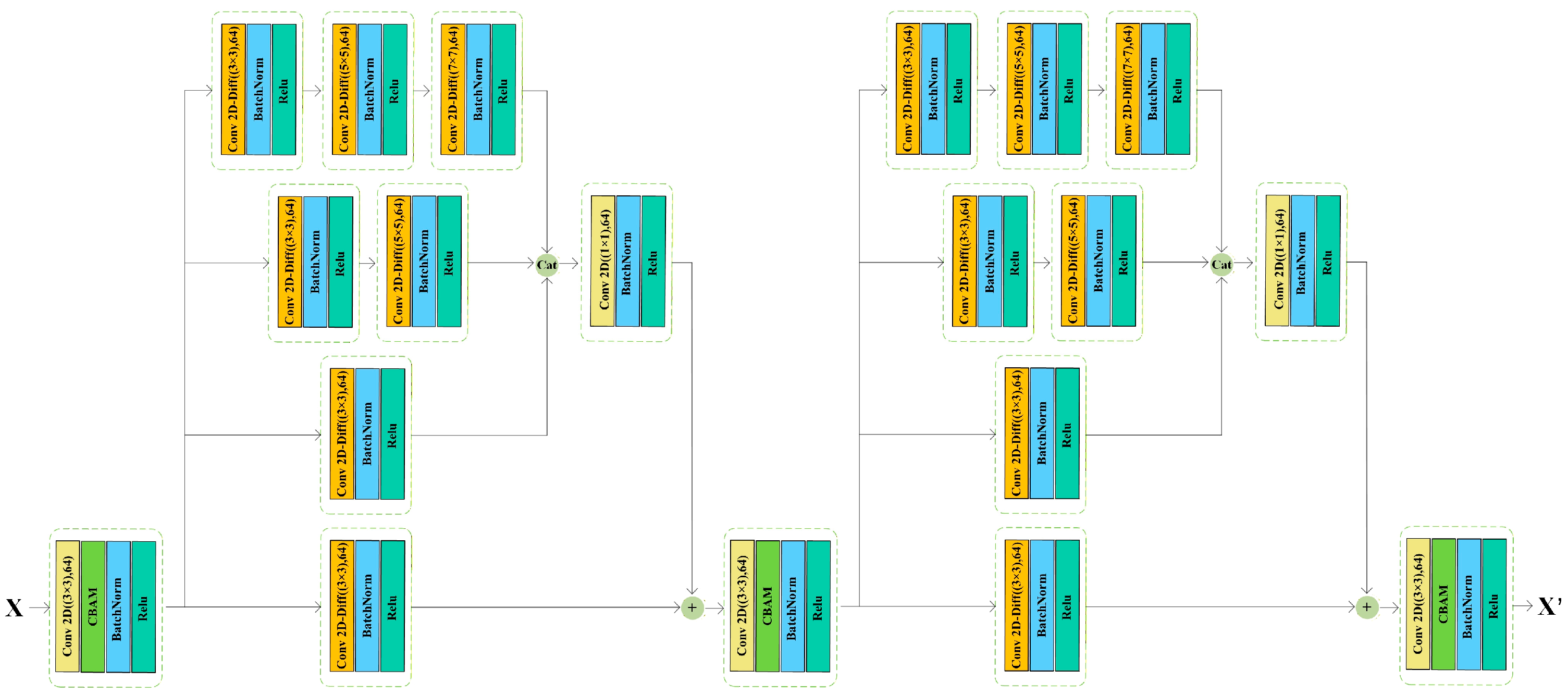
To improve the model’s ability in perceiving edge information and local contrast in HSI, we propose a multiscale differential convolutional residual module that combines standard 2D convolution with 2D differential convolution, as shown in Figure 3. Before applying 2D convolution to the feature maps obtained from the SSRE module, we first perform a Reshape operation. Due to the high channel dimensionality resulting from Reshape, we use a standard 3 × 3 2D convolution to decrease the channel dimension to 64 for initial feature extraction. The final output is generated by passing features through two multiscale differential convolutional residual modules. At the heart of this process is the MDRM, employing three parallel processing pathways to capture spatial characteristics across varying scales. The first branch applies a 3 × 3 differential convolution to capture fine-grained local details. The second branch introduces a parallel setup with 3 × 3 and 5 × 5 kernels, expanding the spatial receptive field. To further enrich the feature representation, the third branch incorporates a broader combination of 3 × 3, 5 × 5, and 7 × 7 convolutions, allowing the network to learn features with multiple levels of spatial granularity. These outputs are concatenated to integrate information from diverse receptive fields, enhancing the expressiveness of the learned features. A subsequent 1 × 1 convolution refines the fused representations, emphasizing local spatial cues. To preserve input characteristics and facilitate gradient propagation, a residual connection is introduced by element-wise summation between the first branch output and a parallel 1 × 1 convolution path. This design improves training stability, reduces gradient vanishing, and thereby strengthens the network’s ability to discern intricate spatial patterns. A final 3 × 3 convolution is employed to further distill high-level spatial information from the aggregated features. The resulting feature maps effectively integrate multi-scale information while preserving crucial structural details from the original input. To enhance the model’s nonlinear representation capacity and improve data fitting performance, we incorporate Batch Normalization layers and ReLU nonlinearities after every convolutional layer. Additionally, we implement CBAM attention mechanisms on three parallel 3 × 3 2D convolution branches to adaptively enhance the weights of both spatially significant regions and discriminative spectral features.

2.3.1. Two-Dimensional Differential Convolution

The 2D differential convolution enhances edge, texture, and local feature extraction by computing differential information between neighboring pixels. As illustrated in Figure 4, for an input image $I(x,y)$ and a convolutional kernel $K(i,j)$ with size (2k + 1) × (2k + 1), the conventional computation can be mathematically formulated as follows:

$$I_{out}(x,y)={\displaystyle \sum _{i=-k}^k{\displaystyle \sum _{j=-k}^{k}I(x+i,y+j)·K(i,j)}}$$

(1)

where $I(x+i,y+j)$ represents the pixel value of the input image, $K(i,j)$ denotes the convolutional kernel weights, and $I_{out}(x,y)$ indicates the output feature value. Unlike conventional convolution, the fundamental principle of differential convolution involves computing the difference between neighboring pixels and the central pixel, rather than directly utilizing the pixel values themselves. The mathematical formulation is expressed as follows:

$$I_{out}(x,y)={\displaystyle \sum _{i=-k}^k{\displaystyle \sum _{j=-k}^k(I(x+i,y+j)-I(x,y))·K(i,j)}}$$

(2)

The differential convolution operation, which computes inter-pixel differences, effectively enhances local texture information and accentuates spatial variations between different classes. This operation is particularly advantageous for discriminating similar categories in HSI. In HSI analysis, where class differentiation often relies on subtle spectral variations, the differential convolution mechanism amplifies these discriminative features, thereby significantly improving classification accuracy. Moreover, the computational process of differential convolution involves simple pixel difference operations, which demonstrates lower computational complexity compared to the weighted summation in conventional convolution. This characteristic makes it particularly suitable for large-scale hyperspectral data processing. To effectively leverage the complementary advantages of both differential and standard convolution, we introduce a learnable weighting factor α to achieve an adaptive balance between global context modeling and local feature enhancement. The mathematical formulation of the weighted central differential convolution is expressed as:

$$I_{out}(x,y)={\displaystyle \sum _{i=-k}^k{\displaystyle \sum _{j=-k}^k\begin{array}{l}[\alpha ·(I(x+i,y+j)-I(x,y))+\\ (1-\alpha )·I(x+i,y+j)]·K(i,j)\end{array}}}$$

(3)

where $\alpha$ controls the weight of differential information. When $\alpha$ = 0, the computation degenerates to standard convolution, focusing solely on global feature learning; when $\alpha$ = 1, it utilizes only central differential information, emphasizing local edge and detail features; when 0 < $\alpha$ < 1, this method effectively combines global contextual information with localized characteristics, thereby significantly improving the network’s feature representation capability. In practice, the learnable parameter α remains stable during training and typically converges to an intermediate value rather than collapsing to 0 or 1, indicating that both standard convolution and differential convolution contribute meaningfully to the final feature representation.

Although 2D differential convolution can be regarded as a constrained form of standard convolution, the imposed structural constraint introduces a useful inductive bias for hyperspectral image analysis. By explicitly encoding local intensity differences rather than relying entirely on learned filter weights, differential convolution strengthens the model’s sensitivity to spatial variations and fine boundary transitions. This is particularly aligned with the characteristics of hyperspectral data, where class distinctions often appear as subtle spectral–spatial changes rather than strong texture cues. The differential structure therefore guides the network toward emphasizing these discriminative variations, improving robustness under limited training samples and reducing the risk of overfitting. As a result, this design often yields clearer edge responses and more reliable boundary representation than unconstrained standard convolution in HSI classification tasks.

2.3.2. CBAM Modules

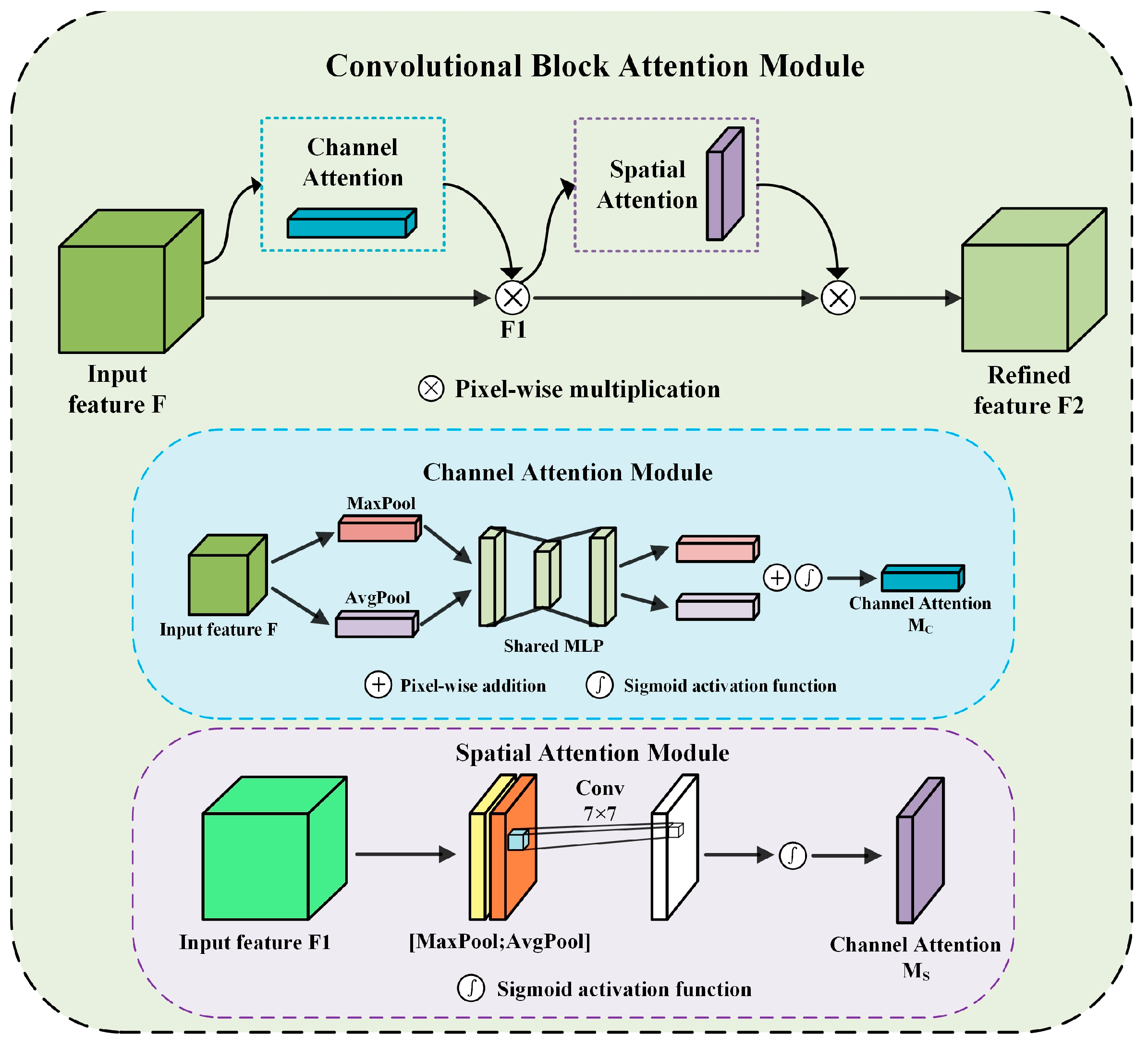
To amplify the significance of pivotal spatial–spectral features, this study incorporates the CBAM attention mechanism into three standard 3 × 3 2D convolutional layers [54]. As illustrated in Figure 5, the CBAM architecture primarily comprises two sequential sub-modules: the Spatial Attention Module (SAM) and the Channel Attention Module (CAM). First, the input feature F passes via CAM to compute channel-wise importance weights, generating weighted feature F1 to highlight key channels. Then, F1 is processed by SAM to calculate spatial importance, producing final feature F2 through pixel-wise weighting to emphasize critical regions. By combining both attention mechanisms, CBAM effectively enhances feature learning in deep neural networks, improving performance for classification, detection, and segmentation tasks. The computation is defined as:

$$\begin{array}{l}{F}_1=M_C·F\\ F_2=M_S·F_1\end{array}$$

(4)

In the equations, $F$ represents the input feature map, $M_C$ signifies the generated channel attention vector, $M_S$ is the produced spatial attention vector, while $F_1$ and $F_2$ correspond to the intermediate and final output features, respectively. The channel attention module operates through the following procedure: First, it generates two complementary global descriptors by performing parallel average and max pooling operations across the channel axis of the input feature map F. These descriptors then undergo a nonlinear transformation through a shared two-layer MLP. The transformed features are combined via element-wise summation to integrate global information. Finally, a sigmoid activation function normalizes the combined features to produce channel attention coefficients $M_C$. These coefficients subsequently recalibrate the weights of the input features along the channel dimension, producing the improved feature map F1. The computation is formulated as:

$$M_C=\sigma (\mathrm{MLP}(F_{\mathrm{avg}}^C)+\mathrm{MLP}(F_{\max }^C))$$

(5)

where σ denotes the sigmoid nonlinearity that projects the attention values into the normalized range [0, 1]. The shared MLP consists of fully connected neural network layers, with $F_{\max }^C$ and $F_{\mathrm{avg}}^C$ denoting the aggregated features from max-pooling operations and average-pooling, respectively, which ultimately produces the channel attention vector $M_C$. The spatial attention mechanism functions through the following computational process: First, it applies both average pooling and max pooling along the channel axis of the channel-enhanced feature $F_1$, producing two single-channel feature maps to capture different types of spatial information. These features are channel-wise concatenated and processed by a 7 × 7 convolution to extract local spatial relationships. Finally, a sigmoid activation function generates the spatial attention weights $M_S$, which are applied to $F_1$ through pixel-wise multiplication to produce the final enhanced feature $F_2$, thereby improving the model’s focus on target regions. The computation is formulated as:

$$M_{\mathrm{s}}=\sigma (C{\mathrm{onv}}_{7\times 7}([F_{\mathrm{avg}}^S,F_{\max }^S]))$$

(6)

where σ indicates the sigmoid nonlinear transformation, Conv7 × 7 represents the 7 × 7 convolutional operator; $F_{\mathrm{avg}}^S$ and $F_{\max }^S$ denote the spatially aggregated features from average- and max-pooling, respectively, and $M_{\mathrm{s}}$ is the final generated spatial attention vector. In contrast to more elaborate attention mechanisms such as SE-Net and Non-Local blocks, CBAM was adopted for its compact architecture and its capacity to concurrently capture both spatial and channel-level information. This characteristic makes it well-suited for hyperspectral image classification, where data are highly dimensional yet annotated samples are scarce. By adaptively enhancing salient spectral–spatial responses with negligible computational cost, CBAM achieves an effective compromise between representational power and model efficiency.

2.4. Transformer Branch

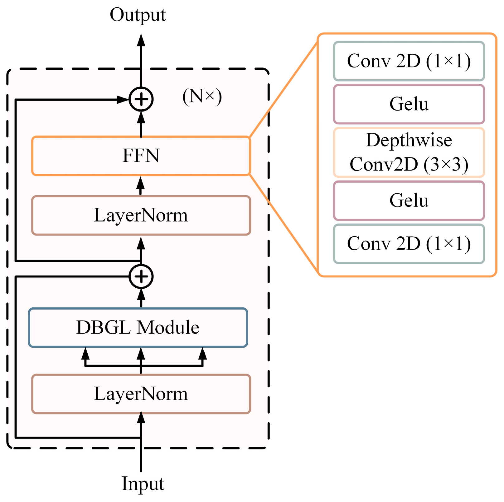
As demonstrated in Figure 6, the Transformer branch comprises N identical encoder layers. Each encoder contains two key modules: the DBGL module and FFN, which significantly enhance the capacity for joint global–local spatial–spectral feature extraction. We incorporate normalization layers within each encoder to improve numerical stability by normalizing feature distributions across samples, thereby enabling more effective weight computation in subsequent attention mechanisms. Given input data I1, the encoder can be formally expressed as:

$$\begin{array}{l}{\mathrm{P}}_1=\mathrm{DBGL}(\mathrm{LN}({\mathrm{I}}_1))+{\mathrm{I}}_1\\ {\mathrm{P}}_2=\mathrm{FFN}(\mathrm{LN}({\mathrm{P}}_1))+{\mathrm{P}}_1\end{array}$$

(7)

where LN denotes Layer Normalization, ${\mathrm{P}}_1$ denotes the output generated by applying residual connection between the DBGL-processed features and the original input ${\mathrm{I}}_1$, and ${\mathrm{P}}_2$ corresponds to the output produced through residual connection between the FFN-processed features and input ${\mathrm{P}}_1$. The architectural details of the DBGL module and FFN module will be elaborated in subsequent sections.

2.4.1. DBGL Module

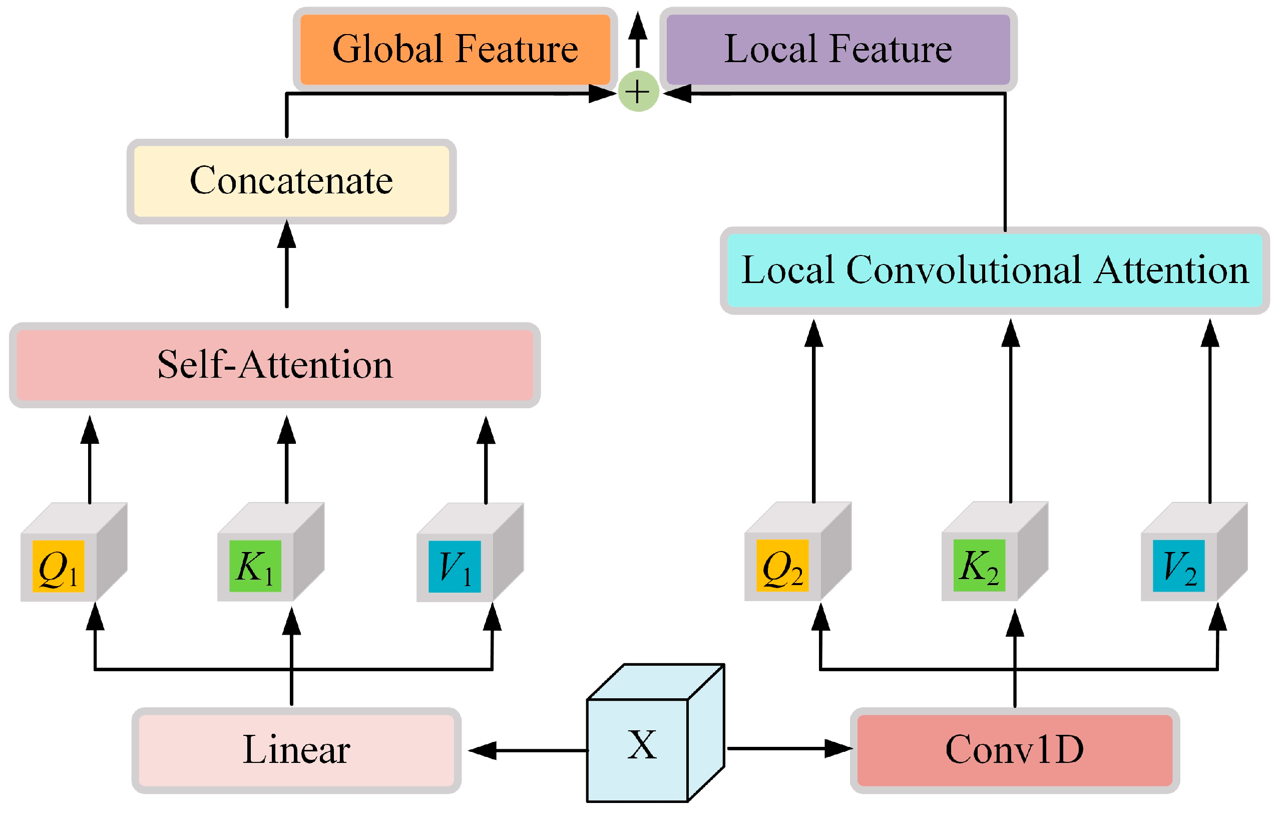
The DBGL module employs standard self-attention for global feature extraction and convolutional operations for local feature enhancement through QKV computation, ultimately fusing local and global information to advance hyperspectral classification accuracy. As shown in Figure 7, the DBGL module primarily comprises two parallel branches. The first branch computes $Q_1$, $K_1$, and $V_1$ through linear transformations, then utilizes Self-attention modules for modeling global contextual dependencies from hyperspectral data. The computational process of this branch is formulated as:

$$\begin{array}{l}{Q}_1=W_{Q_1}X,K_1=W_{K_1}X,V_1=W_{V_1}X\\ O_{\mathrm{SA}}=W_O(\mathrm{Concat}(\mathrm{softmax}({\displaystyle \frac{Q_1{K}_1^T}{\sqrt{D_h}}}){\mathrm{V}}_1))\end{array}$$

(8)

In the equation, X denotes the input feature map, $W_{Q_1}$, $W_{K_1}$, and $W_{V_1}$ represent trainable parameter matrices for projecting $Q_1$, $K_1$, and $V_1$, respectively. The term $\sqrt{D_h}$ serves as a scaling factor to stabilize gradients. Softmax indicates the normalization operation, while Concat refers to the concatenation operation. $W_O$ represents the output projection weight matrix that merges the multi-head attention results back to the original dimension, and $O_{\mathrm{SA}}$ signifies the output feature obtained from the standard self-attention branch. The second branch computes $Q_2$, $K_2$, and $V_2$ through 1D convolution, then employs a local convolutional attention mechanism to enhance spatial local features in hyperspectral data. The use of 1D convolution instead of 2D convolution is primarily driven by the need to capture long-range spectral dependencies across different spectral bands, which is critical in hyperspectral imaging. While 2D convolutions are designed to model spatial features, 1D convolutions are more suitable for capturing spectral relationships, enabling the model to better distinguish spectral variations between materials. This is particularly beneficial in hyperspectral data, where spectral information plays a key role in differentiating materials with similar spatial structures but distinct spectral signatures. The computational formula for this branch is as follows:

$$\begin{array}{l}{Q}_2=\mathrm{Conv}1\mathrm{D}(X),K_2=\mathrm{Conv}1\mathrm{D}(X),\\ V_2=\mathrm{Conv}1\mathrm{D}(X)\\ O_{\mathrm{conv}}=\mathrm{softmax}({\displaystyle \frac{Q_2{K}_2^T}{\sqrt{D_h}}})V_2\end{array}$$

(9)

where $X$ denotes the input feature map, Conv1D represents the 1D convolutional operation with a 3 × 3 kernel for local receptive field feature extraction, Softmax indicates the normalization operation, and Oconv corresponds to the output features from the local convolutional attention branch. The final output is obtained through weighted summation of both branches’ results. This fusion strategy enables simultaneous learning of local texture information and large-scale global context, effectively compensating for the potential limitation of self-attention mechanisms that may over-emphasize the current position when encoding positional information. The fusion computation is formulated as:

$$O_{\mathrm{out}}=O_{\mathrm{SA}}+O_{\mathrm{conv}}$$

(10)

The proposed DBGL attention mechanism integrates the complementary advantages of self-attention and convolutional attention, allowing the network to model both long-range contextual relationships and subtle local variations within hyperspectral data. In contrast to conventional Transformer attention, which often underrepresents localized spatial structures, DBGL explicitly blends global and local cues to maintain spatial consistency and enhance robustness against spectral fluctuations—two persistent challenges in hyperspectral image classification.

2.4.2. FFN Module

The FFN module enhances feature representation capability by performing further transformations on features processed by the DBGL module, thereby improving the model’s nonlinear modeling capacity. As illustrated in Figure 6, the FFN architecture employs two sequential 1 × 1 convolutional layers followed by a 3 × 3 depthwise separable convolution, with Gelu activation functions incorporated between layers to increase nonlinearity. First, the input features undergo channel-wise projection via a 1 × 1 convolution to decrease computational complexity and advance efficiency. The Gelu activation function is then applied for the first nonlinear transformation to enhance feature representation. Gelu is preferred over Relu due to its smoother nonlinear activation, which mitigates the vanishing gradient problem and the issue of neuron deactivation that can arise with Relu, particularly in deeper networks. This characteristic contributes to more stable training dynamics and improves the gradient flow during backpropagation. Subsequently, a 3 × 3 depthwise separable convolution extracts local spatial information, enabling more effective learning of local characteristics in hyperspectral data. Following this, the second Gelu activation further strengthens nonlinear mapping capability for better learning of complex patterns. Finally, the second 1 × 1 convolution restores the feature dimensionality, ensuring the FFN output maintains the same shape as the input for subsequent residual connections. Given input data Pin, the FFN operation can be expressed as:

$${\mathrm{P}}_{\mathrm{FFN}}{ = \mathrm{Conv}2\mathrm{D}}_{1\times 1}{(\mathrm{DWConv}2\mathrm{D}}_{3\times 3}{(\mathrm{Conv}2\mathrm{D}}_{1\times 1}({\mathrm{P}}_{\mathrm{in}})\left)\right)$$

(11)

where Conv2D1 × 1 denotes a 2D convolutional operation employing 1 × 1 kernels, DWConv2D3 × 3 represents a 2D depthwise separable convolution utilizing 3 × 3 kernels, and PFFN indicates the output features after FFN processing.

3. Experimental

3.1. Datasets

To evaluate the efficiency of the suggested HSIC method, this paper conducts comprehensive experiments on three extensively used benchmark hyperspectral datasets: Salinas, Pavia University, and Indian Pines. The detailed specifications of these datasets are summarized in

Table 1. Ground truth classes for the three HSI datasets.

Indian Pines (IP)				Pavia University (PU)			Salinas (SA)
No.	Category	Color	Sample	Category	Color	Sample	Category	Color	Sample
1	Alfalfa		46	Asphalt		6631	Broccoli-green-weeds_1		2009
2	Corn-notill		1428	Meadows		18,649	Broccoli-green-weeds_2		3726
3	Corn-mintill		830	Gravel		2099	Fallow		1976
4	Corn		237	Trees		3064	Fallow-rough-plow		1394
5	Grass-pasture		483	Painted metal sheets		1345	Fallow-smooth		2678
6	Grass-trees		730	Bare soil		5029	Stubble		3959
7	Grass-pasture-mowed		28	Bitumen		1330	Celery		3579
8	Hay-windrowed		478	Self-blocking bricks		3682	Grapes-untrained		11,271
9	Oats		20	Shadows		947	Soil-vineyard-develop		6203
10	Soybean-notill		972				Corn-senesced-green-weeds		3278
11	Soybean-mintill		2455				Lettuce-romaine-4wk		1068
12	Soybean-clean		593				Lettuce-romaine-5wk		1927
13	Wheat		205				Lettuce-romaine-6wk		916
14	Woods		1265				Lettuce-romaine-7wk		1070
15	Buildings-Grass-Trees-Drivers		386				Vineyard-untrained		7268
16	Stone-Steel-Towers		93				Vineyard-vertical-trellis		1807

.

3.1.1. Indian Pines Dataset

This dataset, serving as the inaugural benchmark for HIC, was collected using the AVIRIS sensor over a pine forest in northwestern Indiana, USA. This dataset includes 16 land-cover classes with an original spectral resolution of 220 bands. Following the elimination of 20 bands impacted by water vapor absorption, the subsequent analysis was conducted using the remaining 200 spectral channels. The spatial dimensions of the image are 145 × 145 pixels (totaling 21,025 pixels), among which 10,776 background pixels were excluded from classification, resulting in 10,249 valid pixel samples for ground-truth analysis.

3.1.2. Pavia University Dataset

It was acquired using the ROSIS sensor at the University of Pavia, Italy. The dataset comprises a 610 × 340 pixel image containing 42,776 valid ground object pixels, with their categorical distribution detailed in

Table 2. Overview of representative hyperspectral image classification models used for comparison.

Category	Model/Reference	Core Technique	Strengths	Limitations
Traditional ML	SVM [17], RF [18]	Handcrafted features with kernel-based classification	Simple, interpretable, effective on small datasets	Poor generalization on high-dimensional data
CNN-based	2D-CNN [27], 3D-CNN [30], HybridSN [31]	Local spectral–spatial feature extraction via convolution	Strong local modeling, stable training	Limited receptive field, lacks global context
Transformer-based	ViT [35], LESS-Former [40], S2CABT [41]	Global dependency modeling via self-attention	Captures long-range spectral relations	Requires large labeled data, weak spatial detail
Hybrid CNN–Transformer	HiT [46], SSFTT [55], TransHSI [47]	Combines convolutional and attention mechanisms	Better integration of local/global cues	Fusion strategy often shallow or computationally heavy
Proposed	STM-Net (Ours)	Multi-scale spectral–spatial fusion via SSRE, MDRM, DBGL	Balanced efficiency and accuracy; strong feature representation	—

. Following the elimination of 12 bands with significant noise, the remaining 103 spectral bands were retained for subsequent experimental analysis. The curated dataset encompasses 9 distinct land cover categories.

3.1.3. Salinas Dataset

It was acquired using the AVIRIS imaging spectrometer in Pasadena, CA, USA. The hyperspectral image comprises 512 × 217 pixels, with each pixel representing a 3.7 m ground resolution. A total of 16 distinct land cover categories are included, accounting for 54,129 labeled samples. Following radiometric calibration, 204 spectral bands were selected for further analysis.

3.2. Experimental Settings

3.2.1. Implementation Details

For each dataset, 10% of the labeled samples from each class were randomly selected for training, and the remaining samples were used for testing. To ensure a fair comparison, the same data partitions were applied to all competing methods. Given the limited number of labeled samples in hyperspectral datasets, model evaluation was carried out directly on the test set after training. All experiments are conducted on a laptop equipped with a 13th Gen Intel^® Core™ i5-13490F processor, 32.0 GB RAM, and an NVIDIA GeForce RTX 4060 Ti GPU under Windows 11. The implementation utilizes Pytorch 1.13.1 and Python 3.7. To ensure statistical reliability, each experiment is repeated 10 times with averaged results reported.

3.2.2. Evaluation Metrics

For a quantitative evaluation of the performance of the proposed STM-Net and baseline approaches, three established assessment criteria were adopted: Kappa coefficient, Average Accuracy (AA), and Overall Accuracy (OA). These metrics effectively measure classification performance, where higher values indicate better classification results.

3.3. Parameter Sensitivity Analysis

Given the critical impact of hyperparameters on model performance, we systematically optimized the most influential hyperparameters to ensure robustness and generalization capability. The proposed network was trained for 100 epochs, utilizing a learning rate of 0.001 and a batch size of 128. The Adam optimizer was employed for model training with the following settings: β1 = 0.9, β2 = 0.999, epsilon = 10⁻⁸, and no weight decay was applied. Additionally, we used a cosine annealing learning rate schedule, starting with an initial learning rate of 0.001 and dynamically adjusting it during training. A cross-entropy loss function was employed for network optimization. The Adam optimizer was employed for model training along with a cross-entropy loss function for network optimization. Furthermore, we conducted detailed analyses on key hyperparameters including channel numbers and spatial input dimensions to further enhance classification performance

3.3.1. Channel Number Analysis

In HIC tasks, PCA is widely used to reduce spectral dimensionality, lowering computational cost and removing redundancy. Too many channels cause redundant features and higher overhead, while too few risk losing vital information and reducing accuracy. To find the optimal number, experiments tested channel counts of 20, 25, 30, 35, and 40 on three public hyperspectral datasets. Figure 8 demonstrates that the classification accuracy for all 3 datasets initially improves and subsequently declines with the growing number of reduced-dimensional features, which demonstrates the critical importance of appropriate channel selection for optimal performance. For the IP dataset, the AA, OA, and Kappa values all peak at 30 channels, indicating the model’s optimal balance between feature utilization and information redundancy avoidance. Experimental results indicate that both the PU and SA datasets attain peak classification accuracy when configured with 25 spectral channels.

3.3.2. Spatial Input Dimension

This study employs a neighborhood extraction approach, where all pixels within a defined neighborhood are processed as a sample patch for model input. The spatial dimension of these patches significantly impacts classification performance: undersized patches may lead to insufficient contextual information for effective feature extraction, while oversized patches could introduce excessive irrelevant data, increasing computational complexity and potentially degrading accuracy. Consequently, optimal selection of spatial dimensions is crucial for model performance optimization. To systematically investigate this, we performed a comprehensive experimental study on three benchmark hyperspectral datasets using sample patches of 19 × 19, 21 × 21, 23 × 23, 25 × 25, and 27 × 27 pixels for comparative analysis. This study explores how spatial input dimensions affect HIC, aiming to identify optimal settings. As shown in Figure 9, the SA and IP datasets reached peak OA, AA, and Kappa scores at a 23 × 23 window, while PU performed best at 21 × 21, highlighting the importance of sufficient spatial context for effective feature learning. These findings emphasize the need to tailor spatial dimensions to dataset characteristics to enhance feature extraction and generalization for reliable classification.

3.4. Comparative Experiment Analysis

To better contextualize the proposed approach, we first summarize in Table 2 the representative models employed in our benchmark experiments. These include classical machine learning algorithms, convolution-based deep learning models, and hybrid CNN–Transformer frameworks that combine local feature extraction and global context modeling. The table outlines the core techniques, strengths, and limitations of these representative approaches, providing a concise overview of the methodological landscape and clarifying the motivation for developing a more balanced and efficient spectral–spatial framework.

As shown in Table 2, most existing models emphasize either local spatial–spectral features or global contextual dependencies, but rarely achieve a well-balanced integration of both. The proposed STM-Net addresses this limitation through a unified hybrid architecture that combines CNN-based fine-grained local feature extraction with Transformer-based long-range context modeling, thereby improving spectral–spatial representation while maintaining computational efficiency. Models such as HiT (2022), SSFTT (2023), and TransHSI (2023) represent recent state-of-the-art CNN–Transformer architectures in hyperspectral image classification. The proposed STM-Net is designed to achieve more efficient spectral–spatial integration while maintaining competitive accuracy and lower computational complexity.

The generalization ability and classification performance of the proposed model were evaluated through comparative experiments on three widely used hyperspectral datasets: IP, PU, and SA. The model’s performance was benchmarked against several established methods, including traditional machine learning (e.g., SVM [17]) and deep learning approaches (e.g., 2D-CNN [27], 3D-CNN [30], HybridSN [31], and ViT [35]). Additionally, hybrid models such as SSFTT [55] and HiT [46], which integrate CNN and Transformer architectures, were considered. To ensure fair comparisons, all models were trained under identical conditions: a batch size of 128, 100 training epochs, and spatial patch sizes optimized according to their respective original studies. Results were averaged over 10 independent runs to ensure statistical robustness.

3.4.1. Quantitative Analysis

Table 3. Classification results of different algorithms on the IP dataset.

Classes	SVM	2D-CNN	3D-CNN	HybridSN	ViT	SSFTT	HiT	STM-Net
1	93.75	80.65	100	100	78.65	96.15	97.06	97.62
2	81.08	99.59	99.18	99.27	90.17	98.96	98.97	99.06
3	82.26	97.19	96.19	94.43	81.37	98.15	98.14	97.37
4	84.57	99.53	100	100	100	100	99.53	100
5	78.35	100	95.19	98.15	91.92	97.51	100	98.62
6	91.97	98.92	97.9	98.35	98.8	99.09	98.94	99.85
7	100	96.15	90.48	96.15	72.97	96.15	96.15	100
8	97.26	96.85	97.29	98.17	91.38	96.41	98.17	100
9	82.61	100	100	88.89	100	100	100	100
10	93.26	98.99	93.44	98.18	92.13	98.17	96.95	98.16
11	81.07	93.38	96.58	96.86	87.6	97.65	97.95	98.61
12	76.04	94.93	96.49	97.37	94.2	97.56	98.65	99.43
13	91.04	100	100	100	91.71	100	100	100
14	94.64	99.65	98.68	99.2	94.72	99.82	99.91	99.3
15	98.2	93.28	99.11	100	97.75	98.82	98.55	100
16	59.86	97.18	97.56	100	88.37	98.68	93.98	92.13
OA (%)	86.27	96.99	97.13	97.92	90.73	98.36	98.53	98.86
AA (%)	87.98	96.64	97.38	97.81	88.32	98.32	98.31	98.76
K × 100	85.56	96.56	96.72	97.62	89.37	98.13	98.32	98.71

,

Table 4. Classification results of different algorithms on the PU dataset.

Classes	SVM	2D-CNN	3D-CNN	HybridSN	ViT	SSFTT	HiT	STM-Net
1	87.57	95.73	99.05	99.75	93.48	99.82	99.8	99.95
2	95.81	100	99.98	100	99.69	99.97	99.97	99.96
3	86.22	100	97.35	98.14	97.56	99.5	99.95	100
4	95.64	96.72	97.91	96.93	98.95	99.6	98.85	99.46
5	98.92	100	99.18	99.18	90.64	100	100	100
6	97.36	99.85	99.58	99.76	97.31	100	99.71	100
7	93.35	99.63	94.91	100	78.09	100	100	99.83
8	83.1	91.85	97.21	97.05	74.58	96.44	98	99.61
9	75.29	96.89	98.73	99.04	100	100	99.88	100
OA (%)	92.7	98.25	99.06	99.32	94.44	99.59	99.66	99.9
AA (%)	90.36	97.85	98.21	98.87	92.26	99.48	99.57	99.87
K × 100	92.05	97.67	98.75	99.1	92.6	99.46	99.55	99.88

and

Table 5. Classification results of different algorithms on the SA dataset.

Classes	SVM	2D-CNN	3D-CNN	HybridSN	ViT	SSFTT	HiT	STM-Net
1	98.64	100	100	100	100	100	100	100
2	95.72	100	100	100	99.88	100	100	100
3	91.78	100	100	100	100	100	100	100
4	93.12	100	100	98.43	96.21	94.65	100	100
5	95.24	95.22	92.87	99.75	99.67	99.87	98.77	100
6	100	97.22	99.94	99.75	100	100	100	99.55
7	99	100	100	100	100	100	100	100
8	92.72	96.68	99.98	99.34	96.16	99.7	99.99	99.97
9	98.98	99.8	100	100	99.96	99.95	100	99.98
10	98.54	99.9	99.46	99.9	99.97	100	99.97	100
11	97.49	93.66	98.77	99.9	100	100	99.69	100
12	100	95.52	99.48	98.52	94.45	99.94	100	100
13	96.44	98.66	100	96.27	95.65	100	100	100
14	95.89	95.68	100	100	76.69	100	100	100
15	86.69	99.79	98.17	99.85	99.5	100	100	100
16	97.55	99.62	100	100	99.94	100	99.94	100
OA (%)	94.95	98.36	99.29	99.64	97.27	99.78	99.93	99.96
AA (%)	95.99	98.23	99.29	99.48	96.13	99.63	99.9	99.97
K × 100	94.48	98.17	99.2	99.6	96.96	99.75	99.92	99.95

summarize the AA, OA, and Kappa coefficients achieved by various algorithms on the IP, PU, and SA datasets. The top-performing results for each metric are indicated in bold. Across all three datasets, the proposed STM-Net consistently delivers superior classification results, outperforming all baseline methods in terms of OA, AA, and Kappa, which highlights its robustness and strong generalization capacity. Specifically, STM-Net achieves steady performance gains on every dataset. On the IP dataset, the suggested method outperforms HiT (the second-best approach) with relative improvements of 0.21% in OA, 0.55% in AA, and 0.39% in the Kappa coefficient. Comparable improvements are observed on the SA dataset, with respective increases of 0.19%, 0.34%, and 0.2%. Remarkably, within the PU dataset, STM-Net exhibits an outstanding Kappa coefficient of 99.88%, the outcomes are comparable to or surpass the most advanced existing methodologies. The empirical outcomes robustly validate the model’s efficiency across a range of hyperspectral imaging scenarios. An examination of category-specific performance reveals STM-Net’s superior classification accuracy in 9 of 16 categories within the IP dataset, highlighting its robustness across the board and its proficiency in identifying minority classes. The model is designed for datasets with imbalanced classes, where handling spectral variability and limited samples is challenging. Deep learning methods outperform traditional SVMs by effectively integrating spectral and spatial information. Notably, 2D-CNN and 3D-CNN differ in performance, both excel at local feature extraction but struggle with capturing global dependencies. While ViT and similar Transformers excel at modeling long-range dependencies, they struggle with fine-grained spatial details, which can reduce classification accuracy for certain categories. This highlights the need to balance local and global feature representation. Hybrid models like HiT and SSFTT address this by combining CNN and Transformer architectures. STM-Net advances this approach, consistently achieving higher OA, AA, and Kappa scores across datasets. By combining the local feature extraction of the CNN with the global modeling of the Transformer, it enhances spectral–spatial fusion. Notably, STM-Net improves AA, especially for underrepresented classes, and surpasses 99% in OA and Kappa on PU and SA datasets, showing strong generalization. Even amid performance saturation on PU, STM-Net maintains a competitive edge, demonstrating its capacity to extract more discriminative features and adapt reliably to complex hyperspectral tasks.

3.4.2. Qualitative Analysis

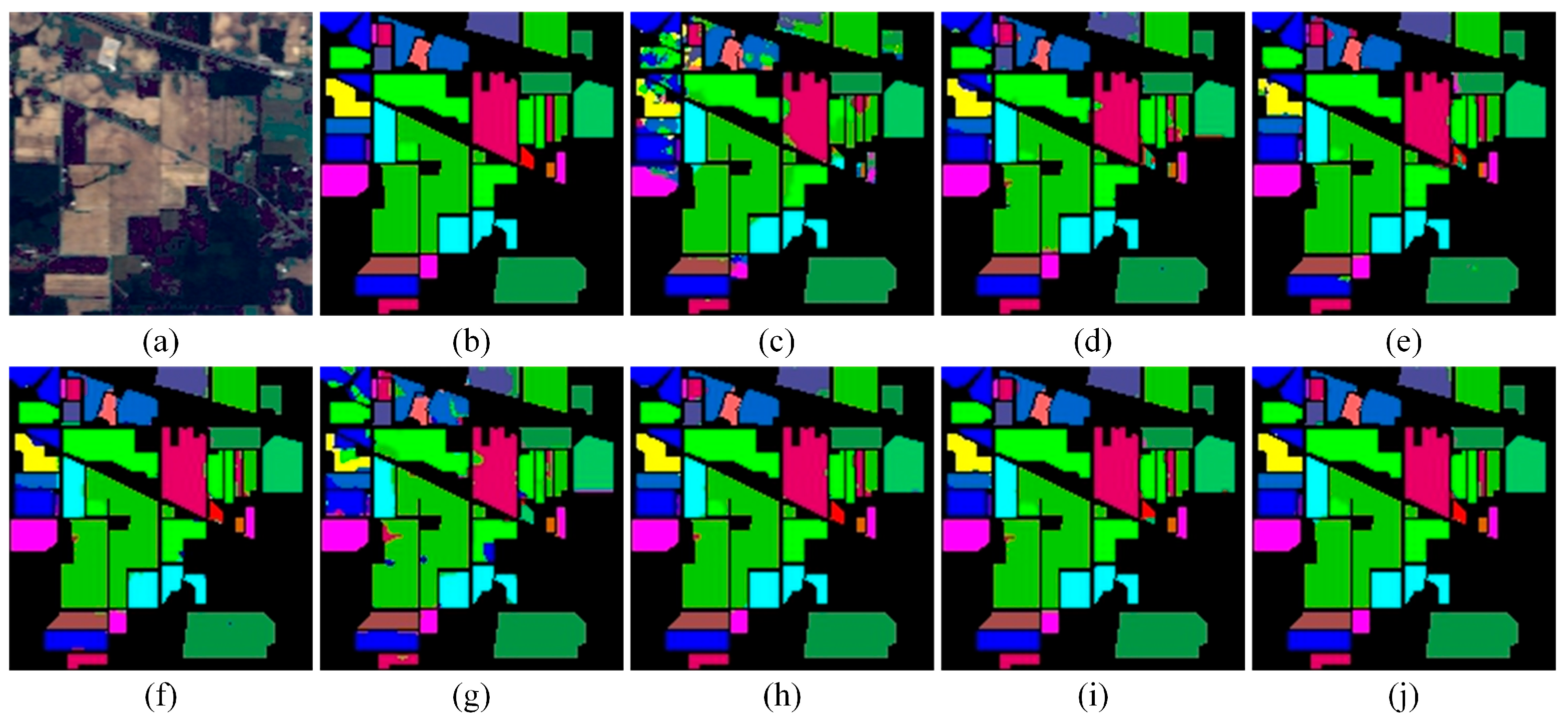
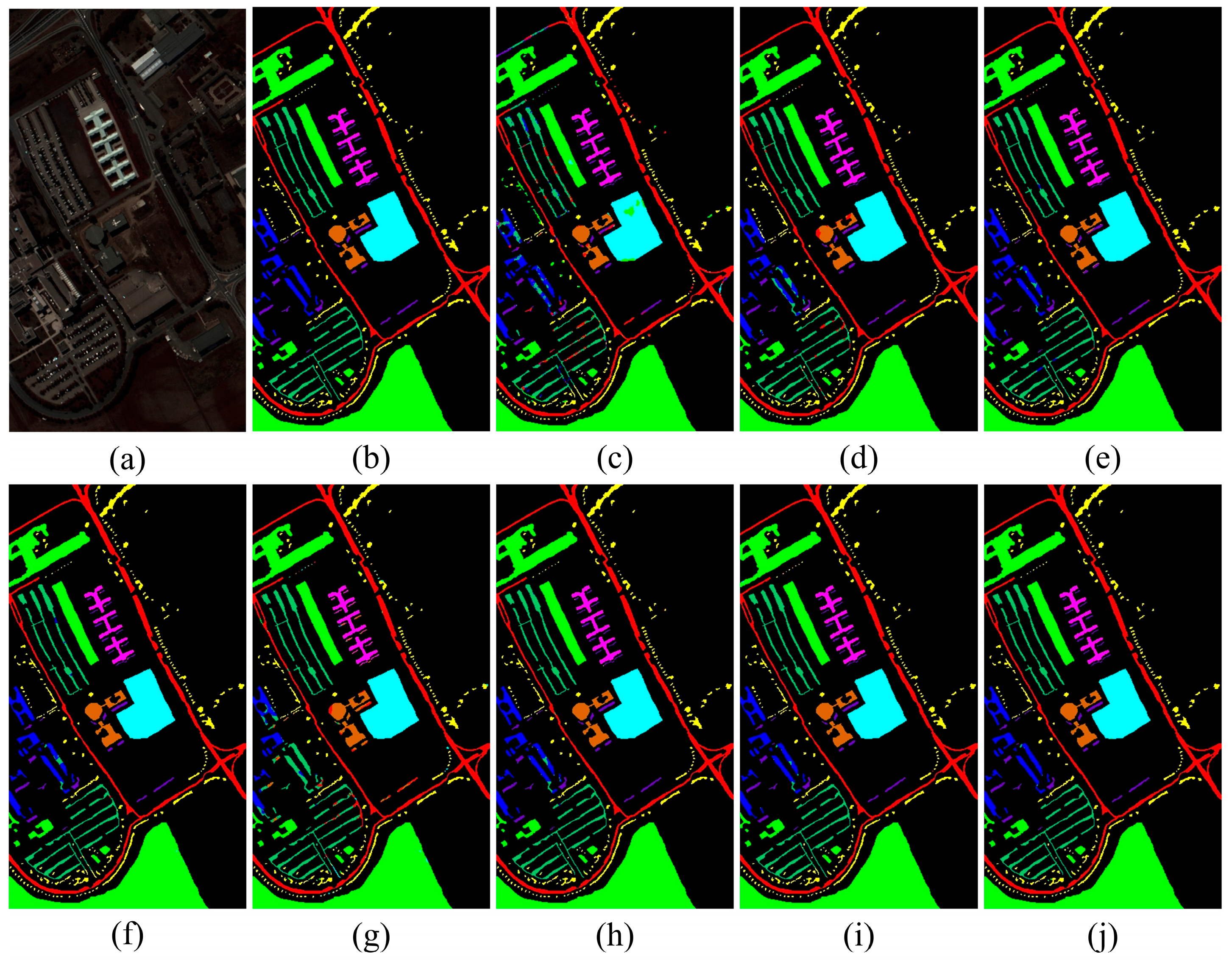
Figure 10, Figure 11 and Figure 12 present classification maps from STM-Net and baseline models on the IP, SA, and PU datasets, enabling visual comparison. STM-Net consistently delivers clearer class boundaries, reduced noise in homogeneous areas, and finer spatial details. Its outputs closely align with ground truth, mainly in areas with subtle spectral variations and mixed pixels. Visual enhancements are evident across diverse landscape scenarios, thereby bolstering the model’s dependability and versatility in various hyperspectral imaging applications. Several factors influence these outcomes, including the complexity of land cover types, the distinctness of class boundaries, and the degree of spectral similarity between classes. For example, SVM—relying solely on spectral features—struggles with spectral mixing effects, resulting in considerable misclassification and noisy predictions, especially near class boundaries. Although 2D-CNN and 3D-CNN incorporate spatial information and improve accuracy to some extent, they often exhibit fragmentation in class boundaries and difficulty in identifying minority classes, particularly in the IP and SA datasets. HybridSN, which merges 2D and 3D CNNs, achieves better performance in large uniform regions but continues to show confusion in spectrally similar small classes. The ViT model, while capable of modeling long-range dependencies through its Transformer-based structure, lacks sufficient local detail modeling, which limits its accuracy near boundaries. Hybrid methods like SSFTT and HiT—combining CNNs and Transformers—demonstrate stronger capacity for joint spectral–spatial modeling, achieving improved results in certain categories such as buildings and roads in the PU and SA datasets. However, they still face challenges in the IP dataset, including confusion between fine-grained categories and scattered misclassifications. Conversely, STM-Net outperforms all comparative methods across datasets, delivering cleaner, more accurate classification maps. On IP, it reduces pixel-level noise and sharpens boundaries; on PU, it achieves perfect accuracy in several classes with boundary predictions closely matching the ground truth; and on SA, it effectively detects small classes while minimizing confusion. These results highlight STM-Net’s architecture, which combines CNNs’ local feature extraction with Transformers’ global context modeling, leading to superior segmentation, boundary clarity, and generalization.

3.4.3. Complexity Analysis

To systematically assess the computational efficiency and resource requirements of different models for HIC tasks, we conducted a comprehensive comparison of floating-point operations (FLOPs) and model parameters (Params), with detailed results on the IP dataset presented in

Table 6. Analysis results of model complexity.

Methods	Params (M)	Flops (GB)
2D-CNN	1.88	0.03
3D-CNN	2.53	0.21
HybridSN	5.12	0.25
ViT	0.69	0.12
SSFTT	0.62	0.02
HiT	21.23	4.29
STM-Net	1.92	0.95

. The comparative methods included traditional convolutional architectures (2D-CNN, 3D-CNN), hybrid networks (HybridSN), Transformer-based models (ViT, SSFTT, HiT), and the proposed STM-Net model. As shown in the table, STM-Net contains 1.92 M parameters and requires 0.95 GB FLOPs. While its computational complexity is slightly higher than some lightweight models (e.g., SSFTT and ViT), it remains significantly lower than large Transformer models like HiT (21.23 M parameters, 4.29 GB FLOPs). Notably, STM-Net achieves optimal performance across all three-evaluation metrics (AA, OA, and Kappa coefficient), demonstrating its substantial advantages in classification accuracy. These results indicate that STM-Net achieves an excellent balance between model efficiency and classification performance. Compared to lightweight models with lower computational costs but inferior accuracy, as well as complex models with redundant parameters and excessive computational overhead, STM-Net exhibits strong potential for practical applications and considerable value for engineering deployment. The proposed architecture strikes a balance between accuracy and computational efficiency, rendering it well-tailored for practical hyperspectral image analysis. Its ability to deliver strong results with low resource demands supports its use in hardware-constrained or real-time applications.

3.5. Ablation Study Analysis

An ablation study on the IP dataset was performed to clarify the role of each STM-Net component. This involved systematically removing key modules, testing alternative Transformer setups, and exploring different MDRM structures. Performance changes were measured using OA, AA, and the Kappa coefficient. A consistent training setup across all variants ensured fair comparisons and accurate assessment of each architectural choice’s impact on classification performance.

3.5.1. Key Module Removal Experiments

Table 7. The key module removal experiment results.

Nets	Model Structure	OA	AA	Kappa
STM-Net (Baseline)	SSRE + MDRM + Transformer	98.86	98.76	98.71
(w/o SSRE)	MDRM + Transformer	97.44	97.33	97.08
(w/o MDRM)	SSRE + Transformer	98.24	98.15	98.01
(w/o Transformer)	SSRE + MDRM	98.56	98.45	98.39

shows that removing any key component (SSRE, MDRM, or Transformer) reduces performance on the IP dataset. Notably, excluding SSRE lowers OA by 1.42%, highlighting the value of its 3D convolutions for effective spectral–spatial feature extraction in complex category recognition. The OA drops by 0.62% when removing MDRM, indicating its role in enhancing local features through multi-scale differential convolution for boundary classification. A 0.3% OA reduction occurs without the Transformer module, highlighting its contribution to global feature modeling. These results show that SSRE contributes most significantly to classification performance, followed by MDRM and Transformer, with their combined integration achieving optimal results.

3.5.2. Transformer Branch Variant Experiments

As shown in

Table 8. The experimental results of transformer branch variant.

Nets	Transformer Structure	OA	AA	Kappa
STM-Net (Baseline)	DBGL	98.86	98.76	98.71
Vanilla Transformer	Global attention only	98.45	98.56	98.23
Local-Only	Local only convolution	98.49	98.42	98.28

, comparative analysis of the DBGL mechanism, standard Transformer (Vanilla Transformer), and Local-Only convolution reveals that DBGL achieves optimal classification performance. The Vanilla Transformer, which relies solely on global attention, shows a 0.41% decrease in OA and demonstrates poorer classification accuracy in boundary regions, indicating that exclusive dependence on global information inadequately captures local details. While the Local-Only approach enhances spatial feature extraction, its lack of global relationship modeling capability leads to reduced overall class discriminability. In contrast, DBGL effectively balances feature learning through global-local fusion, thereby improving both boundary classification accuracy and overall model stability.

3.5.3. MDRM Structure Variant Experiments

The ablation study results in

Table 9. The experimental results of structural variation in MDRM.

Nets	MDRM Structure	OA	AA	Kappa
STM-Net (Baseline)	Multiscale differential convolution + CBAM	98.86	98.76	98.71
(w/o CBAM)	Multiscale differential convolution	98.62	98.65	98.43
(w/o Multi-Scale)	Single scale difference convolution	98.36	98.16	98.13
(w/o DiffConv)	Ordinary 2D convolution	98.57	98.61	98.37

demonstrate that removing any component from the MDRM structure (CBAM, multi-scale convolution, or differential convolution) leads to performance degradation. Specifically, the OA decreases by 0.24% without CBAM, confirming its role in enhancing feature selection through attention mechanisms. The removal of multi-scale convolution results in a 0.5% OA reduction, highlighting the critical importance of multi-scale information for hyperspectral classification, particularly in boundary recognition. When eliminating differential convolution, a 0.29% OA drop occurs, demonstrating its effectiveness in improving local feature contrast and spatial discriminability. Model efficacy is most enhanced by multi-scale convolution, with differential convolution and CBAM also having a substantial impact. Upon integration, these components collectively elevate classification consistency and the model’s capacity for class boundary delineation.

4. Discussion

The experimental results demonstrate that STM-Net provides a more expressive and balanced representation of spectral–spatial information than competing approaches. The SSRE module plays a central role in this improvement. By employing multi-scale 3D convolutions with residual connections, SSRE captures informative spectral–spatial cues while reducing redundancy. The noticeable accuracy drop observed in its ablation verifies its importance in stabilizing feature extraction, especially under limited training samples.

Traditional CNN-based classifiers generally emphasize local texture and edge patterns but struggle to model long-range context, which is essential in hyperspectral imagery that often contains mixed pixels and spectrally similar categories. The incorporation of the DBGL mechanism addresses this limitation. Through the joint use of global self-attention and local convolutional attention, the Transformer branch becomes capable of capturing extended contextual relationships without sacrificing sensitivity to fine structural variations. The performance gains observed in boundary regions and minority classes further highlight the value of this global–local fusion strategy.

The MDRM also contributes substantially to the robustness of STM-Net. Its multi-scale differential convolutions, combined with CBAM attention, strengthen local contrast representation and texture discrimination. When either the multi-scale structure or the differential component is removed, the model exhibits a clear decline in accuracy, which underscores the importance of enhancing spatial detail for complex hyperspectral scenes.

The analysis of hyperparameters provides additional insights. Both PCA channel numbers and spatial window sizes exhibit dataset-dependent optimal values. Excessive spectral dimensions introduce redundant information, whereas overly small dimensions weaken class separability. Similarly, spatial windows must balance contextual completeness and noise suppression. These findings indicate that STM-Net benefits from a tailored configuration that corresponds to scene characteristics.

In summary, STM-Net achieves a strong balance between local feature extraction and global dependency modeling, while maintaining a manageable computational cost. Although the architecture is more complex than lightweight CNNs, it remains efficient enough for most remote sensing applications. Future research may incorporate model compression, semi-supervised or self-supervised strategies, and multimodal data fusion to further enhance adaptability in real-world operational environments.

5. Conclusions

This study introduces STM-Net, an innovative framework for HIC which synergistically merges the advantages of CNNs and Transformer architectures. The model incorporates three pivotal components—SSRE, MDRM, and DBGL—collectively enabling the efficient amalgamation of spectral and spatial attributes, while concurrently facilitating both local detail extraction and global context representation. The cohesive design manifests substantial enhancements in classification accuracy and generalization across diverse hyperspectral datasets. STM-Net outperforms baseline methods on the IP, SA, and PU datasets in AA, OA, and Kappa coefficient, demonstrating strong reliability and robustness. Ablation studies reveal that SSRE improves spectral–spatial feature extraction, MDRM enhances local structure and boundary detection, and DBGL expands contextual understanding. STM-Net also delivers sharper, more accurate classification maps. Future work may explore model compression, multimodal integration, and self-supervised learning to improve scalability. By integrating local feature learning with long-range dependency modeling, STM-Net offers an effective solution for complex hyperspectral classification.

References

1. Zhang, W.; Li, Z.; Li, G.; Zhuang, P.; Hou, G.; Zhang, Q.; Li, C. GACNet: Generate adversarial-driven cross-aware network for hyperspectral wheat variety identification. IEEE Trans. Geosci. Remote Sens. 2023, 62, 5503314. [Google Scholar] [CrossRef]
2. Stuart, M.B.; McGonigle, A.J.S.; Willmott, J.R. Hyperspectral imaging in environmental monitoring: A review of recent developments and technological advances in compact field deployable systems. Sensors 2019, 19, 3071. [Google Scholar] [CrossRef]
3. Zanotta, D.C.; Araújo, L.D.; De Souza, M.K.; Ibanez, D.M.; Silveira, L.G.; Veronez, M.R. Indirect calibration of hyperspectral images using rock samples. In Proceedings of the 14th Workshop on Hyperspectral Image and Signal Processing: Evolution in Remote Sensing (Whispers), Helsinki, Finland, 9–11 December 2024; pp. 1–5. [Google Scholar]
4. Nisha, A.; Anitha, A. Current Advances in Hyperspectral Remote Sensing in Urban Planning. In Proceedings of the 2022 Third International Conference on Intelligent Computing Instrumentation and Control Technologies (ICICICT), Kannur, India, 11–12 August 2022; pp. 94–98. [Google Scholar] [CrossRef]
5. Lee, S.; Namgoong, J.-M.; Kim, Y.; Cha, J.; Kim, J.K. Multimodal imaging of laser speckle contrast imaging combined with mosaic filter-based hyperspectral imaging for precise surgical guidance. IEEE Trans. Biomed. Eng. 2021, 69, 443–452. [Google Scholar] [CrossRef] [PubMed]
6. Zhang, D.; Sun, M. Multi-task joint 3D SWIN transformer learning for segmentation and classification of hyperspectral medicine images. In Proceedings of the IEEE International Conference on Acoustics, Speech and Signal Processing (ICASSP), Hyderabad, India, 6–11 April 2025; pp. 1–5. [Google Scholar]
7. Qi, J.; Gong, Z.; Xue, W.; Liu, X.; Yao, A.; Zhong, P. An unmixing-based network for underwater target detection from hyperspectral imagery. IEEE J. Sel. Top. Appl. Earth Observ. Remote Sens. 2021, 14, 5470–5487. [Google Scholar]
8. Chen, B.; Liu, L.; Zou, Z.; Shi, Z. Target detection in hyperspectral remote sensing image: Current status and challenges. Remote Sens. 2023, 15, 3223. [Google Scholar] [CrossRef]
9. Ding, J.; Li, X.; Zhao, L. CDFormer: A hyperspectral image change detection method based on transformer encoders. IEEE Geosci. Remote Sens. Lett. 2022, 19, 6015405. [Google Scholar] [CrossRef]
10. Zhao, H.; Lu, Z.; Sun, S.; Wang, P.; Jia, T.; Xie, Y.; Xu, F. Classification of large scale hyperspectral remote sensing images based on LS3EU-NET++. Remote Sens. 2025, 17, 872. [Google Scholar] [CrossRef]
11. Zhuang, J.; Chen, W.; Huang, X.; Yan, Y. Band selection algorithm based on multi-feature and affinity propagation clustering. Remote Sens. 2025, 17, 193. [Google Scholar] [CrossRef]
12. Qin, R.; Wu, B.; Liu, X.; Wu, Y. Hyperspectral image classification method based on global space-spectral attention mechanism. J. Shanghai Jiaotong Univ. (Sci.) 2024, early access. [Google Scholar] [CrossRef]
13. Li, B.; Wang, X.; Xu, H. SSRMamba: Efficient visual state space model for spectral super-resolution. In Proceedings of the IEEE International Conference on Acoustics, Speech, and Signal Processing (ICASSP), Hyderabad, India, 6–11 April 2025; pp. 1–5. [Google Scholar]
14. Imani, M.; Ghassemian, H. An overview on spectral and spatial information fusion for hyperspectral image classification: Current trends and challenges. Inf. Fusion 2020, 59, 59–83. [Google Scholar] [CrossRef]
15. Chen, N.; Sui, L.; Zhang, B.; He, H.; Gao, K.; Li, Y.; Junior, J.M.; Li, J. Fusion of hyperspectral-multispectral images joining spatial-spectral dual-dictionary and structured sparse low-rank representation. Int. J. Appl. Earth Observ. Geoinf. 2021, 104, 102570. [Google Scholar]
16. Guerri, M.F.; Distante, C.; Spagnolo, P.; Bougourzi, F.; Taleb-Ahmed, A. Deep learning techniques for hyperspectral image analysis in agriculture: A review. ISPRS Open J. Photogramm. Remote Sens. 2024, 12, 100062. [Google Scholar]
17. Melgani, F.; Bruzzone, L. Classification of hyperspectral remote sensing images with support vector machines. IEEE Trans. Geosci. Remote Sens. 2004, 42, 1778–1790. [Google Scholar] [CrossRef]
18. Amini, S.; Homayouni, S.; Safari, A.; Darvishsefat, A.A. Object-based classification of hyperspectral data using random forest algorithm. Geo-Spat. Inf. Sci. 2018, 21, 127–138. [Google Scholar] [CrossRef]
19. Cao, F.; Yang, Z.; Ren, J.; Ling, W.-K.; Zhao, H.; Marshall, S. Extreme sparse multinomial logistic regression: A fast and robust framework for hyperspectral image classification. Remote Sens. 2017, 9, 1255. [Google Scholar] [CrossRef]
20. Prabhakar, T.V.N.; Xavier, G.; Geetha, P.; Soman, K.P. Spatial preprocessing based multinomial logistic regression for hyperspectral image classification. Procedia Comput. Sci. 2015, 46, 1817–1826. [Google Scholar] [CrossRef]
21. Wambugu, N.; Chen, Y.; Xiao, Z.; Tan, K.; Wei, M.; Liu, X.; Li, J. Hyperspectral image classification on insufficient-sample and feature learning using deep neural networks: A review. Int. J. Appl. Earth Observ. Geoinf. 2021, 105, 102603. [Google Scholar] [CrossRef]
22. Feng, S.; Wang, S.; Xu, C.; Zhao, C.; Li, W.; Tao, R. Fractional Domain Information Enhanced Hyperspherical Prototype Learning Method for Hyperspectral Image Open-Set Classification. IEEE Trans. Geosci. Remote Sens. 2025, 63, 5515117. [Google Scholar]
23. Tan, X.; Xi, B.; Xu, H.; Li, J.; Li, Y.; Xue, C.; Chanussot, J. A Lightweight Framework With Knowledge Distillation for Zero-Shot Mars Scene Classification. IEEE Trans. Geosci. Remote Sens. 2024, 62, 4601516. [Google Scholar]
24. Cao, X.; Yao, J.; Xu, Z.; Meng, D. Hyperspectral image classification with convolutional neural network and active learning. IEEE Trans. Geosci. Remote Sens. 2020, 58, 4604–4616. [Google Scholar] [CrossRef]
25. Huang, J.; Zhang, Y.; Yang, F.; Chai, L. Attention-guided fusion and classification for hyperspectral and LiDAR data. Remote Sens. 2023, 16, 94. [Google Scholar] [CrossRef]
26. Hu, W.; Huang, Y.; Wei, L.; Zhang, F.; Li, H. Deep convolutional neural networks for hyperspectral image classification. J. Sens. 2015, 2015, 258619. [Google Scholar] [CrossRef]
27. Yu, C.; Li, F.; Chang, C.-I.; Cen, K.; Zhao, M. Deep 2D convolutional neural network with deconvolution layer for hyperspectral image classification. In Communications, Signal Processing, and Systems; Lecture Notes in Electrical Engineering; Springer: Singapore, 2020; pp. 149–156. [Google Scholar]
28. Joshi, A.; Golchha, R.; Giri, R.N.; Janghel, R.R.; Govil, H.; Pandey, S.K. A hybrid approach using wavelet and 2D convolutional neural network for hyperspectral image classification. In Machine Intelligence Techniques for Data Analysis and Signal Processing; Lecture Notes in Electrical Engineering; Springer: Singapore, 2023; pp. 413–422. [Google Scholar]
29. Zhang, Z.; Feng, H.; Zhang, C.; Ma, Q.; Li, Y. S2DCN: Spectral–spatial difference convolution network for hyperspectral image classification. IEEE J. Sel. Top. Appl. Earth Observ. Remote Sens. 2024, 17, 3053–3068. [Google Scholar] [CrossRef]
30. Zhang, X. Improved three-dimensional inception networks for hyperspectral remote sensing image classification. IEEE Access 2023, 11, 32648–32658. [Google Scholar] [CrossRef]
31. Roy, S.K.; Krishna, G.; Dubey, S.R.; Chaudhuri, B.B. HybridSN: Exploring 3-D–2-D CNN feature hierarchy for hyperspectral image classification. IEEE Geosci. Remote Sens. Lett. 2019, 17, 277–281. [Google Scholar]
32. Dang, L.; Weng, L.; Hou, Y.; Zuo, X.; Liu, Y. Double-branch feature fusion transformer for hyperspectral image classification. Sci. Rep. 2023, 13, 272. [Google Scholar] [CrossRef]
33. Ohi, M.A.Q.; Hsu, G.-S.J.; Gavrilova, M.L. A novel Laguerre Voronoi diagram token filtering strategy for computer vision transformers. In Proceedings of the 24th International Conference Information Visualisation (IV), Melbourne, Australia, 7–11 September 2020; Volume 33, pp. 1–5. [Google Scholar]
34. Vayalil, A.C.; Anandan, M.; Veluswamy, P.; Palanisamy, R. ViT-Pupil: Vision transformer-based segmentation of pupil images for detection of computer vision syndrome. In Proceedings of the IEEE 8th International Conference on Information and Communication Technology (CICT), Prayagraj, India, 6–8 December 2024; pp. 1–6. [Google Scholar]
35. Dosovitskiy, A.; Beyer, L.; Kolesnikov, A.; Weissenborn, D.; Zhai, X.; Unterthiner, T.; Dehghani, M.; Minderer, M.; Heigold, G.; Gelly, S.; et al. An image is worth 16 × 16 words: Transformers for image recognition at scale. In Proceedings of the International Conference on Learning Representations, Virtual, 3–7 May 2021; Available online: https://openreview.net/pdf?id=YicbFdNTTy (accessed on 15 October 2024).
36. Khan, A.; Rauf, Z.; Sohail, A.; Khan, A.R.; Asif, H.; Asif, A.; Farooq, U. A survey of the vision transformers and their CNN-transformer based variants. Artif. Intell. Rev. 2023, 56, 2917–2970. [Google Scholar] [CrossRef]
37. Zhang, L.; Wang, Y.; Yang, L.; Chen, J.; Liu, Z.; Wang, J.; Bian, L.; Yang, C. A multi-range spectral-spatial transformer for hyperspectral image classification. Infrared Phys. Technol. 2023, 135, 104983. [Google Scholar] [CrossRef]
38. Liu, Y.; Wang, X.; Jiang, B.; Chen, L.; Luo, B. SemanticFormer: Hyperspectral image classification via semantic transformer. Pattern Recognit. Lett. 2024, 179, 1–8. [Google Scholar] [CrossRef]
39. Yang, H.; Yu, H.; Hong, D.; Xu, Z.; Wang, Y.; Song, M. Hyperspectral image classification based on multi-level spectral-spatial transformer network. In Proceedings of the 12th Workshop Hyperspectral Imaging Signal Process, Rome, Italy, 16 September 2022; pp. 1–4. [Google Scholar]
40. Zou, J.; He, W.; Zhang, H. LESSFormer: Local-enhanced spectral-spatial transformer for hyperspectral image classification. IEEE Trans. Geosci. Remote Sens. 2022, 60, 5535416. [Google Scholar] [CrossRef]
41. Zhang, M.; Yang, Y.; Zhang, S.; Mi, P.; Han, D. Spectral-spatial center-aware bottleneck transformer for hyperspectral image classification. Remote Sens. 2024, 16, 2152. [Google Scholar] [CrossRef]
42. Qing, Q.; Li, X.; Zhang, L. FeatureFlow transformer: Enhancing feature fusion and position information modeling for hyperspectral image classification. IEEE Access 2024, 12, 127685–127701. [Google Scholar] [CrossRef]
43. Duan, Z.; Luo, X.; Zhang, T. Combining transformers with CNN for multi-focus image fusion. Expert Syst. Appl. 2023, 235, 121156. [Google Scholar] [CrossRef]
44. Li, Z.; Huang, W.; Wang, L.; Xin, Z.; Meng, Q. CNN and transformer interaction network for hyperspectral image classification. Int. J. Remote Sens. 2023, 44, 5548–5573. [Google Scholar] [CrossRef]
45. He, X.; Chen, Y.; Lin, Z. Spatial-spectral transformer for hyperspectral image classification. Remote Sens. 2021, 13, 498. [Google Scholar] [CrossRef]
46. Yang, X.; Cao, W.; Lu, Y.; Zhou, Y. Hyperspectral image transformer classification networks. IEEE Trans. Geosci. Remote Sens. 2022, 60, 5528715. [Google Scholar] [CrossRef]
47. Zhang, P.; Yu, H.; Li, P.; Wang, R. TransHSI: A hybrid CNN-transformer method for disjoint sample-based hyperspectral image classification. Remote Sens. 2023, 15, 5331. [Google Scholar] [CrossRef]
48. Chen, P.; He, W.; Qian, F.; Shi, G.; Yan, J. CNN-transformer network with pooling attention fusion for hyperspectral image classification. Digit. Signal Process. 2025, 160, 1050700. [Google Scholar] [CrossRef]
49. Wang, Z.; Li, Y.; Cheng, Z.; Zhang, Y. CNN and transformer hybrid network for hyperspectral image classification. In Proceedings of the IEEE International Geoscience and Remote Sensing Symposium (IGARSS), Athens, Greece, 7–12 July 2024; pp. 9091–9095. [Google Scholar]
50. Zhang, J.; Meng, Z.; Zhao, F.; Liu, H.; Chang, Z. Convolution transformer mixer for hyperspectral image classification. IEEE Geosci. Remote Sens. Lett. 2022, 19, 6014205. [Google Scholar] [CrossRef]
51. Wang, Y.; Min, Z.; Jia, S. Local-global-aware convolutional transformer for hyperspectral image classification. In Proceedings of the 2021 IEEE 23rd Int Conf on High Performance Computing & Communications; 7th International Conference on Data Science & Systems; 19th IEEE International Conference on Smart City; 7th International Conference on Dependability in Sensor, Cloud, and Big Data Systems and Applications (HPCC/DSS/SmartCity/DependSys), Haikou, China, 20–22 December 2021; pp. 1188–1194. [Google Scholar]
52. Liu, X.; Ng, A.H.; Lei, F.; Ren, J.; Liao, X.; Ge, L. Hyperspectral image classification using a multi-scale CNN architecture with asymmetric convolutions from small to large kernels. Remote Sens. 2025, 17, 1461. [Google Scholar] [CrossRef]
53. Shafiq, M.; Gu, Z. Deep residual learning for image recognition: A survey. Appl. Sci. 2022, 12, 8972. [Google Scholar] [CrossRef]
54. Woo, S.; Park, J.; Lee, J.-Y.; Kweon, I.S. CBAM: Convolutional block attention module. In Proceedings of the European Conference on Computer Vision (ECCV) 2018, Munich, Germany, 8–14 September 2018; pp. 3–19. [Google Scholar]
55. Sun, L.; Zhao, G.; Zheng, Y.; Wu, Z. Spectral–spatial feature tokenization transformer for hyperspectral image classification. IEEE Trans. Geosci. Remote Sens. 2022, 60, 5522214. [Google Scholar] [CrossRef]
Figure 1. Overall architecture of STM-Net.
Remotesensing 17 04031 g001
Figure 2. Overall architecture of the proposed SSRE module.
Remotesensing 17 04031 g002
Figure 3. Architecture of the MDRM.
Remotesensing 17 04031 g003
Figure 4. Operation principle of 2D difference convolution.
Remotesensing 17 04031 g004
Figure 5. The overview of CBAM.
Remotesensing 17 04031 g005
Figure 6. Structure of the Transformer branch.
Remotesensing 17 04031 g006
Figure 7. Architecture of the DBGL module.
Remotesensing 17 04031 g007
Figure 8. The quantitative findings of diverse channel numbers on Kappa, OA, and AA. (a) IP dataset. (b) PU dataset. (c) SA dataset.
Remotesensing 17 04031 g008
Figure 9. The quantitative results of different spatial input sizes on OA, AA, and Kappa. (a) IP dataset. (b) PU dataset. (c) SA dataset.
Remotesensing 17 04031 g009
Figure 10. Classification maps of the IP dataset. (a) False-color map. (b) Ground truth map. (c) SVM. (d) 2D-CNN. (e) 3D-CNN. (f) HybridSN. (g) ViT. (h) SSFTT. (i) HiT. (j) STM-Net.
Remotesensing 17 04031 g010
Figure 11. Classification maps of the PU dataset. (a) False-color map. (b) Ground truth map. (c) SVM. (d) 2D-CNN. (e) 3D-CNN. (f) HybridSN. (g) ViT. (h) SSFTT. (i) HiT. (j) STM-Net.
Remotesensing 17 04031 g011
Figure 12. Classification maps of the SA dataset. (a) False-color map. (b) Ground truth map. (c) SVM. (d) 2D-CNN. (e) 3D-CNN. (f) HybridSN. (g) ViT. (h) SSFTT. (i) HiT. (j) STM-Net.
Remotesensing 17 04031 g012