Synergistic Kolmogorov–Arnold Networks and Fidelity-Gated Transformer for Hyperspectral Anomaly Detection

Highlights

What are the main findings?

• We found that deep HAD Transformers are limited by “uniform processing” and proposed the Fidelity-Gated Context-Aware Transformer (GCAT), a novel dual-branch architecture with a fidelity-based gating module named the Contextual Feature Matching Module (CFMM) to explicitly separate background and anomaly processing paths.
• We are the first to introduce a KAN-MLP module into the HAD Transformer, addressing the “fixed activation” limitation of all prior deep models by using learnable, spline-based functions for superior non-linear approximation.

What are the implications of the main finding?

• The complete Synergistic Kolmogorov–Arnold Networks and Fidelity-Gated Transformer (KANGT) framework achieves new state-of-the-art (SOTA) performance, demonstrating superior background suppression and anomaly separability across eight real-world HSI datasets.
• The synergistic design is validated by ablation studies, establishing a new paradigm for HAD that simultaneously solves both macro-architectural and micro-component limitations.

Abstract

Hyperspectral anomaly detection (HAD) remains a critical challenge in remote sensing, aiming to precisely separate sparse, unknown anomalies from complex, high-proportion backgrounds. Although deep learning architectures, particularly the Transformer, dominate HAD, their effectiveness is constrained by two fundamental deficiencies: the architectural flaw of “uniform processing” across feature tokens and the microscopic reliance on fixed non-linear activation functions, which are mathematically insufficient for modeling the complex HSI spectral features. To address this dual challenge, this paper introduces the Synergistic Kolmogorov–Arnold Network and Fidelity-Gated Transformer (KANGT) framework. This novel framework integrates two synergistic innovations: the Fidelity-Gated Context-Aware Transformer (GCAT), which employs a reconstruction fidelity-based gating module named the Contextual Feature Matching Module (CFMM) to explicitly and dynamically separate background and anomaly processing streams, and the KAN-MLP module, which replaces traditional Feed-Forward Networks (FFNs) with learnable, spline-based functions, enabling superior adaptive non-linear feature approximation. Extensive experiments on challenging real-world HSI datasets consistently demonstrate KANGT’s superior performance compared to existing methods, and the average AUC reached 0.9921 on eight datasets. This work establishes a robust new paradigm for HAD, with future efforts aimed at optimizing the computational efficiency of KANs to meet real-time application demands.

1. Introduction

Hyperspectral imagery (HSI), acquired by remote sensing platforms, captures a wealth of diagnostic information by integrating hundreds of contiguous spectral bands with spatial details [1,2,3,4]. This rich joint spectral–spatial data cube has become indispensable for a diverse range of applications, including mineralogical mapping, precision agriculture, environmental monitoring, and defense surveillance [5]. A critical task within HSI analysis is hyperspectral anomaly detection (HAD), which aims to identify pixels that exhibit significant spectral and spatial deviations from the surrounding, often complex, background materials [1]. Given that anomalies are, by definition, rare, spectrally distinct, and occur without prior knowledge, developing robust unsupervised detectors is a long-standing and challenging research problem.

The benchmark algorithm for HAD is the Reed–Xiaoli (RX) detector [6]. It operates under the statistical assumption that the background can be modeled by a singular multivariate Gaussian distribution, quantifying anomalies using the Mahalanobis distance. However, this assumption is frequently violated in real-world scenarios, where HSI backgrounds are characterized by highly non-linear and multi-modal distributions [7]. Consequently, the RX detector’s performance degrades significantly in complex environments, often suffering from a high false-alarm rate.

To address the limitations of linear statistical models, representation-based methods were proposed, including those founded on sparse representation (SR) and low-rank representation (LRR) [8,9,10]. The core hypothesis of these methods is that background pixels, which form the dominant subspace, can be accurately represented by a background dictionary or neighboring pixels, whereas anomaly pixels, which lie outside this subspace, cannot [8]. While these approaches provide improved background modeling, they are still fundamentally constrained by their reliance on linear representation models. This makes it difficult to capture the highly non-linear joint spectral–spatial features inherent in complex HSI data.

In recent years, deep learning (DL) has emerged as the dominant paradigm for HAD, owing to its potent non-linear feature extraction and abstract representation capabilities [5]. The majority of unsupervised DL methods, such as Autoencoders (AEs) [11] and Generative Adversarial Networks (GANs) [12], are predicated on the “background reconstruction hypothesis” [1]. This hypothesis posits that a network trained on the entire unlabeled HSI cube will preferentially learn the dominant, high-frequency background patterns. Anomalies, being sparse and statistically divergent, are expected to be poorly reconstructed, allowing their identification via a high reconstruction error. However, a critical limitation arises from the model’s inherent generalization capability: the network’s powerful capacity inadvertently allows it to learn to reconstruct anomalies, a phenomenon known as the “over-reconstruction” problem [13]. To mitigate this, advanced regularization strategies have been introduced. Notably, DeCNN-AD [14] proposed a “plug-and-play” prior framework, integrating a denoising Convolutional Neural Network (CNN) to explicitly regularize the background representation and suppress anomaly contamination.

Driven by the need for more discriminative feature extraction, the architectural landscape of HAD has evolved rapidly beyond standard Autoencoders. Hybrid architectures like HTC-HAD [15] have been developed to reconcile the trade-off between local and global information, employing dual-branch designs that combine CNNs for local texture with Transformers for long-range dependencies. More recently, the field has witnessed the rise of State Space Models (SSMs), particularly the Mamba architecture, which offers global modeling capabilities with linear computational complexity. MMR-HAD [16] represents a pioneering application of this architecture to HAD, utilizing a multi-scale Mamba reconstruction network with random masking strategies to efficiently model long spectral sequences. Despite these advancements, the standard Vision Transformer (ViT) architecture still exhibits a critical flaw when applied to HAD: “uniform processing” [17]. The standard self-attention mechanism applies the exact same global feature extraction operation to all tokens in the image. This approach is suboptimal, as homogeneous background regions and regions containing subtle anomalies possess vastly different information entropy and feature scales [18]. Applying indiscriminate computation to both leads to a poor trade-off between compressing global background redundancy and extracting local anomaly details, motivating a shift toward differentiated processing [19].

Beyond this architectural limitation, a more fundamental, microscopic flaw persists across all existing deep HAD models—including AEs, CNN–Transformers, and Mamba networks. Their non-linear transformations rely on Multi-Layer Perceptrons (MLPs), or Feed-Forward Networks (FFNs), which in turn depend on fixed non-linear activation functions (e.g., ReLU, GELU, or SiLU). Theoretically, HSI spectral signatures are continuous physical functions governed by electronic transitions and molecular vibrations, characterized by highly complex and smooth absorption features. A single, pre-defined function like ReLU (piecewise linear) is mathematically insufficient to serve as the optimal basis for approximating these continuous, high-order spectral curves. The rigid basis functions of MLPs limit the network’s ability to efficiently capture the subtle high-frequency oscillations and smooth gradients typical of hyperspectral signatures without excessive parameter expansion.

Currently, Kolmogorov–Arnold Networks (KANs), introduced by Liu et al. [20], offer a revolutionary paradigm. Inspired by the Kolmogorov–Arnold representation theorem, KANs replace the fixed, node-based activation functions of MLPs with learnable, edge-based activation functions parameterized as B-splines. This design grants KANs superior function approximation capabilities, allowing them to adaptively “discover” the optimal non-linear shape required to model complex spectral distributions. While KACNet [21] has successfully pioneered the integration of KANs into a convolutional framework for HAD, demonstrating the efficacy of KAN-based convolution for local feature extraction, the application of KANs within the Transformer architecture to enhance global dependency modeling remains an unexplored frontier.

In this paper, we propose the Synergistic Kolmogorov–Arnold Networks and Fidelity-Gated Transformer (KANGT), a novel architecture that simultaneously addresses the macro-level “uniform processing” and the micro-level “fixed activation” limitations. Our model achieves this through a synergistic design of two independent innovations. First, to address “uniform processing” at the architectural level, we design the Fidelity-Gated Context-Aware Transformer (GCAT). The GCAT features two specialized streams—a Local Anomaly Recognition Branch (LARB) and a Global Background Recognition Branch (GBRB)—routed by a Contextual Feature Matching Module (CFMM). Unlike prior methods, the CFMM employs an explicit, fidelity-based gating mechanism that dynamically separates background and anomaly streams based on reconstruction quality. Second, to solve the “fixed activation” problem at the component level, we are the first to systematically introduce a KAN-MLP module into the HAD Transformer architecture. Distinct from the convolutional KAN implementation in KACNet [21], we design a KAN-MLP to replace the traditional FFN in the Transformer block. By utilizing learnable spline-based activation functions, the KAN-MLP can adaptively and precisely model the continuous, subtle non-linear spectral relationships that fixed-activation MLPs fail to capture.

By organically combining these two innovations, KANGT achieves a new state of the art in HAD. The main contributions of this paper are summarized as follows:

• We propose the GCAT, a novel dual-branch architecture that addresses the “uniform processing” limitation of standard Transformers. Its core innovation, the CFMM, provides an explicit, fidelity-based gating mechanism that achieves a pure separation of background and anomaly processing paths.
• We are the first to design a KAN-MLP module for the HAD Transformer, replacing the traditional FFN. This novel component addresses the “fixed activation” limitation by employing learnable spline-based functions, offering a theoretically superior method for approximating continuous hyperspectral signatures compared to fixed activations.
• We present the complete KANGT framework, a synergistic integration of the GCAT and KAN-MLP, which simultaneously addresses both architectural and component-level limitations of current SOTA models.
• Extensive experiments conducted on eight challenging real-world HSI datasets demonstrate that KANGT significantly outperforms existing classical and deep learning-based HAD methods, validating the effectiveness of our dual-innovation design.

The remainder of this paper is organized as follows. Section 2 reviews related work in HAD. Section 3 details the proposed KANGT framework. Section 4 presents the comparative experiments, ablation experiment settings, and results. Section 5 further discusses and analyzes the model’s generalization and anti-interference capabilities.. Finally, Section 6 concludes this paper.

2. Related Work

HAD aims to identify minority pixels that exhibit significant spectral deviations from the surrounding background [1]. Early HAD methods predominantly relied on statistical modeling and conventional representation theories. The most representative of these is the RX detector [6], which assumes that the background follows a singular multivariate Gaussian distribution and employs the Mahalanobis distance to measure anomaly. However, HSI scenes often possess highly non-linear and multi-modal complex backgrounds, causing the Constant False-Alarm Rate (CFAR) characteristic of the RX detector to be difficult to maintain in complex environments, resulting in a high false-alarm rate [22].

To overcome the stringent assumptions of the RX algorithm regarding the background model, representation-based learning methods were subsequently proposed. The core assumption of these methods is that background pixels can be effectively represented by a background dictionary or neighboring pixels, whereas anomaly pixels cannot. This category includes models based on SR [23] and LRR [8,9,10]. For instance, methods such as prior-based tensor approximation (PTA) [8] and tensor low-rank sparse representation based on principal component analysis (PCA-TLRSR) [9] leverage global and local structural priors of HSI to enhance background modeling capabilities to some extent. Despite this progress, these methods largely depend on linear representation models and shallow optimization, making it difficult to capture the highly non-linear joint spectral–spatial features inherent in HSI [24].

2.1. Deep Reconstruction Architectures

In recent years, deep learning (DL), by virtue of its powerful non-linear feature extraction and abstract representation capabilities, has become the mainstream paradigm in the HAD field [5]. In unsupervised HAD tasks, the vast majority of DL methods are based on the “background reconstruction hypothesis” [1,5]. The core idea is that a deep neural network (such as an AE or GAN) trained only on HSI data will preferentially learn the dominant, high-frequency background patterns. Due to the sparsity and statistical divergence of anomalies, the model will struggle to accurately reconstruct these anomalous pixels [5]. Therefore, anomalies can be effectively identified by calculating the residual between the original input and the reconstructed output.

Under this framework, AEs and their variants [11] and GANs [12] have become two primary implementation paths. For example, Auto-AD [11] employed a Fully Convolutional Autoencoder (FCAE) with skip connections. However, a critical limitation arises from the model’s inherent generalization capability: the network’s powerful capacity inadvertently allows it to learn to reconstruct anomalies, a phenomenon known as the “over-reconstruction” problem [13]. Early approaches attempted to address this contamination through specialized loss functions. Auto-AD introduced an “adaptive-weighted loss function” to suppress anomaly reconstruction by dynamically reducing the weight of potential anomaly pixels during training [11]. Similarly, models based on Deep Belief Networks (DBNs) utilized adaptive weights derived from reconstruction errors to mitigate background contamination [25].

Despite these efforts, research indicates that such monolithic network architectures, based on global modeling, are inevitably contaminated by anomaly pixels during training [17]. This architectural limitation prevents the network from learning a pure background prior, thereby limiting background–anomaly separability. This fundamental challenge has motivated researchers to explore more specialized and discriminative network backbones, particularly those capable of differentiated feature processing, such as the Transformer [26].

2.2. Generative Probabilistic Models and Diffusion Paradigms

While deep reconstruction-based architectures such as AEs and GANs have fundamentally advanced the field of HAD, they are often constrained by the “over-generalization” phenomenon—where high-capacity networks inadvertently reconstruct anomalies—and the training instabilities inherent in adversarial learning. Recently, Denoising Diffusion Probabilistic Models (DDPMs) [27] have emerged as a revolutionary paradigm, offering superior capabilities in modeling complex data manifolds and estimating probability densities. Unlike deterministic models that map inputs directly to latent representations, diffusion models learn the background distribution by iteratively reversing a gradual noise-addition process (typically modeled as a Markov chain). This probabilistic framework allows anomalies to be rigorously defined as low-likelihood events within the learned background density, theoretically mitigating the identity mapping problem.

Pioneering research has begun to adapt this generative paradigm to the unsupervised nature of HAD. Ma et al. introduced the Background Suppression Diffusion Model (BSDM) [28], which conceptually inverts the traditional denoising logic. Instead of treating anomalies as noise, the BSDM learns a “pseudo-background noise” distribution; during inference, the iterative denoising process reconstructs the high-probability background features while suppressing the statistically divergent anomalies. Bridging the gap between classical representation theory and modern generative AI, Wu et al. proposed the Diffusing Background Dictionary (DBD) framework [29]. DBD integrates diffusion models with tensor low-rank representation (LRR) [9], employing the diffusion model to generate a high-fidelity, manifold-constrained background dictionary tensor, thereby preventing the leakage of anomalous signals into the background subspace. Furthermore, addressing the specific spatial–spectral dependencies of HSI, Chen et al. developed Dual-Window Spectral Diffusion (DWSDiff) [30]. By incorporating a dual-window guard strategy into the spectral diffusion process, DWSDiff effectively mitigates the contamination of local background estimates by adjacent anomalies, achieving precise iterative background reconstruction.

Despite their theoretical elegance and effectiveness in density estimation, diffusion-based methods inherently incur high computational latency due to the requirement of multi-step iterative sampling during inference. In this context, our proposed KANGT framework seeks to achieve comparable or superior background–anomaly separability through a deterministic, single-pass architecture. By leveraging the explicit fidelity-based gating of the GCAT and the adaptive, continuous non-linear approximation of KANs, KANGT offers a computationally efficient alternative that circumvents the iterative burden of probabilistic sampling while maintaining robust background suppression capabilities.

2.3. Adaptive Differentiated Feature Modeling

The Transformer architecture, with its self-attention mechanism, has demonstrated significant advantages in capturing global long-range dependencies and has been rapidly applied to HSI feature extraction [31,32]. Unlike the local receptive fields of CNNs [33], the Transformer [34] can effectively model the complex joint spectral–spatial correlations in HSI. However, the standard Vision Transformer (ViT) architecture exhibits a critical flaw when applied to HAD: “uniform processing” [17].

The standard self-attention mechanism applies the exact same global feature extraction operation to all tokens in the image. Yet, in HSI scenes, homogeneous background regions and regions containing subtle anomalies possess vastly different information entropy and feature scales [18]. Applying indiscriminate global computation to both is not only computationally inefficient but also leads the model to a suboptimal trade-off between extracting local anomaly details and compressing global background redundancy.

To overcome the uniformity issue, the latest architectural trend is shifting toward differentiated processing, employing dual-branch [35] or gated architectures [36] that specialize in feature extraction. This principle is validated in the advanced HSI literature. For instance, in related feature extraction tasks, dual-branch architectures have been utilized to separate global and local information: the Dual-Branch Transformer Encoder (DTE) framework incorporates a dedicated global Transformer branch and a locally enhanced branch, often utilizing an adaptive fusion strategy via learnable weights [19]. Similarly, other dual-window Transformer frameworks have been designed to fuse local information with global feedback from a pyramid structure [32], corroborating the necessity of tailored processing paths.

The KANGT model proposed in this paper is a further advancement of this cutting-edge research trend. We construct a Fidelity-Gated Context-Aware Transformer featuring a Local Anomaly Recognition Branch dedicated to anomaly suppression and a Global Background Recognition Branch dedicated to robust background modeling. The core innovation is our proposal of a dynamic, explicit gating mechanism based on reconstruction fidelity—the CFMM. Unlike prior dual-branch approaches that rely on soft attention or static learned weights, the CFMM dynamically determines the data flow path by iteratively evaluating the reconstruction error against the original data. This fidelity-based explicit routing mechanism creates a self-improving loop, achieving a pure separation that fundamentally addresses the “uniform processing” limitation of standard Transformers.

2.4. Kolmogorov–Arnold Networks for Enhanced Non-Linear Representation

Despite the continuous evolution of these architectures, all existing deep HAD models (including AE, GAN, and Transformer) share a common, fundamental limitation at a deeper, microscopic level: they all rely on MLPs [37] (often called FFNs in Transformers) for non-linear feature transformation. These MLPs, in turn, depend on fixed non-linear activation functions, such as ReLU, GELU, or SiLU [38].

As we note in our work, this reliance on a fixed activation function fundamentally limits the adaptability of the network to complex spectral–spatial patterns in HSI data. The spectral signatures of HSI are characterized by highly complex and subtle non-linear properties, and a single, pre-defined function (like ReLU) is mathematically insufficient to serve as the optimal non-linear basis.

Currently, Kolmogorov–Arnold Networks (KANs), proposed by Liu et al. [20,39], offer a completely new approach to solving this fundamental problem. Inspired by the Kolmogorov–Arnold representation theorem, KANs fundamentally change the design paradigm of neural networks [20]. Unlike MLPs, which apply fixed activation functions on nodes (“neurons”), KANs apply learnable activation functions on edges (“weights”). These edge-based activation functions are parameterized as 1D splines (e.g., B-splines), allowing their shapes to be adaptively adjusted during training [40].

Theoretical and empirical studies [20,41] have shown that KANs possess superior function approximation capabilities and exhibit faster neural scaling laws and higher parameter efficiency than MLPs [42]. Furthermore, KANs offer enhanced interpretability, facilitating the decomposition of high-dimensional functions into simpler univariate functions, aiding in the discovery of mathematical and physical laws, a significant benefit for rigorous scientific domains like remote sensing [43].

As a disruptive technology, the application of KANs in the remote sensing field is still in its nascent stages [44]. The few published works primarily focus on classification [45] and segmentation [46] tasks, such as Wav-KAN for HSI classification [47] and FloodKAN for land cover segmentation [48]. However, to the best of our knowledge, currently only pioneering work [21] has explored the powerful function approximation capabilities of Kolmogorov–Arnold Networks for the unique unsupervised reconstruction task of HAD.

The KANGT proposed in this paper aims to fill this critical gap. We are the first to systematically introduce the KAN philosophy into the core Transformer component of the HAD domain, designing the KAN-MLP module to replace the traditional FFN. By organically combining two independent, cutting-edge innovations—one at the macro (architecture) level, the GCAT, and one at the micro (component) level, the learnable activation function (KAN-MLP)—KANGT simultaneously addresses the two major limitations of existing models: “uniform processing” and “fixed activation”. This synergistic design achieves more precise modeling of complex backgrounds and more sensitive detection of faint anomalies.

3. Methodology

Building upon the powerful representational capabilities of Transformer architectures for hyperspectral content modeling, we introduce KANGT, a novel framework that integrates Kolmogorov–Arnold Networks with gated Transformer mechanisms for enhanced anomaly detection. This section elaborates on the architectural design and operational principles of our proposed approach.

3.1. Overall Framework

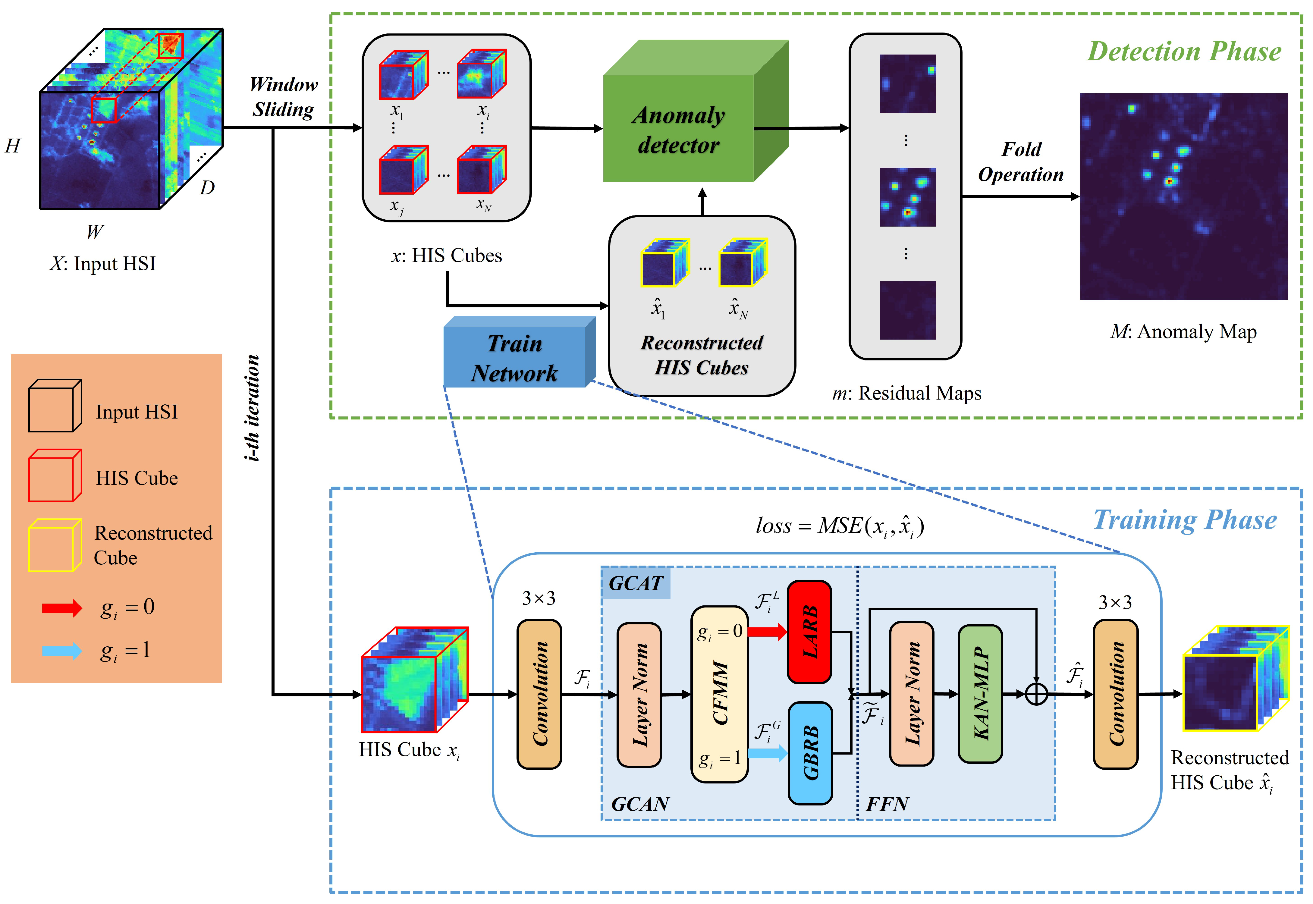
The KANGT framework operates in two phases, as shown in Figure 1. During the training phase, network optimization is achieved by minimizing reconstruction errors between input and output HSI cubes. Our architecture employs an efficient design philosophy, featuring a Fidelity-Gated Context-Aware Transformer core embedded between convolutional encoding and decoding layers. The GCAT module encompasses two complementary processing streams: the LARB and GBRB, which specialize in handling anomalous and background regions through distinct computational strategies. A dynamic gating mechanism, governed by our CFMM, determines the routing of feature maps between these branches.

Given an input HSI data volume $\mathcal{X}\in {\mathbb{R}}^{H\times W\times D}$ with spatial dimensions $H\times W$ and spectral bands D, we first decompose $\mathcal{X}$ into N overlapping cubes ${\left\{x_i\right\}}_{i=1}^N$ using a sliding window operation. The standard configuration employs $9\times 9$ spatial patches with a 3-pixel stride. These patches serve as training instances for network optimization.

The processing pipeline initiates with a convolutional encoder that transforms input cube $x_i$ into feature representation ${\mathcal{F}}_i\in {\mathbb{R}}^{H\times W\times C}$, where $C=64$ defines the feature dimensionality. The GCAT module then processes ${\mathcal{F}}_i$ to generate refined features ${\widehat{\mathcal{F}}}_i$, with branch selection controlled by gating signal $g_i$. Final reconstruction ${\widehat{x}}_i$ is produced through a convolutional decoder.

Network parameters $\mathrm{\Theta }$ are optimized by minimizing the reconstruction objective:

$$\mathcal{L}\left(\mathrm{\Theta }\right)={\displaystyle \frac{1}{B}}\sum _{i=1}^B{\parallel x_i-{\widehat{x}}_i\parallel }_F^2$$

(1)

where B denotes batch size and ${\parallel ·\parallel }_F$ represents the Frobenius norm [49].

During inference, anomaly scores are derived from residual tensors ${\mathcal{R}}_i={(x_i-{\widehat{x}}_i)}^2\in {\mathbb{R}}^{H\times W\times D}$, which are spatially aggregated and fused to produce the final detection map $\mathcal{M}\in {\mathbb{R}}^{H\times W}$. The proposed KANGT method is described in detail in Algorithm 1.

Algorithm 1 KANGT: Training and detection pipeline.

Require:  HSI data $\mathcal{X}$, patch size $h\times w$, stride $\sigma$, batch size B, max iterations $T_{\max }$, CFMM search period $T_s$. Ensure:  Anomaly map $\mathcal{M}$. Decompose $\mathcal{X}$ into N overlapping cubes ${\left\{x_i\right\}}_{i=1}^N$. Initialize parameters $\mathrm{\Theta }$, gating states $\Gamma ={\left\{g_i\right\}}_{i=1}^N\leftarrow \mathbf{0}$. {Training Phase} for iteration $t=1$ to $T_{\max }$ do    Sample mini-batch ${\left\{x_i\right\}}_{i=1}^B$ from ${\left\{x_i\right\}}_{i=1}^N$.    for each $x_i$ in the batch do      ${\mathcal{F}}_i\leftarrow \mathrm{Encoder}\left(x_i\right)$      ${\tilde{\mathcal{F}}}_i\leftarrow \mathrm{GCAN}({\mathcal{F}}_i,g_i)$ (using Equation (2))      ${\widehat{\mathcal{F}}}_i\leftarrow \mathrm{Dropout}\left(\mathrm{KAN}\_\mathrm{Layer}\left(\mathrm{LN}\left({\tilde{\mathcal{F}}}_i\right)\right)\right)+{\tilde{\mathcal{F}}}_i$ (using Equation (5))      ${\widehat{x}}_i\leftarrow \mathrm{Decoder}\left({\widehat{\mathcal{F}}}_i\right)$    end for    Compute loss $\mathcal{L}\left(\mathrm{\Theta }\right)={\displaystyle \frac{1}{B}}{\sum }_{i=1}^B{\parallel x_i-{\widehat{x}}_i\parallel }_F^2$ (Equation (1)).    Update $\mathrm{\Theta }$ via gradient descent.    if $tmod{T}_s=0$ and $t\ne T_{\max }$ then      Update $\mathrm{\Gamma }$ via CFMM (Section 3.3, Equations (11)–(13)).    end if end for {Detection Phase} Initialize empty list ${\mathcal{S}}_{\mathrm{list}}$ for each cube $x_i$ in ${\left\{x_i\right\}}_{i=1}^N$ do    Generate reconstruction ${\widehat{x}}_i$ using trained model $\mathrm{\Theta }$.    Compute 3D residual ${\mathcal{R}}_i={(x_i-{\widehat{x}}_i)}^2$.    Apply multi-scale diffusion ${\mathcal{E}}_i\leftarrow \mathrm{MultiScalePool}\left({\mathcal{R}}_i\right)$ (Equation (14)).    Aggregate 2D score ${\mathcal{S}}_i={\sum }_{d=1}^D{\mathcal{E}}_i^{\left(d\right)}$ (Equation (15)).    Append ${\mathcal{S}}_i$ to ${\mathcal{S}}_{\mathrm{list}}$. end for Fuse final map $\mathcal{M}\leftarrow \Psi \left({\mathcal{S}}_{\mathrm{list}}\right)$ (Equation (16)). return $\mathcal{M}$

3.2. Fidelity-Gated Context-Aware Transformer Architecture

The GCAT module forms the computational core of our framework, structured as a sequential composition of a gated context-aware network (GCAN) and KAN-enhanced FFN. The GCAN implements conditional feature processing through dual specialized branches, while the FFN performs non-linear feature enhancement.

3.2.1. Gated Context-Aware Network

The GCAN employs a switching mechanism that directs input features through appropriate processing pathways based on content characteristics. For input feature tensor ${\mathcal{F}}_i$, the gating controller generates a binary decision signal $g_i$ that selects between LARB and GBRB processing:

$${\tilde{\mathcal{F}}}_i=\left\{\begin{array}{cc}{\mathcal{H}}_{\mathrm{LARB}}\left(\mathrm{LN}\left({\mathcal{F}}_i\right)\right),\hfill & \mathrm{if}{g}_i=0\hfill \\ {\mathcal{H}}_{\mathrm{GBRB}}\left(\mathrm{LN}\left({\mathcal{F}}_i\right)\right),\hfill & \mathrm{if}{g}_i=1\hfill \end{array}\right.$$

(2)

where ${\mathcal{H}}_{\mathrm{LARB}}$ and ${\mathcal{H}}_{\mathrm{GBRB}}$ represent the transformation functions of the respective branches and LN denotes layer normalization.

3.2.2. KAN-Enhanced Feature Transformation

Traditional FFNs within Transformer architectures rely on fixed non-linear activation functions (e.g., ReLU or GELU) interleaved with linear projections. This design fundamentally limits the model’s ability to approximate the highly non-linear and continuous spectral signatures inherent in HSI data, as the network is constrained to approximate complex spectral curves using piecewise linear functions. To overcome this limitation and enhance the representation capacity of the GCAT, we introduce the KAN-MLP module, which replaces fixed node-based activations with learnable edge-based activations grounded in the Kolmogorov–Arnold representation theorem.

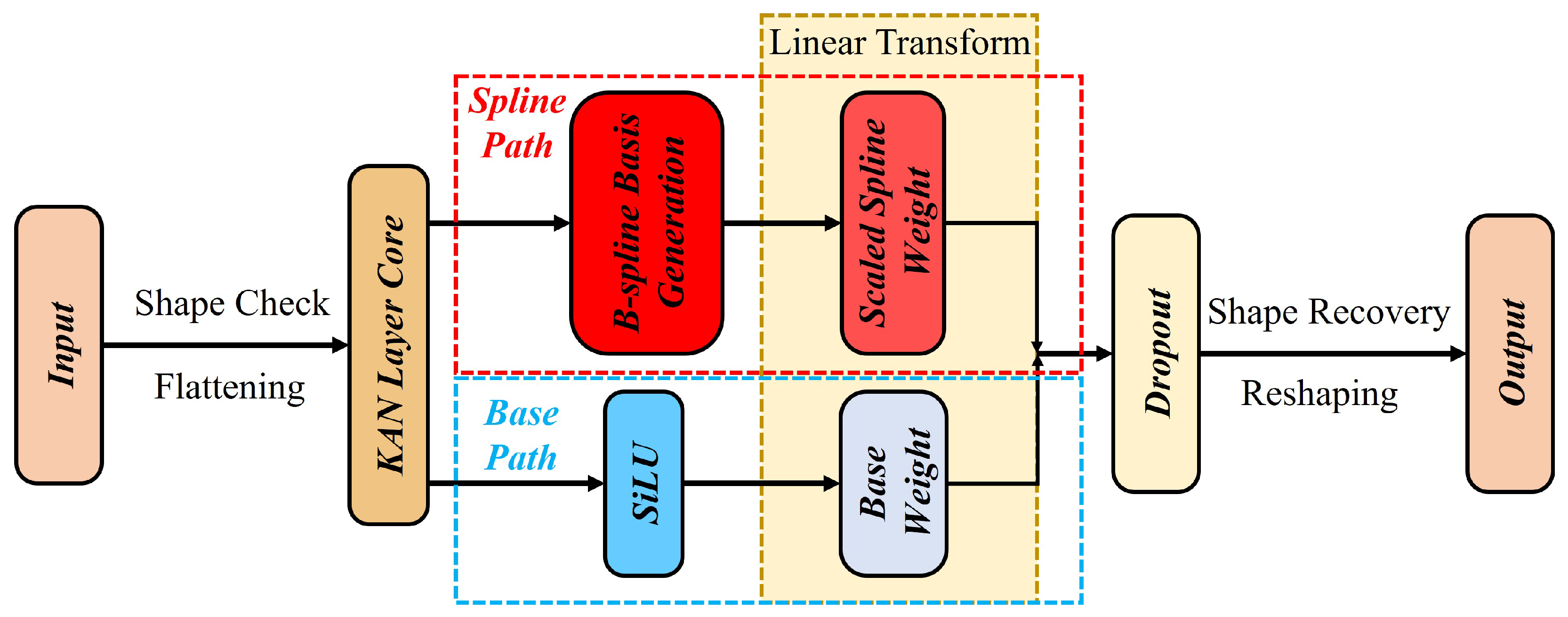
The KAN-MLP module employs a dual-path architecture designed to balance representational plasticity with optimization stability. As illustrated in Figure 2, for an input feature tensor $\mathcal{X}\in {\mathbb{R}}^{N\times C}$, the transformation is decomposed into two parallel processing branches: a base regularization pathand a spline reconstruction path.

The output feature $\mathcal{Z}$ of a KAN layer is formulated as the additive fusion of these two paths:

$$\mathcal{Z}=\underset{\mathrm{Base}\mathrm{Path}}{\underbrace{\sigma \left(\mathcal{X}\right){\mathbf{W}}_b}}+\underset{\mathrm{Spline}\mathrm{Path}}{\underbrace{{\mathrm{\Phi }}_s\left(\mathcal{X}\right){\mathbf{W}}_s}}$$

(3)

where ${\mathbf{W}}_b$ and ${\mathbf{W}}_s$ denote the learnable weight matrices for the base and spline paths, respectively.

(1)

Base Regularization Path:

The first branch captures the global, low-frequency non-linear trends of the data and acts as a structural prior. It utilizes the Sigmoid Linear Unit (SiLU) as the activation function $\sigma (·)$, defined as $\sigma \left(x\right)=x·\mathrm{sigmoid}\left(x\right)$. We strictly select SiLU over the conventional ReLU for two theoretical reasons essential to the KAN architecture:

• ${\mathcal{C}}^{\infty }$ Continuity: Unlike the piecewise-linear ReLU, which is non-differentiable at zero (${\mathcal{C}}^0$), SiLU is smooth and continuously differentiable (${\mathcal{C}}^{\infty }$). This matches the curvature continuity of the cubic B-splines used in the second path, ensuring a consistent gradient field during backpropagation and preventing optimization instability caused by discontinuous derivatives.
• Gradient Preservation: In anomaly detection, normalized spectral residuals often center around zero. SiLU’s non-monotonic property and linear approximation near the origin ($\sigma \left(x\right)\approx x$) allow the base path to effectively act as a linear residual connection for small signals. This preserves gradient flow through deep layers and mitigates the “dying ReLU” problem where negative spectral deviations—crucial for identifying absorption features—are zeroed out.

(2)

Spline Reconstruction Path: The second branch models the fine-grained, high-frequency spectral details (such as subtle anomaly absorption features). It employs a linear combination of B-spline basis functions. The spline transformation ${\mathrm{\Phi }}_s\left(\mathcal{X}\right)$ expands each scalar input x into a set of basis responses:

$$\mathrm{spline}\left(x\right)=\sum _{i=0}^{G+k-1}{c}_i{B}_i\left(x\right)$$

(4)

where $B_i\left(x\right)$ represents the i-th B-spline basis function of order $k=3$ (cubic) defined on a grid of size $G=5$, and $c_i$ are the learnable control coefficients implicitly contained within ${\mathbf{W}}_s$. This formulation enables the network to learn a custom, non-monotonic activation shape for every spectral feature dimension, effectively creating an adaptive spectral index.

(3)

Integration and Weighting: The outputs of the two paths are fused via element-wise addition, as shown in Equation (3). This additive coupling allows the network to automatically weight the contribution of each path during training: the matrix ${\mathbf{W}}_b$ learns the coarse structural relationships, while ${\mathbf{W}}_s$ refines the feature space by capturing complex non-linear deviations. Finally, the complete KAN-MLP block within the Transformer is defined as follows:

$${\widehat{\mathcal{F}}}_i=\mathrm{Dropout}(\mathrm{KAN}\text{\_}\mathrm{Layer}(\mathrm{LN}({\tilde{\mathcal{F}}}_i)))+{\tilde{\mathcal{F}}}_i$$

(5)

where $\mathrm{KAN}\text{\_}\mathrm{Layer}(·)$ represents the dual-path operations described above and LN denotes layer normalization.

3.2.3. Local Anomaly Recognition Branch

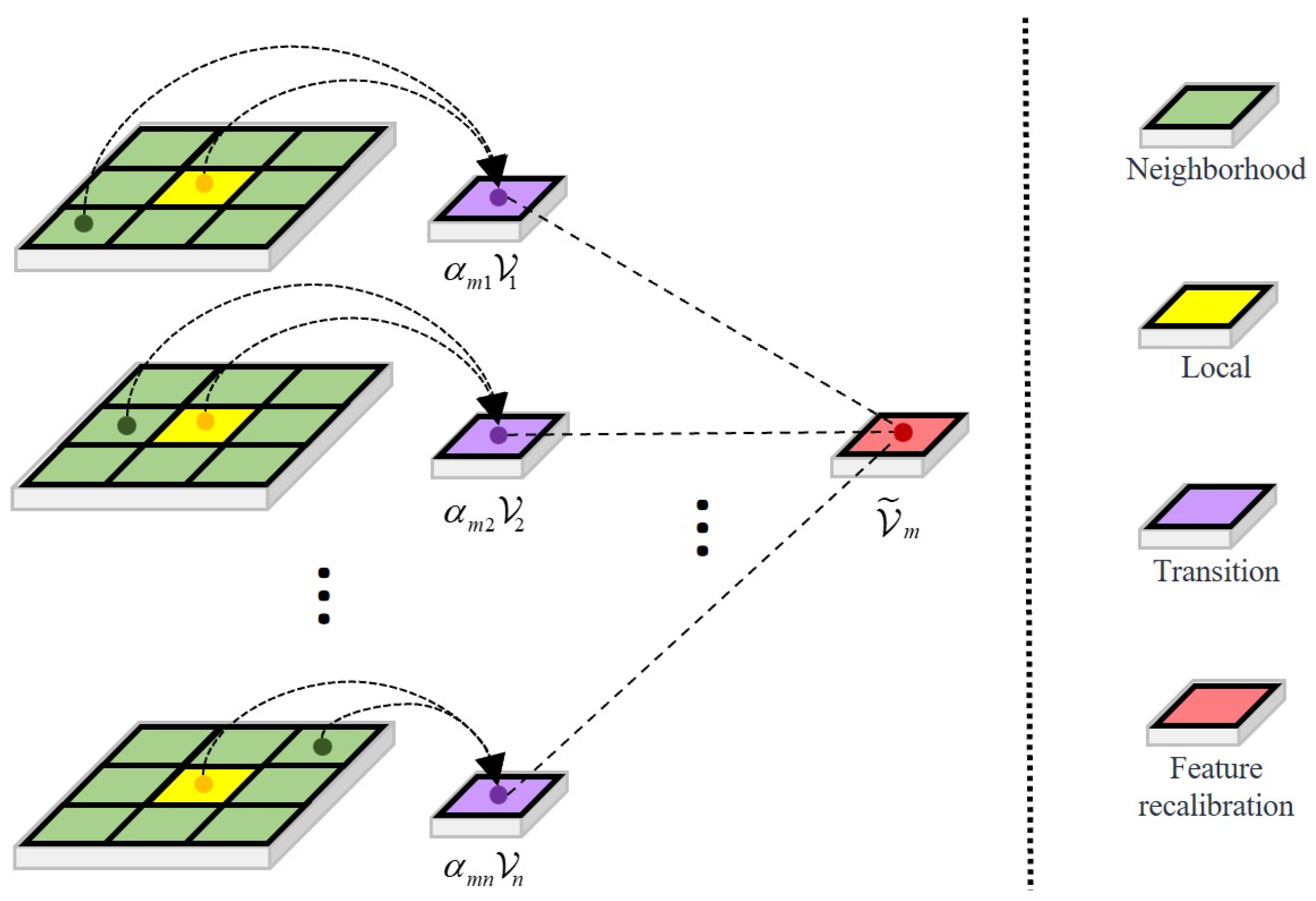
The LARB targets anomalous region suppression through local context analysis and feature recalibration. Input features ${\mathcal{F}}_i^L$ are decomposed into $K_L$ non-overlapping patches ${\left\{{\mathcal{V}}_k\right\}}_{k=1}^{K_L}$ of dimension $M_L\times C$, with $M_L=3\times 3$.

Inter-patch affinity computation employs learned projections:

$$A({\mathcal{V}}_m,{\mathcal{V}}_n)=\left({\mathcal{V}}_m{\mathbf{W}}_L\right){\left({\mathcal{V}}_n{\mathbf{W}}_L\right)}^{\top }$$

(6)

where ${\mathbf{W}}_L\in {\mathbb{R}}^{C\times C/4}$ implements dimensional reduction.

Normalized attention weights are obtained through the softmax operation:

$${\alpha }_{mn}={\displaystyle \frac{exp(A({\mathcal{V}}_m,{\mathcal{V}}_n)/\tau )}{{\sum }_{j\in {\mathcal{N}}_m}exp(A({\mathcal{V}}_m,{\mathcal{V}}_j)/\tau )}}$$

(7)

where ${\mathcal{N}}_m$ denotes neighborhood indices and $\tau$ is the selectivity parameter that governs the concentration of the normalized attention weights, effectively adjusting the trade-off between local averaging and sharp feature focusing.

Feature recalibration aggregates contextual information:

$${\tilde{\mathcal{V}}}_m=\sum _{n\in {\mathcal{N}}_m}{\alpha }_{mn}{\mathcal{V}}_n$$

(8)

The output tensor ${\tilde{\mathcal{F}}}_i$ is reconstructed by reassembling recalibrated patches. The process of the LARB is shown in Figure 3.

3.2.4. Global Background Recognition Branch

The GBRB enhances background representation through global attention mechanisms. Input ${\mathcal{F}}_i^G$ is partitioned into $K_G$ patches and reshaped to ${\mathcal{T}}_G\in {\mathbb{R}}^{K_G\times M_G\times C}$.

The self-attention computation employs shared projections:

$$\mathcal{Q}={\mathcal{T}}_G{\mathbf{W}}_G,\mathcal{K}={\mathcal{T}}_G{\mathbf{W}}_G,\mathcal{V}={\mathcal{T}}_G$$

(9)

$${\tilde{\mathcal{F}}}_i=\mathrm{Reshape}\left(\mathrm{Softmax}\right(\mathcal{Q}{\mathcal{K}}^{\top }\left)\mathcal{V}\right)$$

(10)

where ${\mathbf{W}}_G$ shares parameters with ${\mathbf{W}}_L$ to maintain consistency.

3.3. Contextual Feature Matching Module

The CFMM is a core innovation of KANGT, designed to explicitly address the “uniform processing” limitation inherent in standard Transformer architectures. Its function is to dynamically route input cubes to the branch best suited for their content (background or anomaly) based on an interpretable, data-driven measure of reconstruction fidelity.

Unlike other gated architectures that may rely on learned soft-attention weights or implicit “adaptive gating units,” the CFMM provides an explicit, fidelity-based routing decision. The module operates on the central hypothesis of reconstruction-based HAD: background patches, which constitute the majority of the data, can be reconstructed by the network with high fidelity, whereas anomalous patches, due to their statistical rarity, cannot. The CFMM leverages this disparity to segregate the data streams.

The gating mechanism is not static; it is updated iteratively throughout the training process, as detailed in Algorithm 1. Initially, all gating states in $\mathrm{\Gamma }={\left\{g_i\right\}}_{i=1}^N$ are initialized to zero ($g_i=0$), forcing all input cubes through the LARB. This allows the network to first learn a general-purpose representation focused on suppressing hard-to-reconstruct (potentially anomalous) features.

At periodic intervals (e.g., every $T_s$ iterations), the CFMM re-evaluates the gating state for each training cube $x_i$. This evaluation is a direct assessment of reconstruction fidelity. For a given reconstructed cube ${\widehat{x}}_i$, the module computes its Euclidean distance to all original cubes ${\left\{x_j\right\}}_{j=1}^N$ in the dataset (or a representative subset):

$$\delta ({\widehat{x}}_i,x_j)={\parallel {\widehat{x}}_i-x_j\parallel }_2$$

(11)

The module then identifies the index $\nu$ of the nearest neighbor (i.e., the most similar original cube) to the reconstruction ${\widehat{x}}_i$:

$$\nu =\underset{j}{argmin}\delta ({\widehat{x}}_i,x_j)$$

(12)

The gating signal $g_i$ is then updated based on a strict fidelity criterion. The gate $g_i$ is set to 1 (route to the GBRB) if and only if the reconstruction ${\widehat{x}}_i$ is closer to its own original input $x_i$ than to any other original cube $x_j$. This indicates that the model has successfully and uniquely identified its background pattern.

$$g_i\leftarrow \mathbb{I}[\nu =i]$$

(13)

where $\mathbb{I}[·]$ is the indicator function. A gate value of $g_i=1$ signifies high reconstruction fidelity (assumed background), routing the cube to the GBRB. Conversely, a value of $g_i=0$ signifies low fidelity (a potential anomaly or highly complex/unique background patch), retaining the cube in the LARB.

This dynamic interaction between the CFMM and the GCAT dual branches creates the “self-improving loop” that is central to our design. As training progresses, the model’s reconstruction quality for background patches improves. The CFMM identifies these high-fidelity cubes and progressively redirects them to the GBRB. This action allows the GBRB to specialize its parameters for modeling a pure, global background. Concurrently, this specialization purges the LARB of simple background patches, enabling it to focus its representational power exclusively on suppressing the reconstruction of challenging, low-fidelity anomalous regions. This explicit, fidelity-based specialization is the key mechanism by which KANGT separates the background and anomaly representations. The specific CMM procedure is illustrated in Figure 4.

3.4. Anomaly Detection and Residual Enhancement

The anomaly detection process is initiated by analyzing the reconstruction residuals, which capture the pixel-wise squared error between the input cube $x_i$ and its reconstruction ${\widehat{x}}_i$. This yields an initial 3D residual tensor ${\mathcal{R}}_i={(x_i-{\widehat{x}}_i)}^2$.

To mitigate boundary artifacts and enhance detection sensitivity, we first employ a multi-scale residual diffusion strategy on this 3D tensor. This enhanced residual ${\mathcal{E}}_i$ is computed by averaging 3D average-pooled features across multiple spatial and spectral scales, which improves anomaly localization while suppressing false alarms in homogeneous regions:

$${\mathcal{E}}_i={\displaystyle \frac{1}{3}}\sum _{s\in \{3,5,7\}}{\mathrm{AvgPool}3\mathrm{d}}_{s\times s\times 5}\left({\mathcal{R}}_i\right)$$

(14)

Following this 3D enhancement, spectral aggregation is performed on the diffused residual tensor ${\mathcal{E}}_i$ to collapse the spectral dimension and produce 2D anomaly scores ${\mathcal{S}}_i$:

$${\mathcal{S}}_i=\sum _{d=1}^D{\mathcal{E}}_i^{\left(d\right)}$$

(15)

Finally, the composite anomaly map $\mathcal{M}$ is generated through the spatial fusion of all overlapping 2D score patches derived from the entire HSI cube:

$$\mathcal{M}=\Psi \left({\left\{{\mathcal{S}}_i\right\}}_{i=1}^N\right)$$

(16)

where $\Psi$ implements an overlapping region averaging strategy to produce the final, coherent detection map.

4. Results

This section contrasts KANGT’s performance against eight established HAD techniques across eight real HSI datasets, demonstrating significant superiority.

4.1. Dataset Description

Here we introduce the eight HSI datasets.

• The AVIRIS sensor’s latest dataset, the seventh in the series, captures the L.A. landscape. The image measures 100 by 100 in spatial dimensions, boasting a 7.1 m pixel resolution. After some noise filtering, we are left with 205 spectral bands. This dataset puts the spotlight on artificial structures nestled within nature, featuring 28 rogue pixels that make up just 0.36% of the total pixel count.
• The second installment in our collection comes from the Cat Island region, captured with impressive detail at 17.2 m per pixel across a 120 by 120 pixel grid. After weeding out the unreliable spectral bands, we are left with 188 solid bands for our analysis. The dataset contains just one anomaly—a lone airplane represented by 19 rogue pixels, making up a mere 0.13% of the total pixel count. Following in the footsteps of the other datasets, the AVIRIS sensor was the tool of choice for gathering this information.
• The Gulfport dataset, our third entry, was captured via the AVIRIS sensor. The Los Angeles-2 dataset boasts a spatial resolution of 3.4 m per pixel. Once filtered for quality, the image spans a 100 by 100 spatial area and includes 191 distinct spectral bands. The anomalies detected originated from three planes of varying sizes, totalling 60 pixel anomalies. That may not sound like much, but it does account for 0.60% of the total pixel count.
• The Los Angeles-1 dataset was assembled utilizing state-of-the-art AVIRIS sensor tech, capturing aerial visuals of the City of Angels. The dataset boasts a 100 by 100 pixel grid, with each pixel offering a spatial clarity of 7.1 m. This impressive detail is captured across a spectrum of 205 different color bands. What is more, there are 144 pixels that stick out like a sore thumb, presumably from different aircraft. These rogue pixels account for a mere 1.44% of the entire pixel population.
• The AVIRIS sensor in Los Angeles has assembled another dataset for us. Los Angeles-2 features two planes, each with 87 pixels that are out of the ordinary—these make up just 0.87% of the entire image’s pixel count. The dataset comprises 205 spectral bands, spans 100 × 100 in size, and boasts a nifty spatial resolution of 7.1 m per pixel.
• The Pavia dataset, our sixth set of data, was captured with the help of the Reflective Optics System Imaging Spectrometer, or ROSIS, for short. The imagery spans 150 pixels by 150 pixels, boasting a spatial resolution of 1.3 m per pixel. It also features 102 spectral bands, with some less than ideal ones having been omitted. The main quirks in this dataset are a handful of vehicles parked on the bridge, totaling 68 pixels that stand out, accounting for just 0.30% of the overall pixel count.
• The San Diego dataset, which represents the final acquisition from the AVIRIS sensor, features two authentic hyperspectral scenes. This collection encompasses 189 spectral bands across a 100 × 100 pixel grid, offering a spatial resolution of 7.5 m per pixel. The primary backdrop consists of structures like hangars and aprons alongside soil, while three aircraft serve as the anomalies, distributed across 134 pixels and comprising 1.34% of the total image area.
• The last installment of the Texas Coast dataset was gathered using the AVIRIS sensor, which produced a 100 × 100 pixel grid with each pixel covering 17.2 m of space. This comprehensive dataset spans 204 spectral bands and contains a number of houses with atypical characteristics, specifically 67 anomalous pixels that make up 0.67% of the total pixel count.

4.2. Compared Methods and Parameter Settings

Eight advanced methods were chosen for evaluating the detection performance of the developed KANGT method in the experiments. These methods are RX [6], 2S-GLRT [50], MsRFQFT [51], PCA-TLRSR [9], GT-HAD [52], LREN [53], Auto-AD [11], and DFAN [54]. RX, 2S-GLRT, and MsRFQFT belong to statistics-based techniques, while PCA-TLRSR is a representation-based approach. On the other hand, LREN, Auto-AD, and DFAN are DNN-based methods. The aforementioned methods represent either classical or cutting-edge algorithms for hyperspectral anomaly detection, each demonstrating remarkable performance in identifying anomalous targets. Subsequently, anomaly detection will be conducted on the previously mentioned datasets by integrating the optimal parameters recommended by the respective authors in their publications with those determined through practical experimentation. As shown in

Table 1. Parameter values for the compared methods on the first 4 datasets.

Methods	Parameters	Los Angeles-1	Los Angeles-2	Gulfport	Texas Coast
RX	/	/	/	/	/
2S-GLRT	$(w_{\mathrm{in}},w_{\mathrm{out}})$	(7, 9)	(15, 19)	(11, 13)	(5, 9)
MsRFQFT	$(N_d,\sigma )$	(3, 1.2)	(3, 4.0)	(3, 10)	(3, 1.4)
GT-HAD	/	/	/	/	/
PCA-TLRSR	$(d,\lambda ,{\lambda }^{\prime })$	(4, 0.06, 0.01)	(5, 0.06, 0.01)	(17, 0.06, 0.05)	(15, 0.06, 0.02)
Auto-AD	$\sigma$	$1.0\times {10}^{-5}$	$1.5\times {10}^{-5}$	$1.2\times {10}^{-5}$	$1.0\times {10}^{-5}$
LREN	$\lambda$	1.0	0.1	0.001	1.0
DFAN	(MinPts, Eps, Epochs, LR)	(6, 0.5, 20, 0.01)	(3, 0.3, 10, 0.0001)	(2, 0.5, 20, 0.0001)	(4, 0.5, 20, 0.0001)
KANGT	KAN grid size	10	7	5	5

and

Table 2. Parameter values for the compared methods on the last 4 datasets.

Methods	Parameters	Cat Island	Pavia	ABU-Urban-4	San Diego
RX	/	/	/	/	/
2S-GLRT	$(w_{\mathrm{in}},w_{\mathrm{out}})$	(3, 25)	(5, 21)	(11, 13)	(5, 25)
MsRFQFT	$(N_d,\sigma )$	(3, 0.4)	(3, 1.6)	(3, 1.7)	(3, 6.3)
GT-HAD	/	/	/	/	/
PCA-TLRSR	$(d,\lambda ,{\lambda }^{\prime })$	(15, 0.06, 0.02)	(4, 0.05, 0.01)	(5, 0.06, 0.01)	(5, 0.05, 0.01)
Auto-AD	$\sigma$	$1.0\times {10}^{-5}$	$1.0\times {10}^{-5}$	$1.0\times {10}^{-5}$	$1.0\times {10}^{-5}$
LREN	$\lambda$	1.0	1.0	0.0001	0.01
DFAN	(MinPts, Eps, Epochs, LR)	(2, 0.5, 20, 0.01)	(6, 0.6, 20, 0.0001)	(6, 0.5, 20, 0.01)	(6, 0.5, 20, 0.01)
KANGT	KAN grid size	5	5	5	3

, we give the parameter values of all compared algorithms and the KAN grid size of KANGT for each dataset.

The proposed KANGT was computed using an NVIDIA GeForce RTX 3060 GPU and Intel i7 processors, implemented within the PyTorch framework on the Windows 11 operating system. The model underwent training leveraging the adaptive moment estimation (ADAM) optimizer, with the following hyperparameter settings: the entire training regimen spanned 150 epochs, processing data in batches of 64, while maintaining a learning rate set at 0.001. Additionally, KANGT, DFAN, and Auto-AD utilize PyTorch 2.2.0, whereas LREN employs TensorFlow 1.14.0. In contrast, all non-DNN methods are implemented in MATLAB 2022a.

4.3. Detection Performance

Our study uses a blend of quality and quantity metrics to gauge the effectiveness of various HAD methodologies. Qualitative assessments include the anomaly heatmap [5], the box–whisker plot [55], the 2-D ROC curves [56], and a quantitative measure through the Area Under the Curve (AUC) calculation. This multi-faceted evaluation considers various angles to measure the efficiency of anomaly detection. The heatmap provides a visual representation of background suppression and anomaly detection performance, while the box-and-whisker plot evaluates how clearly the system can differentiate between normal and anomalous data. The effectiveness of an HAD approach becomes evident through a 2-D ROC curve situated in the upper-left region and an elevated AUC value, which indicates a reduced number of false alarms. A perfect AUC score of 1 signifies the optimal outcome where every anomaly is correctly identified without any mistakes.

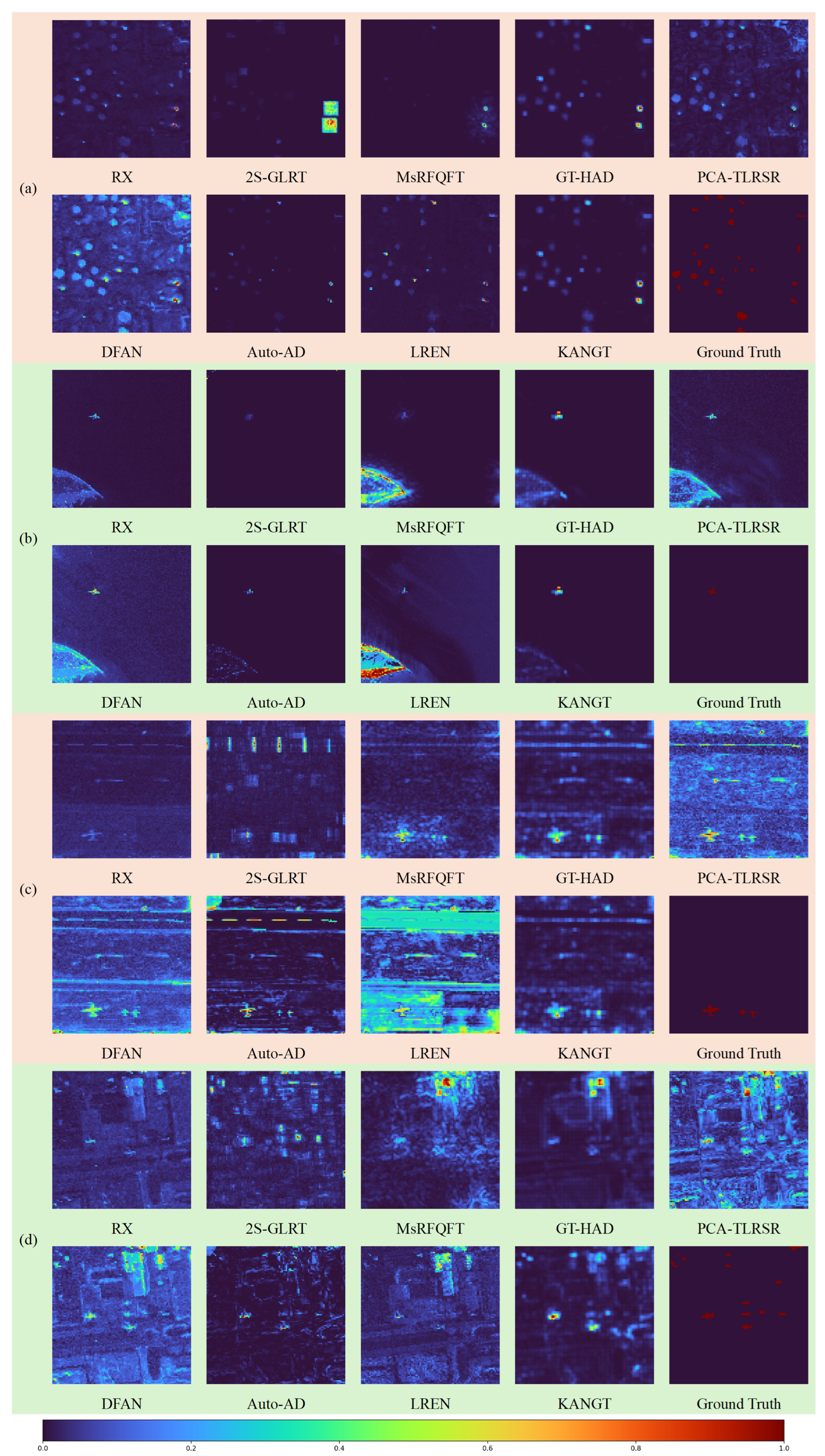
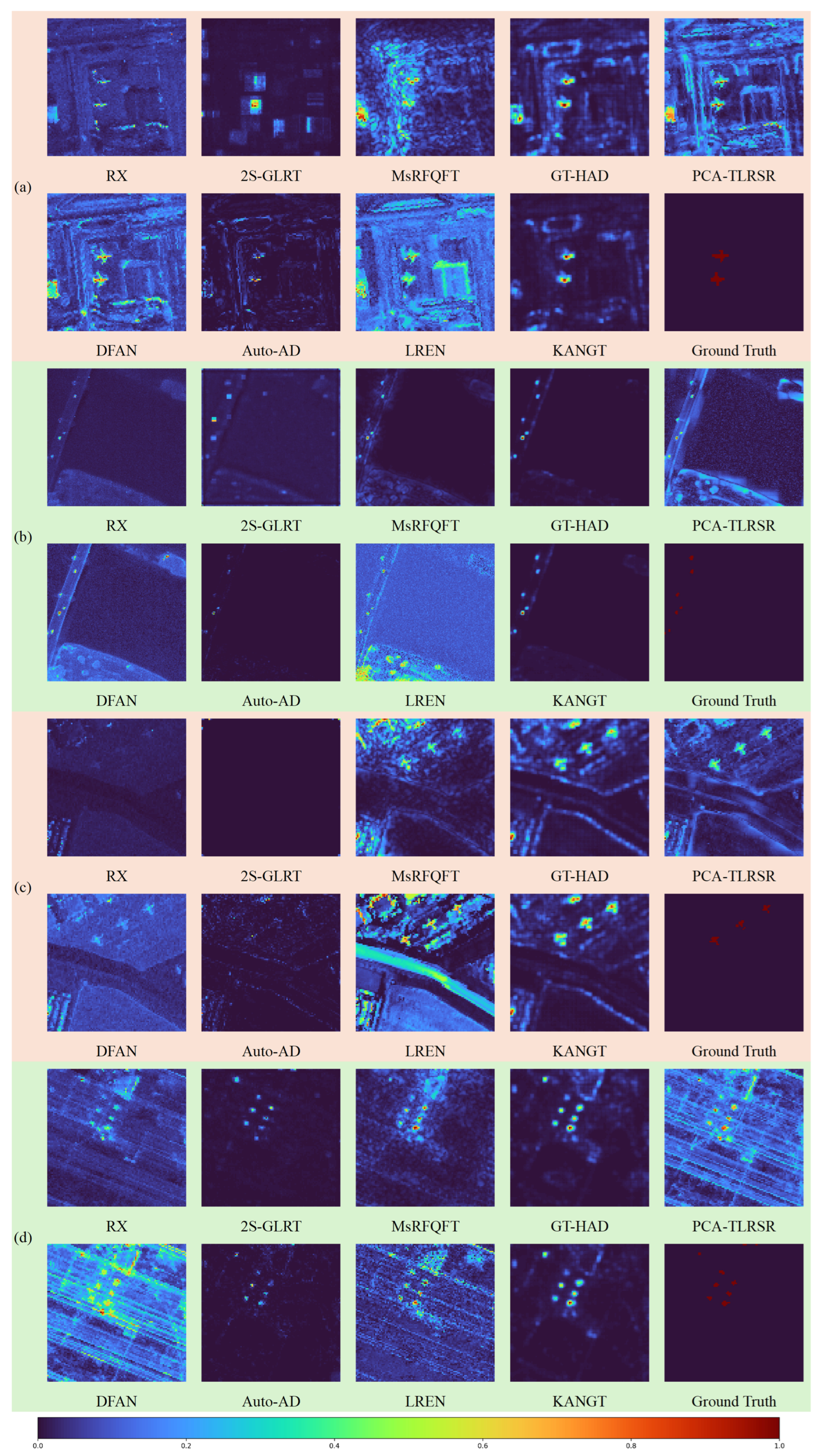
Figure 5 and Figure 6 present the anomaly heatmaps of different methods on each dataset. The experimental results demonstrate that KANGT effectively balances background suppression and anomaly response on several datasets, namely ABU-urban-4, Gulfport, Los Angeles-1, Los Angeles-2, and Pavia. Taking the San Diego dataset as a specific case, while RX, 2S-GLRT, PCA-TLRSR, and Auto-AD demonstrate a high degree of background suppression, they either fail to identify the requisite anomalous targets or exhibit insufficient sensitivity in detecting them. Conversely, methods like LREN and MsRFQFT are more capable of highlighting anomalies, yet they introduce a significant number of false alarms within the background clutter. Furthermore, KANGT demonstrates superior background suppression capability compared to DFAN and LREN. Among the nine methods evaluated on the eight datasets, only PCA-TLRSR on the ABU-urban-4 dataset and Auto-AD on the San Diego dataset demonstrate performance that is comparable to that of KANGT. These anomaly heatmaps collectively present some pretty striking visual proof that KANGT has managed achieve remarkable results: it effectively reconstructs the background, all while keeping those pesky anomalies in check.

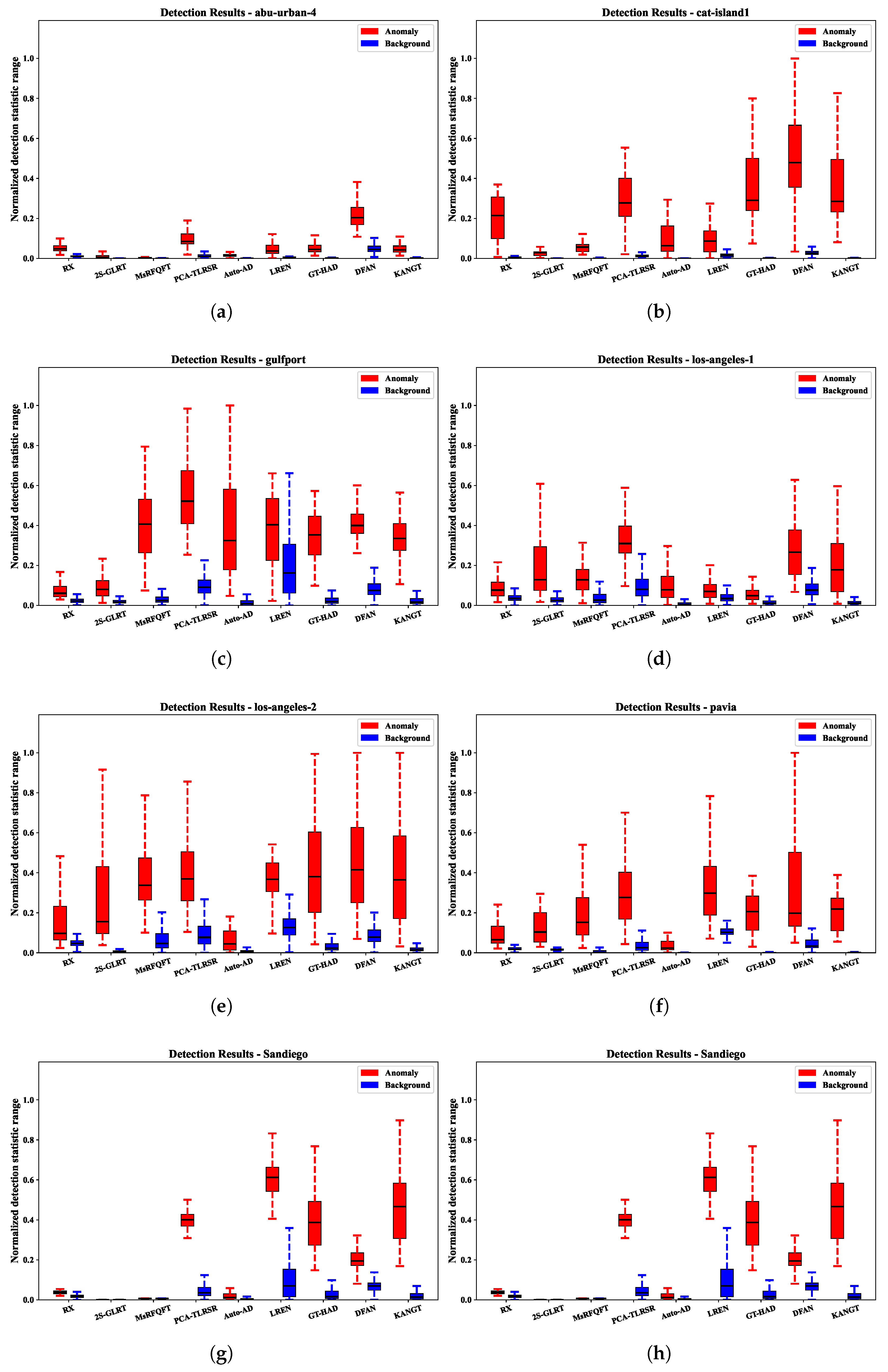
Figure 7 presents the box-and-whisker plots generated by the nine methods on the eight datasets. These plots illustrate the distribution of abnormal pixels (within the crimson boxes) and background pixels (within the azure boxes). The distinction between the red and blue squares reveals the degree of distinction between the backdrop and irregularities. Specifically, the height of the azure box indicates the efficiency of background elimination. As shown in Figure 7, KANGT achieves a harmonious balance between background–anomaly separateness and background elimination across all eight datasets. For instance, although GT-HAD performs very well on most datasets and can better separate the background from anomalies, it generates a large number of false alarms on the Los Angeles-1 dataset. Conversely, 2S-GLRT excels in background elimination but struggles in distinguishing the background from anomalies. In contrast, KANGT performs well in both aspects. In conclusion, the capability of KANGT to enhance background reconstruction while suppressing anomaly reconstruction contributes to its satisfactory performance.

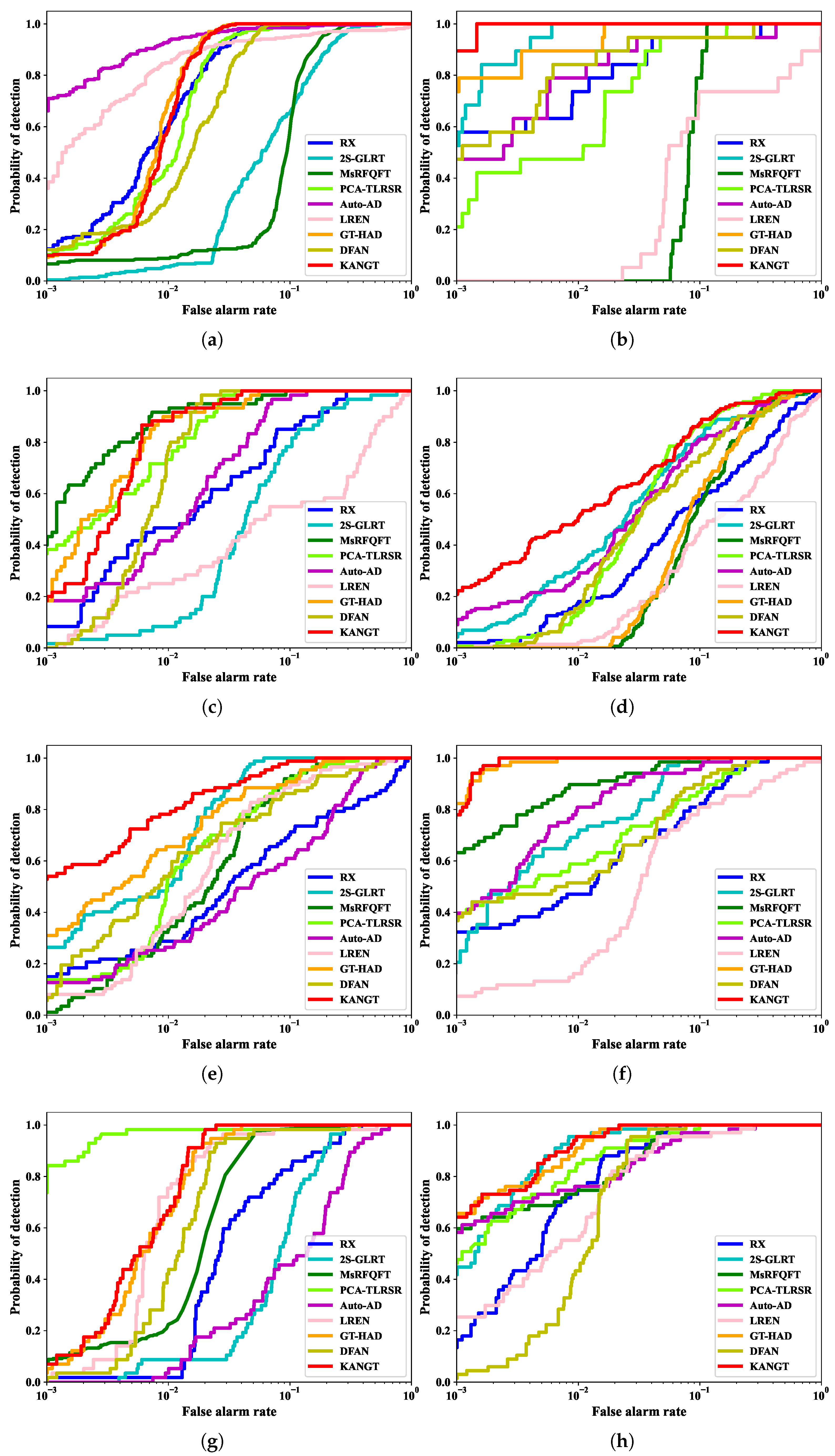
Figure 8 illustrates the 2-D curves for the nine methods across the eight datasets. Visual inspection reveals that KANGT’s 2-D ROC curve consistently lies closest to the desirable upper left corner in the majority of scenes. An in-depth analysis of the Los Angeles-2 dataset reveals that while 2S-GLRT marginally edges out its competitors in terms of detection success during the false-alarm window of 0.05 to 0.1, KANGT maintains superior performance overall, with its results consistently aligning more closely with the ideal standard. This quantitative superiority is corroborated by the AUC scores in

Table 3. Performance comparison of hyperspectral anomaly detection methods (AUC scores).

Dataset	KANGT	RX	2S-GLRT	MsRFQFT	GT-HAD	PCA-TLRSR	Auto-AD	LREN	DFAN
ABU-Urban-4	0.9906	0.9887	0.9099	0.9762	0.9912	0.9865	0.9942	0.9687	0.9811
Cat Island	0.9994	0.9764	0.9985	0.9976	0.9793	0.9793	0.9732	0.7647	0.9817
Gulfport	0.9945	0.9526	0.9183	0.9945	0.9937	0.9931	0.9768	0.7774	0.9919
Los Angeles-1	0.9740	0.8221	0.9236	0.8688	0.8711	0.9455	0.9211	0.7461	0.9139
Los Angeles-2	0.9893	0.8404	0.9873	0.9634	0.9762	0.9664	0.8784	0.9505	0.9459
Pavia	0.9995	0.9538	0.9868	0.9943	0.9994	0.9636	0.9886	0.8976	0.9664
San Diego	0.9923	0.9398	0.9035	0.9715	0.9910	0.9928	0.8406	0.9814	0.9812
Texas Coast	0.9976	0.9907	0.9970	0.9911	0.9974	0.9925	0.9846	0.9810	0.9864
Average	0.9921	0.9328	0.9642	0.9490	0.9772	0.9975	0.9459	0.8835	0.9684

Bold values indicate the best performance on each dataset.

, where KANGT attains the top score on six datasets for which AUC is calculated, with its performance on the remaining two also ranking highly. The 3-D ROC curves further demonstrate KANGT’s robust capability to maintain an effective PD-FAR trade-off across all thresholds and datasets. Collectively, these findings validate both the stability of KANGT across various scenarios and its consistent high performance under different operational settings.

To situate the performance of KANGT within the landscape of existing dual-branch architectures, a direct comparison with DFAN [54] is undertaken. As shown in Figure 3, although DFAN has achieved notable success across multiple datasets through feature aggregation (with an average AUC of 0.9684), its performance markedly deteriorates when confronted with the highly complex Los Angeles-1 dataset, where it achieves an AUC of only 0.9139. In contrast, KANGT attains an AUC of 0.9740 on the same dataset, marking a statistically significant improvement of 6.01% over DFAN. This pronounced disparity in performance powerfully attests to the advantages of fidelity-gated routing. In intricate scenarios, the precise "filtering" of anomalies from a convoluted array of background textures is contingent upon explicit routing underpinned by physical metrics, a process essential for ensuring detection robustness. Collectively, KANGT establishes a new state of the art with an average AUC of 0.9921, outperforming the aggregation-based DFAN (0.9684) by a margin of 2.4 percentage points, thus substantiating the paradigm shift from "fusion" to "isolation" in architectural design. A comparative analysis with recent state-of-the-art algorithms, including KACNet [21] and HTC-HAD [15], reveals that the KANGT algorithm attains an AUC score of 0.9923 on the San Diego dataset. This represents a marginal increase over KACNet’s score of 0.9915 and is broadly equivalent to the performance of HTC-HAD on the same dataset (AUC = 0.9922). Similarly, on the ABU-Urban-4 dataset, the KANGT algorithm yields an AUC value of 0.9906, exhibiting a performance comparable to that of the KACNet algorithm (AUC = 0.9932). Most significantly, in contrast to the AUC score of 0.9932 achieved by the GTC-HAD algorithm on the Pavia dataset, the KANGT algorithm demonstrates a marked enhancement, achieving an AUC of 0.9995, approaching a perfect level.

4.4. Ablation Study

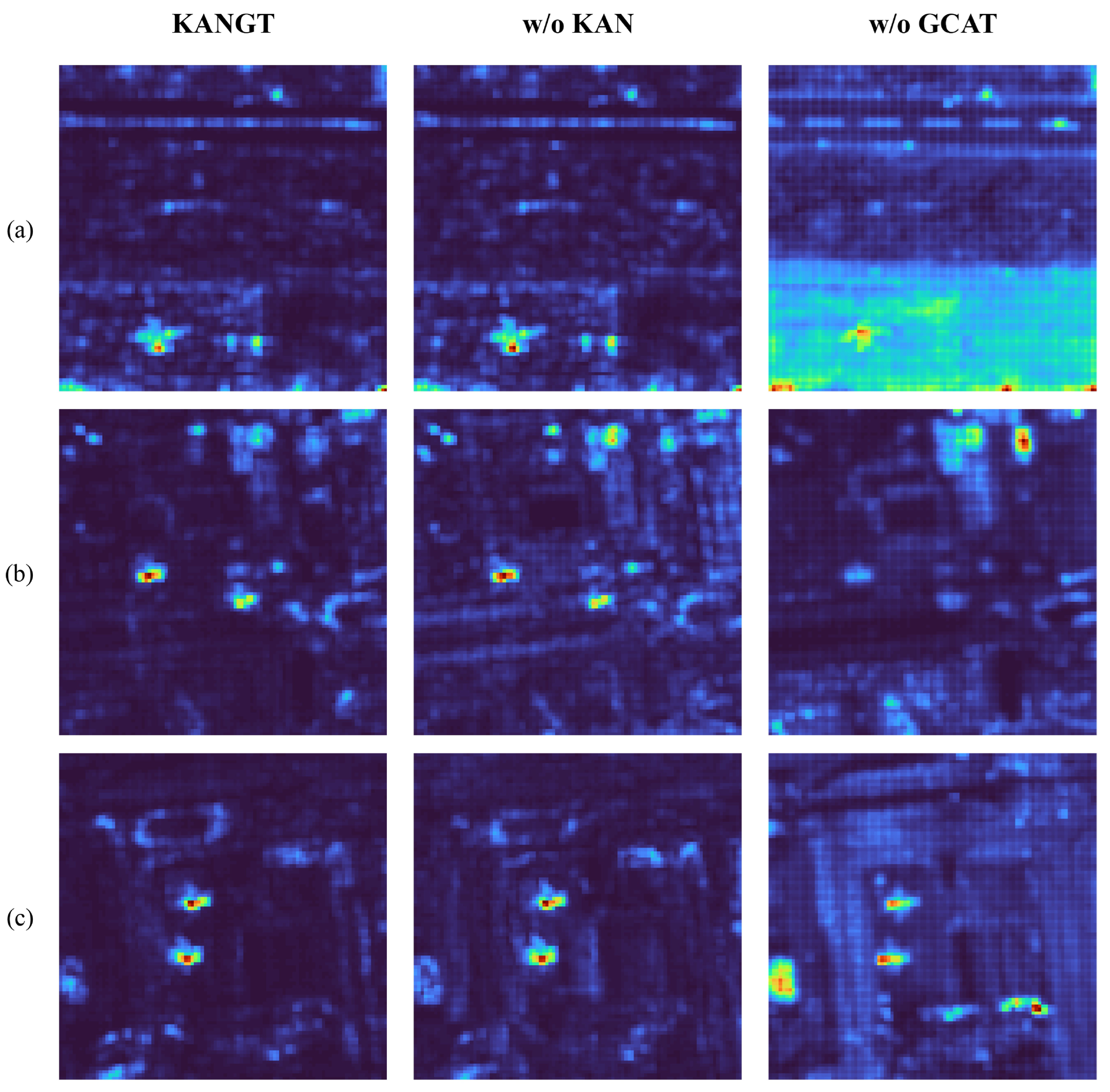
This section delves into ablation experiments conducted across eight distinct datasets to assess the individual impacts of KAN-MLP and GCAT. Firstly, while keeping all other GCAT components intact, we substitute KAN-MLP with a conventional MLP to construct our baseline model. Secondly, we remove the entire GCAT and replaced it with the standard global attention mechanism. We denote these models as the w/o KAN and w/o GCAT variants. All models are fairly compared using the same training period, batch size, and learning rate. Finally, the quantitative and visual results of ablation are reported in

Table 4. Quantitative results of ablation experiments on 8 datasets (AUC scores).

Dataset	KANGT	w/o KAN	w/o GCAT
ABU-Urban-4	0.9906	0.9882	0.9767
Cat Island	0.9994	0.9994	0.9639
Gulfport	0.9945	0.9937	0.9085
Los Angeles-1	0.9740	0.9468	0.8704
Los Angeles-2	0.9893	0.9878	0.9686
Pavia	0.9995	0.9994	0.9269
San Diego	0.9923	0.9909	0.9893
Texas Coast	0.9976	0.9965	0.9911
Average	0.9921	0.9883	0.9494

Bold values indicate the best performance on each dataset.

and Figure 9.

4.4.1. Effectiveness of KAN-MLP

The removal of the KAN-MLP module led to performance degradation on most datasets, but exceptions such as Pavia and Cat Island had a relatively small impact, indicating that KAN-MLP had a negligible effect on near-perfect AUC scores. In the complex scenarios composed of backgrounds such as Los Angeles-1, Los Angeles-2, and ABU-Urban-4, the performance degradation was more obvious. The AUC scores of the latter two decreased by 0.0043 and 0.0024, respectively. The abnormal heatmaps in Figure 9 were analyzed. Compared with the KANGT model, the w/o KAN model has a weaker background suppression ability, resulting in a noisier background in the detection results. This discovery highlights the crucial role of the Kolmogorov–Arnold Network in the feature extraction process. Its superior function approximation capability enables the model to describe complex spectral–spatial relationships more accurately, thereby learning more discriminative features and enhancing the discrimination between anomalies and backgrounds, which is particularly important in challenging heterogeneous environments.

4.4.2. Effectiveness of GCAT

The replacement of the GCAT mechanism with the standard global attention module led to a consistent and substantial decline in performance across all datasets, as illustrated in Table 4. This decline was particularly pronounced in the Los Angeles-1 and Gulfport datasets, where the AUC decreased by 0.0807 and 0.0860, respectively. Qualitatively, the abnormal heatmaps presented in Figure 9 indicate that the model without GCAT generates a significant number of false alarms in the background and fails to adequately distinguish anomalies, thereby accounting for the notable reduction in AUC. These findings highlight the crucial role of GCAT in the extraction of anomalies and the suppression of the background and can be regarded as an indispensable component of KANGT anomaly detection.

4.4.3. Computational Efficiency Analysis

A critical requirement for the practical deployment of HAD algorithms—particularly in onboard or real-time scenarios—is computational efficiency. The introduction of KANs, which involve B-spline evaluations, raises a legitimate concern regarding increased inference latency compared to simple MLPs. To address this, we conducted a rigorous quantitative analysis of the inference time for the KANGT model and its ablation variants.

Table 5. Quantitative results of ablation experiments on 8 datasets (time/s).

Dataset	KANGT	w/o KAN	w/o GCAT
ABU-Urban-4	35.43	28.41	27.61
Cat Island	38.21	28.58	27.74
Gulfport	33.91	23.11	21.56
Los Angeles-1	34.19	23.38	22.31
Los Angeles-2	34.18	22.71	20.83
Pavia	45.89	28.41	26.58
San Diego	33.59	23.21	22.72
Texas Coast	34.24	22.72	20.97
Average	36.21	25.07	23.79

presents the average running time (in seconds) for processing the complete test datasets on an NVIDIA GeForce RTX 3060 GPU. The w/o GCAT model, representing a standard Transformer backbone, averages 23.79 s. The w/o KAN model, which adds the GCAT mechanism but uses standard MLPs, averages 25.07 s. This indicates that the dual-branch gating mechanism introduces a negligible overhead (∼1.3 s), validating the efficiency of the CFMM router. The full KANGT model averages 36.21 s. The integration of KAN-MLP adds approximately 11 s to the total inference time compared to the MLP-based variant. This ∼44% increase is attributed to the computational cost of evaluating B-spline basis functions on the grid ($G=5$).

4.4.4. Summary

A comparative analysis of the two ablations reveals their distinct yet complementary strengths. The performance deficit from removing the KAN module is most acute in scenarios requiring sophisticated feature representation (e.g., Los Angeles-2 and ABU-Urban-4), affirming its role as a powerful feature extractor. Conversely, the performance penalty for removing the GCAT mechanism is severe in scenes with complex background clutter (e.g., Los Angeles-1 and Gulfport), highlighting its importance for adaptive spatial reasoning. In addition, the time efficiency analysis confirms that KANGT maintains a highly competitive inference speed (∼36 s) and the Auto-AD method typically requires about 30 s, while the LREN method can exceed 160 s for similar dataset sizes [52]. The proposed complete KANGT model, integrating both components, consistently achieves the highest or competitively high AUC scores across all datasets. It successfully bridges the gap between representational power and computational efficiency, delivering robust and practical anomaly detection performance.

4.5. Hyperparameter Sensitivity

In the proposed KANGT, the KAN-MLP serves as a core component for feature transformation. A critical hyperparameter within this module is the grid size, which controls the granularity of the spline functions and consequently influences the model’s capacity and flexibility. To systematically investigate its impact, we conducted experiments by setting the grid size as 3, 5, 7, and 10 on eight datasets. The AUC results are summarized in

Table 6. Hyperparameter sensitivity analysis on different datasets (AUC score). Select the grid size of KAN as a hyperparameter, with the grid sizes set to 3, 5, 7, and 10.

Dataset	Grid = 3	Grid = 5	Grid = 7	Grid = 10
ABU-Urban-4	0.9867	0.9906	0.9808	0.9854
Cat Island	0.9876	0.9994	0.9894	0.9850
Gulfport	0.9922	0.9945	0.9915	0.9891
Los Angeles-1	0.9681	0.9725	0.9666	0.9740
Los Angeles-2	0.9798	0.9824	0.9893	0.9830
Pavia	0.9991	0.9995	0.9991	0.9960
San Diego	0.9923	0.9917	0.9913	0.9916
Texas Coast	0.9970	0.9976	0.9970	0.9964

. As evidenced by the table, the model demonstrates a degree of robustness to changes in the grid size, with performance fluctuations across different datasets being relatively minor. Nonetheless, a clear pattern emerges: a grid size of 5 consistently yields superior or highly competitive results across the majority of the datasets, including ABU-Urban-4, Cat Island, Gulfport, Los Angeles-1, Los Angeles-2, Pavia, and Texas Coast. For instance, on the Cat Island dataset, the AUC score peaks at 0.9994 with grid = 5, significantly outperforming other configurations. This suggests that a grid size of 5 provides an optimal balance, offering sufficient representational power without leading to overfitting. While grid = 3 occasionally achieves commendable performance (e.g., on San Diego), it may underfit complex spectral structures in some scenarios. Conversely, larger grid sizes such as 7 and 10 do not confer consistent benefits and can even lead to a slight performance degradation, as observed in the results for Gulfport and Texas Coast, potentially due to increased model complexity. Based on this comprehensive analysis, we conclude that a grid size of 5 represents a robust and effective default setting for the KAN module in our anomaly detection framework. We suggest setting the grid to 5 and recommend this as a standard configuration for future applications.

While the grid size determines the resolution of the B-spline approximation, the spline order k is a fundamental structural hyperparameter that governs the smoothness and polynomial degree of the basis functions. The choice of k involves a critical trade-off between representational plasticity and model regularization. To strictly validate our default configuration, we extended the sensitivity analysis to evaluate the impact of spline order by varying $k\in \{2,3,4\}$ across all eight datasets, with the grid size fixed at the optimal setting of grid = 5. The quantitative results, summarized in

Table 7. Hyperparameter sensitivity analysis on different datasets (AUC score). Select the spline order of KAN as a hyperparameter, with the spline order k set to 2, 3, and 4.

Dataset	k = 2	k = 3	k = 4
ABU-Urban-4	0.9906	0.9906	0.9906
Cat-Island	0.9992	0.9994	0.9991
Gulfport	0.9943	0.9945	0.9944
Los Angeles-1	0.9705	0.9740	0.9711
Los Angeles-2	0.9886	0.9893	0.9882
Pavia	0.9994	0.9995	0.9994
San Diego	0.9923	0.9923	0.9922
Texas-Coast	0.9976	0.9976	0.9975

, reveal a consistent pattern: the cubic spline configuration ($k=3$) invariably achieves superior AUC scores compared to its quadratic ($k=2$) and quartic ($k=4$) counterparts. For instance, on the complex Los Angeles-2 dataset, the AUC improves from 0.9886 ($k=2$) to 0.9893 ($k=3$). Theoretically, this underscores the importance of $C^2$ continuity provided by cubic splines, which is essential for modeling the inherently smooth and continuous physical nature of hyperspectral signatures without introducing artificial discontinuities typical of lower-order approximations. Conversely, increasing the order to $k=4$ results in a slight performance degradation across most datasets (e.g., Los Angeles-1 drops from 0.9740 to 0.9711). We attribute this to the “over-reconstruction” phenomenon; the excessive flexibility of higher-order polynomials allows the network to inadvertently reconstruct sparse anomalies and fit high-frequency noise, thereby reducing the contrast in the anomaly detection map. Furthermore, higher spline orders incur a quadratic increase in computational complexity ($O\left(k^2\right)$). Therefore, $k=3$ represents the optimal operational point, maximizing the separability between the background and anomalies while maintaining computational efficiency and preventing overfitting.

5. Discussion

To thoroughly evaluate the generalization capability of the proposed KANGT model, we conducted a series of rigorous experiments focusing on cross-scenario generalization and noise robustness. The quantitative results are systematically presented in

Table 8. Cross-scenario generalization performance (AUC).

Training Dataset	Test Dataset	AUC
Los Angeles-1	Los Angeles-2	0.9666
Los Angeles-2	Los Angeles-2	0.9893
Los Angeles-2	Los Angeles-1	0.9472
Los Angeles-1	Los Angeles-1	0.9740

and

Table 9. Noise robustness analysis on Pavia (AUC).

Noise Type	(Level, AUC)	(Level, AUC)	(Level, AUC)	(Level, AUC)
Gaussian	(0.01, 0.9992)	(0.05, 0.9991)	(0.1, 0.9984)	(0.2, 0.9813)
Salt-and-Pepper	(0.01, 0.9967)	(0.02, 0.9804)	(0.03, 0.9233)	(0.05, 0.8876)

to provide a clear and comprehensive performance overview.

The cross-scenario generalization capability was assessed through a cross-dataset validation strategy, where the model was trained on one dataset and tested on another without any fine-tuning. The network’s layer channels depend on the bands in the input hyperspectral imaging data. Thus, the Los Angeles-1 and Los Angeles-2 datasets, possessing identical band counts, are the only two among the eight HSI collections appropriate for cross-validation studies. As summarized in Table 8, KANGT demonstrated strong transferability. When trained on Los Angeles-1 and tested on the unseen Los Angeles-2 dataset, it achieved a high AUC of 0.9666. Conversely, the model trained on Los Angeles-2 attained an AUC of 0.9472 on Los Angeles-1. These results confirm that the feature representations learned by KANGT possess strong robustness to geographical and contextual variations between different hyperspectral scenes.

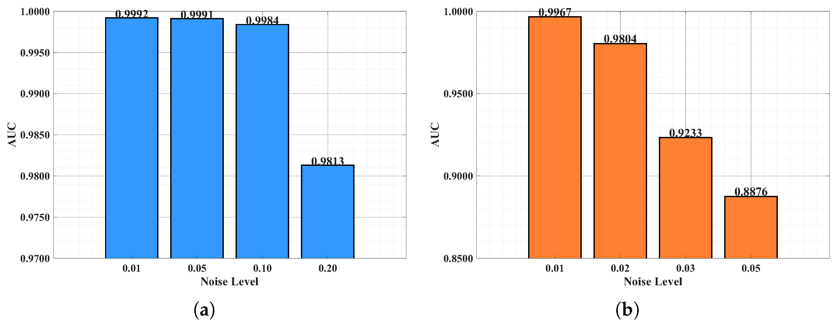
We further investigated the model’s robustness against two common types of noise: Gaussian noise [57] and salt-and-pepper noise [58]. The performance under varying noise levels is detailed in Table 9 and Figure 10. KANGT exhibited exceptional resilience to Gaussian noise. Even at a high noise level of 0.2, it maintained a commendable AUC of 0.9813, with only a minimal performance drop from 0.9992 (at level 0.01). For salt-and-pepper noise, the model showed strong resistance to low-level corruption (AUC = 0.9967 at level 0.01). Although performance decreased more noticeably at higher noise intensities, this is consistent with the destructive nature of salt-and-pepper noise, which randomly corrupts individual pixels. The model’s superior performance, especially under Gaussian noise, underscores its suitability for practical applications where such perturbations are common.

6. Conclusions

In this paper, we present the Synergistic Kolmogorov–Arnold Network and Fidelity-Gated Transformer, a novel framework for HAD systematically addressing two core limitations: macro-level “uniform processing” and micro-level “fixed activation”. The architecture achieves this through two synergistic innovations: the Fidelity-Gated Context-Aware Transformer, utilizing a fidelity-based gating module to explicitly separate data streams, and the KAN-MLP, which replaces traditional FFNs with learnable, spline-based functions for superior non-linear approximation. KANGT’s state-of-the-art performance is demonstrated through extensive experiments on eight HSI datasets, showing superior background suppression and enhanced anomaly–background separability. Rigorous ablation studies validate this synergistic design, confirming that the GCAT and KAN-MLP modules provide unique and indispensable contributions.

This framework establishes a new paradigm for HAD. However, we acknowledge a limitation regarding the scale of validation, which is a general constraint within the current unsupervised HAD research landscape due to the scarcity of reliable pixel-level annotations for large-scale scenes. While our experiments on eight challenging benchmarks provide rigorous validation of KANGT’s theoretical contributions, future work will aim to expand the evaluation to larger scenarios, potentially leveraging semi-supervised techniques to overcome annotation scarcity. Additionally, we will continue to address the computational efficiency of KANs to balance high precision with real-time application demands.

References

1. Su, H.; Wu, Z.; Zhang, H.; Du, Q. Hyperspectral anomaly detection: A survey. IEEE Geosci. Remote Sens. Mag. 2021, 10, 64–90. [Google Scholar] [CrossRef]
2. Plaza, A.; Benediktsson, J.A.; Boardman, J.W.; Brazile, J.; Bruzzone, L.; Camps-Valls, G.; Chanussot, J.; Fauvel, M.; Gamba, P.; Gualtieri, A.; et al. Recent advances in techniques for hyperspectral image processing. Remote Sens. Environ. 2009, 113, S110–S122. [Google Scholar] [CrossRef]
3. Chen, C.; Cao, J.; Wang, T.; Su, Y.; Wang, N.; Zhang, C.; Zhu, L.; Zhang, L. GLFFEN: A Global–Local Feature Fusion Enhancement Network for Hyperspectral Image Classification. Remote Sens. 2025, 17, 3705. [Google Scholar] [CrossRef]
4. Wang, N.; Cui, Z.; Lan, Y.; Zhang, C.; Xue, Y.; Su, Y.; Li, A. Large-Scale Hyperspectral Image-Projected Clustering via Doubly Stochastic Graph Learning. Remote Sens. 2025, 17, 1526. [Google Scholar] [CrossRef]
5. Hu, X.; Xie, C.; Fan, Z.; Duan, Q.; Zhang, D.; Jiang, L.; Wei, X.; Hong, D.; Li, G.; Zeng, X.; et al. Hyperspectral anomaly detection using deep learning: A review. Remote Sens. 2022, 14, 1973. [Google Scholar] [CrossRef]
6. Reed, I.S.; Yu, X. Adaptive multiple-band CFAR detection of an optical pattern with unknown spectral distribution. IEEE Trans. Acoust. Speech Signal Process. 2002, 38, 1760–1770. [Google Scholar] [CrossRef]
7. Kwon, H.; Nasrabadi, N.M. Kernel RX-algorithm: A nonlinear anomaly detector for hyperspectral imagery. IEEE Trans. Geosci. Remote Sens. 2005, 43, 388–397. [Google Scholar] [CrossRef]
8. Li, L.; Li, W.; Qu, Y.; Zhao, C.; Tao, R.; Du, Q. Prior-based tensor approximation for anomaly detection in hyperspectral imagery. IEEE Trans. Neural Netw. Learn. Syst. 2020, 33, 1037–1050. [Google Scholar] [CrossRef]
9. Wang, M.; Wang, Q.; Hong, D.; Roy, S.K.; Chanussot, J. Learning tensor low-rank representation for hyperspectral anomaly detection. IEEE Trans. Cybern. 2022, 53, 679–691. [Google Scholar] [CrossRef] [PubMed]
10. Wang, N.; Cui, Z.; Li, A.; Xue, Y.; Wang, R.; Nie, F. Multi-order graph based clustering via dynamical low rank tensor approximation. Neurocomputing 2025, 647, 130571. [Google Scholar] [CrossRef]
11. Wang, S.; Wang, X.; Zhang, L.; Zhong, Y. Auto-AD: Autonomous hyperspectral anomaly detection network based on fully convolutional autoencoder. IEEE Trans. Geosci. Remote Sens. 2021, 60, 5503314. [Google Scholar] [CrossRef]
12. Jiang, T.; Li, Y.; Xie, W.; Du, Q. Discriminative reconstruction constrained generative adversarial network for hyperspectral anomaly detection. IEEE Trans. Geosci. Remote Sens. 2020, 58, 4666–4679. [Google Scholar] [CrossRef]
13. Wang, D.; Zhuang, L.; Gao, L.; Sun, X.; Huang, M.; Plaza, A. BockNet: Blind-block reconstruction network with a guard window for hyperspectral anomaly detection. IEEE Trans. Geosci. Remote Sens. 2023, 61, 5531916. [Google Scholar] [CrossRef]
14. Fu, X.; Jia, S.; Zhuang, L.; Xu, M.; Zhou, J.; Li, Q. Hyperspectral anomaly detection via deep plug-and-play denoising CNN regularization. IEEE Trans. Geosci. Remote Sens. 2021, 59, 9553–9568. [Google Scholar] [CrossRef]
15. Zhao, M.; Zheng, W.; Hu, J. HTC-HAD: A Hybrid Transformer-CNN Approach for Hyperspectral Anomaly Detection. IEEE J. Sel. Top. Appl. Earth Obs. Remote Sens. 2025, 18, 10144–10156. [Google Scholar] [CrossRef]
16. Fu, X.; Zhang, T.; Cheng, J.; Jia, S. MMR-HAD: Multi-scale Mamba Reconstruction Network for Hyperspectral Anomaly Detection. IEEE Trans. Geosci. Remote Sens. 2025, 63, 5516914. [Google Scholar] [CrossRef]
17. Zhang, J.; Xiang, P.; Teng, X.; Zhao, D.; Li, H.; Song, J.; Zhou, H.; Tan, W. Enhancing hyperspectral anomaly detection with a novel differential network approach for precision and robust background suppression. Remote Sens. 2024, 16, 434. [Google Scholar] [CrossRef]
18. Guo, T.; He, L.; Luo, F.; Gong, X.; Li, Y.; Zhang, L. Anomaly detection of hyperspectral image with hierarchical antinoise mutual-incoherence-induced low-rank representation. IEEE Trans. Geosci. Remote Sens. 2023, 61, 5510213. [Google Scholar] [CrossRef]
19. Yang, N.; Jia, X.; Hu, C.; Zhang, Y.; Lyu, L. A dual-branch encoder context-aware fusion network for ultrasound image segmentation. Appl. Soft Comput. 2025, 182, 113538. [Google Scholar] [CrossRef]
20. Liu, Z.; Wang, Y.; Vaidya, S.; Ruehle, F.; Halverson, J.; Soljačić, M.; Hou, T.Y.; Tegmark, M. Kan: Kolmogorov-arnold networks. arXiv 2024, arXiv:2404.19756. [Google Scholar]
21. Wu, Z.; Lu, H.; Paoletti, M.E.; Su, H.; Jing, W.; Haut, J.M. KACNet: Kolmogorov-Arnold Convolution Network for Hyperspectral Anomaly Detection. IEEE Trans. Geosci. Remote Sens. 2025, 63, 5506514. [Google Scholar] [CrossRef]
22. Fascista, A. Toward integrated large-scale environmental monitoring using WSN/UAV/Crowdsensing: A review of applications, signal processing, and future perspectives. Sensors 2022, 22, 1824. [Google Scholar] [CrossRef] [PubMed]
23. Peng, J.; Sun, W.; Li, H.C.; Li, W.; Meng, X.; Ge, C.; Du, Q. Low-rank and sparse representation for hyperspectral image processing: A review. IEEE Geosci. Remote Sens. Mag. 2021, 10, 10–43. [Google Scholar] [CrossRef]
24. Pant, A.; Baniya, A.A.; Lee, T.K.; Aryal, S. Hyperspectral Anomaly Detection Methods: A Survey and Comparative Study. arXiv 2025, arXiv:2507.05730. [Google Scholar] [CrossRef]
25. Zhang, L.; Cheng, B.; Lin, F. Hyperspectral anomaly detection via fractional Fourier transform and deep belief networks. Infrared Phys. Technol. 2022, 125, 104314. [Google Scholar] [CrossRef]
26. Xiao, S.; Zhang, T.; Xu, Z.; Qu, J.; Hou, S.; Dong, W. Anomaly detection of hyperspectral images based on transformer with spatial–spectral dual-window mask. IEEE J. Sel. Top. Appl. Earth Obs. Remote Sens. 2023, 16, 1414–1426. [Google Scholar] [CrossRef]
27. Cao, H.; Tan, C.; Gao, Z.; Xu, Y.; Chen, G.; Heng, P.A.; Li, S.Z. A survey on generative diffusion models. IEEE Trans. Knowl. Data Eng. 2024, 36, 2814–2830. [Google Scholar] [CrossRef]
28. Ma, J.; Xie, W.; Shi, Y.; Xiang, X.; Li, Y.; Fang, L. BSDM: Background suppression diffusion model for hyperspectral anomaly detection. IEEE Trans. Circuits Syst. Video Technol. 2025, 1. [Google Scholar] [CrossRef]
29. Wu, Y.; Meng, Y.; Sun, L. Diffusing background dictionary for hyperspectral anomaly detection. In Proceedings of the Asian Conference on Computer Vision, Hanoi, Vietnam, 8–12 December 2024; pp. 1046–1064. [Google Scholar]
30. Chen, W.; Zhi, X.; Jiang, S.; Huang, Y.; Han, Q.; Zhang, W. Dwsdiff: Dual-window spectral diffusion for hyperspectral anomaly detection. IEEE Trans. Geosci. Remote Sens. 2025, 63, 5504617. [Google Scholar] [CrossRef]
31. He, X.; Zhou, S.; Ling, Q.; Li, M.; Li, Z.; Zhang, Y.; Lin, Z. Global-to-local spatial–spectral awareness transformer network for hyperspectral anomaly detection. IEEE Trans. Geosci. Remote Sens. 2024, 62, 5530422. [Google Scholar] [CrossRef]
32. Deng, L.; Zhou, B.; Chen, Y.; Li, Z. Dual-window transformer framework with pyramid structure and constrained self-attention for hyperspectral anomaly detection. J. Eur. Opt. Soc.-Rapid Publ. 2025, 21, 43. [Google Scholar] [CrossRef]
33. Alzubaidi, L.; Zhang, J.; Humaidi, A.J.; Al-Dujaili, A.; Duan, Y.; Al-Shamma, O.; Santamaría, J.; Fadhel, M.A.; Al-Amidie, M.; Farhan, L. Review of deep learning: Concepts, CNN architectures, challenges, applications, future directions. J. Big Data 2021, 8, 53. [Google Scholar] [CrossRef]
34. Vaswani, A.; Shazeer, N.; Parmar, N.; Uszkoreit, J.; Jones, L.; Gomez, A.N.; Kaiser, Ł.; Polosukhin, I. Attention is all you need. Adv. Neural Inf. Process. Syst. 2017, 30. [Google Scholar]
35. Liu, L.; Liu, J.; Yuan, S.; Slabaugh, G.; Leonardis, A.; Zhou, W.; Tian, Q. Wavelet-based dual-branch network for image demoiréing. In Proceedings of the European Conference on Computer Vision, Glasgow, UK, 23–28 August 2020; Springer: Berlin/Heidelberg, Germany, 2020; pp. 86–102. [Google Scholar]
36. Chung, J.; Gulcehre, C.; Cho, K.; Bengio, Y. Gated feedback recurrent neural networks. In Proceedings of the International Conference on Machine Learning. PMLR, Lille, France, 6–11 July 2015; pp. 2067–2075. [Google Scholar]
37. Kruse, R.; Mostaghim, S.; Borgelt, C.; Braune, C.; Steinbrecher, M. Multi-layer perceptrons. In Computational Intelligence: A Methodological Introduction; Springer: Berlin/Heidelberg, Germany, 2022; pp. 53–124. [Google Scholar]
38. Fernandez, A. TeLU Activation Function for Fast and Stable Deep Learning. Master’s thesis, University of South Florida, Tampa, FL, USA, 2024. [Google Scholar]
39. Liu, Z.; Ma, P.; Wang, Y.; Matusik, W.; Tegmark, M. Kan 2.0: Kolmogorov-arnold networks meet science. arXiv 2024, arXiv:2408.10205. [Google Scholar] [CrossRef]
40. Somvanshi, S.; Javed, S.A.; Islam, M.M.; Pandit, D.; Das, S. A survey on kolmogorov-arnold network. ACM Comput. Surv. 2025, 58, 1–35. [Google Scholar] [CrossRef]
41. Shiraishi, H.; Ishibuchi, H.; Nakata, M. X-KAN: Optimizing Local Kolmogorov-Arnold Networks via Evolutionary Rule-Based Machine Learning. arXiv 2025, arXiv:2505.14273. [Google Scholar]
42. Yu, R.; Yu, W.; Wang, X. Kan or mlp: A fairer comparison. arXiv 2024, arXiv:2407.16674. [Google Scholar] [CrossRef]
43. Beatrize, J.; Vieira, L.M.; Chen, A.; Grünwald, T. The Kolmogorov-Arnold Renaissance: Scalable, Symbolic, and Interpretable Neural Networks 2025. Available online: https://hal.science/hal-05032047/ (accessed on 1 December 2025).
44. Noorizadegan, A.; Wang, S.; Ling, L. A Practitioner’s Guide to Kolmogorov-Arnold Networks. arXiv 2025, arXiv:2510.25781. [Google Scholar]
45. Li, S.; Song, W.; Fang, L.; Chen, Y.; Ghamisi, P.; Benediktsson, J.A. Deep learning for hyperspectral image classification: An overview. IEEE Trans. Geosci. Remote Sens. 2019, 57, 6690–6709. [Google Scholar] [CrossRef]
46. Grewal, R.; Kasana, S.S.; Kasana, G. Hyperspectral image segmentation: A comprehensive survey. Multimed. Tools Appl. 2023, 82, 20819–20872. [Google Scholar] [CrossRef]
47. Seydi, S.T.; Bozorgasl, Z.; Chen, H. Unveiling the power of wavelets: A wavelet-based kolmogorov-arnold network for hyperspectral image classification. arXiv 2024, arXiv:2406.07869. [Google Scholar]
48. Wang, C.; Zhang, X.; Liu, L. FloodKAN: Integrating Kolmogorov–Arnold Networks for Efficient Flood Extent Extraction. Remote Sens. 2025, 17, 564. [Google Scholar] [CrossRef]
49. Köksoy, O. Multiresponse robust design: Mean square error (MSE) criterion. Appl. Math. Comput. 2006, 175, 1716–1729. [Google Scholar] [CrossRef]
50. Liu, J.; Hou, Z.; Li, W.; Tao, R.; Orlando, D.; Li, H. Multipixel anomaly detection with unknown patterns for hyperspectral imagery. IEEE Trans. Neural Netw. Learn. Syst. 2021, 33, 5557–5567. [Google Scholar] [CrossRef]
51. Tu, B.; Yang, X.; He, W.; Li, J.; Plaza, A. Hyperspectral anomaly detection using reconstruction fusion of quaternion frequency domain analysis. IEEE Trans. Neural Netw. Learn. Syst. 2023, 35, 8358–8372. [Google Scholar] [CrossRef] [PubMed]
52. Lian, J.; Wang, L.; Sun, H.; Huang, H. GT-HAD: Gated transformer for hyperspectral anomaly detection. IEEE Trans. Neural Netw. Learn. Syst. 2024, 36, 3631–3645. [Google Scholar] [CrossRef]
53. Jiang, K.; Xie, W.; Lei, J.; Jiang, T.; Li, Y. LREN: Low-rank embedded network for sample-free hyperspectral anomaly detection. In Proceedings of the AAAI Conference on Artificial Intelligence, Virtually, 19–21 May 2021; Volume 35, pp. 4139–4146. [Google Scholar]
54. Cheng, X.; Huo, Y.; Lin, S.; Dong, Y.; Zhao, S.; Zhang, M.; Wang, H. Deep feature aggregation network for hyperspectral anomaly detection. IEEE Trans. Instrum. Meas. 2024, 73, 5033016. [Google Scholar] [CrossRef]
55. Wang, H.; Yang, M.; Zhang, T.; Tian, D.; Wang, H.; Yao, D.; Meng, L.; Shen, H. Hyperspectral Anomaly Detection with Differential Attribute Profiles and Genetic Algorithms. Remote Sens. 2023, 15, 1050. [Google Scholar] [CrossRef]
56. Zhang, X.; Gao, K.; Wang, J.; Hu, Z.; Wang, H.; Wang, P. Siamese network ensembles for hyperspectral target detection with pseudo data generation. Remote Sens. 2022, 14, 1260. [Google Scholar] [CrossRef]
57. Russo, F. A method for estimation and filtering of Gaussian noise in images. IEEE Trans. Instrum. Meas. 2003, 52, 1148–1154. [Google Scholar] [CrossRef]
58. Azzeh, J.; Zahran, B.; Alqadi, Z. Salt and pepper noise: Effects and removal. JOIV Int. J. Inform. Vis. 2018, 2, 252–256. [Google Scholar] [CrossRef]
Figure 1. Architectural overview of KANGT. The network employs a Transformer-based structure trained on HSI cubes, with detection performed through reconstruction error analysis.
Remotesensing 17 03981 g001
Figure 2. The structure of the KAN-MLP module. The architecture leverages a dual-path design fusing a SiLU-based regularization branch with a learnable B-spline branch to achieve adaptive non-linear feature transformation. The default grid size is set as 5 and the spline order is 3.
Remotesensing 17 03981 g002
Figure 3. Methods of modeling the features of the LARB.
Remotesensing 17 03981 g003
Figure 4. CFMM methodology. The gating unit regulates LARB and GBRB activation during instruction, with its functional modes governed by the CFMM.
Remotesensing 17 03981 g004
Figure 5. Visual comparison of hyperspectral anomaly detection heatmaps across four datasets: (a) ABU-Urban-4, (b) Cat Island, (c) Gulfport, and (d) Los Angeles-1. The rows display the detection results for the proposed KANGT framework alongside state-of-the-art comparison methods (RX, 2S-GLRT, MsRFQFT, GT-HAD, PCA-TLRSR, DFAN, Auto-AD, and LREN) and the Ground Truth.
Remotesensing 17 03981 g005
Figure 6. Visual comparison of hyperspectral anomaly detection heatmaps across four datasets: (a) Los Angeles-2, (b) Pavia, (c) San Diego and (d) Texas Coast. The rows display the detection results for the proposed KANGT framework alongside state-of-the-art comparison methods (RX, 2S-GLRT, MsRFQFT, GT-HAD, PCA-TLRSR, DFAN, Auto-AD, and LREN) and the Ground Truth.
Remotesensing 17 03981 g006
Figure 7. HAD method separability visualization across 8 datasets. (a) ABU-Urban-4. (b) Cat Island. (c) Gulfport. (d) Los Angeles-1. (e) Los Angeles-2. (f) Pavia. (g) Sandiego. (h) Texas Coast.
Remotesensing 17 03981 g007
Figure 8. Two-dimensional ROC curves for 9 methods across 8 datasets. (a) ABU-Urban-4. (b) Cat Island. (c) Gulfport. (d) Los Angeles-1. (e) Los Angeles-2. (f) Pavia. (g) San Diego. (h) Texas Coast.
Remotesensing 17 03981 g008
Figure 9. Visualization of ablation study on three datasets. KANGT is the model proposed, w/o KAN is replacing KAN-MLP with a traditional MLP, and w/o GCAT is replacing GCAT with the standard global attention mechanism. (a) Gulfport. (b) Los Angeles-1. (c) Los Angeles-2.
Remotesensing 17 03981 g009
Figure 10. Noise robustness analysis on Pavia (AUC). (a) Guassian. (b) Salt-and-pepper.
Remotesensing 17 03981 g010