Spatial Consistency and Accuracy Assessment of Grassland Classification in the Sanjiangyuan Region: From Six Medium Resolution Land Cover Products

Highlights

What are the main findings?

• Evaluation of six global medium-resolution land cover products for grassland mapping in the Sanjiangyuan Region.
• Highest accuracy of ESA and FROM_GLC10, and lowest performance of Dynamic World, with results influenced by topography.

What are the implications of the main finding?

• Reliable reference for selecting suitable products for alpine grassland monitoring.
• Guidance for product fusion and fine-scale classification in high-altitude ecosystems.

Abstract

The Sanjiangyuan Region (SJYR), located in the core of the Qinghai–Tibet Plateau, is a key ecological barrier where grasslands, the dominant land cover, are undergoing continuous degradation due to climate change and human activities. Accurate characterization of grassland is essential for ecological monitoring, yet existing land-cover products show substantial discrepancies in alpine environments. This study systematically evaluated the spatial consistency and accuracy of six publicly medium resolution land cover products: GLC_FCS30, GlobeLand30, FROM_GLC10, ESA WorldCover (ESA), ESRI Land Cover (ESRI), and Dynamic World. We evaluated these products by comparing them with the Third National Land Survey data, performing Jaccard similarity and spatial consistency analyses, and validating their accuracy using five metrics: Overall Accuracy (OA), Producer’s Accuracy (PA), User’s Accuracy (UA), F1-score, and Matthews Correlation Coefficient (MCC). Results show large variations in estimated grassland area, ranging from 91,105 km² (Dynamic World) to 325,669 km² (GLC_FCS30). Pixel-level comparison revealed significant spatial heterogeneity, with only 54.3% of the region showing the desired high consistency. Accuracy validation indicated that ESA achieved the best classification results (OA = 74.24%, MCC = 0.80), while Dynamic World performed the worst (OA = 57.45%, F1 = 0.28). These products showed lower consistency in high-altitude western areas, and classification accuracy for most products varied with elevation and slope, indicating that topographic factors significantly influence remote sensing classification capabilities. These results provide a quantitative basis for product selection in the SJYR and highlight the need for improved calibration, data fusion, and classification approaches that better account for sparse vegetation and complex topography.

1. Introduction

Grassland ecosystems are widely distributed, and are one of the most important terrestrial ecosystems in China and the world [1,2]. Grassland not only plays a significant ecological role in water conservation, soil and water conservation, and wind prevention and sand fixation, but also serves as a key barrier for maintaining biodiversity and regulating regional climate [3,4]. In recent years, grassland ecosystems have been severely damaged [5,6,7,8] due to human activities, including climate change and overgrazing [9]. This has led to a persistent issue of grassland degradation in the Qinghai-Tibet Plateau region [10]. The Qinghai-Tibet Plateau is one of the world’s most significant areas for grassland and pasture distribution [2]. As the hinterland of this plateau [11], the Sanjiangyuan Region (SJYR) holds significant strategic value for China’s ecological security and regional sustainable development. With the continued advancement of the National Park System and the environmental civilization strategy [12,13], China has implemented a series of ecological protection measures in the SJYR aimed at safeguarding its endangered flora and fauna and its fragile ecosystems. Consequently, grassland resource management in the SJYR has received increasing attention [14]. As the core area of ecological security on the Qinghai-Tibet Plateau, the SJYR has a typical high-altitude, cold climate [15], with complex terrain and poor transportation, making large-scale, systematic field surveys of grassland resources challenging. Accordingly, satellite remote sensing represents the most feasible and practical approach for large-scale land cover monitoring and grassland classification [16].

In recent years, with the continuous improvement of remote sensing technology and the continuous enhancement in the spatial, temporal, and spectral resolutions of satellite sensors [17,18], the accuracy and timeliness of surface information acquisition have significantly improved, providing reliable support for achieving dynamic monitoring of global land cover and environmental changes [19]. The academic community has released a variety of global and regional-scale land cover products. Researchers primarily released early global land cover datasets at a spatial resolution of 1 km. Notable examples include the IGBP DISCover (1992–1993), developed based on AVHRR data by USGS [20]; the UMD Land Cover (1992–1993), produced by the University of Maryland [21], and the GLC2000 (2000), led by the European Space Agency (ESA) [22]. These products provided an initial reference framework for understanding global land cover patterns. Subsequently, land cover products with spatial resolutions of 500 m and 250 m were introduced, such as NASA’s MODIS series MCD12Q1 (2001-present, annually) [23] and ESA’s GlobCover (2005–2009) [24]. These medium-resolution products strike a better balance between accuracy and coverage, and are of great value in large-scale dynamic monitoring [25]. In recent years, multiple research institutions have successively released land cover products with higher spatial resolution. The National Geomatics Center of China (NGCC) led the development of the GlobeLand30 with a 30 m resolution [26]; the Aerospace Information Research Institute of the Chinese Academy of Sciences (CAS, AIR) released the GLC_FCS30 fine classification product with 30-m resolution [27]; Tsinghua University introduced the FROM_GLC series, with the 2010 version at 30 m resolution and an updated 2017 version improved to 10 m [28,29]; The European Space Agency (ESA) released the ESA WorldCover (ESA) at 10 m resolution, based on Sentinel-1/2 imagery [30]; ESRI collaborated with Impact Observatory and Microsoft to launch the ESRI Land Cover (ESRI) product with 10 m spatial resolution [31]; Additionally, the Dynamic World product launched on the Google Earth Engine platform in 2021, offers near real-time (NRT) update capability, enabling rapid response to land surface changes with flexible temporal resolution and a high degree of automated classification efficiency [32]. By utilizing high-resolution spatial data, it is possible to identify more detailed spatial features, particularly capturing small-scale characteristics and changes in heterogeneous landscapes [33]. It is worth noting that the current global landscape offers a wide range of medium resolution land cover products from diverse sources, providing crucial data support for grassland resource monitoring.

However, these land cover products exhibit significant differences in classification systems, remote sensing data sources, spatial resolution, and modelling methods, leading to inconsistencies and variations in classification accuracy, which in turn affects their reliability in practical applications [34,35]. Therefore, the scientific community has conducted a series of evaluation studies on various products, highlighting differences in their applicability across different regions and specific land types. For example, Yang et al. compared the classification accuracy of seven global land cover datasets with different resolutions, including IGBP DISCover, UMD LC, GLC, MCD12Q1, GLCNMO, CCI-LC, and GlobeLand30 in China. The results revealed significant differences among these products in land cover area estimation and spatial distribution patterns [36]. Xu et al. evaluated the accuracy of three 10 m global products, ESA, Dynamic World, and ESRI, at the global scale. The results indicated that ESA demonstrated the highest overall accuracy, followed by Dynamic World and ESRI. Additionally, the accuracy of all three products decreased in landscapes with high surface heterogeneity [37]. In the Qinghai-Tibet Plateau, where terrain is highly rugged and surface heterogeneity is high, misclassification and confusion issues are more pronounced, resulting in substantial uncertainty. Pan et al. assessed the consistency and accuracy of five products—MCD12Q1, C3S-LC, GlobeLand30, GLC_FCS30, and ESA2020 in plateau regions. The results showed that there were significant differences in grassland coverage areas among different products, and the consistency in grassland and bare land transitional zones was relatively low [25]. Cai et al. analyzed the consistency of MCD12Q1, CCI-LC, GlobeLand30, and CNLUCC in the Qinghai-Tibet Plateau, and it was found that the average spatial consistency among products decreased with increasing elevation [38]. Zhang et al. evaluated 15 land cover products in the Nyingchi and Shannan regions, revealing that grasslands were prone to confusion with bare land and shrub classifications, and product accuracy was susceptible to topographic influences [39]. Overall, existing research indicates that land cover products in plateau regions exhibit generally low classification accuracy, with results being susceptible to complex topography and surface heterogeneity. However, specialized studies on grassland categories remain scarce, notably lacking systematic comparisons of different products’ accuracy in grassland identification. As the core region of the Qinghai-Tibet Plateau, the SJYR holds significant importance for understanding the patterns and changes of alpine ecosystems through dynamic monitoring of its grassland resources. A systematic evaluation of the spatial consistency and accuracy of grassland classification across different products in this region is essential to reveal their respective strengths and limitations in alpine grassland monitoring. This assessment will provide valuable references for optimizing regional grassland extraction methods and enhancing grassland monitoring practices.

This study focuses on the typical alpine grassland ecosystems in the SJYR, conducting spatial consistency and accuracy assessments of the following six land cover products: GlobeLand30, GLC_FCS30, FROM_GLC10, ESA, ESRI, and Dynamic World. Moreover, by analyzing trends in consistency and classification accuracy across different elevation and slope intervals, the study reveals the impact of SJYR’s complex terrain on classification outcomes. Additionally, this research delves into the underlying causes of uncertainty in product classification results and proposes targeted improvement strategies, such as enhancing terrain correction, data fusion, and optimizing category definitions. These findings not only provide a reliable data assessment framework for monitoring grassland resources in the SJYR but also offer pathways for multi-source remote sensing product fusion, algorithm optimization, and classification system refinement in plateau regions.

2. Materials and Methods

2.1. Study Area

The SJYR is located in the Qinghai-Tibet Plateau, in the southern part of Qinghai Province, with geographical coordinates ranging from 89°24′E to 102°23′E and 31°39′N to 36°16′N. The region has an average elevation of approximately 4000 m and covers an area of about 395,000 km², encompassing 21 counties across four prefectures (Figure 1).

The terrain is highly complex and diverse, characterized by snow-covered mountains and glacier systems in the west, and plateau river valleys, wetlands, and alluvial plains in the east. Importantly, the SJYR contains the headwaters of China’s three major rivers—the Yellow River, Yangtze River, and Lancang River—hence the name “Sanjiangyuan” (literally “the Source of Three Rivers”). These river source regions form a dense hydrological network and serve as a critical ecological barrier for national water security. The climate is typical plateau continental, with strong and prolonged solar radiation, low air pressure, thin atmosphere, and low temperatures [40]. Precipitation is concentrated in the summer months, while the growing season of alpine vegetation is short, lasting only about 90 to 120 days [41].

The SJYR is a vital reservoir of genetic diversity on the Qinghai-Tibet Plateau. It serves as a core habitat for iconic plateau species such as the Tibetan antelope (Pantholops hodgsonii), Tibetan gazelle (Procapra picticaudata), and wild yak (Bos mutus) [42]. It is also the core area of China’s ecological security barrier [43]. The region has vast grassland areas, primarily consisting of alpine meadows and alpine steppes. Alpine meadows feature a dominance of perennial herbaceous species like Kobresia pygmaea and Kobresia humilis, which exhibit higher vegetation cover and biomass. In contrast, alpine steppes are mainly composed of Carex moorcroftii and Stipa purpurea, featuring simpler vegetation structure, lower coverage and a relatively brief growing season [42,44].

2.2. Data

2.2.1. Publicly Available Land Cover Products

To scientifically evaluate the applicability and consistency of multi-source remote sensing land cover products for grassland classification in the SJYR, this study selected six representative global products: GLC_FCS30 [27], GlobeLand30 [26], FROM_GLC10 [29], ESA [30], ESRI [31] and Dynamic World [32]. These products were chosen because they provide globally accessible, contemporary 10–30 m land cover information suitable for characterizing the heterogeneous alpine grasslands of the region. Collectively, they encompass diverse sensing sources, temporal baselines, and modelling approaches, enabling a comprehensive assessment of how different data inputs and methodological frameworks influence grassland delineation (

Table 1. Overview of six global land cover products used in this study.

Dataset	Satellites	Resolution	Period	Institution	Classification System	Method
GLC_FCS30	Landsat	30 m	1985–2022	AIR	35 classes of the fine system	Random forest
GlobeLand30	Landsat TM/ETM+,	30 m	2000, 2010, 2020	NGCC	10 classes	Pixel-bject–Knowledge (POK)
	HJ-1,
	GF-1 WFV
FROM_GLC10	Sentinel-2	10 m	2017	THU	10 classes	Random forest
ESA	Sentinel-1/2	10 m	2020, 2021	ESA	11 classes of LCCS	Gradient boosting decision tree (CatBoost)
ESRI	Sentinel-2	10 m	2017–2024	Esri&Impact Observatory	9 classes	Convolutional Neural Network—UNet
Dynamic World	Sentinel-2	10 m	Near Real-Time	Google&WRI	9 classes of probability maps	Fully Convolutional Neural Network (FCNN)

). All six products include grassland-related categories. Nevertheless, due to differences in classification systems, the specific definitions of grassland vary across products (

Table 2. Definitions of “grassland”-related categories across the six land cover products.

Dataset	Class	Code	Description
GLC_FCS30	Grassland	130	Herbaceous cover percentage classification to >15%.
GlobeLand30	Grassland	30	Land covered by natural herbaceous vegetation with a cover of more than 10%, including grasslands, meadows, savannas, desert grasslands, and urban artificial grasslands.
FROM_GLC10	Grassland	30	Herbaceous cover percentage classification to >15%.
	Pastures	31	Grasslands for grazing.
	Other grasslands	32	Natural grasslands identifiable.
ESA	Grassland	30	Any geographic area dominated by natural herbaceous plant with a cover of 10% or more. Woody plants can be present, assuming their cover is less than 10%. It may also contain uncultivated cropland areas in the reference year.
ESRI	Rangeland	11	Open areas covered in homogeneous grasses with little to no taller vegetation; Wild cereals and grasses with no obvious human plotting; Mix of small clusters of plants or single plants dispersed on a landscape that shows exposed soil or rock; Scrub-filled clearings within dense forests that are clearly not taller than trees.
Dynamic World	Grass	2	Open areas covered in homogeneous grasses with little to no taller vegetation. Other homogeneous areas of grass-like vegetation (blade-type leaves) that appear different from trees and shrubland. Wild cereals and grasses with no obvious human plotting.

).

GLC_FCS30: a 30 m resolution global land cover product released by AIR. The product is based on Landsat. It uses a random forest model, combined with large-scale artificial samples and auxiliary feature extraction to achieve fine classification. The category system is refined into 9 primary categories and 26 secondary categories, with “grassland” as an independent category. The study selected the 2020 land cover map.

GlobeLand30: a 30 m resolution global land cover product developed by NGCC. First released in 2014, the product is available for 2000, 2010, and 2020. The product is based on multi-source satellite data, including Landsat, HJ-1 and GF-1. It employs the Pixel-Object-Knowledge (POK) classification method, integrating machine learning and expert rules for mapping. “Grassland” is classified as one of 10 land cover types. This study utilizes the 2020 version.

FROM_GLC10: a 10 m resolution land cover product developed by Gong Peng et al. at Tsinghua University. Its currently released version is based on imagery from Sentinel-2 and represents the reference year of 2017. The product utilizes a random forest classifier for land cover mapping. “Grassland” is a separate category among the 10 categories. Despite the discrepancy in reference years between FROM_GLC10 and the other products under consideration in this study, the inclusion of FROM_GLC10 is justified by its extensive utilization and notable classification accuracy.

ESA: a 10 m resolution global land cover product released by the European Space Agency in 2021 and has two versions, 2020 and 2021. It is generated using Sentinel-1 SAR and Sentinel-2 MSI data, with land cover classification performed using a gradient boosting decision tree model (CatBoost). The product includes 11 classes, with “grassland” defined as a separate category. This study uses the 2020 version.

ESRI: developed by ESRI and Impact Observatory, it was first released on the ArcGIS Living Atlas and Google Earth Engine (GEE) platforms in 2021. It provides annual land cover maps from 2017 to 2024. This study utilizes the 2020 data product. Based on Sentinel-2 imagery with a resolution of 10 m and trained using a deep learning model (U-Net network), the product includes 9 major classes. Within this system, “grassland” is not designated as a separate category but is instead classified under “Rangeland”.

Dynamic World: a global land cover product jointly developed by Google and the World Resources Institute (WRI) with a spatial resolution of 10 m. It is generated from Sentinel-2 surface reflectance imagery with less than 35% cloud cover using a Fully Convolutional Neural Network (FCNN) for land cover classification. Unlike other annual land-cover products, Dynamic World provides near real-time (NRT) updates with a revisit interval of 2 to 5 days, making it particularly suitable for high-frequency time-series monitoring. The classification system includes 9 land-cover classes, and each pixel is represented by a probability distribution across these classes, with the highest-probability class identified as the predicted label [32]. In this study, a composite product was generated for the SJYR to characterize the spatial distribution of grasslands. Specifically, all available Dynamic World classification and probability layers for 2020 growing season (May to October) were retrieved from the Google Earth Engine platform. For each pixel, the probabilities of the nine land-cover classes were averaged across all valid observations, and the class with the highest mean probability was assigned as the final label. Previous studies have confirmed the feasibility of this approach [45,46]. Therefore, all subsequent analyses in this study were based on the composite results.

To ensure comparability among the six land cover products, this study subjected them to uniform preprocessing, including reprojection to the WGS84 geographic coordinate system and conversion to an equal-area Albers projection to eliminate area distortion. Simultaneously, the 30 m resolution products were resampled to 10 m using the nearest neighbor interpolation, ensuring all data share the same spatial scale.

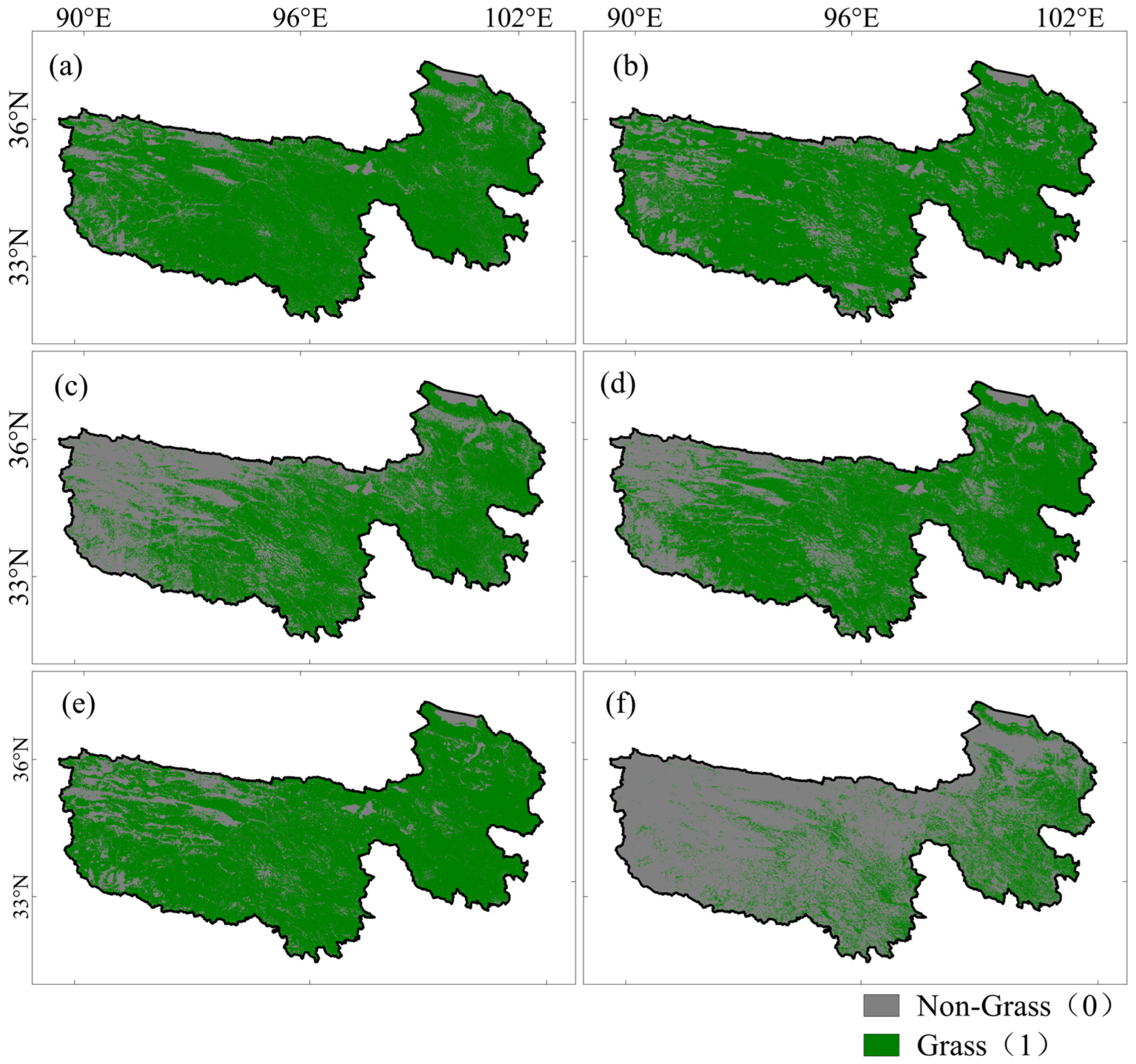
For thematic consistency, all grassland-related categories were harmonized into a single “grassland” class. Grassland pixels were assigned a value of 1, and all other land covers were assigned a value of 0, resulting in binary classification maps (Figure 2). Specifically, the ESRI product’s “Rangeland” category was considered equivalent to grassland, while in FROM_GLC10, subcategories such as “Pastures” and “Other grasslands” were merged accordingly. It should be noted that this harmonization may introduce some uncertainty, as category definitions vary across products, for example, ESRI’s “Rangeland” may include areas of shrubland or bare soil. Nonetheless, this approach provides a reasonable and practical basis for inter-product comparison.

2.2.2. Other Data

(1)

Validation Sample Data

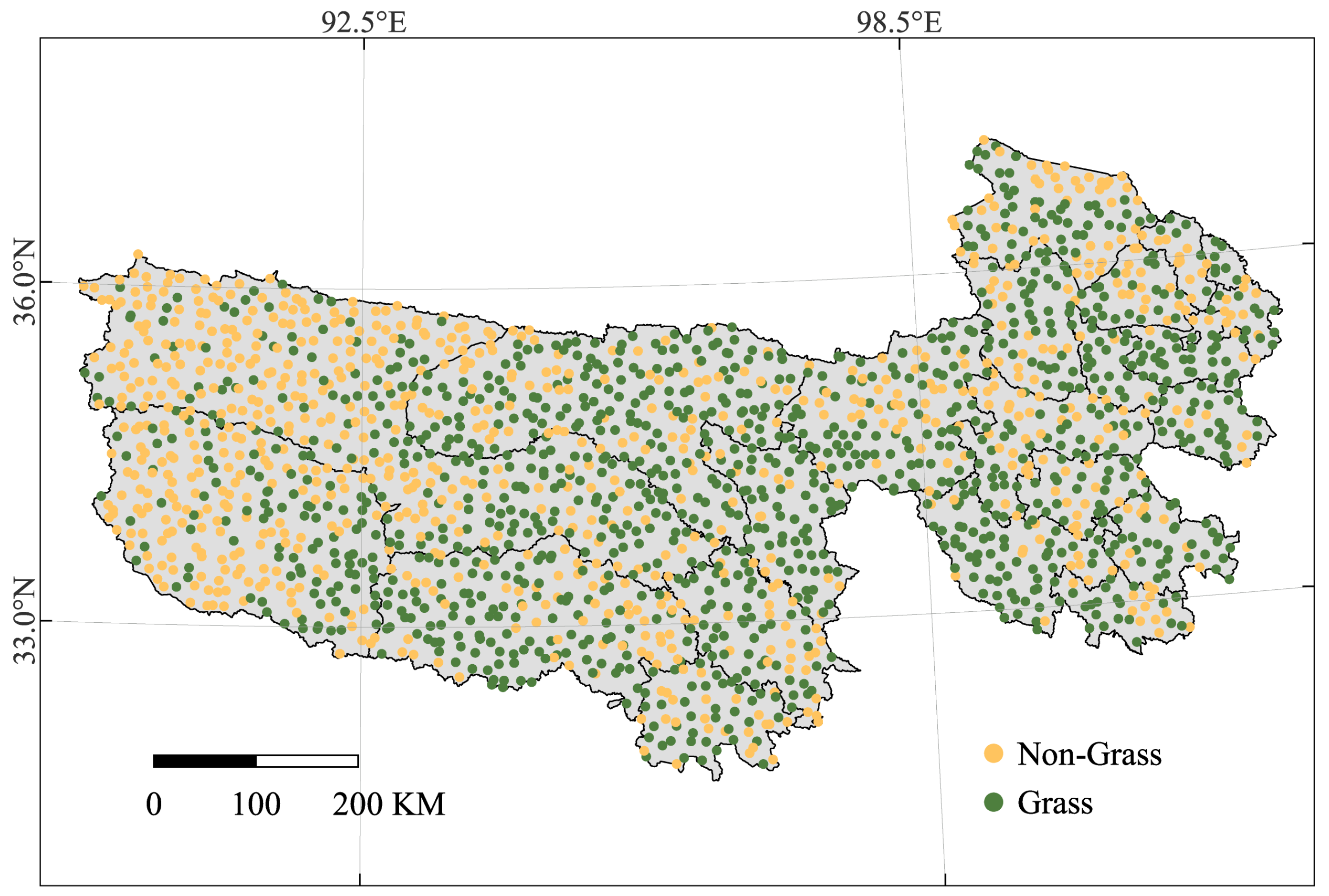
A simple random sampling strategy was adopted to generate 2007 validation points, including 1175 grassland and 832 non-grassland points (Figure 3). The sample size and distribution ensured adequate coverage of different ecological and topographic conditions in the SJYR. Sample interpretation was performed by visual analysis, with high-resolution Google Earth imagery and Gaofen-1 series 2 m resolution data serving as primary references. Additionally, multi-source auxiliary information such as vegetation indices (NDVI, NDMI) and topographic information was integrated to enhance the accuracy of sample interpretation and classification consistency.

(2)

Topographic Data

This paper introduces elevation and slope data to investigate the relationship between grassland classification results and topographic factors. The topographic data is derived from the 30 m global digital elevation model (DEM) data provided by the Shuttle Radar Topography Mission (SRTM) [47].

(3)

Grassland Area Statistics Data

This study used the Third National Land Survey of China (Third Survey) dataset from 2020 (https://gtdc.mnr.gov.cn/Share#/, accessed on 9 July 2025) as the reference for grassland area statistics. The dataset was produced using satellite imagery with spatial resolution better than 1 m as the base map, combined with extensive field surveys, mobile internet, cloud computing, UAVs, and other advanced technologies. Owing to its rigorous production process, nationwide coverage, and high thematic accuracy, this dataset serves as the most authoritative and reliable reference for validating grassland extent at the county level in the SJYR.

2.3. Methods

2.3.1. Grassland Area Statistics from Six Land Cover Products

The accurate estimation of grassland area is a fundamental prerequisite for temporal monitoring and ecological assessment. To this end, the area of “grassland” and “non-grassland” within the study region was quantified for each product, and their proportions relative to the total study area were calculated. This step reveals the overall difference in the grassland area among products.

To further validate the accuracy of the estimated grassland area for each product, this study compared the grassland area of each product with the Third Survey data at the county level. First, systematic bias was assessed through slope tests. A slope significantly deviating from 1 indicates an overall overestimation or underestimation tendency for the product. Second, the Coefficient of Determination (R²) and Root Mean Square Error (RMSE) were calculated to quantitatively evaluate the fitting quality and error levels of grassland area estimates across different counties for each product. Furthermore, to reveal the systematic bias of each product relative to the actual grassland area, the Area Difference (AD) between estimated and Third National Land Survey statistical values is calculated. This reflects the tendency of each product to overestimate or underestimate at different county scales.

$$R^2=1-{\displaystyle \frac{{\sum }_{i=1}^n(y_i-x_i{)}^2}{{\sum }_{i=1}^n(y_i-\overline{y}{)}^2}}$$

(1)

$$\mathrm{R}\mathrm{M}\mathrm{S}\mathrm{E}=\sqrt{{\displaystyle \frac{1}{n}}\sum _{i=1}^n(y_i-x_i{)}^2}$$

(2)

$${\mathrm{A}\mathrm{D}}_i={\displaystyle \frac{x_i-y_i}{y_i}}\times 100\%$$

(3)

Here, $x_i$ denotes the estimated grassland area of each product in county i; ${\mathrm{y}}_{\mathrm{i}}$ denotes the statistical grassland area of the Third Survey in county i; $\overline{\mathrm{y}}$ is the average statistical grassland area at the county level.

2.3.2. Consistency Analysis

(1)

Pairwise Consistency Analysis via the Jaccard Index

To quantify the consistency of grassland classification across different products, this study employs the Jaccard Index [48] as an evaluation metric. The Jaccard Index is a widely used tool of set similarity, defined as the ratio of the intersection to the union of two classification results. It has been extensively applied in remote sensing land–cover classification, pattern recognition, and spatial analysis [49,50,51,52], particularly suited for evaluating comparisons of binary classification results. Specifically, the six grassland classification products yield 15 pairwise combinations. For each pair, the grassland outputs are treated as binary sets, and the Jaccard Index are computed.

$$J(A,B)={\displaystyle \frac{\mid A\cap B\mid }{\mid A\cup B\mid }}$$

(4)

where A and B denote the sets of grassland pixels for two given products, $\mid A\cap B\mid$ is the area of their overlap, and $\mid A\cup B\mid$ is the area covered by either product. The index ranges from 0 to 1, with higher values indicating greater consistency between the two products in grassland identification and a higher degree of spatial overlap.

The binary grassland layers for each product pair were spatially overlaid to visualize the patterns of both their intersections and divergent areas. Additionally, a heatmap of Jaccard indices was produced to clearly illustrate the consistency differences among the six products, facilitating rapid identification of pairs with high agreement or notable divergence.

(2)

Spatial Consistency Analysis

To evaluate the spatial consistency of grassland classification among the six land cover products, we conducted a pixel-level consistency analysis. All six binary grassland maps were overlaid on a per-pixel basis, and for each pixel, we counted the number of products that classified it as grassland. Based on this count, each pixel was assigned a consistency level from 0 to 6: Level 0: No product identifies the pixel as grassland (excluded from further consideration); Levels 1–6: Correspond to 1 to 6 products, respectively, identifying the pixel as grassland. Higher levels indicate greater agreement among products and, consequently, higher confidence in grassland identification. Level 6 represents “complete agreement” across all products.

After assigning consistency levels, we calculated the total area of all pixels at Levels 1 to 6. Then we computed the consistency proportion to quantify the spatial share of each level (where i = 1, …, 6) within the grassland coverage. The consistency proportion is defined as:

$$R_i={\displaystyle \frac{N_i}{N_{\mathrm{u}\mathrm{n}\mathrm{i}\mathrm{o}\mathrm{n}}}}\times 100\mathrm{\%}$$

(5)

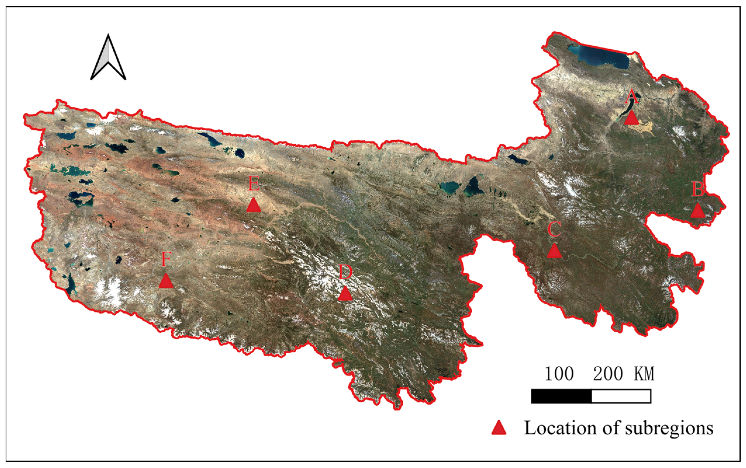
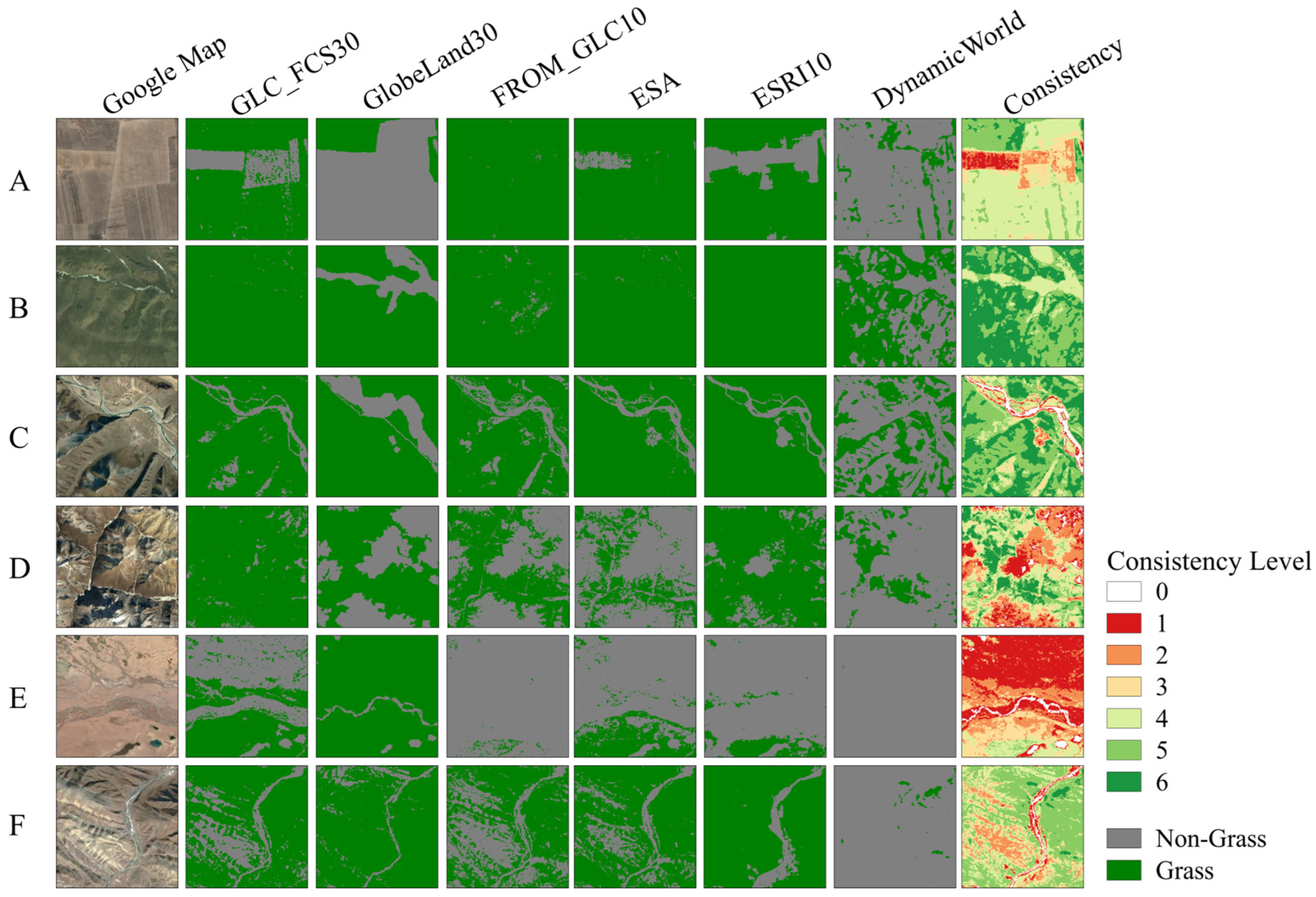
This study also selected six representative subregions, each measuring 5 km × 5 km, within the study area (Figure 4) for comparative analysis. These areas encompass typical diverse ecological environments characteristic of the SJYR, including relatively flat meadow zones with high vegetation cover, transitional zones where grasslands intermingle with other land types, rugged alpine canyon areas, and arid zones dominated by sparse grasslands and bare ground. By comparing the classification results and consistency levels of each product under varying natural conditions, this study reveals the adaptability and performance differences of different products across complex environmental gradients.

2.3.3. Confusion Matrix and Accuracy Assessment

To assess the classification performance of each product, we employed a binary confusion matrix [53], treating “grassland” as the positive class and “non-grassland” as the negative class.

• True Positive (TP): actually grassland and predicted as grassland;
• False Positive (FP): actually non-grassland and predicted as grassland;
• True Negative (TN): actually non-grassland and predicted as non-grassland;
• False Negative (FN): actually grassland and predicted as non-grassland.

From this confusion matrix, we calculated five accuracy metrics, including overall accuracy (OA), producer’s accuracy (PA), user’s accuracy (UA), F1 score, and the Matthews correlation coefficient (MCC). OA is defined as the proportion of all correctly classified pixels to the total number of validation samples. PA is a metric that quantifies omission error for the grassland class, defined as the proportion of reference grassland pixels that are correctly mapped as grassland. UA measures commission error for grassland, defined as the proportion of pixels labeled as grassland that are truly grassland, thereby reflecting misclassification into this class. The F1 score is the harmonic mean of PA and UA, balancing omission and commission errors to provide a consolidated measure of grassland detection performance. The MCC incorporates TP, TN, FP, and FN into a single correlation coefficient, offering a statistically robust assessment of classification quality. The formulas are as follows:

$$\mathrm{O}\mathrm{A}={\displaystyle \frac{TP+TN}{TP+TN+FP+FN}}$$

(6)

$$\mathrm{P}\mathrm{A}={\displaystyle \frac{TP}{TP+FN}}$$

(7)

$$\mathrm{U}\mathrm{A}={\displaystyle \frac{TP}{TP+FP}}$$

(8)

$$F_1=2\times {\displaystyle \frac{\mathrm{P}\mathrm{A}\times \mathrm{U}\mathrm{A}}{\mathrm{P}\mathrm{A}+\mathrm{U}\mathrm{A}}}$$

(9)

$$\mathrm{M}\mathrm{C}\mathrm{C}={\displaystyle \frac{TP\times TN-FP\times FN}{\sqrt{(TP+FP)\hspace{0.17em}(TP+FN)\hspace{0.17em}(TN+FP)\hspace{0.17em}(TN+FN)}}}$$

(10)

3. Results

3.1. Analysis of Six Land Cover Products Based on Area

In terms of grassland area, the six land cover products show significant differences in identification results within the study area (

Table 3. Grassland area (km²) and proportion (%) derived from six land cover products in the SJYR.

	GLC_FCS30	GlobeLand30	FROM_GLC10	ESA	ESRI	Dynamic World
Area (km2)	325,669.28	311,595.22	227,187.42	269,262.43	322,775.5	91,105.19
Proportion (%)	87.09	80.16	58.45	69.27	83.04	23.44

). GLC_FCS30 and ESRI products report the highest and second-highest grassland area, at 325,669.28 km² and 322,775.50 km², respectively, accounting for 87.09% and 83.04% of the study area; GlobeLand30 follows closely, with grassland areas of 311,595.22 km² and a proportion of 80.16%. In contrast, FROM_GLC10 and ESA are more conservative in their grassland estimates, at 227,187.42 km² (58.45%) and 269,262.43 km² (69.27%), respectively. Dynamic World, significantly underestimates grassland areas compared to other products, estimating only 91,105.19 km² of grassland, which accounts for 23.44% of the total.

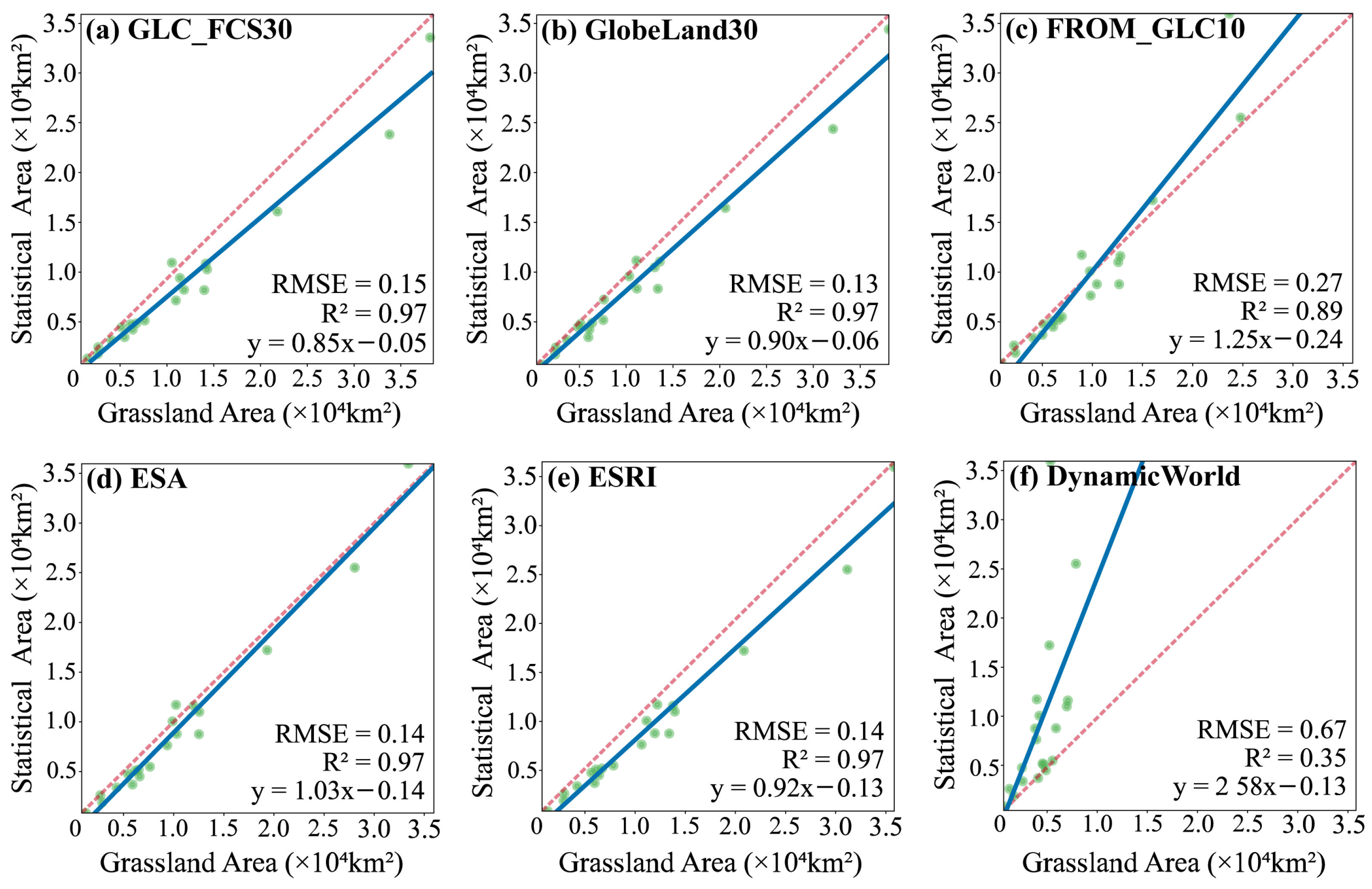
This study conducted a regression analysis of the correlation between six land cover products and the “Third Survey” data (Figure 5). The results indicate that ESA exhibits the closest regression slope to 1 (slope = 1.03), with an R2 of 0.97 and RMSE of 0.14 × 10⁴ km², also demonstrating excellent performance. Both GlobeLand30 and GLC_FCS30 exhibited slopes below 1, indicating overall overestimation. However, both models demonstrated high fit quality and maintained strong consistency with statistical data. ESRI showed relatively weaker performance: although its R2 (0.97) and RMSE (0.14 × 10⁴ km²) were satisfactory, its stability and consistency were slightly inferior to those of the other two models. In contrast, FROM_GLC10 exhibits poor fit (R2 = 0.89, RMSE = 0.27 × 10⁴ km²) with a slope of 1.25, indicating significant underestimation; Dynamic World performed worst with R2 = 0.35 and RMSE = 0.14 × 10⁴ km², exhibiting the most severe underestimation among all products.

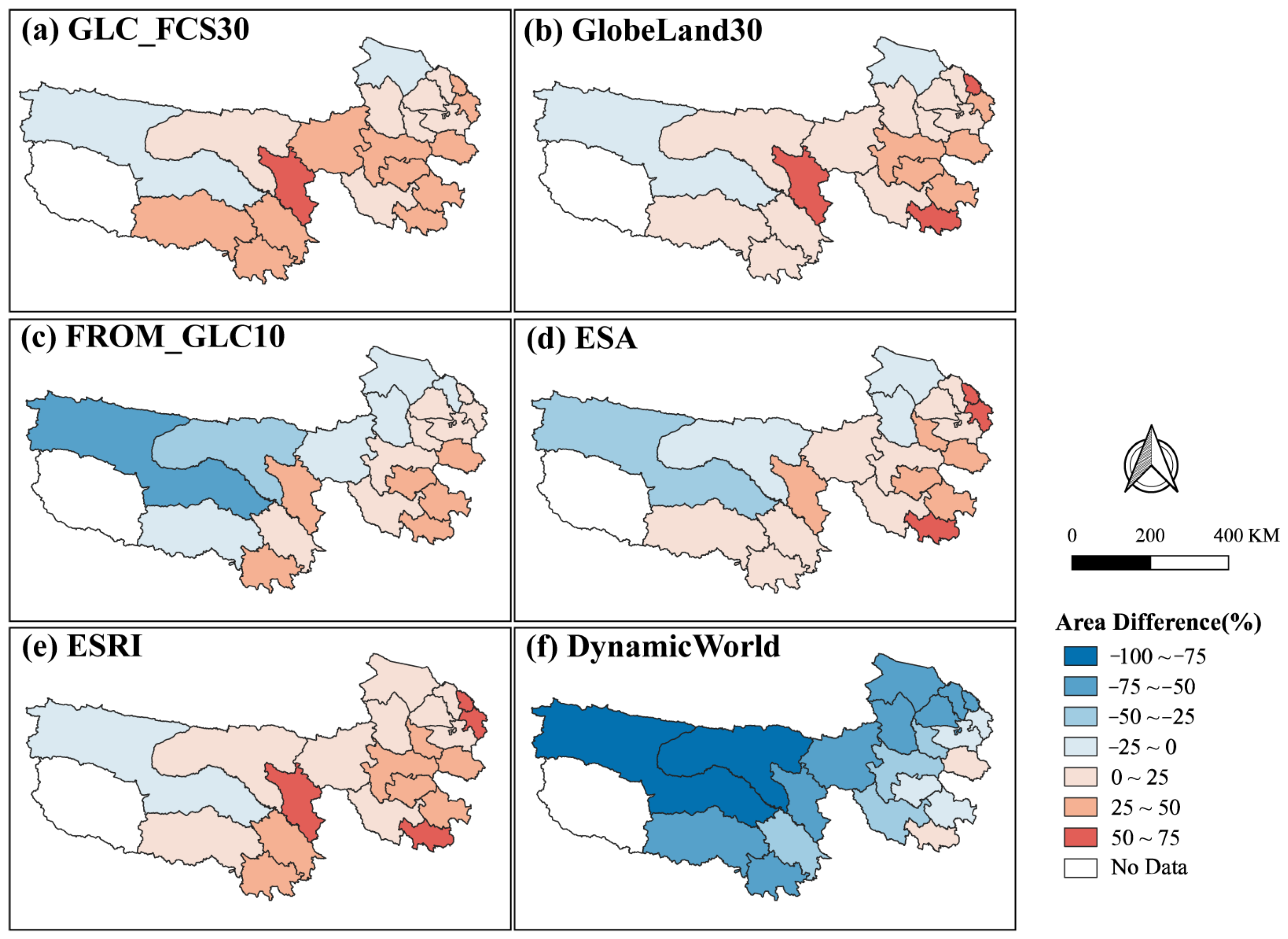
Figure 6 shows the spatial distribution of AD among various products at the county administrative level. Overall, all products generally exhibit a pattern of overestimation in the eastern and central regions and underestimation in western counties. Specifically, GLC_FCS30, GlobeLand30, and ESRI all show a relatively evident tendency toward overestimation, with AD exceeding 50% in some eastern counties; ESA exhibits a relatively stable performance, although it also shows a trend of overestimation in the eastern regions and underestimation in the western regions, the magnitude of the deviation is minor. FROM_GLC10 has the lowest average deviation, while underestimation in western counties (such as Zhiduo County) can reach −50%. Dynamic World severely underestimates in the vast majority of counties, with AD below −75%.

3.2. Pairwise Consistency of Six Products

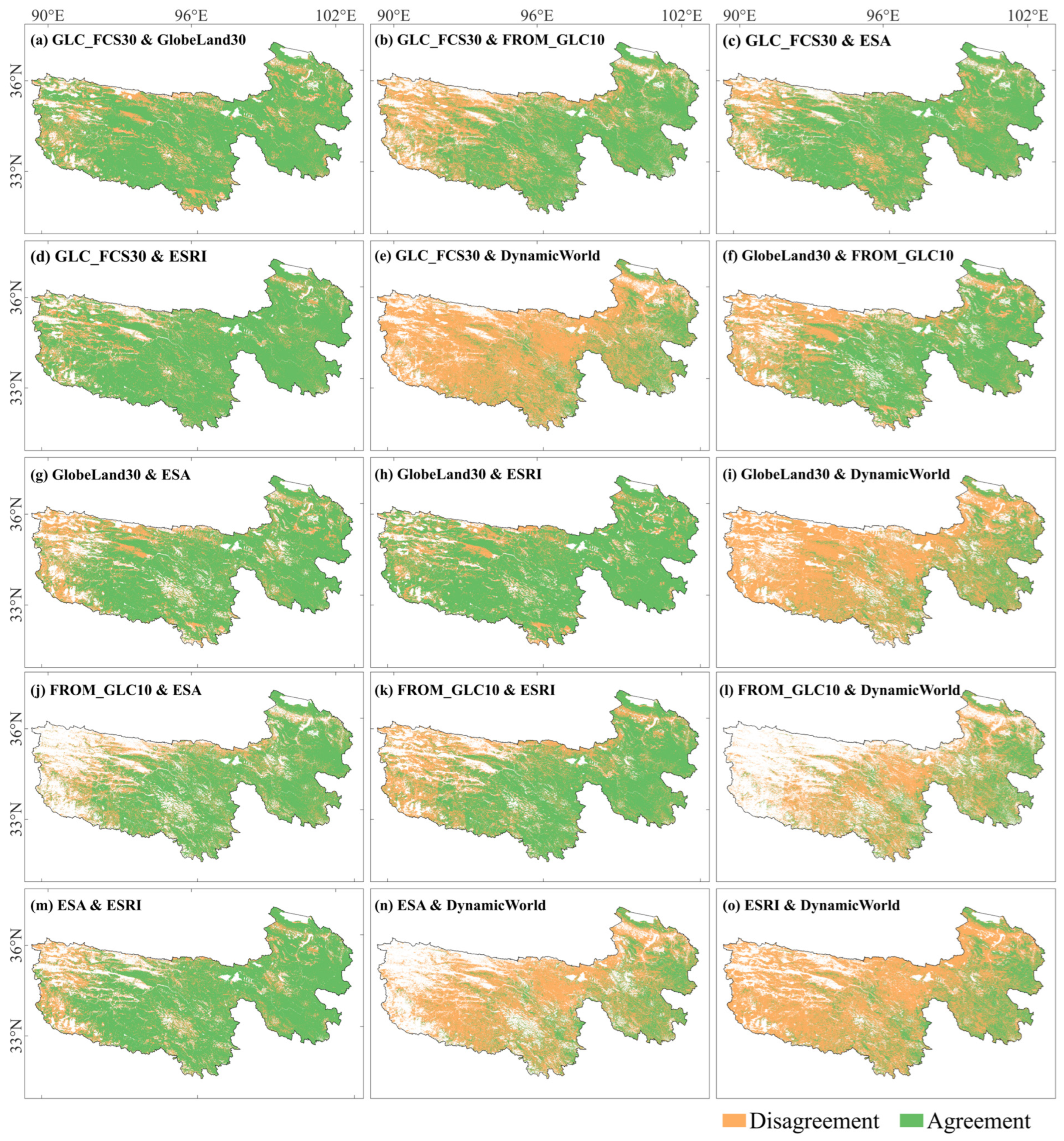
Figure 7 shows the spatial distribution patterns of the pairwise overlaps in grassland classification among the six land cover products. From a quantitative perspective, the overall area percentage of agreement for all product pairs is comprehensively presented by the Jaccard similarity coefficients heatmap in Figure 8. From a spatial distribution perspective, higher agreement is observed in the eastern part of the study area, where the overlapping regions of grassland classification are extensive and the consistency among products is relatively high. In contrast, the western region exhibits greater divergence, with a significantly larger extent of non-overlapping areas, indicating pronounced spatial heterogeneity in grassland classification results.

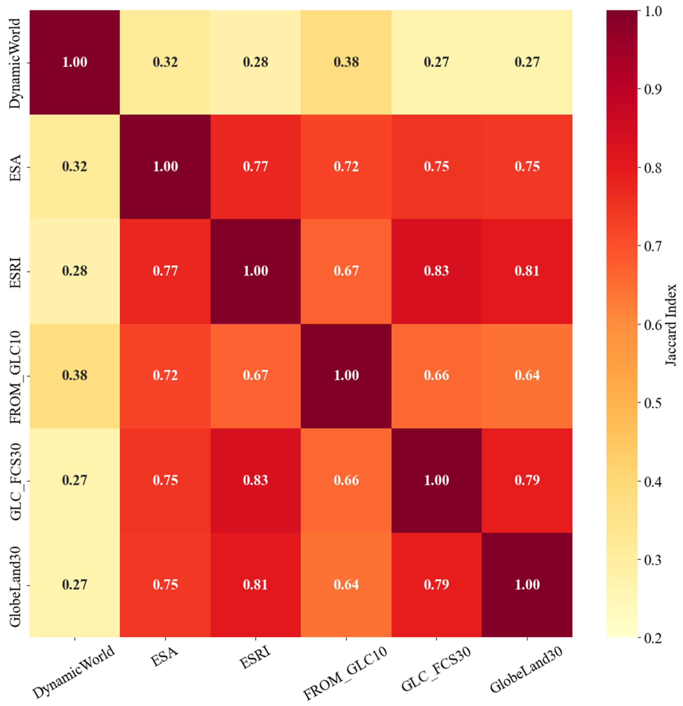
Figure 8 quantitatively assesses the pairwise consistency of six products in grassland classification, reflecting the spatial overlap of grassland categories among products. Results indicate that Dynamic World exhibits significantly lower Jaccard coefficients compared to the other five products: 0.28 with ESRI, 0.27 with GLC_FCS30, and 0.27 with GlobeLand30. This suggests limited spatial consistency in grassland distribution between Dynamic World and other products. In contrast, the remaining five products demonstrate higher mutual consistency, with coefficients generally ranging from 0.66 to 0.83. with the highest spatial consistency observed between ESRI and GLC_FCS30 (0.83), followed by ESRI and GlobeLand30 (0.81), GLC_FCS30 and GlobeLand30 (0.79), and ESA and ESRI (0.77). FROM_GLC10 exhibits moderate similarity with other products (e.g., 0.72 with ESA, 0.67 with ESRI, 0.66 with GLC_FCS30, and 0.69 with GlobeLand30), suggesting that while it remains broadly comparable to the major datasets, its overall consistency is lower than that observed among products derived from the same temporal baseline.

3.3. Grassland Spatial Consistency of Six Products

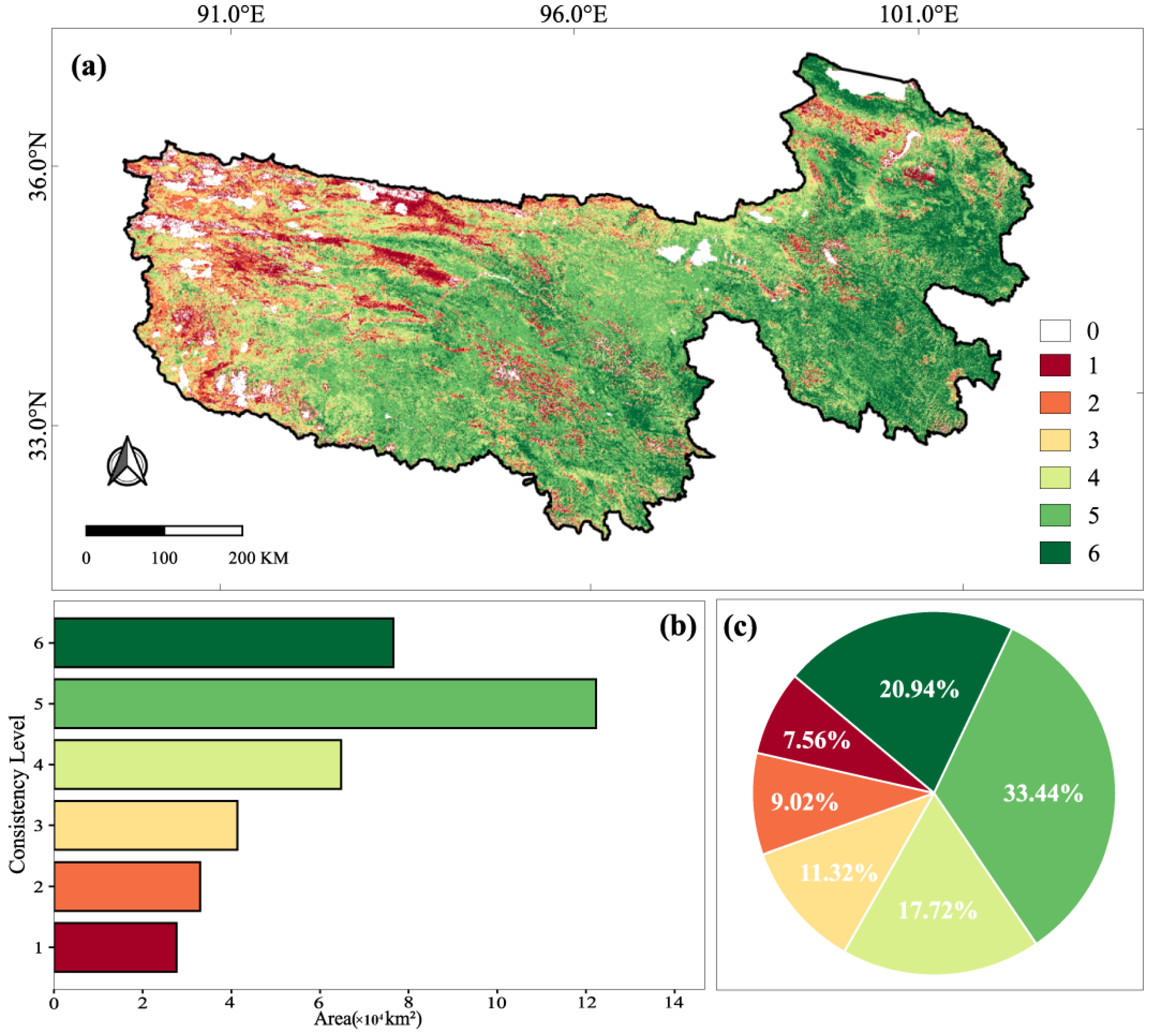
Based on the pixel-level spatial consistency grading approach, a spatial consistency map of grassland classification was generated. Figure 9a shows the spatial distribution patterns of each consistency level across the study area, revealing a clear contrast between the eastern and western regions, with significantly higher consistency observed in the east. This study calculated the area and proportion of regions with different consistency levels, as shown in Figure 9b,c. Among the six products, the total area of high consistency level regions (Levels 5 and 6) was 19.88 × 10⁴ km², accounting for 54.3% of the total study area. Levels 5 and 6 covered 12.23 × 10⁴ km² (33.4%) and 7.66 × 10⁴ km² (20.9%), respectively. This indicates that the results of grassland classification are consistent across more than half of the study area. The total area of regions with moderate consistency levels (Levels 3 and 4) is 10.61 × 10⁴ km², accounting for 29.5%, indicating that there is still uncertainty in grassland classification in some areas. The total area of low consistency level regions (Levels 1 and 2) is 6.02 × 10⁴ km², accounting for 16.2%, with the lowest consistency level (Level 1) regions covering 27,664.57 km² (7.4%) and Level 2 regions covering 32,567.50 km² (8.8%). These regions are primarily concentrated along grassland boundaries, transition zones, and complex terrain regions, representing the regions with the most significant classification discrepancies.

This study selected six representative typical zones and compared the grassland classification results and consistency levels of each product at the same spatial scale (Figure 10). Specifically, A is an agricultural-pastoral transition zone with gentle topography, featuring a mix of cropland and grassland. All six products exhibit mixed classifications of cropland and grassland, but GLC_FCS30 and GlobeLand30 display relatively smoother and more continuous boundaries. In contrast, some 10 m-resolution products, while offering higher resolution, exhibit fragmented boundaries due to their heightened sensitivity to small-scale heterogeneity. B is located in the humid meadows area of the southeastern part of the study area, characterized by high vegetation coverage continuity, relatively uniform vegetation, and a stable ecological environment. Classification results for various products in this area show minimal variation, demonstrating overall high consistency. C is located in the river floodplain grassland zone. GLC_FCS30, ESA, and ESRI demonstrate relatively accurate patch identification, while Dynamic World exhibits misclassification in specific patches. Red areas (Levels 1 and 2) primarily correspond to riverbank bare land and rocky beaches, and minor misclassifications occur around impervious surfaces (such as roads and scattered settlements) across all products. D is a mountainous area with alpine steppes, characterized by rugged terrain and complex ecological patches. Spatial consistency heterogeneity is generally at Levels 2 to 4, and consistency exhibits significant instability in such regions. E is located in the western desert region of the study area, with sparse grasslands and bare land interspersed. Most products classify this region as non-grassland, with only a few patches labeled as grassland. In the consistency map, over 75% of the area is classified as level 0 or 1. F is a canyon area with vegetation distributed in bands. GLC_FCS30, FROM_GLC10, and ESA accurately identify the boundary between bare land and grassland, while GlobeLand30 and ESRI exhibit overestimation.

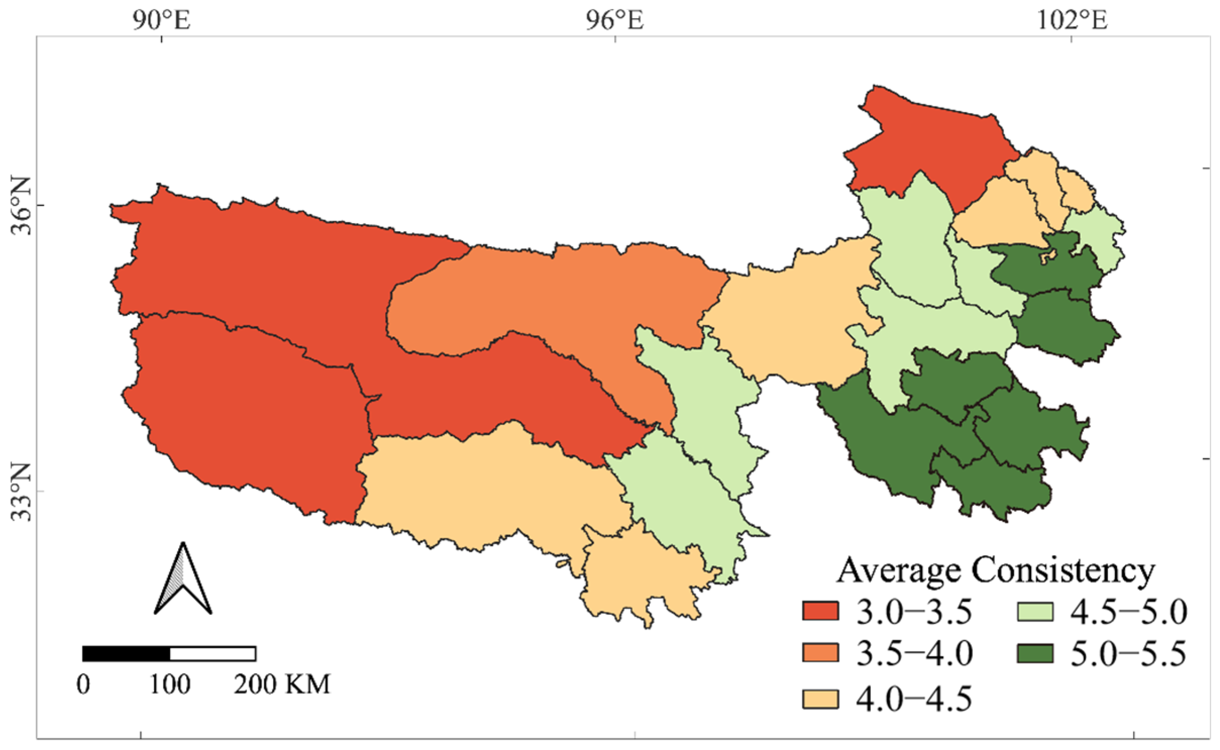
While pixel-level consistency reveals fine-scale spatial heterogeneity, county-level aggregation provides a complementary administrative-unit perspective that is useful for identifying broader regional patterns and supporting ecological management decisions in the SJYR. Therefore, we additionally summarized consistency at the county scale to highlight cross-county variation that is not directly observable from pixel-based maps. As shown in Figure 11, the consistency of grassland classification varies considerably among counties, exhibiting a distinct spatial differentiation pattern. Specifically, the southeastern counties, including Gande, Dari, Jiuzhi, Banma, Zeku, and Henan, show higher levels of consistency, with average values exceeding 5.0. This indicates that the classification results from different land cover products in these areas are relatively consistent, reflecting high spatial agreement and strong classification stability. In contrast, the western counties, such as Zhiduo and Golmud, exhibit significantly lower consistency levels, with average values below 3.5.

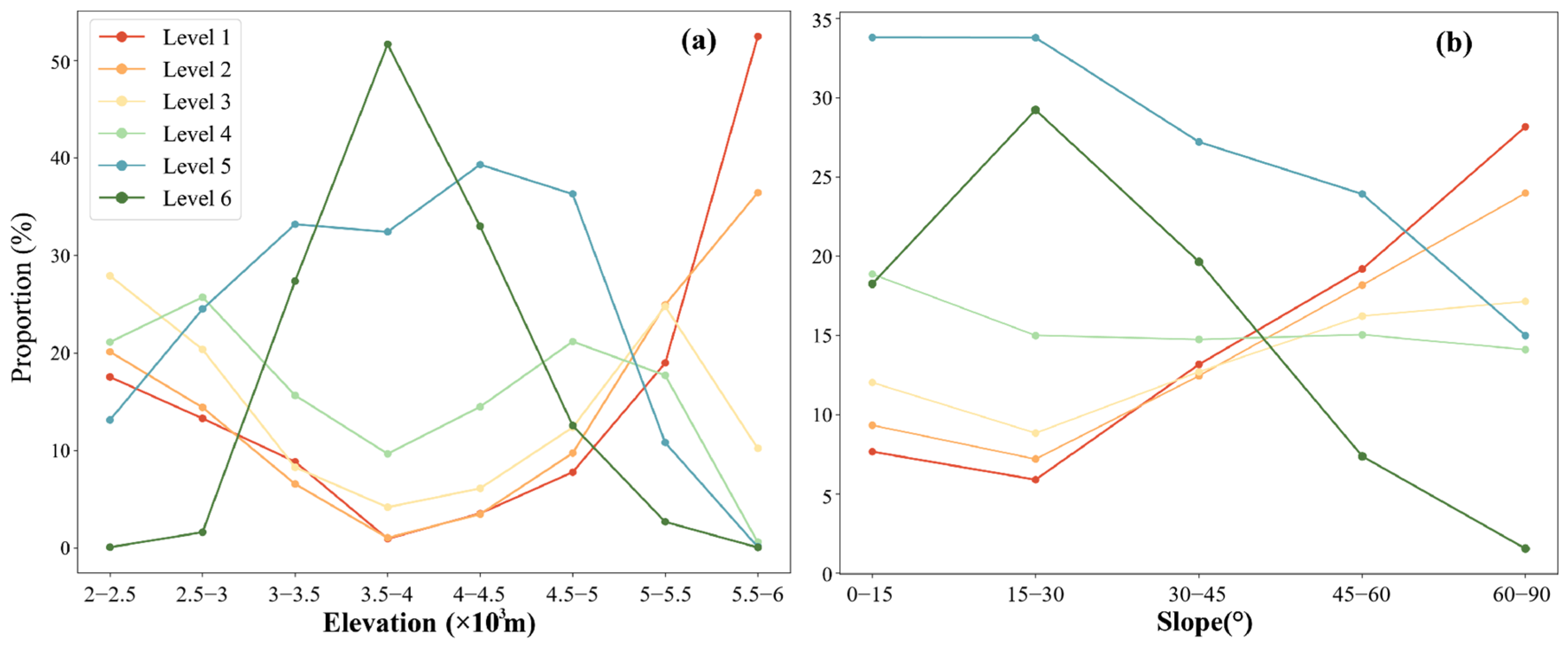
To further investigate the influence of topographic factors on the spatial consistency of grassland classification, a stratified statistical analysis was conducted for the SJYR. The proportion of each consistency level under varying topographic conditions was calculated, as shown in Figure 12. The results indicate that topography has a significant impact on classification consistency. In terms of elevation, the 3500–4000 m range exhibits the highest consistency, with high-consistency levels (Levels 5 and 6) accounting for over 80% of the area, and low-consistency levels (Levels 1 and 2) showing the lowest proportions. This suggests that remote sensing products tend to yield more consistent grassland classification results within this elevation range. However, as elevation increases, the proportion of high-consistency areas declines sharply. In regions above 4500 m, the share of high-consistency classifications drops dramatically, while the proportion of low-consistency levels rises significantly. Furthermore, a similar pattern is observed for slope. High-consistency classifications are predominantly found in areas with slopes less than 30°. As the slope increases, the proportion of high-consistency levels gradually decreases, while that of low-consistency levels continues to rise. Notably, in areas with slopes greater than 30°, the share of low-consistency classifications (Levels 1 and 2) increases rapidly. These findings underscore the critical role of topographic factors in influencing the spatial consistency of remote sensing-based grassland classification.

3.4. Grassland Classification Accuracy of Six Products

3.4.1. Accuracy Comparison of Six Products for Grassland in the SJYR

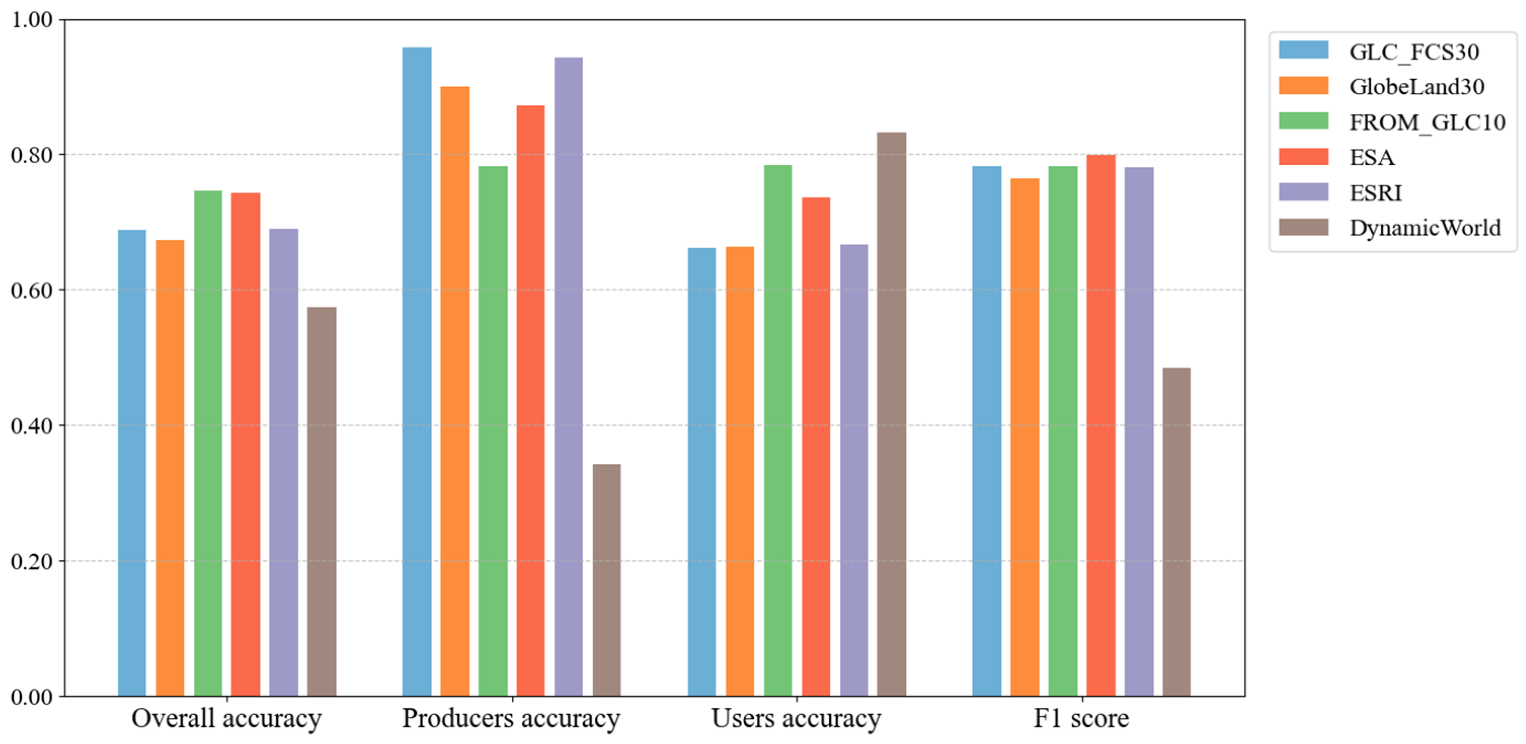
The accuracy analysis results (

Table 4. Accuracy metrics (OA, PA, UA, F1-score, and MCC) for grassland classification across six products in the SJYR.

	OA	PA	UA	F1	MCC
GLC_FCS30	68.81%	95.74%	66.14%	0.78	0.36
GlobeLand30	67.41%	89.96%	66.35%	0.76	0.31
FROM_GLC10	74.64%	78.21%	78.41%	0.78	0.48
ESA	74.24%	87.15%	73.67%	0.80	0.46
ESRI	69.01%	94.21%	66.65%	0.78	0.36
Dynamic World	57.45%	34.21%	83.23%	0.48	0.28

and Figure 13) indicate that FROM_GLC10 and ESA exhibit high overall accuracy (OA) values of 74.64% and 74.24%, respectively. ESRI, GLC_FCS30, and GlobeLand30 achieved OA values of 69.01%, 68.81%, and 67.41%, respectively. Dynamic World demonstrated the lowest OA at only 57.45%. In terms of specific metrics, ESA demonstrates greater balance (F1 = 0.80), indicating stronger stability in reducing both false negatives and false positives. FROM_GLC10 exhibits a relatively low Precision (PA) of 78.21%, suggesting significant underclassification of grassland areas, leading to an overall underestimation of grassland coverage. GLC_FCS30 (PA = 95.74%) and ESRI (PA = 94.21%) exhibit high PA but low UA (66.14% and 66.65%, respectively), revealing a tendency for false positives—misclassifying non-grassland as grassland, resulting in overestimation of area. GlobeLand30 exhibits similar behavior (PA = 89.96%, UA = 66.35%). Dynamic World achieved 83.23% in UA, the highest among all products, indicating that most of its predicted grassland areas were actual grasslands. However, its PA was only 34.21%, revealing that it missed many points and failed to identify a large number of actual grasslands, resulting in incomplete classification results. The MCC metric further validates this trend. This metric comprehensively evaluates the correlation between TP, TN, FP, and FN, with higher values indicating classification results closer to the true distribution. Results show FROM_GLC10 (MCC = 0.48) and ESA (MCC = 0.46) achieved the highest scores, indicating strong alignment with actual distribution. Conversely, Dynamic World (0.28) exhibits lower MCC, reflecting insufficient classification stability.

3.4.2. Accuracy Comparison of Grassland in Different Topographical Conditions

The previous study [39] and the spatial consistency analysis described earlier in this paper both indicate that topography has a significant impact on grassland classification results. To further quantify this effect, this study compared the classification accuracy of various products under different topographic conditions (Figure 14).

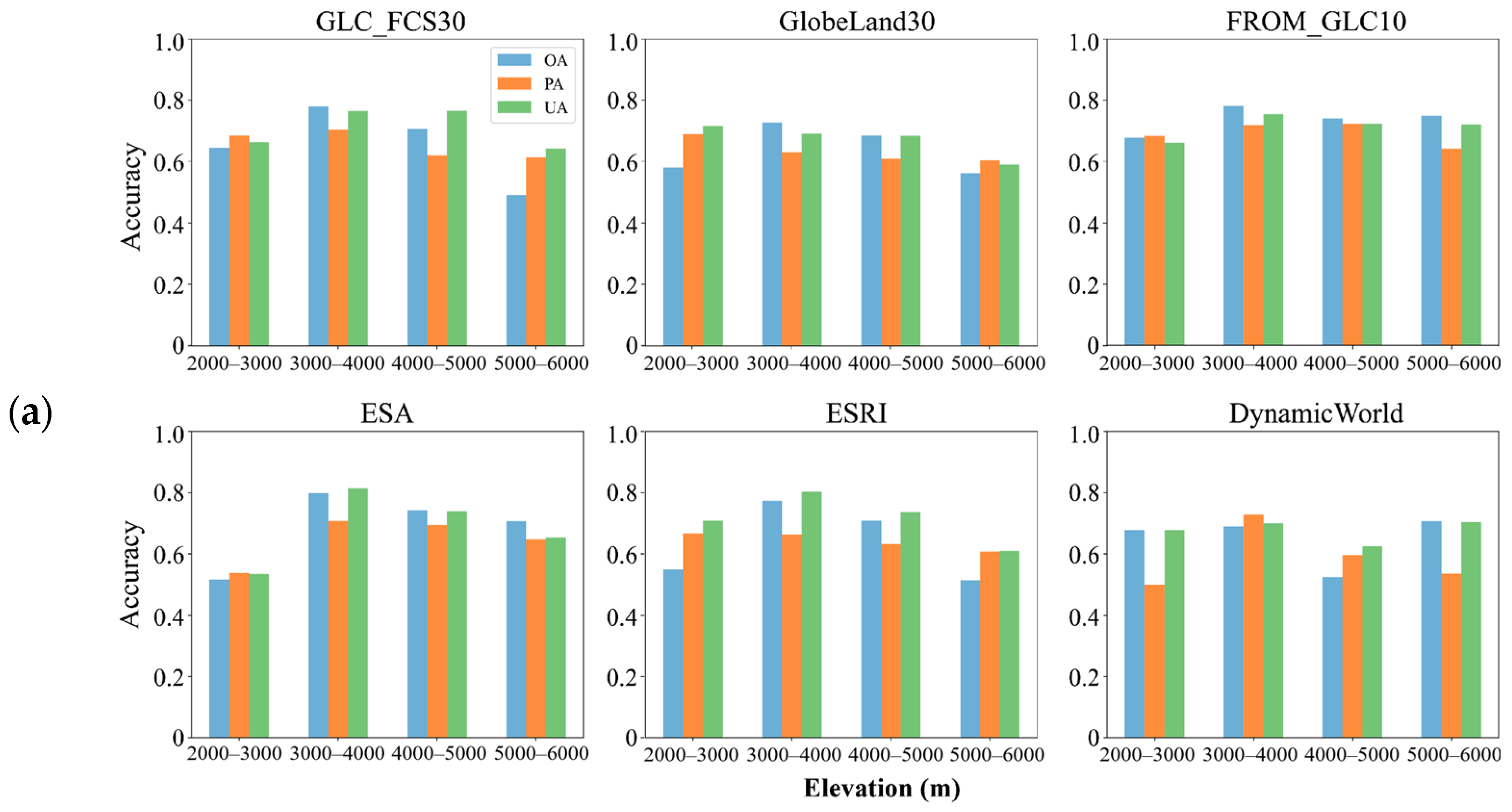
Figure 14a demonstrates varying performance across different elevation ranges. Most products exhibit optimal classification performance within the 3000–4000 m elevation range. As altitude increases, the classification accuracy of most products decreases, especially in high-altitude regions above 5000 m, where the OA of ESA, ESRI and GLC_FCS30 all drop below 0.70, indicating a significant decline in accuracy.

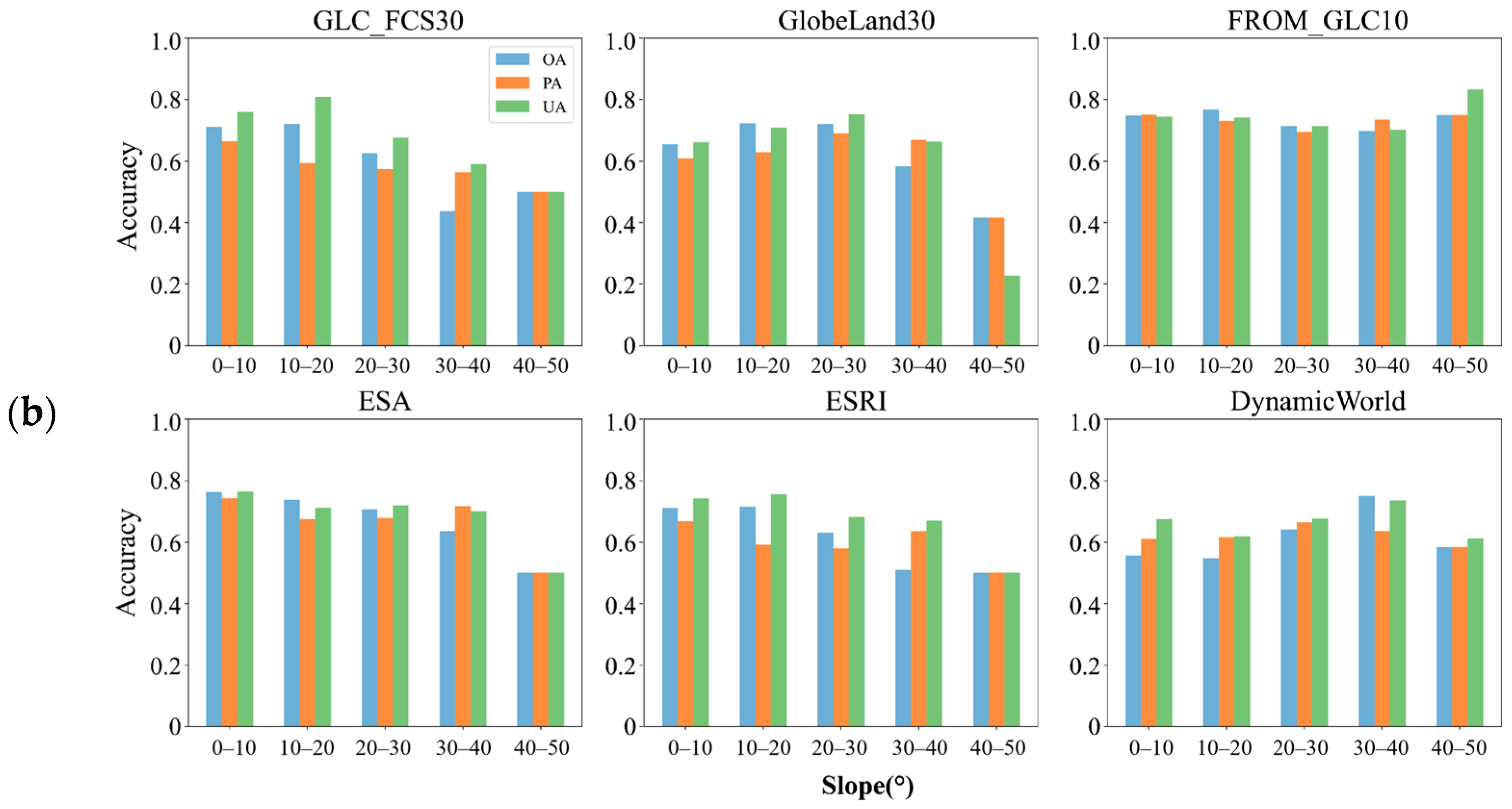
In terms of slope, the study categorizes it into five grades: 0–10°, 10–20°, 20–30°, 30–40°, and 40–50°. Since areas with slopes exceeding 50° have a tiny coverage area and a limited sample size, they were not included in the analysis. As shown in Figure 14b, in low-slope areas (0–20°), all products exhibit high precision and demonstrate consistent performance across all metrics. In the 20–30° slope range, FROM_GLC10 and ESA maintain PA and UA values above 0.7, indicating better resilience to topographic variability. However, the OA of ESRI and GLC_FCS30 drops to 0.63, indicating a decline in classification accuracy. As the slope increases, the accuracy of most products further decreases, exhibiting strong terrain dependency, particularly for ESRI and GLC_FCS30. Notably, despite Dynamic World’s overall lower accuracy, its OA variation remains relatively stable across different slope intervals (maintaining around 0.60), indicating a certain degree of resistance to terrain changes. This stability may be attributed to the product’s high rate of underclassification, meaning that while it may fail to identify specific features, it also makes fewer misclassifications, thereby maintaining a low but relatively constant accuracy level across different terrains.

4. Discussion

4.1. Summary of Findings

This study provides a comprehensive assessment of grassland classification consistency and accuracy across six widely used global land cover products—GLC_FCS30, GlobeLand30, FROM_GLC10, ESA, ESRI, and Dynamic World—within the SJYR, one of the most ecologically sensitive and topographically complex areas of the Qinghai–Tibet Plateau.

The six products exhibit significant differences in both area estimation and spatial distribution. For instance, GLC_FCS30 identified a massive grassland area (325,669.28 km²), contrasting sharply with the Dynamic World product (only 91,105.19 km²). Spatial overlay analysis revealed that the eastern part of the SJYR exhibited relatively high spatial consistency in grassland identification across products, whereas the western part showed significant discrepancies, with a noticeable increase in the extent of inconsistent areas. Overall, ESA generally exhibiting higher agreement and more stable performance across metrics (OA = 74.24%, MCC = 0.80),while Dynamic World exhibited the weakest spatial consistency the lowest levels of and accuracy (OA = 57.45%, F1 = 0.28) among the six products.

The study also confirmed a correlation between classification consistency and topographic factors. Differences among products were most pronounced in high-elevation and steep-slope areas. Specifically, we found a noticeable decline in product precision at elevations above 4000 m and on slopes steeper than 10°. This quantitative evidence indicates that remote-sensing-based classification faces significantly higher uncertainty under these complex terrain conditions. Previous studies have also demonstrated classification uncertainty in topographically heterogeneous areas [54,55], indicating that improving classification accuracy in such regions remains a significant challenge.

4.2. Factors of the Uncertainty in Grassland Classification Results

According to the evaluation results of this study, the six products exhibited significant differences in grassland area, spatial consistency, and accuracy performance, reflecting the uncertainty of current global land cover products in grassland identification within alpine ecological zones. However, the source of uncertainty among these products is complex, and a combination of factors leads to significant differences in the grassland identification results of different products in the same region. In order to deeply understand the causes of these differences, the study analyses them from the following aspects.

4.2.1. Differences in Remote Sensing Data Sources

Due to the differing remote sensing data sources for the six products, systematic differences in classification performance are observed. For example, GLC_FCS30 and GlobeLand30 primarily use Landsat series imagery (30 m resolution) as their foundation, while FROM_GLC10, ESA, ESRI, and Dynamic World utilize higher-resolution Sentinel-2 data (10 m). ESA also integrates Sentinel-1 radar data. High-resolution imagery provides a more detailed representation of landform internal details and texture features [37], aiding in the identification of patch boundaries and small-scale heterogeneous landscapes [45]. However, increased resolution also introduces more noise into the classification process. Additionally, differences in spectral bandwidth and centre wavelengths among sensors affect the calculation of vegetation indices and texture features, thereby influencing grassland classification outcomes [56]. Furthermore, the complex terrain undulations and local cloud cover in the SJYR impose higher requirements on sensor signal-to-noise ratio, band selection, and imaging timing. These factors collectively contribute to the inconsistency in grassland classification results across different products.

4.2.2. Differences in Classification Methods and Classification Systems

Different classification methods and classification systems were adopted for each product (see Section 2.2.1). Deep learning models can utilize contextual information around pixels during classification, whereas traditional random forest methods primarily rely on the features of the pixels themselves [45]. This difference directly impacts their adaptability to complex terrain or small-scale landscapes, resulting in varying robustness when handling mixed pixels, slope shadows, and small-scale patches. In addition, different products have inconsistent definitions of the grassland category, and differences in these definitions in key elements can also lead to differences in classification results [25,57]. For example, ESRI classifies grassland categories under “Rangeland”, which encompasses not only natural grasslands but may also include patches of shrubland and bare ground, contributing to uncertainty when comparing it with other datasets. GLC_FCS30 applies a relatively strict definition (vegetation cover ≥ 15%), its results still exhibit an obvious overestimation of grassland area in the SJYR. This suggests that factors may have contributed to reduced classification accuracy. This bias is likely driven by the coarser 30 m spatial resolution, which is more susceptible to mixed-pixel effects in the sparsely vegetated and heterogeneous alpine landscape of the SJYR. In particular, the patchy vegetation structure, strong bare-soil background signals, and terrain-induced spectral variability reduce the separability between grassland and non-grassland classes, collectively contributing to the overestimation observed in GLC_FCS30.

4.2.3. Differences in Temporal Reference

Both species characteristics and climate change influence the phenology of grasslands. The growing seasons of different grassland types vary, and may change annually due to fluctuations in precipitation and temperature [58]. In the SJYR, the grassland growing season is short [59], and grassland ecology is highly sensitive to seasonal precipitation, livestock grazing, and freeze-thaw cycles [10,60]. The coverage and spectral characteristics of grasslands may vary across different years and growing seasons [61]. Since different land cover products use images captured on different dates, land cover at the exact location may change, leading to discrepancies in classification results. It should also be emphasized that differences in the reference years among products (e.g., FROM_GLC10 based on 2017 imagery vs. other products based on 2020) may partially contribute to the observed inconsistencies. Although this temporal effect could not be fully quantified in this study, it remains one source of uncertainty.

4.3. Recommendations for Future Grassland Research

Firstly, due to the extremely large geographic extent, harsh climatic conditions, and limited accessibility of the SJYR, comprehensive field-based surveys were not feasible during this study. Although high-resolution Google Earth and Gaofen-1 imagery provided reliable visual references for building the validation dataset, the lack of field observations remains a limitation. Field-based data would further enhance the reliability of grassland type identification, particularly in areas with highly heterogeneous terrain [62]. Therefore, future research should incorporate partial field sampling in ecologically sensitive or topographically complex regions, supported by UAV imagery or semi-automatic labeling tools, to improve the spatial coverage and representativeness of ground-truth samples.

Secondly, the accuracy and robustness of grassland classification can be improved by integrating multiple products through multi-source product fusion or integrated learning methods. For example, the grassland classification results of different products can be fused through weighted or voting mechanisms [63] to reduce the error caused by noise from a single product. Liu et al. [64] fused multiple land cover products based on the improved Dempster-Shafer evidence theory, achieving an accuracy of 85.32% in Central Asia, which is higher than the accuracy of individual products.

Thirdly, most current products treat “grassland” as a single category, lacking a fine-grained expression of grassland classification. The SJYR has an urgent need for fine-grained monitoring of grasslands [59]. Based on existing high-precision field survey data and drone aerial imagery, a high-altitude grassland subcategory annotation database can be constructed, further subdivided into ecological types such as alpine meadows, alpine grasslands, and sparse grasslands. By integrating spectral data, vegetation indices, texture, topography, and climate characteristics, multi-level classification modelling can be conducted to achieve precise monitoring and scientific management of complex alpine grasslands.

5. Conclusions

This study systematically evaluated the spatial consistency and accuracy of six global land cover products (GLC_FCS30, GlobeLand30, FROM_GLC10, ESA, ESRI and Dynamic World) in grassland classification over the SJYR. The findings highlight substantial differences in grassland area estimation and spatial patterns, with ESA showing relatively reliable performance, while Dynamic World significantly underestimates grassland extent. Pixel-level analysis reveals that regions with complex terrain, particularly the western high mountains, exhibit the greatest disagreement across products, underscoring the role of topography in classification uncertainty. These results emphasize the need for improved algorithms and multi-source data integration tailored to alpine environments and provide a scientific basis for selecting appropriate land cover products for ecological monitoring and grassland management in the SJYR.

References

1. Blair, J.; Nippert, J.; Briggs, J. Grassland Ecology. In Ecology and the Environment; Monson, R.K., Ed.; Springer: New York, NY, USA, 2013; pp. 1–30. ISBN 978-1-4614-7612-2. [Google Scholar]
2. Bengtsson, J.; Bullock, J.M.; Egoh, B.; Everson, C.; Everson, T.; O’Connor, T.; O’Farrell, P.J.; Smith, H.G.; Lindborg, R. Grasslands—More Important for Ecosystem Services than You Might Think. Ecosphere 2019, 10, e02582. [Google Scholar] [CrossRef]
3. Chang, J.; Ciais, P.; Gasser, T.; Smith, P.; Herrero, M.; Havlík, P.; Obersteiner, M.; Guenet, B.; Goll, D.S.; Li, W.; et al. Climate Warming from Managed Grasslands Cancels the Cooling Effect of Carbon Sinks in Sparsely Grazed and Natural Grasslands. Nat. Commun. 2021, 12, 118. [Google Scholar] [CrossRef] [PubMed]
4. Scholtz, R.; Twidwell, D. The Last Continuous Grasslands on Earth: Identification and Conservation Importance. Conserv. Sci. Pract. 2022, 4, e626. [Google Scholar] [CrossRef]
5. Li, X.-L.; Gao, J.; Brierley, G.; Qiao, Y.-M.; Zhang, J.; Yang, Y.-W. Rangeland Degradation on the Qinghai-Tibet Plateau: Implications for Rehabilitation. Land Degrad. Dev. 2013, 24, 72–80. [Google Scholar] [CrossRef]
6. Dixon, A.P.; Faber-Langendoen, D.; Josse, C.; Morrison, J.; Loucks, C.J. Distribution Mapping of World Grassland Types. J. Biogeogr. 2014, 41, 2003–2019. [Google Scholar] [CrossRef]
7. Fayiah, M.; Dong, S.; Khomera, S.W.; Ur Rehman, S.A.; Yang, M.; Xiao, J. Status and Challenges of Qinghai–Tibet Plateau’s Grasslands: An Analysis of Causes, Mitigation Measures, and Way Forward. Sustainability 2020, 12, 1099. [Google Scholar] [CrossRef]
8. Zhai, X.; Yan, C.; Xing, X.; Jia, H.; Wei, X.; Feng, K. Spatial-Temporal Changes and Driving Forces of Aeolian Desertification of Grassland in the Sanjiangyuan Region from 1975 to 2015 Based on the Analysis of Landsat Images. Environ. Monit. Assess. 2020, 193, 2. [Google Scholar] [CrossRef]
9. Zheng, K.; Liu, X.; Zou, X.; Wang, Z. Impacts of Climate Variations and Human Activities on the Net Primary Productivity of Different Grassland Types in the Three-River Headwaters Region. Remote Sens. 2025, 17, 471. [Google Scholar] [CrossRef]
10. Wang, S.; Jia, L.; Cai, L.; Wang, Y.; Zhan, T.; Huang, A.; Fan, D. Assessment of Grassland Degradation on the Tibetan Plateau Based on Multi-Source Data. Remote Sens. 2022, 14, 6011. [Google Scholar] [CrossRef]
11. Zhao, R.; Du, Q. Study on the Landcover Changes Based on GIS and RS Technologies: A Case Study of the Sanjiangyuan National Nature Reserve in the Hinterland Tibet Plateau, China. J. Geosci. Environ. Prot. 2022, 10, 140–150. [Google Scholar] [CrossRef]
12. Wu, M.; Liu, Y.; Xu, Z.; Yan, G.; Ma, M.; Zhou, S.; Qian, Y. Spatio-Temporal Dynamics of China’s Ecological Civilization Progress after Implementing National Conservation Strategy. J. Clean. Prod. 2021, 285, 124886. [Google Scholar] [CrossRef]
13. Cai, X.; Su, Y.; Wu, B.; Wang, Y.; Yang, R.; Xu, W.; Min, Q.; Zhang, H. Theoretical Debates and Innovative Practices of the Development of China’s Nature Protected Area under the Background of Ecological Civilization Construction. J. Nat. Resour. 2023, 38, 839–861. [Google Scholar] [CrossRef]
14. Li, X.; Brierley, G.; Shi, D.; Xie, Y.; Sun, H. Ecological Protection and Restoration in Sanjiangyuan National Nature Reserve, Qinghai Province, China. In Perspectives on Environmental Management and Technology in Asian River Basins; Higgitt, D., Ed.; Springer: Dordrecht, The Netherlands, 2012; pp. 93–120. ISBN 978-94-007-2330-6. [Google Scholar]
15. Wang, Y.; Sun, J.; Lee, T.M. Altitude Dependence of Alpine Grassland Ecosystem Multifunctionality across the Tibetan Plateau. J. Environ. Manag. 2023, 332, 117358. [Google Scholar] [CrossRef] [PubMed]
16. Haack, B.; English, R. National Land Cover Mapping by Remote Sensing. World Dev. 1996, 24, 845–855. [Google Scholar] [CrossRef]
17. Zhang, B.; Wu, Y.; Zhao, B.; Chanussot, J.; Hong, D.; Yao, J.; Gao, L. Progress and Challenges in Intelligent Remote Sensing Satellite Systems. IEEE J. Sel. Top. Appl. Earth Obs. Remote Sens. 2022, 15, 1814–1822. [Google Scholar] [CrossRef]
18. He, G.; Liu, H.; Yang, R.; Zhang, Z.; Xue, Y.; An, S.; Yuan, M.; Wang, G.; Long, T.; Peng, Y.; et al. Remote Sensing Data Intelligence: Progress and Perspectives. J. Geo-Inf. Sci. 2025, 27, 273–284. [Google Scholar] [CrossRef]
19. Zhang, Z.; Qi, B.; He, G.; Wang, M.; Huang, S.; Long, T.; Wang, G.; Xu, Z. High Resolution Global Forest Burned Area Changes Monitoring Using Landsat 7/8 Images. Geo-Spat. Inf. Sci. 2025, 1–14. [Google Scholar] [CrossRef]
20. Loveland, T.R.; Reed, B.C.; Brown, J.F.; Ohlen, D.O.; Zhu, Z.; Yang, L.; Merchant, J.W. Development of a Global Land Cover Characteristics Database and IGBP DISCover from 1 Km AVHRR Data. Int. J. Remote Sens. 2000, 21, 1303–1330. [Google Scholar] [CrossRef]
21. Hansen, M.C.; Defries, R.S.; Townshend, J.R.G.; Sohlberg, R. Global Land Cover Classification at 1 Km Spatial Resolution Using a Classification Tree Approach. Int. J. Remote Sens. 2000, 21, 1331–1364. [Google Scholar] [CrossRef]
22. Bartholomé, E.; Belward, A.S. GLC2000: A New Approach to Global Land Cover Mapping from Earth Observation Data. Int. J. Remote Sens. 2005, 26, 1959–1977. [Google Scholar] [CrossRef]
23. Friedl, M.A.; McIver, D.K.; Hodges, J.C.F.; Zhang, X.Y.; Muchoney, D.; Strahler, A.H.; Woodcock, C.E.; Gopal, S.; Schneider, A.; Cooper, A.; et al. Global Land Cover Mapping from MODIS: Algorithms and Early Results. Remote Sens. Environ. 2002, 83, 287–302. [Google Scholar] [CrossRef]
24. Arino, O.; Gross, D.; Ranera, F.; Leroy, M.; Bicheron, P.; Brockman, C.; Defourny, P.; Vancutsem, C.; Achard, F.; Durieux, L.; et al. GlobCover: ESA Service for Global Land Cover from MERIS. In Proceedings of the 2007 IEEE International Geoscience and Remote Sensing Symposium, Barcelona, Spain, 23–28 July 2007; pp. 2412–2415. [Google Scholar]
25. Pan, Y.; Wang, D.; Li, X.; Liu, Y.; Huang, H. Comparison and Evaluation of Five Global Land Cover Products on the Tibetan Plateau. Land 2024, 13, 522. [Google Scholar] [CrossRef]
26. Chen, J.; Chen, J.; Liao, A.; Cao, X.; Chen, L.; Chen, X.; He, C.; Han, G.; Peng, S.; Lu, M.; et al. Global Land Cover Mapping at 30 m Resolution: A POK-Based Operational Approach. ISPRS J. Photogramm. Remote Sens. 2015, 103, 7–27. [Google Scholar] [CrossRef]
27. Zhang, X.; Liu, L.; Chen, X.; Gao, Y.; Xie, S.; Mi, J. GLC_FCS30: Global Land-Cover Product with Fine Classification System at 30 m Using Time-Series Landsat Imagery. Earth Syst. Sci. Data 2021, 13, 2753–2776. [Google Scholar] [CrossRef]
28. Gong, P.; Wang, J.; Yu, L.; Zhao, Y.; Zhao, Y.; Liang, L.; Niu, Z.; Huang, X.; Fu, H.; Liu, S.; et al. Finer Resolution Observation and Monitoring of Global Land Cover: First Mapping Results with Landsat TM and ETM+ Data. Int. J. Remote Sens. 2013, 34, 2607–2654. [Google Scholar] [CrossRef]
29. Gong, P.; Liu, H.; Zhang, M.; Li, C.; Wang, J.; Huang, H.; Clinton, N.; Ji, L.; Li, W.; Bai, Y.; et al. Stable Classification with Limited Sample: Transferring a 30-m Resolution Sample Set Collected in 2015 to Mapping 10-m Resolution Global Land Cover in 2017. Sci. Bull. 2019, 64, 370–373. [Google Scholar] [CrossRef]
30. Zanaga, D.; Van De Kerchove, R.; De Keersmaecker, W.; Souverijns, N.; Brockmann, C.; Quast, R.; Wevers, J.; Grosu, A.; Paccini, A.; Vergnaud, S.; et al. ESA WorldCover 10 m 2020 V100 2021. The European Space Agency: Paris, France, 2021. Available online: https://worldcover2020.esa.int/download (accessed on 23 June 2025).
31. Karra, K.; Kontgis, C.; Statman-Weil, Z.; Mazzariello, J.C.; Mathis, M.; Brumby, S.P. Global Land Use/Land Cover with Sentinel 2 and Deep Learning. In Proceedings of the 2021 IEEE International Geoscience and Remote Sensing Symposium IGARSS, Brussels, Belgium, 11–16 July 2021; pp. 4704–4707. [Google Scholar]
32. Brown, C.F.; Brumby, S.P.; Guzder-Williams, B.; Birch, T.; Hyde, S.B.; Mazzariello, J.; Czerwinski, W.; Pasquarella, V.J.; Haertel, R.; Ilyushchenko, S.; et al. Dynamic World, near Real-Time Global 10 m Land Use Land Cover Mapping. Sci. Data 2022, 9, 251. [Google Scholar] [CrossRef]
33. Drusch, M.; Del Bello, U.; Carlier, S.; Colin, O.; Fernandez, V.; Gascon, F.; Hoersch, B.; Isola, C.; Laberinti, P.; Martimort, P.; et al. Sentinel-2: ESA’s Optical High-Resolution Mission for GMES Operational Services. Remote Sens. Environ. 2012, 120, 25–36. [Google Scholar] [CrossRef]
34. Quaife, T.; Quegan, S.; Disney, M.; Lewis, P.; Lomas, M.; Woodward, F.I. Impact of Land Cover Uncertainties on Estimates of Biospheric Carbon Fluxes. Global Biogeochem. Cycles 2008, 22, GB4016. [Google Scholar] [CrossRef]
35. Pan, Y.; Li, X.; Wang, D.; Li, S.; Wen, L. Impacts of Land Use/Land Cover Distributions on Permafrost Simulations on Tibetan Plateau. Remote Sens. 2023, 15, 5586. [Google Scholar] [CrossRef]
36. Yang, Y.; Xiao, P.; Feng, X.; Li, H. Accuracy Assessment of Seven Global Land Cover Datasets over China. ISPRS J. Photogramm. Remote Sens. 2017, 125, 156–173. [Google Scholar] [CrossRef]
37. Xu, P.; Tsendbazar, N.-E.; Herold, M.; De Bruin, S.; Koopmans, M.; Birch, T.; Carter, S.; Fritz, S.; Lesiv, M.; Mazur, E.; et al. Comparative Validation of Recent 10 m-Resolution Global Land Cover Maps. Remote Sens. Environ. 2024, 311, 114316. [Google Scholar] [CrossRef]
38. Cai, L.; Wang, S.; Jia, L.; Wang, Y.; Wang, H.; Fan, D.; Zhao, L. Consistency Assessments of the Land Cover Products on the Tibetan Plateau. IEEE J. Sel. Top. Appl. Earth Obs. Remote Sens. 2022, 15, 5652–5661. [Google Scholar] [CrossRef]
39. Zhang, B.; Liu, L.; Zhang, Y.; Wei, B.; Gong, D.; Li, L. Spatial Consistency and Accuracy Analysis of Multi-Source Land Cover Products on the Southeastern Tibetan Plateau, China. Remote Sens. 2024, 16, 3219. [Google Scholar] [CrossRef]
40. Zhai, X.; Liang, X.; Yan, C.; Xing, X.; Jia, H.; Wei, X.; Feng, K. Vegetation Dynamic Changes and Their Response to Ecological Engineering in the Sanjiangyuan Region of China. Remote Sens. 2020, 12, 4035. [Google Scholar] [CrossRef]
41. Li, L.; Li, F.; Guo, A.; Zhu, X. Study on the Climate Change Trend and Its Catastrophe over “Sanjiangyuan” Region in Recent 43 Years. J. Nat. Resour. 2006, 21, 79–85. [Google Scholar]
42. Jiang, F.; Zhang, J.; Song, P.; Qin, W.; Wang, H.; Cai, Z.; Gao, H.; Liu, D.; Li, B.; Zhang, T. Identifying Priority Reserves Favors the Sustainable Development of Wild Ungulates and the Construction of Sanjiangyuan National Park. Ecol. Evol. 2022, 12, e9464. [Google Scholar] [CrossRef]
43. Peng, X.; Tang, R.; Li, J.; Tang, H.; Guo, Z. Spatiotemporal Dynamics of Landscape Pattern and Vegetation Ecological Quality in Sanjiangyuan National Park. Sustainability 2025, 17, 373. [Google Scholar] [CrossRef]
44. Miehe, G.; Schleuss, P.-M.; Seeber, E.; Babel, W.; Biermann, T.; Braendle, M.; Chen, F.; Coners, H.; Foken, T.; Gerken, T.; et al. The Kobresia Pygmaea Ecosystem of the Tibetan Highlands—Origin, Functioning and Degradation of the World’s Largest Pastoral Alpine Ecosystem. Sci. Total Environ. 2019, 648, 754–771. [Google Scholar] [CrossRef]
45. Venter, Z.S.; Barton, D.N.; Chakraborty, T.; Simensen, T.; Singh, G. Global 10 m Land Use Land Cover Datasets: A Comparison of Dynamic World, World Cover and Esri Land Cover. Remote Sens. 2022, 14, 4101. [Google Scholar] [CrossRef]
46. Zhao, L.; Liu, X.; Xue, J.; Guo, X.; Zhang, H.; Cheng, W.; Chen, H.; Jia, W.; Zhao, J. Assessment of Fine-Resolution Land Cover Mapping Products in the Changbai Mountain Range, China. All Earth 2024, 36, 1–18. [Google Scholar] [CrossRef]
47. Earth Resources Observation and Science (EROS) Center. USGS EROS Archive—Digital Elevation—Shuttle Radar Topography Mission (SRTM) 1 Arc-Second Global 2017. USGS: Reston, VA, USA, 2017. Available online: https://www.usgs.gov/centers/eros/science/usgs-eros-archive-digital-elevation-shuttle-radar-topography-mission-srtm-1 (accessed on 25 June 2025).
48. Da F. Costa, L. Further Generalizations of the Jaccard Index. arXiv 2021, arXiv:2110.09619. [Google Scholar] [CrossRef]
49. Wu, Z.; Gao, Y.; Li, L.; Xue, J.; Li, Y. Semantic Segmentation of High-Resolution Remote Sensing Images Using Fully Convolutional Network with Adaptive Threshold. Connect. Sci. 2019, 31, 169–184. [Google Scholar] [CrossRef]
50. Mohajerani, S.; Saeedi, P. Cloud and Cloud Shadow Segmentation for Remote Sensing Imagery via Filtered Jaccard Loss Function and Parametric Augmentation. IEEE J. Sel. Top. Appl. Earth Obs. Remote Sens. 2021, 14, 4254–4266. [Google Scholar] [CrossRef]
51. Basit, A.; Siddique, M.A.; Bhatti, M.K.; Sarfraz, M.S. Comparison of CNNs and Vision Transformers-Based Hybrid Models Using Gradient Profile Loss for Classification of Oil Spills in SAR Images. Remote Sens. 2022, 14, 2085. [Google Scholar] [CrossRef]
52. Song, J.; Li, Y.; Li, X.; Yang, S.; Xie, J.; Zhu, R. Unsupervised Remote Sensing Image Classification with Differentiable Feature Clustering by Coupled Transformer. J. Appl. Remote Sens. 2024, 18, 026505. [Google Scholar] [CrossRef]
53. Starovoitov, V.V.; Golub, Y.I. Comparative study of quality estimation of binary classification. Informatics 2020, 17, 87–101. [Google Scholar] [CrossRef]
54. Liang, L.; Liu, Q.; Liu, G.; Li, H.; Huang, C. Accuracy Evaluation and Consistency Analysis of Four Global Land Cover Products in the Arctic Region. Remote Sens. 2019, 11, 1396. [Google Scholar] [CrossRef]
55. Wang, L.; Jin, J. Uncertainty Analysis of Multisource Land Cover Products in China. Sustainability 2021, 13, 8857. [Google Scholar] [CrossRef]
56. Song, J.; Zhang, Y.; Li, X.; Yang, W. Comparison between GF-1 and Landsat-8 images in land cover classification. Prog. Geogr. 2016, 35, 255–263. [Google Scholar] [CrossRef]
57. Wang, C.; Zhang, X.; Zhao, T.; Liu, L. Comprehensive Assessment of Nine Fine-Resolution Global Forest Cover Products in the Three-North Shelter Forest Program Region. Remote Sens. 2025, 17, 1296. [Google Scholar] [CrossRef]
58. Dong, T.; Liu, J.; Shi, M.; He, P.; Li, P.; Liu, D. Seasonal Scale Climatic Factors on Grassland Phenology in Arid and Semi-Arid Zones. Land 2024, 13, 653. [Google Scholar] [CrossRef]
59. Wei, Y.; Wang, W.; Tang, X.; Li, H.; Hu, H.; Wang, X. Classification of Alpine Grasslands in Cold and High Altitudes Based on Multispectral Landsat-8 Images: A Case Study in Sanjiangyuan National Park, China. Remote Sens. 2022, 14, 3714. [Google Scholar] [CrossRef]
60. Liu, D.; Zhang, C.; Ogaya, R.; Fernández-Martínez, M.; Pugh, T.A.M.; Peñuelas, J. Increasing Climatic Sensitivity of Global Grassland Vegetation Biomass and Species Diversity Correlates with Water Availability. New Phytol. 2021, 230, 1761–1771. [Google Scholar] [CrossRef] [PubMed]
61. Yu, H.; Xu, J.; Okuto, E.; Luedeling, E. Seasonal Response of Grasslands to Climate Change on the Tibetan Plateau. PLoS ONE 2012, 7, e49230. [Google Scholar] [CrossRef]
62. Vázquez-Jiménez, R.; Romero-Calcerrada, R.; Ramos-Bernal, R.N.; Arrogante-Funes, P.; Novillo, C.J. Topographic Correction to Landsat Imagery through Slope Classification by Applying the SCS + C Method in Mountainous Forest Areas. ISPRS Int. J. Geo-Inf. 2017, 6, 287. [Google Scholar] [CrossRef]
63. Liu, S.; Wang, H.; Hu, Y.; Zhang, M.; Zhu, Y.; Wang, Z.; Li, D.; Yang, M.; Wang, F. Land Use and Land Cover Mapping in China Using Multimodal Fine-Grained Dual Network. IEEE Trans. Geosci. Remote Sens. 2023, 61, 4405219. [Google Scholar] [CrossRef]
64. Liu, K.; Xu, E. Fusion and Correction of Multi-Source Land Cover Products Based on Spatial Detection and Uncertainty Reasoning Methods in Central Asia. Remote Sens. 2021, 13, 244. [Google Scholar] [CrossRef]
Figure 1. Geographic location and elevation map of the Sanjiangyuan Region (SJYR).
Remotesensing 17 03983 g001
Figure 2. Binary grassland/non-grassland classification maps derived from six land cover products in the SJYR: (a) GLC_FCS30; (b) GlobeLand30; (c) FROM_GLC10; (d) ESA; (e) ESRI; (f) Dynamic World.
Remotesensing 17 03983 g002
Figure 3. Spatial distribution of 2007 validation sample points across the SJYR.
Remotesensing 17 03983 g003
Figure 4. Locations of six representative 5 km × 5 km subregions within the SJYR (A to F), selected to represent diverse ecological environments. The base map is the true-color composite imagery (Red: B4, Green: B3, Blue: B2) from the Sentinel-2 satellite during the 2020 growing season.
Remotesensing 17 03983 g004
Figure 5. Scatter plot and fiiting curve of grassland area from six land cover products (x) and county-level statistics from the Third Survey (y). The red dashed line represents the reference line (x = y).
Remotesensing 17 03983 g005
Figure 6. County-level area differences (AD) between grassland areas derived from land cover products and the Third Survey data.
Remotesensing 17 03983 g006
Figure 7. Pairwise comparison of land cover products on grassland in the SJYR, showing spatial patterns of agreement and disagreement.
Remotesensing 17 03983 g007
Figure 8. Heatmap of Jaccard similarity coefficients showing pairwise spatial consistency in grassland classification among six land cover products.
Remotesensing 17 03983 g008
Figure 9. Pixel-level spatial consistency of grassland classification across six land cover products: (a) Spatial distribution of consistency levels; (b) Area statistics for each consistency level; (c) Proportion of each consistency level. Level 0 indicates that none of the products identifies the pixel as grassland. Levels 1–6 represent pixels identified as grassland by 1 to 6 products, respectively, where higher levels indicate stronger agreement among datasets.
Remotesensing 17 03983 g009
Figure 10. Local comparisons of grassland classification and spatial consistency levels across six representative 5 km × 5 km subregions (A–F) within the SJYR.
Remotesensing 17 03983 g010
Figure 11. Average county-level grassland classification consistency across six products in the SJYR.
Remotesensing 17 03983 g011
Figure 12. Variation of grassland classification consistency across topographic gradients. (a) Proportion of consistency levels across different elevation intervals; (b) Proportion of consistency levels across different slope intervals.
Remotesensing 17 03983 g012
Figure 13. Accuracy metrics (OA, PA, UA, and F1-score) of six land cover products for grassland classification in the SJYR.
Remotesensing 17 03983 g013
Figure 14. Grassland classification accuracy of six land cover products across different topographic conditions in the SJYR: (a) elevation-based accuracy assessment; (b) slope-based accuracy assessment.
Remotesensing 17 03983 g014aRemotesensing 17 03983 g014b