Integrating Remote Sensing, Machine Learning, and Degree-Day Models for Predicting Grasshopper Habitat Suitability in Temperate Grasslands

Highlights

What are the main findings?

• The Random Forest model outperformed other machine learning algorithms, providing the most accurate and robust prediction of grasshopper habitat suitability in the Xilingol grasslands.
• Grasshopper distributions showed consistently clustered patterns, with high-suitability habitats concentrated in East Ujumqin, West Ujumqin, and Xilinhot, and driven universally by soil and vegetation types.

What are the implications of the main findings?

• The integrated framework offers a scalable, early-warning tool for proactive pest management, enabling resource allocation to persistent, high-risk outbreak zones.
• The identification of region-specific drivers (e.g., precipitation, humidity) underscores the need for locally tailored control strategies within a broader monitoring system.

Abstract

China’s extensive grasslands are ecologically and economically vital but are increasingly degraded by grasshopper outbreaks. Traditional monitoring approaches are too limited for large-scale management. This study developed an advanced monitoring framework for the Xilingol League by integrating multi-source remote sensing, a degree-day model, and machine learning (ML). Field survey data from 2018 to 2023 were combined with 29 environmental variables aligned to grasshopper life stages. Four ML algorithms—Random Forest (RF), XGBoost, Multilayer Perceptron (MLP), and Logistic Regression (LR)—were evaluated for predictive performance. RF consistently outperformed other models, achieving the highest accuracy and robustness. Spatial autocorrelation analysis (Global Moran’s I) confirmed that grasshopper distributions were persistently clustered across all years, highlighting non-random outbreak patterns. Suitability mapping showed highly suitable habitats concentrated in East Ujumqin, West Ujumqin, and Xilinhot, with pronounced interannual variability, including a peak in 2022. Variable importance analysis identified soil type and vegetation type as dominant universal drivers, while precipitation, soil texture, and humidity exerted region-specific effects. These findings demonstrate that coupling biologically informed indicators with integrated learning provides ecologically interpretable and scalable predictions of outbreak risk. The framework offers a robust basis for early warning and targeted management, advancing sustainable pest control and grassland conservation.

1. Introduction

China’s grasslands cover approximately 40% of the country’s land area and are crucial for carbon sequestration, food production, biodiversity conservation, and supporting the livelihoods of around 84 million people [1,2]. However, these ecosystems face significant threats from insect pests, particularly grasshoppers, which cause grassland degradation and, in severe cases, desertification [3]. In regions like Inner Mongolia, Xinjiang, and Gansu, grasshopper infestations annually affect approximately 40 million hectares, with the Xilingol region being particularly vulnerable due to its rich biodiversity and favorable climatic conditions. Outbreaks pose a serious ecological challenge, with population densities reaching up to 167 individuals per square meter in peak years [4].

While China has made strides in controlling grasshopper infestations [5], factors such as diverse grassland types, vast geographic extent [6], climate change [7], and the prolonged viability of grasshopper eggs [8] continue to complicate these efforts. Consequently, these complexities underscore the urgent need for accurate, efficient, and scalable monitoring approaches.

Conventional techniques for observing grasshopper habitats predominantly rely on ground surveys [9]. However, these methods are resource-intensive and struggle to estimate damage across China’s vast grasslands [10,11]. Remote sensing has therefore become an essential tool in monitoring and predicting pest habitats, including those of grassland insects [12,13]. It offers clear advantages: large-scale coverage, high spatiotemporal resolution, and near real-time monitoring [14,15]. In recent years, locust and grasshopper habitat suitability studies have increasingly combined remote sensing products with meteorological and soil datasets to delineate breeding areas and high-risk zones, for example, in desert locust monitoring [16] and other ecological systems [17].

Machine learning (ML) techniques have increasingly been incorporated into grasshopper habitat detection, enabling the integration of multi-source ecological variables and improving predictive accuracy [16,17,18]. Early studies employed simple classifiers such as decision trees and CART-type models [19], whereas more recent research has adopted advanced algorithms—including Random Forest (RF), Support Vector Machine (SVM), Artificial Neural Networks (ANN/MLP), gradient boosting models, and Logistic Regression (LR)—to capture complex nonlinear relationships among climate, vegetation, and soil variables [20,21,22]. For instance, RF and SVM have been widely applied to evaluate habitat suitability and identify dominant environmental drivers in ecological systems, demonstrating improved robustness and generalization compared with traditional statistical models [17,22]. Gradient boosting algorithms (e.g., XGBoost) have also shown strong performance in ecological prediction tasks due to their ability to handle heterogeneous predictors and mitigate overfitting [20]. Despite these advances, comparative assessments of multiple ML models specifically for grasshopper habitat suitability in the Xilingol grasslands remain limited.

From the perspective of monitoring index system design, existing studies generally construct habitat suitability indices using combinations of climatic variables (e.g., temperature and precipitation), vegetation indicators derived from remote sensing, topographic factors, and soil properties [7,23]. However, several issues require careful attention when establishing an index system for grassland locust habitats. First, the selected indicators should explicitly reflect key stages of the locust life cycle, such as egg development, nymphal growth, and adult activity, which are strongly constrained by accumulated temperature and moisture conditions [24,25]. Second, redundancy and multicollinearity among environmental variables (e.g., highly correlated vegetation indices or climatic metrics) can adversely affect model stability and interpretation, necessitating the use of appropriate screening and dimensionality reduction methods. Third, temporal matching between predictor variables and biological observations is crucial for capturing the intra- and interannual dynamics of grasshopper populations. Therefore, addressing these issues is particularly important for constructing a robust, remotely sensed monitoring index system tailored to grassland locust habitats.

Recent investigations have primarily focused on two key aspects: (1) assessing habitat suitability for grasshoppers and (2) identifying the environmental drivers of their distribution [7,26]. Grasshopper presence is closely linked to habitat conditions, such as climate [27,28], vegetation [23,29], topography [30,31], and soil properties [32,33], all of which significantly influence their growth and maturation [34,35]. Temperature and precipitation are particularly critical, as higher temperatures accelerate egg hatching [24], while rainfall regulates soil moisture and developmental progress [25,36]. Thus, a wide range of ecological variables jointly determine the dynamics of grasshopper populations. Despite these insights, few studies have systematically integrated these multiple drivers into habitat suitability analyses. Notable exceptions include Adu-Acheampong [37], who examined the combined influence of elevation, climate, vegetation, rainfall, humidity, and soil type in South Africa’s Cape Floristic Region, and Miao [38], who investigated the roles of plant functional groups, vegetative litter, and soil type. These studies, together with work on desert locusts in arid and semi-arid environments [16], highlight that the relative importance of environmental drivers varies substantially across regions [7,37,38]. Compared with these regions, the Xilingol grasslands are characterized by a temperate continental monsoon climate, a mosaic of typical, meadow, and desert steppe types, and intensive grazing pressure, implying that both the dominant drivers and effective monitoring indices for grassland locust habitats may differ from those identified in other ecological and climatic settings.

This study aimed to develop a comprehensive framework for monitoring grasshoppers by integrating field survey data, degree-day models, and multi-source remote sensing variables. Specifically, we sought to (i) examine the spatial clustering of grasshopper populations across Xilingol (2018–2023), (ii) evaluate and compare the performance of machine learning algorithms in modeling habitat suitability, (iii) generate spatially explicit suitability maps to identify persistent centers of grasshopper activity, and (iv) determine the key environmental drivers shaping distribution patterns across the region.

2. Materials and Methods

2.1. Study Area

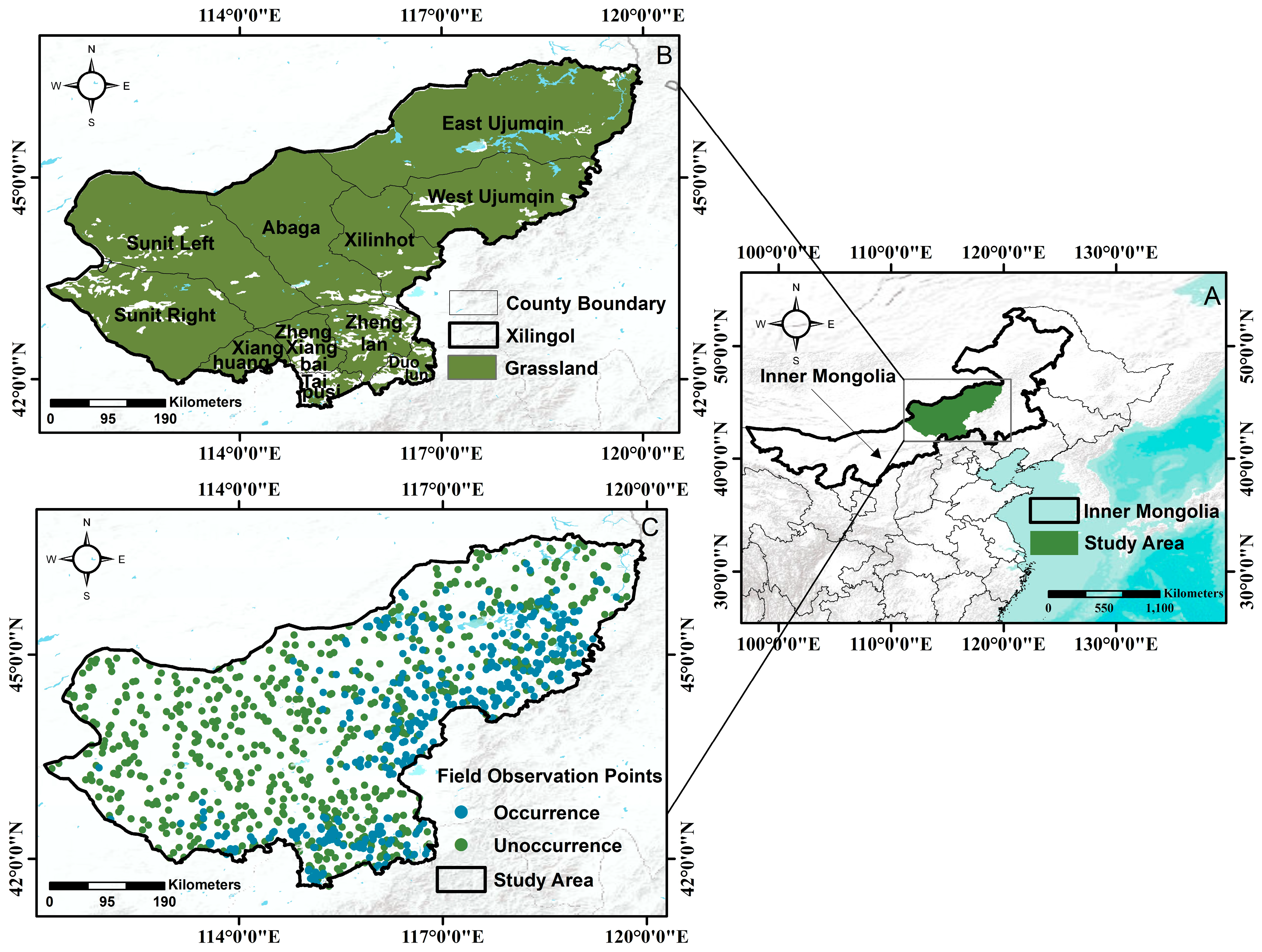
The Xilingol region, situated in the central part of the Inner Mongolia Autonomous Region, China, spans geographical coordinates between 41.57° and 46.77°N and 111.14° and 119.98°E (Figure 1). Encompassing a land area of 257,000 km², the region is home to approximately one million residents and is divided into 12 administrative counties [39]. Xilingol lies within the temperate arid and semi-arid climate zones, with grasslands covering an area of 192,512 km², accounting for 95.03% of the total area [40]. These grasslands are categorized into three distinct types—meadow, typical, and desert—distributed from east to west [41]. The region experiences an average annual temperature of 1–2 °C, with minimum temperatures dropping to −20 °C and maximum temperatures reaching 21 °C [42]. Relative humidity remains below 60% annually, while evaporation rates range from 1500 to 2700 mm, increasing from east to west [40]. Precipitation averages 200–300 mm per year, primarily concentrated during the vegetation growth season, and decreases gradually from east to west, reflecting significant regional variations [42]. The diverse grasslands and climatic conditions in Xilingol support a variety of grasshopper species, including Dasyhippus barbipes, Oedaleus decorus asiaticus, Anapodisma parabe, and Euchorthippus micropterus [43]. Therefore, this study considers grasshopper communities as a whole in Xilingol, with emphasis on the dominant species that collectively drive grassland degradation and ecological imbalance.

2.2. Data Acquisition and Processing

2.2.1. Satellite Data

Satellite data from 2017 to 2023, precisely aligned with the life cycle stages of grasshoppers, were collected and processed using the Google Earth Engine platform. The MOD09A1.061 product was used to derive the soil salinity index, which was examined for the egg, nymph, and adult phases. This dataset features a spatial resolution of 1 km and a temporal resolution of 8 days. The MOD11A1.061 product was also applied to gather minimum and mean land surface temperature (LST) data, focusing on the egg, nymph, and adult stages, with a spatial resolution of 1 km and a temporal resolution of 1 day. Furthermore, the MOD13A2.061 product provided the Normalized Difference Vegetation Index (NDVI), which was processed to estimate above-ground biomass (AB) for the nymph stage. The NDVI dataset has a spatial resolution of 1 km and a temporal resolution of 16 days.

2.2.2. Meteorological Data

Meteorological data from 2017 to 2023, corresponding to the developmental stages of grasshoppers, were collected and processed using the Google Earth Engine. Mean precipitation data, covering the egg, nymph, and adult stages, were sourced from the Global Precipitation Measurement (GPM) v6 dataset, with a spatial resolution of 11,132 m and a temporal resolution of monthly intervals. Additionally, mean specific humidity data for the egg and adult stages, as well as soil moisture data for all three developmental phases, were obtained from the Famine Early Warning Systems Network (FEWSNET) Land Data Assimilation System (FLDAS). The specific humidity dataset had a spatial resolution of 11,132 m and a temporal resolution of 1 day. In comparison, the soil moisture data had a spatial resolution of 11,132 m and a monthly temporal resolution.

2.2.3. Soil, Vegetation, and Topography Data

Soil characteristics, such as sand content, organic carbon, bulk density, nitrogen (5–15 cm depth), pH (5–15 cm depth), and clay content (5–15 cm depth), were acquired from the SoilGrids 250 m database (accessible at https://www.soilgrids.org (accessed on 6 March 2025)). Vegetation and soil type information were derived from the 1:1,000,000 national database, which was last updated in 2019. Topographic data was obtained from the Geospatial Data Cloud platform of the Chinese Academy of Sciences. These datasets—soil, vegetation, and topography—were considered static factors, as they typically do not change significantly within the study area. All satellite, meteorological, soil, and topographic data were collected and processed using the Google Earth Engine. Pre-processing steps, including mosaicking, masking, and reprojection, were performed, and all datasets were resampled to a consistent spatial resolution of 1 km.

2.2.4. Landscape Data

The landscape metrics used in this study were the patch area and the Contiguity Index; both derived from the vegetation-type dataset described in Section 2.2.3. The vegetation-type map was first converted into a categorical raster, where each contiguous group of cells with the same vegetation type was treated as an individual patch.

Patch-based landscape metrics were calculated using FRAGSTATS 4.3 (available at https://www.fragstats.org/index.php/downloads). Patch area (AREA, m²) describes the size of each vegetation patch and reflects the extent of continuous habitat. The Contiguity Index (CONTIG) quantifies the spatial connectedness of cells within a patch based on cell adjacency, with higher values indicating more compact and less fragmented patches. Both metrics were computed at the patch level using an 8-neighbor adjacency rule and then exported as raster layers with the exact spatial resolution as the vegetation-type dataset.

The resulting landscape-metric rasters were then overlaid with the analysis grid, and the values of patch area and Contiguity Index corresponding to each sampling unit were extracted and used as landscape-structure predictor variables in the grasshopper habitat suitability models.

2.2.5. Field Survey Data

Data for this research were collected through on-site assessments conducted between 2018 and 2023. The study complied with the agricultural norms set by the People’s Republic of China (NY/T 1578–2007, rules for investing locusts and grasshoppers in grassland). Each grassland area was regarded as a primary unit of study. Survey plots were established at intervals of at least 10 km, with each plot measuring 1 km by 1 km to align with the spatial scale of the environmental data. Within each plot, 10 sub-plots of 1 m by 1 m were randomly selected to document location details, grasshopper abundance, species identification, and population density. Observations were conducted during the nymph and adult phases from May to July, between 9:00 AM and 5:00 PM on clear days. In total, grasshopper presence was recorded at 649 locations and absence at 709 locations, as depicted in Figure 1C.

2.3. Analysis Process

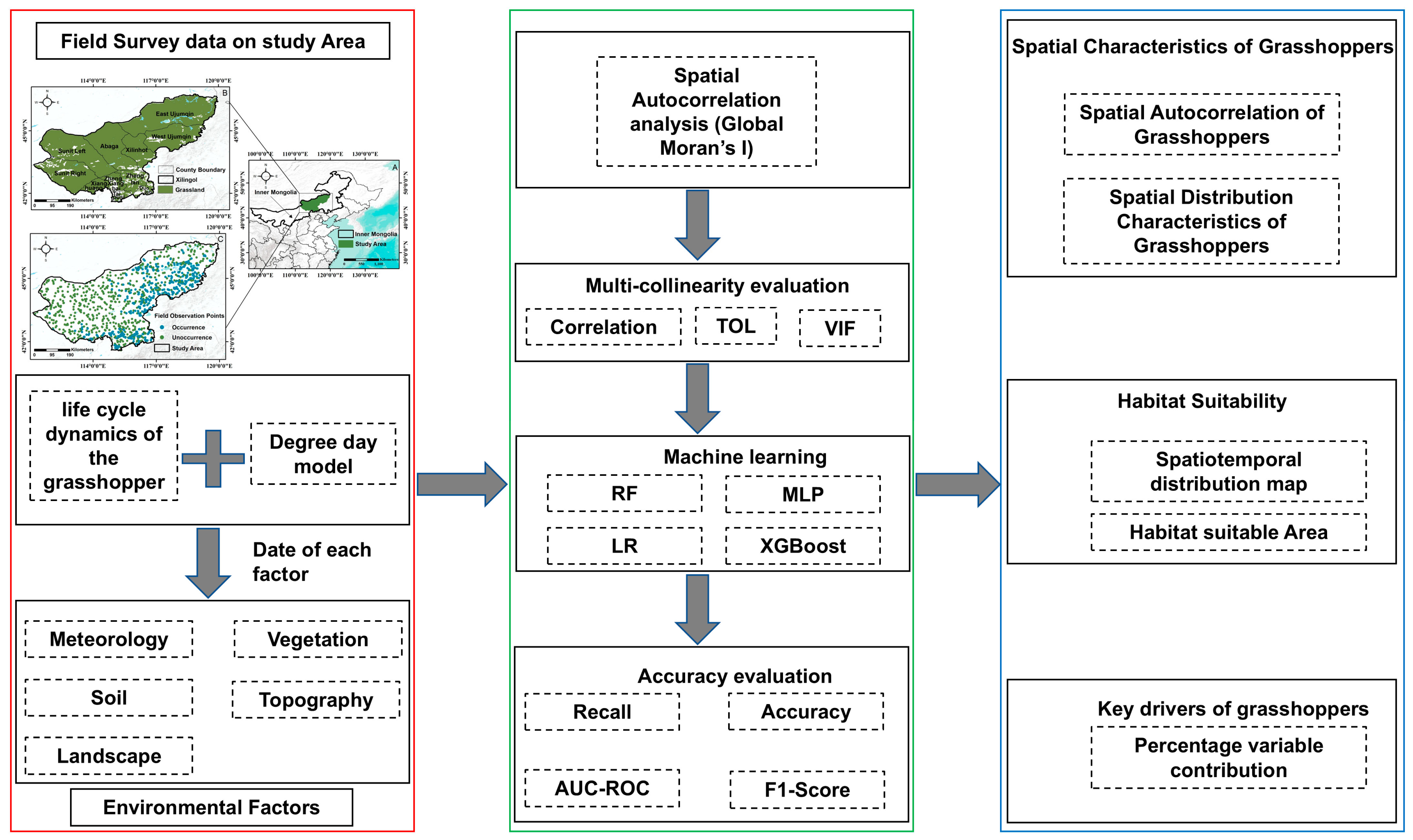
The methodological framework adopted in this study, illustrated in Figure 2, integrates field survey data, environmental variables, and machine learning models to evaluate grasshopper habitat suitability in the Xilingol region. Grasshopper developmental stages were aligned with ecological conditions using a degree-day (DD) framework, which provided the temporal basis for selecting habitat variables. A total of 29 factors representing meteorological, vegetation, topographic, soil, and landscape characteristics were assembled to describe habitat conditions. To minimize redundancy, multicollinearity among variables was tested using correlation analysis, tolerance (TOL), and variance inflation factor (VIF). Spatial patterns of grasshopper occurrence, based on field data collected between 2018 and 2023, were analyzed using the global Moran’s I index to evaluate distribution clustering. Habitat suitability was then modeled through four machine learning algorithms—Random Forest (RF), Logistic Regression (LR), Extreme Gradient Boosting (XGBoost), and Multi-Layer Perceptron (MLP)—with predictive performance measured by AUC-ROC, F1-score, recall, and overall accuracy. The most accurate model was used to produce suitability maps and delineate potential distribution areas. At the same time, variable importance analysis quantified the relative contribution of each environmental factor, thereby identifying the dominant drivers influencing grasshopper habitats in the Xilingol region.

2.3.1. Development of a Grasshopper Monitoring Indicator System

To construct a reliable monitoring framework for grasshopper habitats, we systematically identified environmental variables known to influence their distribution and population dynamics. Grasshopper occurrence is shaped by the interaction of meteorological conditions, vegetation structure, soil properties, topographic heterogeneity, and ecological context [4,44]. Temperature strongly determines development rates and life cycle progression [24], while vegetation regulates feeding behavior and oviposition [23]. Soil moisture governs egg survival [32], and altitude indirectly constrains distributions by altering microclimates [45]. These factors act synergistically, with their relative importance varying across regions, underscoring the need for a comprehensive, multi-factorial indicator system. We therefore compiled habitat variables in five categories—meteorology, vegetation, soil, topography, and ecology—and selected 29 representative indicators based on ecological relevance, measurability using remote sensing or environmental datasets, and spatial applicability across the diverse landscapes of the Xilingol League. These indicators were then integrated into a standardized monitoring framework to assess habitat suitability and forecast outbreak risk.

Since temperature-driven development is central to grasshopper population dynamics, we incorporated a degree-day (DD) model to quantify thermal requirements for growth [46]. The grasshopper life cycle consists of three stages—egg, nymph, and adult [47]—all of which are highly temperature-dependent [48]. Development requires both a lower threshold temperature and the accumulation of sufficient heat units; otherwise, growth halts, and diapause is induced [49]. In this study, the DD model utilized daily temperature data, as described in Section 2.2.1, as input. For each grid cell and day, we identified whether the daily mean temperature exceeded a lower developmental threshold obtained from previous experimental and field studies on grasshopper thermal biology [50,51]. When this threshold was exceeded, the surplus temperature above the threshold was considered effective heat accumulation for that day. These daily values were then summed over time to obtain cumulative thermal conditions for each location and year. Using stage-specific cumulative heat requirements reported in the literature [51,52], we then approximated the timing of key life stages, including egg hatching, nymphal development, and adult activity, across the Xilingol League. In this way, the DD model provided spatially explicit information on the thermal environment and estimated phenological windows for grasshopper development. Seasonally varying environmental indicators were subsequently averaged or accumulated within these DD-defined windows, ensuring that the predictor variables in the habitat suitability models reflected the conditions experienced by grasshoppers during their main development and activity periods rather than simple calendar-based averages [53].

Intercorrelations among environmental factors within the same category could compromise the accuracy of the model’s predictions [54]. To reduce redundancy among predictors, we tested for multicollinearity using the Variance Inflation Factor (VIF), Tolerance (TOL), and Spearman correlation coefficients (SCC). A TOL < 0.1, VIF > 5, or SCC ≥ 0.7 indicated potentially problematic relationships between variables [55], and such variables were excluded from the final indicator set.

2.3.2. Assessment of Global Spatial Autocorrelation in Grasshopper Occurrence

To examine spatial dependence in grasshopper occurrence, we employed Global Moran’s I statistic, a widely used measure of spatial autocorrelation that evaluates whether spatial patterns are clustered, dispersed, or random. Moran’s I ranges from −1 (perfect dispersion) to +1 (ideal clustering), with values near zero indicating random distributions.

The analysis was conducted annually from 2018 to 2023 using grasshopper occurrence data aggregated at the county level. Statistical significance of the Moran’s I values was assessed using associated z-scores and p-values, derived from randomization tests. Following conventional thresholds, a z-score greater than 1.96 (p < 0.05) was considered evidence of significant clustering, while a z-score less than −1.96 (p < 0.05) indicated significant dispersion [56].

To aid interpretation, the significance results were visualized using probability distributions of the test statistics. Spatial patterns were classified into three categories: dispersed, random, or clustered. This procedure ensured that the spatial structure of grasshopper occurrence could be rigorously evaluated across multiple years.

2.3.3. Machine Learning Models to Extract Habitat Suitability

• Random Forest (RF)

Random Forest is an advanced ensemble learning method that combines the outputs of numerous decision trees to improve the model’s reliability and precision [57]. In the training process, individual decision trees are built using a randomly selected portion of the training dataset, known as bootstrapping, and a random subset of features, a technique called feature bagging [58]. This strategy introduces diversity among the trees, reducing the risk of overfitting and enhancing the model’s ability to generalize to new data. Random Forest is highly effective for managing high-dimensional data and can accurately model complex interactions between variables, making it an ideal choice for challenging prediction problems.

In our study, the model was optimized via a 5-fold cross-validated grid search. Key hyperparameters tuned included the number of trees (n_estimators: 100, 300, 500), the maximum depth of trees (max_depth: 10, 20, None), and the minimum number of samples required to split a node (min_samples_split: 2, 5). We configured the final Random Forest model with 500 trees and employed balanced class weights to address potential class imbalance in the dataset [59,60]. The choice of 500 trees was guided by previous studies reporting stable performance gains beyond 300–500 trees [61], the grid search results, which indicated optimal performance at this value, and our preliminary analyses indicated that model accuracy plateaued after this point. This configuration allowed the model to remain sensitive to minority classes while maintaining strong predictive performance. The hyperparameter tuning process used log loss as the performance metric to be minimized. The final prediction of the Random Forest is obtained by aggregating the outputs of all decision trees, where each tree contributes equally to the ensemble result. This aggregation can be expressed as:

$$\widehat{y}={\displaystyle \frac{1}{T}}{\displaystyle \sum _{t=1}^T{h}_t}(x)$$

(1)

where $\widehat{y}$ is the predicted probability, $T$ is the number of trees, and $h_t$$(x)$ is the prediction of the t-th tree.

2.

Multilayer Perceptron (MLP)

A Multi-Layer Perceptron (MLP) is a feedforward neural network composed of multiple fully connected layers of nodes, enabling the modeling of complex nonlinear relationships between inputs and outputs [62,63]. This architecture makes MLPs powerful tools for classification and regression tasks when sufficient data are available. The activation of each neuron can be expressed as:

$$h_i^l=g\left({\displaystyle \sum _{k=1}^m{w}_k^l}{h}_k^{l-1}\right)$$

(2)

In this equation, $g$ represents the activation function, $w_k^l$ is the weight of the $k$-th neuron in layer $l$, $h_k^{l-1}$ is the activation of the $k$-th neuron in the preceding layer $l-1$, $l$ indicates the layer index, $i$ is the neuron index, and $m$ is the count of neurons in the layer $l$ [64]. In this study, we conducted a 5-fold cross-validated grid search to tune the network architecture and learning parameters. The search space included the number of hidden layers (1, 2, 3), the number of neurons per layer (64, 128, 256), the learning rate for the Adam optimizer (learning_rate_init: 0.001, 0.01), and the L2 regularization penalty (alpha: 0.0001, 0.001). The best-performing configuration consisted of three hidden layers with 256, 128, and 64 neurons, which effectively balanced predictive accuracy and the risk of overfitting. The use of progressively fewer neurons across layers followed common design principles of hierarchical feature extraction [65]. We applied the Rectified Linear Unit (ReLU) activation function to introduce nonlinearity and accelerate convergence [66], while optimization was performed using the Adam algorithm [67,68]. To further improve generalization, early stopping was employed with a validation set and a patience of 10 epochs.

3.

Extreme Gradient Boosting (XGBoost)

Extreme Gradient Boosting (XGBoost) is an advanced and efficient implementation of gradient boosting that builds decision trees sequentially, with each tree correcting the residual errors of the previous ones [69]. This iterative design, combined with regularization, makes XGBoost highly effective for modeling complex, nonlinear relationships in large and high-dimensional datasets [70]. A further advantage of XGBoost is its ability to handle missing values and noisy inputs, which is particularly relevant for ecological data derived from multiple sources.

The general loss function in XGBoost is expressed as:

$$L(\varphi )={\displaystyle \sum _{i}l}({\widehat{y}}_i,y_i)+{\displaystyle \sum _k\Omega }(f_k)$$

(3)

In this equation, the first component represents the loss function, with $y_i$ and ${\widehat{y}}_i$ denoting the actual and forecasted values, respectively. To mitigate overfitting and address complexity issues, the following equation is applied:

$$\Omega (f)=\gamma T+\frac{1}{2}\lambda \Vert w{\Vert }^2$$

(4)

Here, $T$ corresponds to the number of leaves in the tree, and $w$ signifies the score attributed to each leaf.

In this study, the XGBoost model was configured following a 5-fold cross-validated grid search. We tuned several key parameters, including the number of boosting rounds (n_estimators: 100, 300, 500), the maximum tree depth (max_depth: 3, 6, 9), the learning rate (learning_rate: 0.01, 0.1), and the subsample ratio of columns (colsample_bytree: 0.8, 1.0). The final model used 500 boosting rounds (n_estimators = 500) and a fixed random seed (random_state = 123) to ensure reproducibility. To address class imbalance, the parameter scale_pos_weight was set to 2, which increased the weight of minority (presence) cases and improved predictive sensitivity. This configuration provided stable performance while effectively capturing the relationships between grasshopper occurrence and environmental predictors.

4.

Logistic Regression (LR)

Logistic Regression (LR) is a widely used statistical method for binary classification that models the probability of occurrence using a logistic function. It is valued for its interpretability and computational simplicity, and it often serves as a benchmark against which more complex machine learning models are compared. The probability of occurrence is estimated as [71]:

$$P={\displaystyle \frac{1}{1+e^{-({\beta }_0+{\beta }_1{x}_1+{\beta }_2{x}_2+\dots +{\beta }_n{x}_n)}}}$$

(5)

Here, P is the probability of grasshopper presence. β₀ is the model’s intercept, β₁, β₂,…, β_n are the coefficients and x₁, x₂,…, x_n are the input features. In this study, we applied LR with balanced class weights to account for class imbalance in the dataset. To optimize the model, we performed a 5-fold cross-validated grid search over the inverse regularization strength parameter C (values: 0.1, 1, 10) and the penalty norm (L₁, L₂). The L₂ penalty with C = 1 was selected based on this process. This adjustment increased the influence of minority (presence) cases, improving sensitivity and yielding more reliable predictions of grasshopper distribution.

Grasshopper monitoring outcomes were categorized into three suitability classes according to their occurrence probabilities: low suitability (0 < P ≤ 0.5), moderate suitability (0.5 < P ≤ 0.7), and high suitability (0.7 < P ≤ 1) [72]. To identify the key environmental factors shaping habitat suitability, we employed Shapley Additive Explanations (SHAP), which quantifies the contribution of each predictor to model outputs and provides a consistent, interpretable measure of feature importance across the study area [73].

3. Results

3.1. Grasshopper Monitoring Indicator System

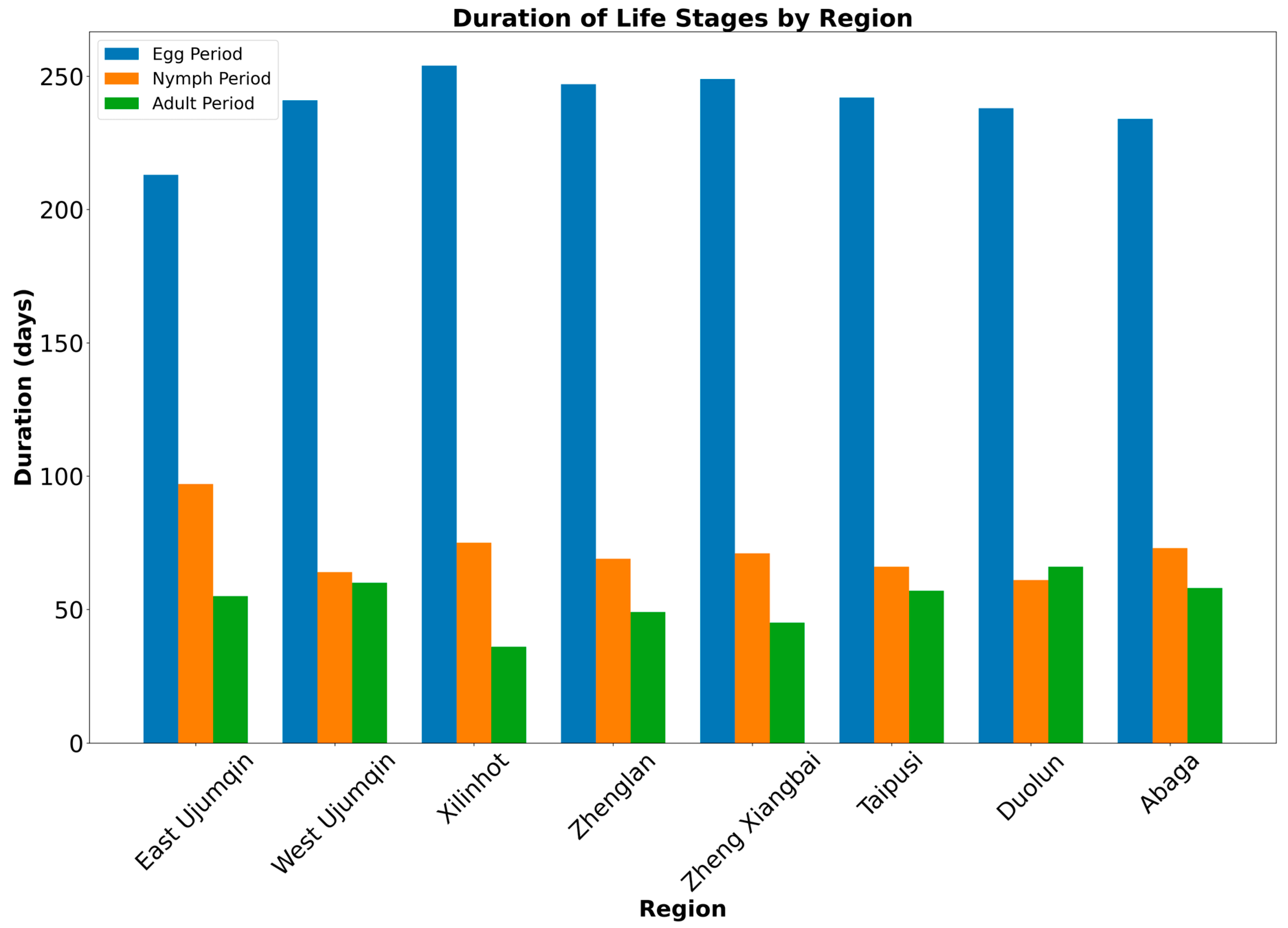
Drawing on the developmental mechanisms of grasshoppers, we applied a degree-day (DD) model to estimate the duration of developmental periods for grasshoppers across each county. The duration of grasshopper life stages varied substantially across regions (Figure 3). The egg period was consistently the longest stage, ranging from 213 days in East Ujumqin to 254 days in Xilinhot, with most regions exhibiting egg periods exceeding 235 days. This pattern underscores the importance of overwintering in the grasshopper life cycle. The nymph period displayed greater regional variation, lasting 97 days in East Ujumqin but only 61 days in Duolun. Thermal accumulation patterns can explain these differences: in East Ujumqin, the initial developmental temperature was reached in mid-April, but nighttime conditions often fell below the threshold, restricting degree-day accumulation to daytime and prolonging development. In contrast, Duolun entered the incubation period with average temperatures of 10–12 °C, which enabled faster accumulation of effective heat units and thus shortened the nymphal stage. The adult period was generally shorter than the nymph stage but still varied across regions. The longest adult phases occurred in Duolun (66 days) and West Ujumqin (60 days), while the shortest was observed in Xilinhot (36 days). In Duolun, the extended adult stage likely reflects favorable summer thermal conditions that prolonged reproductive activity. In contrast, in Xilinhot, higher early-summer temperatures may have accelerated maturation, leading to a shorter lifespan. Overall, these results indicate that the egg stage predominates in the grasshopper life cycle across all regions, while the nymph and adult stages are more sensitive to local thermal regimes. Extended nymphal development in East Ujumqin and prolonged adult longevity in Duolun underscore the significant impact of regional climate and heat accumulation on grasshopper phenology.

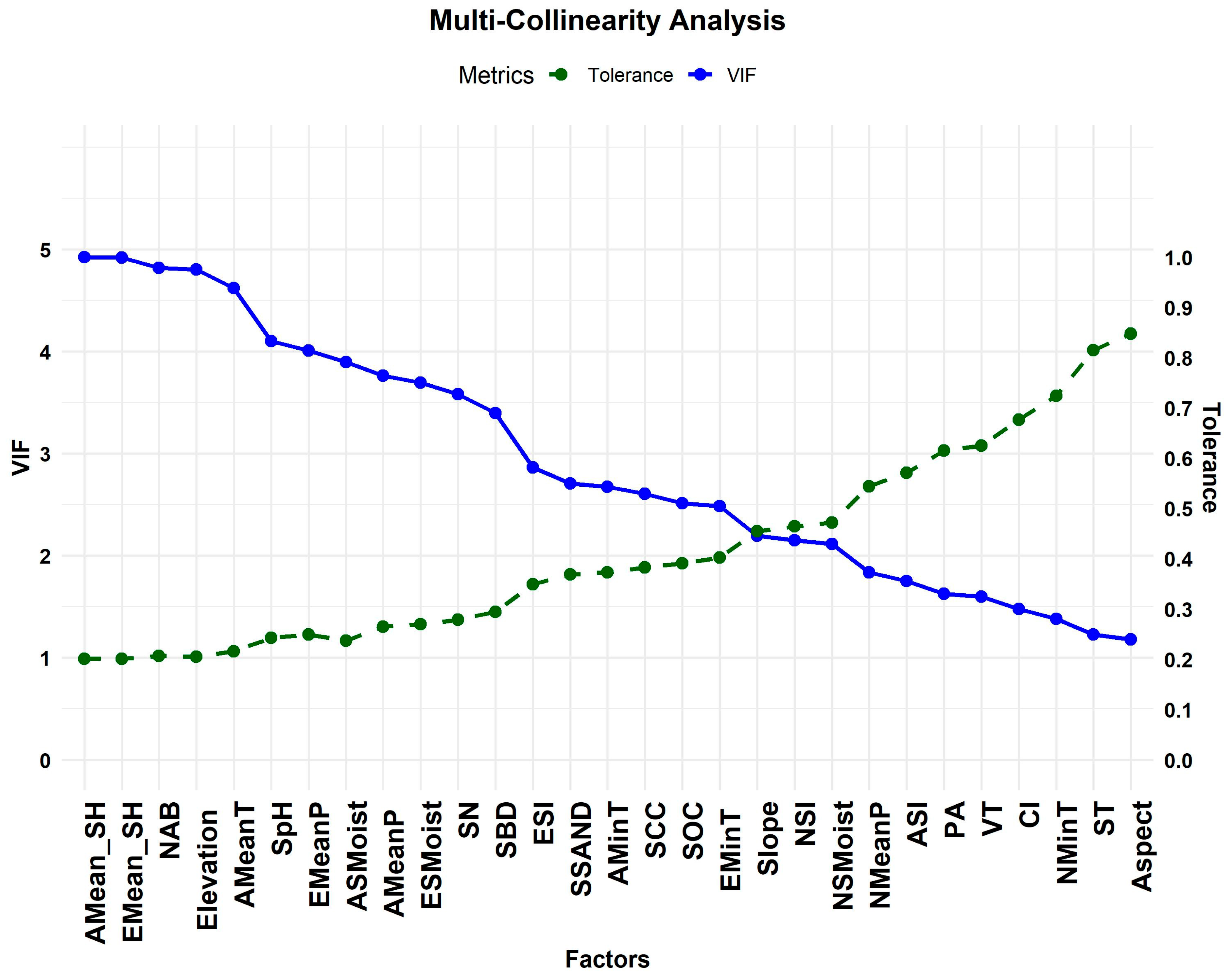
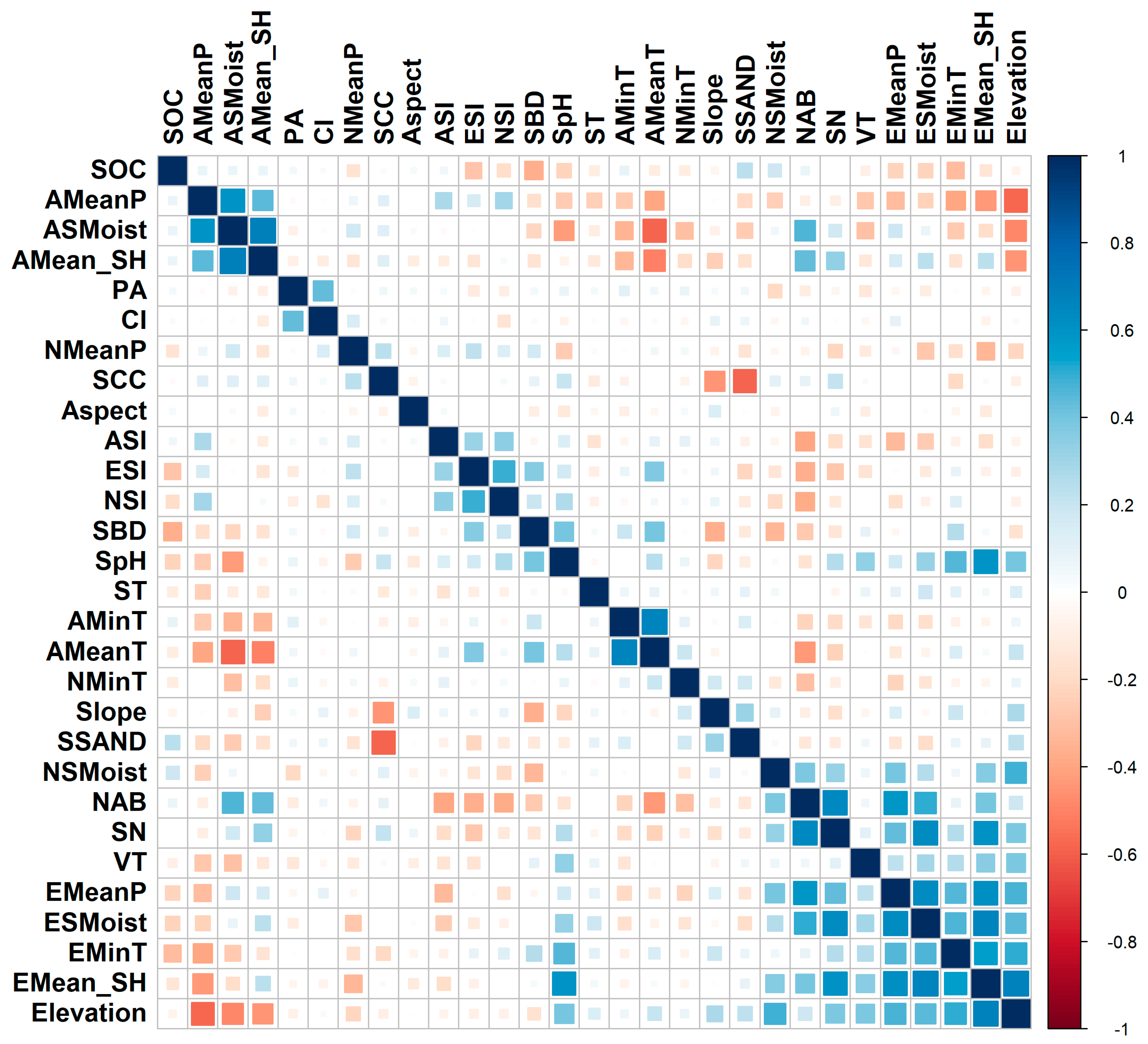
Building on these developmental results, we identified habitat factors associated with each stage and tested them for multicollinearity (Figure 4 and Figure 5) to ensure the robustness of our indicator selection. TOL values ranged from 0.201 to 0.848, with the lowest observed for AMean_SH and the highest for Aspect (Figure 4). Similarly, VIF values ranged from 1.178 for Aspect to 4.922 for AMean_SH (Figure 4). Since all TOL values remained above 0.1 and all VIF values below 5, none of the predictors exhibited problematic collinearity. Spearman’s correlation coefficients provided additional confirmation, with all values falling below the exclusion threshold of |r| ≥ 0.70 (Figure 5). The strongest positive correlation was found between AMean_SH and ASMoist (r = 0.69), while the strongest negative correlation occurred between AMeanT and ASMoist (r = −0.59). These results confirm that the selected predictors were sufficiently independent and could be retained for subsequent modeling. The final set of factors chosen for our study, as detailed in

Table 1. Environmental factors. Altogether, there are 29 factors.

Category	Factors	Factors in Grasshopper Development Period	Abbreviation	Data Source	Spatial Resolution	Temporal Resolution
Soil	Soil Moisture	Egg period	ESMoist	FLDAS	11,132 m	Monthly
		Nymph period	NSMoist	FLDAS	11,132 m	Monthly
		Adult period	ASMoist	FLDAS	11,132 m	Monthly
	Soil Salinity index	Egg period	ESI	MOD09A1.061	1 km	8 days
		Nymph period	NSI	MOD09A1.061	1 km	8 days
		Adult period	ASI	MOD09A1.061	1 km	8 days
	Soil Sand	static factor	SSAND	Soil Grids	250 m
	Soil Organic Carbon	static factor	SOC	Soil Grids	250 m
	Soil Ph	static factor	SpH	Soil Grids	250 m
	Soil Bulk Density	static factor	SBD	Soil Grids	250 m
	Soil Nitrogen	static factor	SN	Soil Grids	250 m
	Soil Clay Content	static factor	SCC	Soil Grids	250 m
	Soil Type	static factor	ST	Chinese Academy of Sciences	250 m
Topography	Elevation	static factor	Elevation	Chinese Academy of Sciences	90 m
	Slope	static factor	Slope	Chinese Academy of Sciences	90 m
	Aspect	static factor	Aspect	Chinese Academy of Sciences	90 m
Landscape	Patch Area	static factor	PA	Chinese Academy of Sciences	1 km
	Contiguity Index	static factor	CI	Chinese Academy of Sciences	1 km
Meteorology	Minimum land surface temperature	Egg period	EMinT	MOD11A1.061	1 km	1 day
		Nymph period	NMinT	MOD11A1.061	1 km	1 day
		Adult period	AminT	MOD11A1.061	1 km	1 day
	Mean land surface temperature	Adult period	AMeanT	MOD11A1.061	1 km	1 day
	Mean specific humidity	Egg period	EMean_SH	FLDAS	11,132 m	1 day
		Adult period	AMean_SH	FLDAS	11,132 m	1 day
	Mean Precipitation	Egg period	EMeanP	GPM	11,132 m	Monthly
		Nymph period	NMeanP	GPM	11,132 m	Monthly
		Adult period	AMeanP	GPM	11,132 m	Monthly
Vegetation	Aboveground biomass	Nymph period	NAB	MOD13A2	1 km	16 days
	Vegetation type	Static factor	VT	Chinese Academy of Sciences	1 km

, includes: AMinT, AMeanT, NMinT, AMeanP, ASMoist, AMean_SH, SOC, PA, CI, NMeanP, SCC, NSMoist, NAB, SN, VT, EMeanPre, ESMoist, EMinLST, EMeanSH, Elevation, ST, Slope, SSAND, Aspect, SpH, ASI, ESI, NSI, and SBD.

3.2. Global Spatial Autocorrelation of Grasshopper Occurrence (2018–2023)

Global spatial autocorrelation, assessed annually using Moran’s I, consistently revealed a clustered distribution of grasshopper densities between 2018 and 2023 (Figure S1). In 2018, Moran’s I was 0.93 (z = 15.62, p < 0.001), followed in 2019 by a slightly lower but still pronounced value of 0.54 (z = 15.29, p < 0.001). Clustering then intensified in 2020 and 2021, when Moran’s I reached 0.95 in both years, accompanied by the highest z-scores of the series (z = 19.22, p < 0.001). In 2022, the degree of spatial autocorrelation declined modestly (Moran’s I = 0.74, z = 2.74, p < 0.001), yet the pattern remained highly significant. A marginal rebound was observed in 2023, when Moran’s I rose to 1.00 (z = 2.04, p = 0.040), confirming persistence of clustering at the 5% significance level.

Collectively, these findings demonstrate six consecutive years of statistically significant positive spatial autocorrelation, highlighting the enduring and non-random spatial structure of grasshopper populations across the study area.

3.3. Habitat Suitability of Grasshopper by Machine Learning

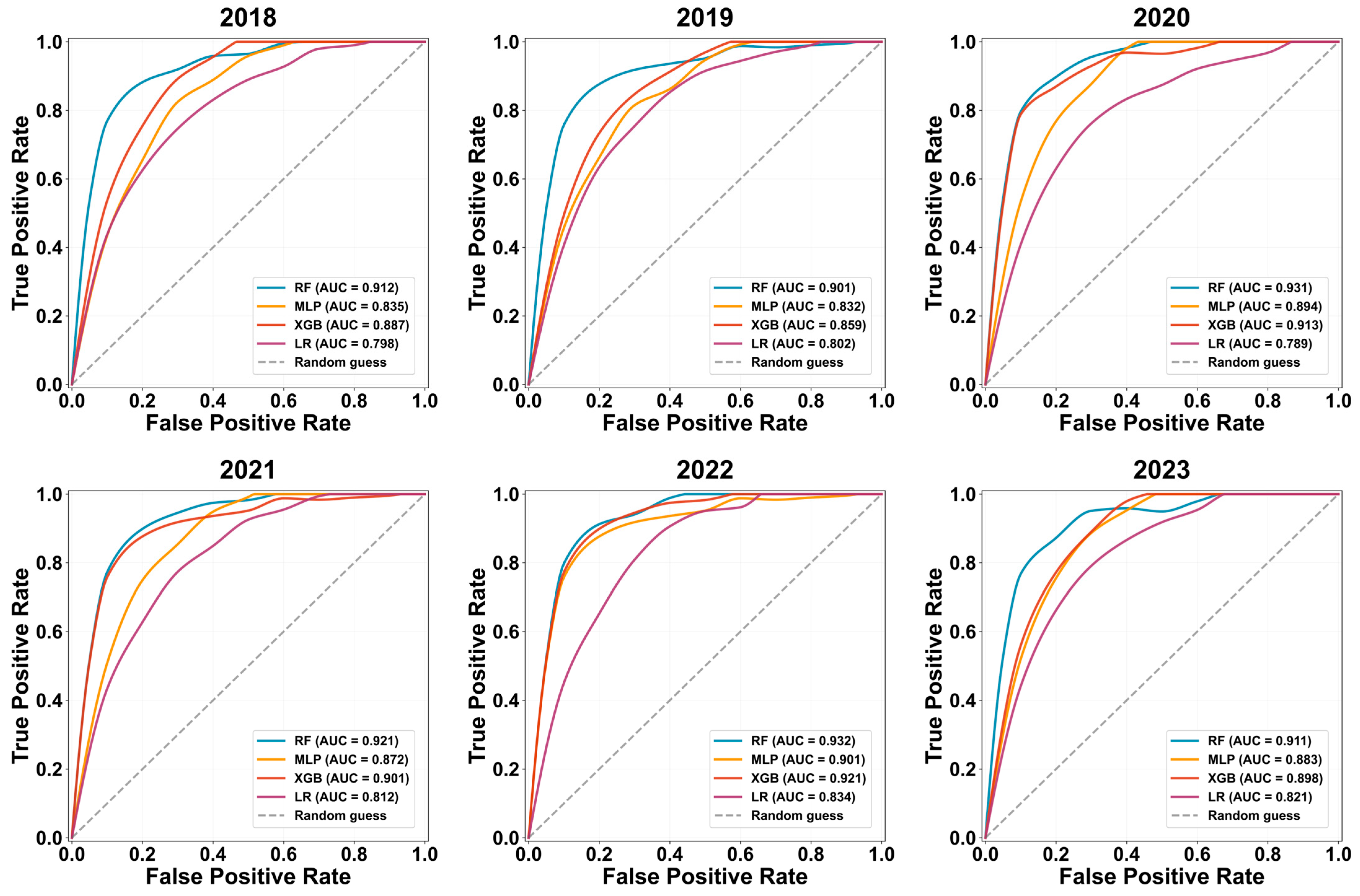
The evaluation results for the four machine learning models (Figure 6;

Table 2. Evaluation Results of the Four Machine Learning Models.

Year	Model	RMSE	AUC	F1-Score	Recall	Accuracy
2018	RF	0.110	0.912	0.860	0.894	0.881
	MLP	0.150	0.835	0.780	0.810	0.800
	XGB	0.125	0.887	0.830	0.850	0.840
	LR	0.160	0.798	0.740	0.770	0.760
2019	RF	0.105	0.901	0.855	0.885	0.875
	MLP	0.155	0.832	0.770	0.800	0.790
	XGB	0.135	0.859	0.805	0.830	0.820
	LR	0.155	0.802	0.740	0.765	0.765
2020	RF	0.100	0.931	0.880	0.910	0.895
	MLP	0.130	0.894	0.830	0.850	0.835
	XGB	0.110	0.913	0.860	0.880	0.870
	LR	0.170	0.789	0.710	0.735	0.742
2021	RF	0.090	0.921	0.870	0.900	0.885
	MLP	0.120	0.872	0.810	0.830	0.825
	XGB	0.115	0.901	0.835	0.855	0.845
	LR	0.140	0.812	0.755	0.780	0.771
2022	RF	0.095	0.932	0.880	0.905	0.890
	MLP	0.130	0.901	0.835	0.855	0.845
	XGB	0.100	0.921	0.860	0.880	0.870
	LR	0.135	0.834	0.765	0.790	0.781
2023	RF	0.110	0.911	0.850	0.875	0.865
	MLP	0.120	0.883	0.820	0.840	0.835
	XGB	0.105	0.898	0.835	0.855	0.838
	LR	0.138	0.821	0.745	0.770	0.753

) indicated that the RF model consistently achieved higher predictive performance than the other three models. Across all years, the AUC of RF was greater than that of MLP, XGB, and LR, and its RMSE remained the lowest. Similarly, recall and F1-scores of RF were higher than those of the other models, confirming its superior ability to capture grasshopper occurrence patterns. XGB ranked second, with values close to those of RF, particularly in 2020 and 2022. MLP achieved moderate performance, while LR consistently produced the lowest accuracy and the highest RMSE. These results imply that RF, by effectively handling nonlinear relationships and complex feature interactions, outperformed XGB, MLP, and LR, and therefore proved to be the most reliable model for predicting grasshopper occurrence across years.

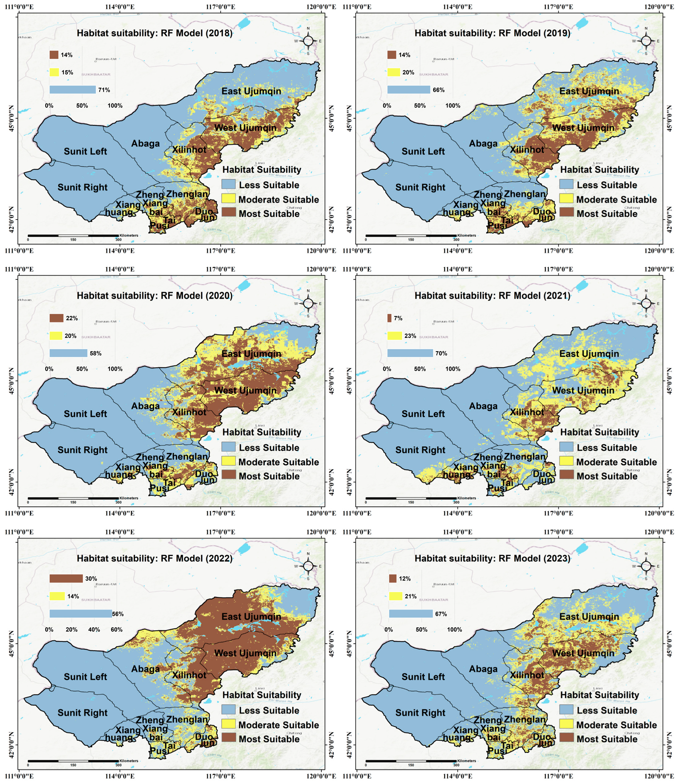
The RF model revealed pronounced spatial and temporal variation in grasshopper habitat suitability across the Xilingol League from 2018 to 2023, which was classified into three suitability levels (Figure 7). Across the study period, less suitable habitats consistently dominated, covering more than half of the region each year, while moderately suitable and most suitable habitats fluctuated substantially. Highly suitable habitats were primarily concentrated in East Ujumqin, West Ujumqin, and Xilinhot, with secondary centers in Duolun, Taipusi, Zhenglan, and Xianghuang. In contrast, Sunit Left, Sunit Right, and Abaga were persistently dominated by less suitable habitats.

In 2018, 71% of the area was classified as less suitable, with 15% classified as moderately suitable and 14% as most suitable, concentrated mainly in East and West Ujumqin and Xilinhot. In 2019, moderately suitable habitats expanded to 20%, while most suitable habitats remained at 14%, with increases in East and West Ujumqin. Suitability improved further in 2020, when most suitable habitats expanded to 22% and moderately suitable areas accounted for 20%, particularly in the northern and eastern parts of West Ujumqin, central Xilinhot, and northern Duolun. By 2021, however, the extent of most suitable habitats declined sharply to 7%, as East and West Ujumqin lost much of their suitable area, although Zhenglan, Xiang Huang, and Taipusi exhibited local increases. The peak occurred in 2022, when most suitable habitats reached 30% of the study area, the highest across all years. West Ujumqin held the largest share of highly suitable habitats (>20%), followed by notable expansions in East Ujumqin and southern Duolun. This sharp increase in 2022 can be attributed to a combination of favorable climatic and environmental factors. First, egg-stage minimum temperatures (EMinT) in East and West Ujumqin ranged from −31 °C to −29 °C, within the optimal range for grasshopper egg survival, thereby reducing egg mortality and enhancing hatching success; winter temperatures between −35 °C and −28 °C are generally favorable for grasshopper survival, whereas more extreme cold can cause high egg mortality [74]. Second, mean precipitation during the nymph stage (NMeanP) in 2022 was favorable, as increased rainfall supported vegetation growth, providing ample food for the grasshopper nymphs. In particular, the NMeanP during the nymph stage contributed to the development of high-quality vegetation, which was essential for nymph survival. Third, above-ground biomass (NAB) during the nymph stage was higher in 2022, with values peaking at 140 kg/hm³, providing abundant food for grasshopper nymphs, supporting their growth, and contributing to the expansion of suitable habitats. In 2023, however, the extent of most suitable habitats contracted again to 12%, with marked declines in West Ujumqin, Xilinhot, Duolun, and Taipusi, although East Ujumqin retained a relatively large share of moderately suitable habitats.

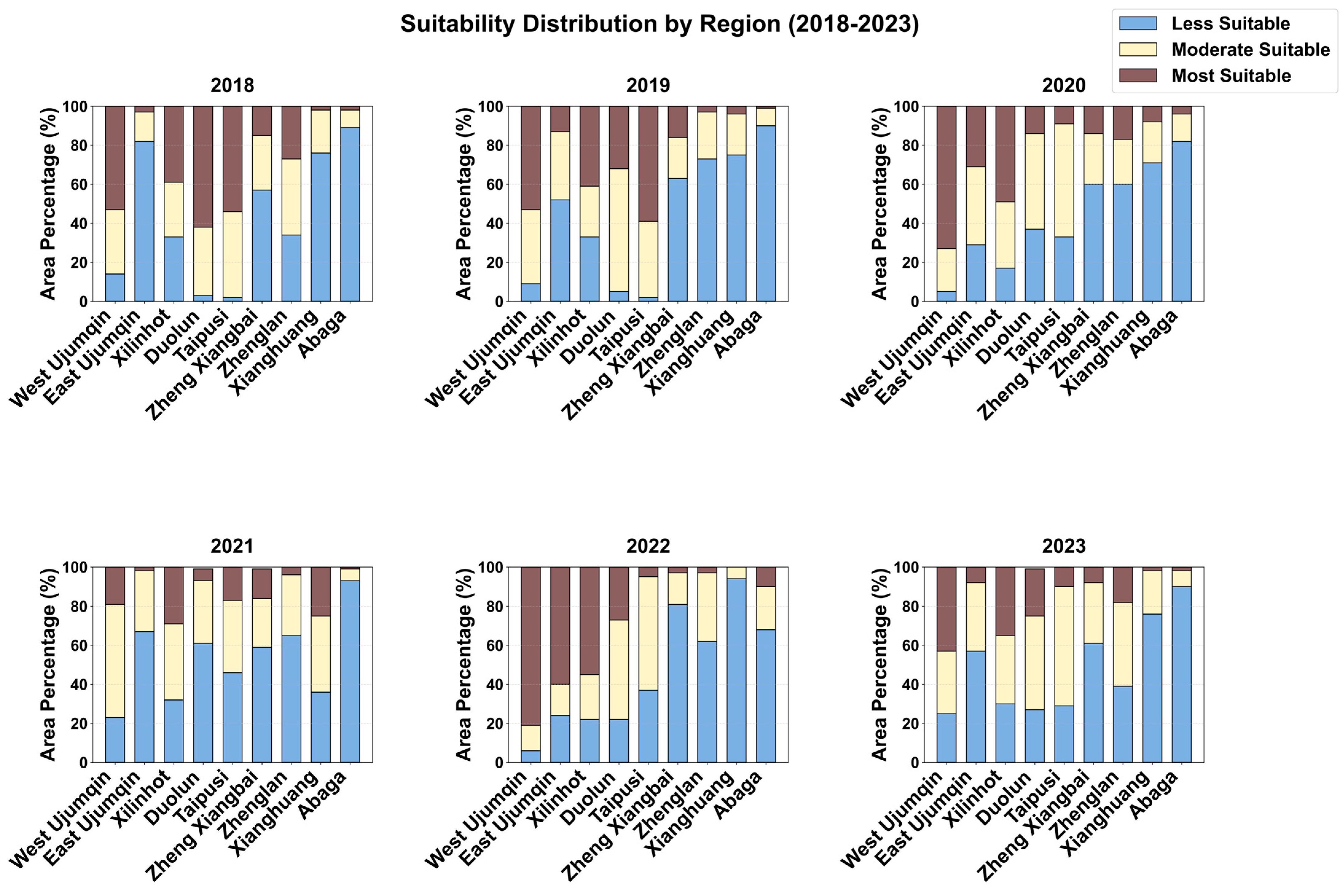
Regional distributions (Figure 8) provided further detail on these dynamics. East Ujumqin, West Ujumqin, and Xilinhot consistently contained the highest proportions of moderately and highly suitable habitats, reinforcing their roles as persistent centers of grasshopper suitability. In contrast, Abaga, Sunit Left, and Sunit Right were overwhelmingly less suitable throughout the study period, with grasshopper suitability remaining consistently low. Temporal fluctuations were most pronounced in East and West Ujumqin, which experienced repeated expansions and contractions of highly suitable areas, particularly the sharp increase in 2022, followed by the decline in 2023.

Overall, the results demonstrate that less suitable areas dominate grasshopper habitats across the Xilingol League; however, East Ujumqin, West Ujumqin, and Xilinhot consistently contain higher proportions of suitable habitats, providing favorable conditions for grasshopper occurrence. Substantial interannual variability, particularly the surge in suitability in 2022 and the contraction in 2023, underscores the sensitivity of grasshopper habitats to changing environmental conditions.

3.4. Habitat Factors Shaping Grasshopper Distribution Patterns

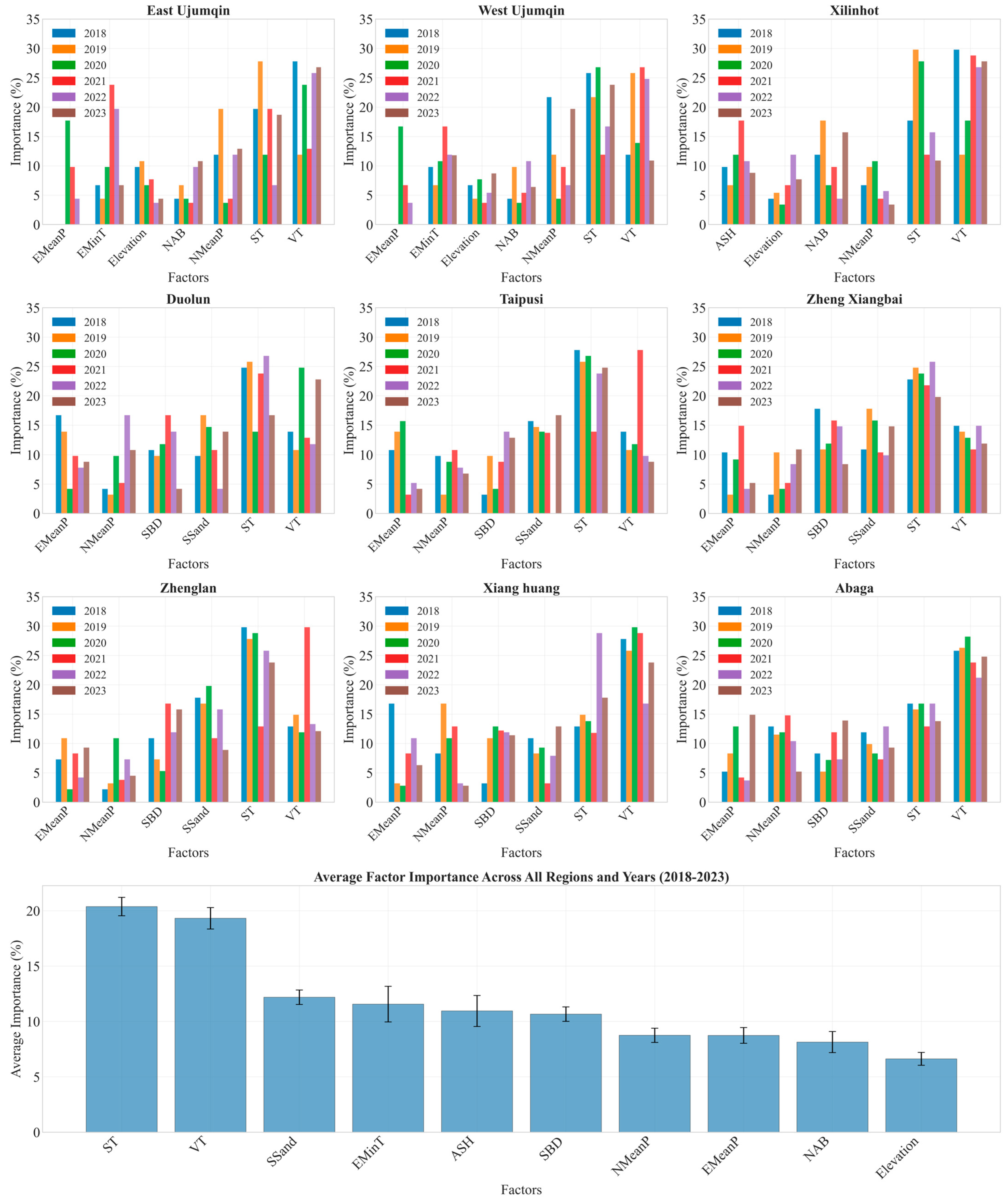
The feature importance analysis demonstrated that grasshopper habitat suitability across the Xilingol League was primarily governed by soil and vegetation factors, with consistent yet regionally variable contributions from climate and soil texture. On average, soil type (ST) and vegetation type (VT) were the most influential predictors, contributing 21.1% and 19.8%, respectively (Figure 9). Secondary influences included soil sand content (SSand, 12.6%) and egg-stage minimum temperature (EMinT, 11.3%), while adult-stage specific humidity (ASH, 10.9%) and soil bulk density (SBD, 10.8%) were moderately important. Precipitation-related variables (EMeanP, 8.7%; NMeanP, 8.8%) and nymph-stage aboveground biomass (NAB, 8.1%) contributed less consistently, and elevation was the least influential factor (<6%).

The dominance of soil and vegetation types can be explained by their direct links to key grasshopper life stages. Vegetation type (VT) mainly influences food quality and microhabitat conditions. Monocotyledonous grasses are often preferred host plants for many acridid species, providing optimal nutrition for nymph development and adult reproductive success [75], while dense or woody vegetation can hinder movement and oviposition. Similarly, soil type (ST) and its physical properties, such as texture and compaction, are essential for successful oviposition and egg overwintering, as female grasshoppers tend to lay their egg pods in well-drained soils with suitable textures [76]. Soil texture, indicated by sand content (SSand), directly impacts egg survival. Sandy or loamy soils promote drainage, preventing egg pods from becoming waterlogged, while allowing deeper penetration for egg-laying and offering better insulation against extreme winter cold. Conversely, clay-rich soils are more prone to compaction and water retention, which can cause anoxia and fungal growth, increasing egg mortality [32]. Soil bulk density (SBD) is an essential measure of soil compaction: low to moderate SBD indicates softer soils that are easier for females to excavate for oviposition, whereas highly compacted soils (high SBD) can physically block egg-laying and reduce habitat suitability [76].

Regional analyses revealed both consistent and contrasting drivers of suitability. In East Ujumqin, suitability was most strongly shaped by VT and ST in every year (up to 27.8% and 19.7%, respectively), while precipitation variables occasionally ranked highly, such as NMeanP (12.9%) in 2023. The Egg-stage Minimum Temperature (EMinT) also showed pronounced effects, peaking at 23.8% in 2021, reflecting the sensitivity of embryonic development to thermal thresholds. In West Ujumqin, ST and VT alternated as leading factors (each contributing >25%), while NMeanP consistently exerted strong influence (21.7% in 2018–2019 and 19.7% in 2023), highlighting the importance of rainfall during the nymph stage in this semi-arid area.

In Xilinhot, vegetation type consistently dominated (up to 29.8%), followed by ST, but other factors such as NAB (17.7% in 2019) and ASH (11.9–17.7% across years) repeatedly contributed, indicating that food supply and adult microclimatic humidity strongly modulated suitability in this central region. By contrast, Duolun was characterized not only by ST and VT but also by persistent contributions from soil-related factors: SBD (16.7%) and SSand (14.7–16.7%), alongside intermittent importance of precipitation (EMeanP up to 16.7%). These results suggest that both soil structure and rainfall strongly constrain suitability in this county. Taipusi followed a similar pattern, dominated by ST (27.8%) but with notable contributions from SSand and SBD (13–17%), while EMeanP was also influential in certain years (15.7%).

In the western counties, soil-related variables were even more decisive. In Zheng Xiangbai, ST was consistently the top predictor (19.8–25.8%), followed by SBD (14.8–17.8%) and VT (11.9–14.9%), with moderate contributions from SSand and precipitation. Similarly, Zhenglan displayed a distinctive dominance of ST (up to 29.8%) and SSand (up to 19.8%), often ahead of VT, underscoring the importance of soil texture and compaction. SBD ranked third in several years (10.9–16.8%), reinforcing the role of soil physical properties in determining oviposition suitability. In Xianghuang, VT was the leading predictor every year (23.8–29.8%), consistently followed by ST, while SBD and precipitation (NMeanP and EMeanP) played secondary roles. Finally, in Abaga, suitability was primarily shaped by VT and ST (VT 21.2–28.2%, ST 13.8–16.8%), with more minor but steady effects of SSand, SBD, and precipitation. Notably, EMeanP rose sharply in 2023 (14.9%), reflecting the importance of rainfall events in this otherwise less suitable region.

Taken together, these findings confirm that soil type and vegetation type are the dominant and universal drivers of habitat suitability, but the relative influence of other predictors varies geographically. East and West Ujumqin were additionally shaped by precipitation and egg-stage temperature; Xilinhot by vegetation, nymph-stage biomass, and adult-stage humidity; Duolun and Taipusi by soil bulk density, sand content, and rainfall; Zheng Xiangbai and Zhenglan by soil-related properties; and Abaga by vegetation with episodic rainfall effects. This regional heterogeneity reflects the different ecological constraints operating across the League. It demonstrates that the Random Forest model successfully captured both consistent drivers and local nuances of grasshopper habitat suitability.

4. Discussion

Grasshopper occurrence in temperate grasslands is shaped by a suite of interacting environmental drivers, including meteorological conditions, vegetation structure, soil characteristics, topography, and ecological context. For prediction and early-warning systems to be reliable, monitoring indicators must be carefully chosen to reflect these drivers in a way that captures both their biological relevance and regional variability. In this study, we linked a degree-day (DD) model with field survey data and the life cycle dynamics of grasshoppers to quantify developmental timing across the Xilingol League. By using thermal requirements to delimit egg, nymph, and adult stages, this approach provided a more biologically grounded framework than earlier methods that relied on empirical or fixed life cycle divisions [26,77]. As a result, the temporal alignment of environmental indicators with life-history processes improved, better capturing how climate and habitat factors regulate grasshopper occurrence.

To build a robust indicator system, 29 variables representing meteorology, vegetation, soil, topography, and landscape attributes were assembled and screened for redundancy using multicollinearity tests. This systematic selection ensured that the final indicators were both ecologically meaningful and statistically independent. Compared with previous studies that often selected predictors based on empirical knowledge or single-variable correlations [78,79], our framework incorporated multiple evaluation steps, including tolerance (TOL), variance inflation factor (VIF), and correlation thresholds. This dual focus on ecological significance and statistical rigor enhanced the reliability of the selected predictors for modeling habitat conditions.

Among the algorithms tested, Random Forest (RF) consistently outperformed MLP, XGBoost, and logistic regression (LR) in AUC, recall, and F1-scores. Its strength lies in capturing nonlinear relationships, integrating high-dimensional data, and maintaining robustness against noise and class imbalance. This performance underscores RF as the most effective approach for this ecological prediction task. The lower performance of the LR model compared to RF/MLP/XGBoost can be attributed to the linear assumptions of LR, which struggle to capture the complex, nonlinear interactions present in ecological data. Ensemble methods and neural networks, such as RF and XGBoost, perform better due to their ability to model these nonlinear relationships, providing more accurate predictions.

Building on these robust modeling results, we examined the spatiotemporal distribution of habitat suitability. Intense and persistent spatial clustering of grasshopper occurrence was evident from 2018 to 2023, as confirmed by Moran’s I. The RF-derived suitability maps revealed key ecological insights: less suitable habitats consistently dominated the League, but East Ujumqin, West Ujumqin, and Xilinhot repeatedly emerged as persistent centers of grasshopper activity. These regions combine favorable vegetation and soil with supportive climates. Together, these conditions accelerate the development of grasshoppers. In contrast, Abaga, Sunit Left, and Sunit Right remained largely unsuitable, likely due to harsher climates and less favorable soil-vegetation conditions. The sharp expansion of suitable habitats in 2022, followed by their contraction in 2023, underscores the sensitivity of grasshopper populations to year-to-year environmental fluctuations.

The factor importance analysis provided further mechanistic understanding. Soil type and vegetation type consistently dominated across the League, reflecting their role in determining oviposition substrates and food availability. Secondary drivers varied by region: East and West Ujumqin were shaped by precipitation and egg-stage temperature; Xilinhot by vegetation, nymph-stage biomass, and adult-stage humidity; Duolun and Taipusi by soil bulk density and sand content; Zheng Xiangbai and Zhenglan by soil-related properties; and Abaga by vegetation with episodic rainfall effects. These region-specific drivers highlight distinct ecological constraints, such as the role of sandy soils in egg survival (via enhanced aeration and reduced fungal infection) or the importance of humidity in prolonging adult activity. By capturing both universal soil–vegetation influences and local climatic variability, the RF model demonstrated strong ecological plausibility.

Looking ahead, despite the advances achieved in this study, several limitations and future research needs must be acknowledged. First, the study period covered only six years (2018–2023). Longer time series would enable more comprehensive assessments of interannual variability and long-term trends. Second, although our study considered grasshopper communities collectively, species vary in their thermal requirements, feeding preferences, and ecological impacts. Future work should therefore develop species-specific models to disentangle overlapping niches and outbreak dynamics. Third, the 1 km resolution likely obscures microhabitat heterogeneity, such as oviposition patches, which are critical for reproduction. Higher-resolution datasets (e.g., Sentinel-2 or UAV imagery) would better capture these dynamics. Furthermore, while the machine learning models used here were highly effective for our dataset, future research with larger datasets could explore the potential of deep learning architectures to capture even more complex, hierarchical patterns. Finally, while the model shows historical stability, its applicability under future climate scenarios remains untested. Future work should incorporate climate change projections to assess how shifts in temperature and precipitation may influence grasshopper populations. Addressing these issues will improve the robustness and transferability of monitoring frameworks.

Overall, this study demonstrates the value of combining developmental models, field survey data, and machine learning approaches to monitor and predict the suitability of grasshopper habitats. By aligning environmental indicators with life-history processes and accounting for regional heterogeneity in environmental drivers, the framework developed here provides a biologically informed and statistically robust basis for early warning and management. In practical terms, such predictive frameworks can inform monitoring programs, guide targeted control efforts, and reduce ecological and economic losses in grassland ecosystems. Extending this approach to longer time series, higher-resolution data, species-specific analyses, deep learning architectures, and future climate scenarios will further strengthen its utility for sustainable grassland management in Inner Mongolia and beyond.

5. Conclusions

This study established a comprehensive framework for monitoring grasshopper habitat suitability in the Xilingol League by integrating multi-source remote sensing, a degree-day model, and machine learning. All objectives were achieved: defining the spatial distribution of grasshoppers, characterizing suitable habitats, evaluating model performance, and identifying key environmental drivers. Random Forest, as an ensemble learning method, emerged as the most effective predictive tool, capturing complex nonlinear relationships and producing robust suitability maps. Results revealed a consistently clustered distribution pattern, with core outbreak zones in East Ujumqin, West Ujumqin, and Xilinhot.

Ecological insights highlighted soil type and vegetation type as universal determinants of suitability, while secondary factors such as precipitation, soil texture, and humidity varied regionally. This regional heterogeneity underscores the importance of locally adapted management strategies within a broader monitoring framework.

The practical implications are significant: the methodology provides a robust scientific basis for early warning systems, enabling proactive and targeted pest control. By identifying persistent high-risk areas, resources can be allocated more efficiently, reducing ecological degradation and economic losses. Overall, this work offers a transferable framework that strengthens sustainable grassland management and supports long-term ecosystem resilience.

References

1. Xin, X.; Lan, X.; Li, L.; Tang, H.; Guo, H.; Li, H.; Jiang, C.; Liu, F.; Shao, C.; Qin, Y.; et al. Anthropogenic and Climate Impacts on Carbon Stocks of Grassland Ecosystems in Inner Mongolia and Adjacent Region. Sci. Total Environ. 2024, 946, 174054. [Google Scholar] [CrossRef] [Scilit]
2. Bardgett, R.D.; Bullock, J.M.; Lavorel, S.; Manning, P.; Schaffner, U.; Ostle, N.; Chomel, M.; Durigan, G.; Fry, E.L.; Johnson, D.; et al. Combatting Global Grassland Degradation. Nat. Rev. Earth Environ. 2021, 2, 720–735. [Google Scholar] [CrossRef] [Scilit]
3. Ruan, H.; Wu, X.; Wang, S.; Yang, J.; Zhu, H.; Guo, Q.; Wang, L.; Wang, D. The Responses of Different Insect Guilds to Grassland Degradation in Northeastern China. Ecol. Indic. 2021, 133, 108369. [Google Scholar] [CrossRef] [Scilit]
4. Guo, J.; Huang, W.; Dong, Y.; Lin, K.; Zhou, Y.; Wang, N.; Hua, R.; Hao, Z.; Ding, X.; Zhao, F. Spatiotemporal Monitoring of Grasshopper Habitats Using Multi-Source Data: Combined with Landscape and Spatial Heterogeneity. Int. J. Appl. Earth Obs. Geoinf. 2024, 130, 103838. [Google Scholar] [CrossRef] [Scilit]
5. Zhao, L.; Huang, W.; Chen, J.; Dong, Y.; Ren, B.; Geng, Y. Land Use/Cover Changes in the Oriental Migratory Locust Area of China: Implications for Ecological Control and Monitoring of Locust Area. Agric. Ecosyst. Environ. 2020, 303, 107110. [Google Scholar] [CrossRef] [Scilit]
6. Wang, D.; Nkurunziza, V.; Barber, N.A.; Zhu, H.; Wang, J. Introduced Ecological Engineers Drive Behavioral Changes of Grasshoppers, Consequently Linking to Its Abundance in Two Grassland Plant Communities. Oecologia 2021, 195, 1007–1018. [Google Scholar] [CrossRef] [Scilit]
7. Zhang, X.; Huang, W.; Ye, H.; Lu, L. Study on the Identification of Habitat Suitability Areas for the Dominant Locust Species Dasyhippus barbipes in Inner Mongolia. Remote Sens. 2023, 15, 1718. [Google Scholar] [CrossRef] [Scilit]
8. Zhao, Y.-X.; Hao, S.-G.; Kang, L. Variations in the Embryonic Stages of Overwintering Eggs of Eight Grasshopper Species (Orthoptera: Acrididae) in Inner Mongolian Grasslands. Zool. Stud. 2005, 44, 536–542. [Google Scholar]
9. Hossain, M.A.; Lahoz-Monfort, J.J.; Kearney, M.R. Developing a Database of Australian Grasshopper Occurrences from Historic Field Survey Notebooks Spanning 54 Years (Orthoptera: Acrididae, Morabidae, Pyrgomorphidae, Tetrigidae). Austral Entomol. 2023, 62, 64–76. [Google Scholar] [CrossRef] [Scilit]
10. Dong, Y.; Xu, F.; Liu, L.; Du, X.; Ren, B.; Guo, A.; Geng, Y.; Ruan, C.; Ye, H.; Huang, W.; et al. Automatic System for Crop Pest and Disease Dynamic Monitoring and Early Forecasting. IEEE J. Sel. Top. Appl. Earth Obs. Remote Sens. 2020, 13, 4410–4418. [Google Scholar] [CrossRef] [Scilit]
11. Kang, L.; Han, X.; Zhang, Z.; Sun, O.J. Grassland Ecosystems in China: Review of Current Knowledge and Research Advancement. Philos. Trans. R. Soc. B Biol. Sci. 2007, 362, 997–1008. [Google Scholar] [CrossRef] [Scilit] [PubMed]
12. Wang, Z.; Ma, Y.; Zhang, Y.; Shang, J. Review of Remote Sensing Applications in Grassland Monitoring. Remote Sens. 2022, 14, 2903. [Google Scholar] [CrossRef] [Scilit]
13. Bhattarai, R.; Rahimzadeh-Bajgiran, P.; Weiskittel, A.; MacLean, D.A. Sentinel-2 Based Prediction of Spruce Budworm Defoliation Using Red-Edge Spectral Vegetation Indices. Remote Sens. Lett. 2020, 11, 777–786. [Google Scholar] [CrossRef] [Scilit]
14. Geng, Y.; Zhao, L.; Dong, Y.; Huang, W.; Shi, Y.; Ren, Y.; Ren, B. Migratory Locust Habitat Analysis with PB-AHP Model Using Time-Series Satellite Images. IEEE Access 2020, 8, 166813–166823. [Google Scholar] [CrossRef] [Scilit]
15. Mahanta, D.K.; Bhoi, T.K.; Komal, J.; Samal, I.; Mastinu, A. Spatial, Spectral and Temporal Insights: Harnessing High-Resolution Satellite Remote Sensing and Artificial Intelligence for Early Monitoring of Wood Boring Pests in Forests. Plant Stress 2024, 11, 100381. [Google Scholar] [CrossRef] [Scilit]
16. Gómez, D.; Salvador, P.; Sanz, J.; Rodrigo, J.F.; Gil, J.; Casanova, J.L. Prediction of Desert Locust Breeding Areas Using Machine Learning Methods and SMOS (MIR_SMNRT2) Near Real Time Product. J. Arid Environ. 2021, 194, 104599. [Google Scholar] [CrossRef] [Scilit]
17. Rahimian Boogar, A.; Salehi, H.; Pourghasemi, H.R.; Blaschke, T. Predicting Habitat Suitability and Conserving juniperus spp. Habitat Using SVM and Maximum Entropy Machine Learning Techniques. Water 2019, 11, 2049. [Google Scholar] [CrossRef] [Scilit]
18. Rather, T.A.; Kumar, S.; Khan, J.A. Using Machine Learning to Predict Habitat Suitability of Sloth Bears at Multiple Spatial Scales. Ecol. Process 2021, 10, 48. [Google Scholar] [CrossRef] [Scilit]
19. Sesnie, S.E.; Gessler, P.E.; Finegan, B.; Thessler, S. Integrating Landsat TM and SRTM-DEM Derived Variables with Decision Trees for Habitat Classification and Change Detection in Complex Neotropical Environments. Remote Sens. Environ. 2008, 112, 2145–2159. [Google Scholar] [CrossRef] [Scilit]
20. Chen, S.; Guo, G.; Lei, M.; Peng, H.; Ju, T. Identifying the Habitat Suitability of Pteris Vittata in China and Associated Key Drivers Using Machine Learning Models. Sci. Total Environ. 2024, 954, 176213. [Google Scholar] [CrossRef] [Scilit] [PubMed]
21. Garzón, M.B.; Blazek, R.; Neteler, M.; Dios, R.S.D.; Ollero, H.S.; Furlanello, C. Predicting Habitat Suitability with Machine Learning Models: The Potential Area of Pinus sylvestris L. in the Iberian Peninsula. Ecol. Model. 2006, 197, 383–393. [Google Scholar] [CrossRef] [Scilit]
22. Rahmanian, S.; Pourghasemi, H.R.; Pouyan, S.; Karami, S. Habitat Potential Modelling and Mapping of Teucrium polium Using Machine Learning Techniques. Environ. Monit. Assess. 2021, 193, 759. [Google Scholar] [CrossRef] [Scilit] [PubMed]
23. Li, L.; Zhao, C.; Zhao, X.; Wang, D.; Li, Y. Pattern of Plant Communities’ Influence to Grasshopper Abundance Distribution in Heterogeneous Landscapes at the Upper Reaches of Heihe River, Qilian Mountains, China. Environ. Sci. Pollut. Res. 2022, 29, 13177–13187. [Google Scholar] [CrossRef] [Scilit]
24. Kearney, M.R.; Deutscher, J.; Kong, J.D.; Hoffmann, A.A. Summer Egg Diapause in a Matchstick Grasshopper Synchronizes the Life Cycle and Buffers Thermal Extremes. Integr. Zool. 2018, 13, 437–449. [Google Scholar] [CrossRef] [Scilit]
25. Branson, D.H. Effects of Altered Seasonality of Precipitation on Grass Production and Grasshopper Performance in a Northern Mixed Prairie. Environ. Entomol. 2017, 46, 589–594. [Google Scholar] [CrossRef] [Scilit]
26. Zhang, Y.; Dong, Y.; Huang, W.; Guo, J.; Wang, N.; Ding, X. Extraction and Analysis of Grasshopper Potential Habitat in Hulunbuir Based on the Maximum Entropy Model. Remote Sens. 2024, 16, 746. [Google Scholar] [CrossRef] [Scilit]
27. Amarasekare, K.G.; Edelson, J.V. Effect of Temperature on Efficacy of Insecticides to Differential Grasshopper (Orthoptera: Acrididae). J. Econ. Entomol. 2004, 97, 1595–1602. [Google Scholar] [CrossRef] [Scilit]
28. Hunter, D.M.; Walker, P.W.; Elder, R.J. Adaptations of Locusts and Grasshoppers to the Low and Variable Rainfall of Australia. J. Orthoptera Res. 2001, 10, 347–351. [Google Scholar] [CrossRef] [Scilit]
29. Zhou, W.; Wang, K.; Zhao, C.; Zhang, Q. Analysis of Spatial Pattern among Grasshopper and Vegetation in Heihe Based on GIS. Phys. Procedia 2012, 33, 1261–1268. [Google Scholar] [CrossRef] [Scilit]
30. Amichay, G.; Ariel, G.; Ayali, A. The Effect of Changing Topography on the Coordinated Marching of Locust Nymphs. PeerJ 2016, 4, e2742. [Google Scholar] [CrossRef] [Scilit]
31. Gebeyehu, S.; Samways, M.J. Topographic Heterogeneity Plays a Crucial Role for Grasshopper Diversity in a Southern African Megabiodiversity Hotspot. Biodivers. Conserv. 2006, 15, 231–244. [Google Scholar] [CrossRef] [Scilit]
32. Wu, T.; Hao, S.; Kang, L. Effects of Soil Temperature and Moisture on the Development and Survival of Grasshopper Eggs in Inner Mongolian Grasslands. Front. Ecol. Evol. 2021, 9, 727911. [Google Scholar] [CrossRef] [Scilit]
33. Word, M.L.; Hall, S.J.; Robinson, B.E.; Manneh, B.; Beye, A.; Cease, A.J. Soil-Targeted Interventions Could Alleviate Locust and Grasshopper Pest Pressure in West Africa. Sci. Total Environ. 2019, 663, 632–643. [Google Scholar] [CrossRef] [Scilit]
34. Klein, I.; Uereyen, S.; Eisfelder, C.; Pankov, V.; Oppelt, N.; Kuenzer, C. Application of Geospatial and Remote Sensing Data to Support Locust Management. Int. J. Appl. Earth Obs. Geoinf. 2023, 117, 103212. [Google Scholar] [CrossRef] [Scilit]
35. Ahmad, M.N.; Shao, Z.; Altan, O. Effect of Locust Invasion and Mitigation Using Remote Sensing Techniques: A Case Study of North Sindh Pakistan. Photogramm. Eng. Remote Sens. 2022, 88, 47–53. [Google Scholar] [CrossRef] [Scilit]
36. Franzke, A.; Reinhold, K. Stressing Food Plants by Altering Water Availability Affects Grasshopper Performance. Ecosphere 2011, 2, art85. [Google Scholar] [CrossRef] [Scilit]
37. Adu-Acheampong, S.; Samways, M.J.; Landmann, T.; Kyerematen, R.; Minkah, R.; Mukundamago, M.; Moshobane, C.M. Endemic Grasshopper Species Distribution in an Agro-Natural Landscape of the Cape Floristic Region, South Africa. Ecol. Eng. 2017, 105, 133–140. [Google Scholar] [CrossRef] [Scilit]
38. Miao, H.-T.; Liu, Y.; Shan, L.-Y.; Wu, G.-L. Linkages of Plant-Soil Interface Habitat and Grasshopper Occurrence of Typical Grassland Ecosystem. Ecol. Indic. 2018, 90, 324–333. [Google Scholar] [CrossRef] [Scilit]
39. Yang, X.; Xu, B.; Zhu, X.; Jin, Y.; Li, J.; Zhao, F.; Chen, S.; Guo, J.; Ma, H.; Yu, H. A Monitoring Indicator System for Remote Sensing of Grassland Vegetation Growth and Suitability Evaluation—A Case Study of the Xilingol Grassland in Inner Mongolia, China. Int. J. Remote Sens. 2015, 36, 5105–5122. [Google Scholar] [CrossRef] [Scilit]
40. Guo, J.; Yang, X.; Niu, J.; Jin, Y.; Xu, B.; Shen, G.; Zhang, W.; Zhao, F.; Zhang, Y. Remote Sensing Monitoring of Green-up Dates in the Xilingol Grasslands of Northern China and Their Correlations with Meteorological Factors. Int. J. Remote Sens. 2019, 40, 2190–2211. [Google Scholar] [CrossRef] [Scilit]
41. Huang, J.; Bai, Y.; Jiang, Y. Case Study 3: Xilingol Grassland, Inner Mongolia. In Rangeland Degradation and Recovery in China’s Pastoral Land; CABI Digital Library: Wallingford, UK, 2009. [Google Scholar]
42. Wang, K.; Cao, C.; Xie, B.; Xu, M.; Yang, X.; Guo, H.; Duerler, R.S. Analysis of the Spatial and Temporal Evolution Patterns of Grassland Health and Its Driving Factors in Xilingol. Remote Sens. 2022, 14, 5179. [Google Scholar] [CrossRef] [Scilit]
43. Shen, J.; Zhang, N.; Gexigeduren; He, B.; Liu, C.-Y.; Li, Y.; Zhang, H.-Y.; Chen, X.-Y.; Lin, H. Construction of a GeogDetector-Based Model System to Indicate the Potential Occurrence of Grasshoppers in Inner Mongolia Steppe Habitats. Bull. Entomol. Res. 2015, 105, 335–346. [Google Scholar] [CrossRef] [Scilit]
44. Ahmed, R.; Huang, W.; Dong, Y.; Guo, J.; Dildar, Z.; Rahman, Z.U.; Zhang, Y.; Zhang, X.; Du, B.; Yue, F. Assessment of Habitat Suitability for Oedaleus Decorus Asiaticus Using MaxEnt and Frequency Ratio Model in Xilingol League, China. Remote Sens. 2025, 17, 846. [Google Scholar] [CrossRef] [Scilit]
45. Li, D.; Gan, H.; Li, X.; Zhou, H.; Zhang, H.; Liu, Y.; Dong, R.; Hua, L.; Hu, G. Changes in the Range of Four Advantageous Grasshopper Habitats in the Hexi Corridor under Future Climate Conditions. Insects 2024, 15, 243. [Google Scholar] [CrossRef] [Scilit]
46. Irvine, P.M. Using a Logistic Phenology Model with Improved Degree-Day Accumulators to Forecast Emergence of Pest Grasshoppers. Master’s Thesis, University of Lethbridge, Lethbridge, AB, Canada, 2011. [Google Scholar]
47. Vennard, C.; Nguama, B.; Dillon, H.J.; Oouchi, H.; Charnley, A.K. Effects of the Juvenile Hormone Mimic Pyriproxyfen on Egg Development, Embryogenesis, Larval Development, and Metamorphosis in the Desert Locust Schistocerca Gregaria (Orthoptera: Acrididae). J. Econ. Entomol. 1998, 91, 41–49. [Google Scholar] [CrossRef] [Scilit]
48. Leonard, A.; Egonyu, J.P.; Tanga, C.M.; Kyamanywa, S.; Tonnang, H.Z.E.; Azrag, A.G.A.; Khamis, F.M.; Ekesi, S.; Subramanian, S. Predicting the Current and Future Distribution of the Edible Long-Horned Grasshopper Ruspolia Differens (Serville) Using Temperature-Dependent Phenology Models. J. Therm. Biol. 2021, 95, 102786. [Google Scholar] [CrossRef] [Scilit]
49. Chen, B.; Jiang, C.; Guo, S.; Guo, K.; Hao, S. Phenological Asynchrony Is Associated with Diapause Program and Heat Shock Protein Expression in Three Grasshopper Species in the Inner Mongolian Steppe. Front. Ecol. Evol. 2021, 9, 743872. [Google Scholar] [CrossRef] [Scilit]
50. Ren, J.-L.; Tu, X.-B.; Ge, J.; Zhao, L.; Zhang, Z.-H. Influence of Temperature on the Development, Reproduction, and Life Table of Calliptamus italicus (L.) (Orthoptera: Acridoidea). J. Asia-Pac. Entomol. 2016, 19, 203–207. [Google Scholar] [CrossRef] [Scilit]
51. Hao, S.-G.; Kang, L. Postdiapause Development and Hatching Rate of Three Grasshopper Species (Orthoptera: Acrididae) in Inner Mongolia. Environ. Entomol. 2004, 33, 1528–1534. [Google Scholar] [CrossRef] [Scilit]
52. Hao, S.; Liu, C.; Ma, C.; Guo, W.; Kang, L. Embryonic Development of Grasshopper Populations Along Latitudinal Gradients Reveal Differential Thermoaccumulation for Adaptation to Climate Warming. Front. Ecol. Evol. 2021, 9, 736456. [Google Scholar] [CrossRef] [Scilit]
53. Brust, M.L.; Hoback, W.W.; Wright, R.J. Degree-Day Requirements for Eight Economically Important Grasshoppers (Orthoptera: Acrididae) in Nebraska Using Field Data. Environ. Entomol. 2009, 38, 1521–1526. [Google Scholar] [CrossRef] [Scilit]
54. Kyriazos, T.; Poga, M. Dealing with Multicollinearity in Factor Analysis: The Problem, Detections, and Solutions. Open J. Stat. 2023, 13, 404–424. [Google Scholar] [CrossRef]
55. Dormann, C.F.; Elith, J.; Bacher, S.; Buchmann, C.; Carl, G.; Carré, G.; Marquéz, J.R.G.; Gruber, B.; Lafourcade, B.; Leitão, P.J.; et al. Collinearity: A Review of Methods to Deal with It and a Simulation Study Evaluating Their Performance. Ecography 2013, 36, 27–46. [Google Scholar] [CrossRef] [Scilit]
56. Chen, Y. New Approaches for Calculating Moran’s Index of Spatial Autocorrelation. PLoS ONE 2013, 8, e68336. [Google Scholar] [CrossRef] [Scilit] [PubMed]
57. Shi, K.; Qiao, Y.; Zhao, W.; Wang, Q.; Liu, M.; Lu, Z. An Improved Random Forest Model of Short-term Wind-power Forecasting to Enhance Accuracy, Efficiency, and Robustness. Wind Energy 2018, 21, 1383–1394. [Google Scholar] [CrossRef] [Scilit]
58. González, S.; García, S.; Del Ser, J.; Rokach, L.; Herrera, F. A Practical Tutorial on Bagging and Boosting Based Ensembles for Machine Learning: Algorithms, Software Tools, Performance Study, Practical Perspectives and Opportunities. Inf. Fusion 2020, 64, 205–237. [Google Scholar] [CrossRef] [Scilit]
59. Cuzzocrea, A.; Francis, S.L.; Gaber, M.M. An Information-Theoretic Approach for Setting the Optimal Number of Decision Trees in Random Forests. In Proceedings of the 2013 IEEE International Conference on Systems, Man, and Cybernetics, Manchester, UK, 13–16 October 2013; IEEE: Manchester, UK, 2013; pp. 1013–1019. [Google Scholar]
60. Li, Y.; Sun, Y.; Li, J. Heterogeneous Effects of Climate Change and Human Activities on Annual Landscape Change in Coastal Cities of Mainland China. Ecol. Indic. 2021, 125, 107561. [Google Scholar] [CrossRef] [Scilit]
61. Probst, P.; Boulesteix, A.-L. To Tune or Not to Tune the Number of Trees in Random Forest. J. Mach. Learn. Res. 2018, 18, 1–18. [Google Scholar]
62. Madhiarasan, M.; Deepa, S.N. Comparative Analysis on Hidden Neurons Estimation in Multi Layer Perceptron Neural Networks for Wind Speed Forecasting. Artif. Intell. Rev. 2017, 48, 449–471. [Google Scholar] [CrossRef] [Scilit]
63. Park, Y.-S.; Lek, S. Artificial Neural Networks: Multilayer Perceptron for Ecological Modeling. In Developments in Environmental Modelling; Elsevier: Amsterdam, The Netherlands, 2016; Volume 28, pp. 123–140. ISBN 978-0-444-63623-2. [Google Scholar]
64. Ahmed, N.; Firoze, A.; Rahman, R.M. Machine Learning for Predicting Landslide Risk of Rohingya Refugee Camp Infrastructure. J. Inf. Telecommun. 2020, 4, 175–198. [Google Scholar] [CrossRef] [Scilit]
65. Goodfellow, I. Book Review: Deep Learning. Healthc. Inform. Res. 2016, 22, 351. [Google Scholar] [CrossRef] [Scilit]
66. Rynkiewicz, J. Asymptotic Statistics for Multilayer Perceptron with ReLU Hidden Units. Neurocomputing 2019, 342, 16–23. [Google Scholar] [CrossRef] [Scilit]
67. Pahuja, R.; Kumar, A. Sound-Spectrogram Based Automatic Bird Species Recognition Using MLP Classifier. Appl. Acoust. 2021, 180, 108077. [Google Scholar] [CrossRef] [Scilit]
68. AlDahoul, N.; Essam, Y.; Kumar, P.; Ahmed, A.N.; Sherif, M.; Sefelnasr, A.; Elshafie, A. Suspended Sediment Load Prediction Using Long Short-Term Memory Neural Network. Sci. Rep. 2021, 11, 7826. [Google Scholar] [CrossRef] [Scilit]
69. Chen, T.; Guestrin, C. XGBoost: A Scalable Tree Boosting System. In Proceedings of the 22nd ACM SIGKDD International Conference on Knowledge Discovery and Data Mining, San Francisco, CA, USA, 13–17 August 2016; ACM: San Francisco, CA, USA, 2016; pp. 785–794. [Google Scholar]
70. Ghosh, S.; Saha, S.; Bera, B. Flood Susceptibility Zonation Using Advanced Ensemble Machine Learning Models within Himalayan Foreland Basin. Nat. Hazards Res. 2022, 2, 363–374. [Google Scholar] [CrossRef] [Scilit]
71. Bai, S.; Wang, J.; Zhang, Z.; Cheng, C. Combined Landslide Susceptibility Mapping after Wenchuan Earthquake at the Zhouqu Segment in the Bailongjiang Basin, China. CATENA 2012, 99, 18–25. [Google Scholar] [CrossRef] [Scilit]
72. Guo, J.; Lu, L.; Dong, Y.; Huang, W.; Zhang, B.; Du, B.; Ding, C.; Ye, H.; Wang, K.; Huang, Y.; et al. Spatiotemporal Distribution and Main Influencing Factors of Grasshopper Potential Habitats in Two Steppe Types of Inner Mongolia, China. Remote Sens. 2023, 15, 866. [Google Scholar] [CrossRef] [Scilit]
73. Batunacun; Wieland, R.; Lakes, T.; Nendel, C. Using Shapley Additive Explanations to Interpret Extreme Gradient Boosting Predictions of Grassland Degradation in Xilingol, China. Geosci. Model. Dev. 2021, 14, 1493–1510. [Google Scholar] [CrossRef] [Scilit]
74. Branson, D.H. Influence of Cold Temperature and Exposure Time on Egg Overwintering Survival in the White-Whiskered Grasshopper (Orthoptera: Acrididae). J. Orthoptera Res. 2020, 29, 63–65. [Google Scholar] [CrossRef] [Scilit]
75. Huang, X.; Wu, H.; McNeill, M.R.; Qin, X.; Ma, J.; Tu, X.; Cao, G.; Wang, G.; Nong, X.; Zhang, Z. Quantitative Analysis of Diet Structure by Real-Time PCR, Reveals Different Feeding Patterns by Two Dominant Grasshopper Species. Sci. Rep. 2016, 6, 32166. [Google Scholar] [CrossRef] [Scilit]
76. Torto, S.J.; Sundufu, A.J.; Samura, A.E.; Fomba, S.N.; Musa, D.P.; Kanu, S.A.; Norman, P.E. Oviposition Site Preference and Its Effects on Subsequent Development of Variegated Grasshopper (Zonocerus variegatus L.) under Laboratory Conditions. Adv. Entomol. 2024, 12, 143–154. [Google Scholar] [CrossRef]
77. Lu, L.; Kong, W.; Eerdengqimuge; Ye, H.; Sun, Z.; Wang, N.; Du, B.; Zhou, Y.; Weijun; Huang, W. Detecting Key Factors of Grasshopper Occurrence in Typical Steppe and Meadow Steppe by Integrating Machine Learning Model and Remote Sensing Data. Insects 2022, 13, 894. [Google Scholar] [CrossRef] [Scilit] [PubMed]
78. Sun, Z.; Ye, H.; Huang, W.; Qimuge, E.; Bai, H.; Nie, C.; Lu, L.; Qian, B.; Wu, B. Assessment on Potential Suitable Habitats of the Grasshopper Oedaleus Decorus Asiaticus in North China Based on MaxEnt Modeling and Remote Sensing Data. Insects 2023, 14, 138. [Google Scholar] [CrossRef] [Scilit]
79. Li, Y.; Liu, Q.; Zhang, X.; Mao, B.; Yang, G.; Shi, F.; Bi, J.; Ma, Z.; Tang, G. Effects of Environmental Factors on the Diversity of Grasshopper Communities along Altitude Gradients in Xizang, China. Insects 2024, 15, 671. [Google Scholar] [CrossRef] [Scilit]
Figure 1. (A) Location map of the study area; (B) Vegetation type in the study area; (C) Grasshopper occurrence and non-occurrence points in the study area.
Remotesensing 17 03955 g001
Figure 2. Analysis Process for Integrating Remote Sensing, Degree-Day Models, and Machine Learning for Predicting Grasshopper Habitat Suitability in Temperate Grasslands. The red border shows the combination of field survey data, grasshopper life cycle dynamics with degree-day models, and environmental factors. The green border represents the modeling process and accuracy evaluation. The blue border shows the final results, while the gray arrows indicate the workflow of the analysis.
Remotesensing 17 03955 g002
Figure 3. Duration of life stages of the grasshopper by region.
Remotesensing 17 03955 g003
Figure 4. Variance Inflation Factor (VIF) and Tolerance (TOL) Values for Habitat Variables.
Remotesensing 17 03955 g004
Figure 5. Spearman Correlation Coefficients (SCC) Matrix of Habitat Variables.
Remotesensing 17 03955 g005
Figure 6. ROC curve and AUC value in Machine Learning Models.
Remotesensing 17 03955 g006
Figure 7. Habitat Suitability of Grasshopper by RF model.
Remotesensing 17 03955 g007
Figure 8. Percentage of habitat suitability area by region.
Remotesensing 17 03955 g008
Figure 9. Contribution of Factors across all regions and years.
Remotesensing 17 03955 g009