JM-Guided Sentinel 1/2 Fusion and Lightweight APM-UNet for High-Resolution Soybean Mapping

Highlights

What are the main findings?

• A lightweight and interpretable segmentation framework, APM-UNet, is proposed by integrating the Attention Sandglass Layer (ASL) for local detail enhancement and the Parallel Vision Mamba Layer (PVML) for global dependency modeling.
• A JM-distance-based “filter-then-learn” strategy is introduced to select multi-source and multi-temporal (Sentinel-1/2) features, effectively reducing redundancy and improving class separability in complex agricultural landscapes.

What is the implication of the main finding?

• APM-UNet, combined with the JM-distance-based feature selection algorithm, achieved state-of-the-art accuracy (OA = 97.95%, F1 = 0.932, Kappa = 0.965, IoU = 0.799) with comparable computational cost, demonstrating excellent robustness and adaptability.
• This framework provides a transferable and efficient solution for fine-grained crop mapping, supporting operational applications such as agricultural monitor-ing, land-use assessment, and sustainable resource management.

Abstract

Accurate soybean mapping is critical for food–oil security and cropping assessment, yet spatiotemporal heterogeneity arising from fragmented parcels and phenological variability reduces class separability and robustness. This study aims to deliver a high-resolution, reusable pipeline and quantify the marginal benefits of feature selection and architecture design. We built a full-season multi-temporal Sentinel-1/2 stack and derived candidate optical/SAR features (raw bands, vegetation indices, textures, and polarimetric terms). Jeffries–Matusita (JM) distance was used for feature–phase joint selection, producing four comparable feature sets. We propose a lightweight APM-UNet: an Attention Sandglass Layer (ASL) in the shallow path to enhance texture/boundary details, and a Parallel Vision Mamba layer (PVML with Mamba-SSM) in the middle/bottleneck to model long-range/global context with near-linear complexity. Under a unified preprocessing and training/evaluation protocol, the four feature sets were paired with U-Net, SegFormer, Vision-Mamba, and APM-UNet, yielding 16 controlled configurations. Results showed consistent gains from JM-guided selection across architectures; given the same features, APM-UNet systematically outperformed all baselines. The best setup (JM-selected composite features + APM-UNet) achieved PA 92.81%, OA 97.95, Kappa 0.9649, Recall 91.42%, IoU 0.7986, and F1 0.9324, improving PA and OA by ~7.5 and 6.2 percentage points over the corresponding full-feature counterpart. These findings demonstrate that JM-guided, phenology-aware features coupled with a lightweight local–global hybrid network effectively mitigate heterogeneity-induced uncertainty, improving boundary fidelity and overall consistency while maintaining efficiency, offering a potentially transferable framework for soybean mapping in complex agricultural landscapes.

1. Introduction

Soybean, as a globally important crop with combined roles in food, economic, and oil production systems, plays a fundamental and strategic role in safeguarding national food security, supporting oil and feed supply chains, and stabilizing agro-industrial systems [1,2,3,4]. Although China is the world’s largest soybean consumer and the fourth largest producer, its long-term self-sufficiency remains low, and heavy dependence on imports persists [5]. In the face of international trade fluctuations and growing geopolitical uncertainties, establishing a multi-scale, spatiotemporal monitoring and assessment system has become imperative. Such a system must deliver continuous, fine-grained, and comparable mapping of soybean cultivation patterns to support decision-making in grain and oil security, optimize production layouts, and enable the early warning of agricultural risks [6].

Remote sensing, with its wide spatial coverage and high revisit frequency, has become a major technical pathway for crop information extraction and mapping [7,8,9]. However, optical imagery alone suffers from cloud contamination and shadow effects, compromising the temporal completeness and class separability of key phenological stages. Synthetic Aperture Radar (SAR), in contrast, provides all-weather and all-day observations that capture backscattering variations related to surface roughness and dielectric properties, thereby complementing optical features and enhancing the robustness of crop discrimination [10,11]. Multi-source, multi-temporal fusion has repeatedly been shown to improve mapping accuracy and stability [11,12,13]. For example, Kuang et al. [14] achieved high-accuracy crop-area identification using a convolutional neural network (CSCNN) and multi-sensor satellite imagery, while Yu et al. [12] combined Landsat, Sentinel-2, and MODIS data to realize near-real-time, multi-resolution land-cover mapping. In scenarios where large numbers of candidate features accumulate rapidly, filter-based feature selection becomes critical for alleviating the curse of dimensionality. Separability-driven metrics can effectively construct compact and physically interpretable feature subsets [15,16]. Among these, the Jeffries–Matusita (JM) distance exhibits high stability and robustness in assessing crop discriminability [17]. Das et al. [18] applied JM-based selection combined with field spectroradiometry for precise rice identification, and Yan et al. [19] selected maize phenological features from Sentinel-1/2 imagery using JM distance and achieved accurate mapping with TWDTW, Random Forest (RF), and LSTM models.

In the deep learning domain, crop mapping has evolved from single-modality convolutional models toward a new paradigm of multi-modal, multi-temporal, and lightweight joint modeling [20,21,22]. Classical CNN/FCN architectures, with their encoder–decoder design and skip connections, effectively preserve parcel-scale textures and boundaries. However, their limited receptive fields and local inductive bias constrain their ability to model long-range dependencies and cross-parcel semantic consistency [23,24]. Transformer architectures enhance long-distance interactions via global self-attention and perform well in large-area scene understanding, but their quadratic complexity increases sharply with spatial resolution and temporal depth, leading to high memory and latency costs and reduced stability in noisy agricultural environments with limited training data [25]. Recently, Selective State-Space Models (SSM) and the Mamba framework have emerged as efficient alternatives, achieving long-sequence modeling with linear-time updates. These models exhibit superior trade-offs between performance and computational efficiency on wide-swath, long-temporal remote-sensing imagery, making them ideal for mid- and deep-level temporal–global representation learning [26]. Consequently, hybrid architectures have become a new trend in crop-mapping research. Typically, the shallow layers employ depthwise separable convolutions (to reduce computation) and windowed self-attention (to enhance local texture and boundary awareness); the middle and deep layers integrate SSM/Mamba modules to capture long-range spatial dependencies (e.g., contiguous cropland patterns) and cross-temporal consistency (e.g., phenological evolution across stages). Multi-scale decoding and skip fusion further achieve semantic alignment, striking a robust balance between accuracy and efficiency [27,28,29]. Zhu et al. [30] proposed an improved Mamba-based U-Net that reduced parameters by 40% and computation by 35% while enhancing global context modeling and improving parcel-integrity accuracy by 8%. Wu et al. [31] developed the MV-YOLO framework centered on Mamba, demonstrating improved small-object detection and edge fidelity under complex field conditions. Multi-source fusion studies further validate this paradigm: Jamali et al. [32] achieved wetland classification by integrating Sentinel-1/2 and LiDAR using VGG-16; Chroni et al. [33] fused multispectral and airborne LiDAR data within a U-Net for land-cover segmentation; Dedring et al. [34] applied CGAN to enhance Sentinel-2 land-use/land-cover (LULC) classification; and Chen et al. [35] verified the superiority of UNet++ for urban vegetation discrimination. Overall, the combination of multi-modal inputs and integrated local–global–temporal design, together with separability-driven feature–phase selection, provides a robust solution for soybean mapping in regions with frequent cloud cover, pronounced speckle effects, and fragmented landscapes.

Motivated by the above analysis, this study focused on three interrelated challenges in applying a hybrid multi-source and feature-selection-enhanced deep learning framework to high-resolution soybean mapping: (1) constructing cloud-robust and phenology-sensitive multi-temporal Sentinel-1/2 stacks in regions with frequent cloud cover and strong speckle noise; (2) deriving compact yet discriminative optical–SAR feature subsets from high-dimensional and redundant predictors while preserving phenological separability; and (3) designing a lightweight segmentation architecture that can simultaneously maintain small-field boundary fidelity and long-range contextual consistency under constrained computational resources. To address these challenges, this study focused on Biyang County, a representative soybean-producing region in the Huang-Huai-Hai Plain, China. Using multi-temporal Sentinel-1/2 imagery from four key phenological stages in 2023, we established a high-resolution mapping framework. At the data level, a standardized preprocessing and temporal-compositing workflow was implemented in Google Earth Engine (GEE) to integrate optical and SAR imagery. At the feature level, candidate sets encompassing raw spectral bands, vegetation indices, textures, and polarimetric metrics were subjected to JM-based feature–phase joint selection, producing compact, phenologically interpretable subsets with reduced redundancy. At the model level, we designed a lightweight APM-UNet architecture that integrated local–global coordination: an Attention Sandglass Layer (ASL) in the shallow encoder enhances fine-scale textures and boundaries, while Parallel Vision Mamba Layers (PVML) in the mid/deep stages and bottleneck capture long-range dependencies and global context with near-linear complexity. This design significantly improves boundary fidelity and semantic consistency under limited parameter and computational budgets.

2. Study Area and Data Source

2.1. Study Area

Biyang County, the study area, is located in southern Henan Province (approximately 32°44′N, 113°19′E) and administratively belongs to Zhumadian City. It represents a typical agricultural county situated in the transitional zone between the southern Henan hills and the northern plains. The county covers an area of about 2335 km², characterized by a mixed geomorphological pattern of low mountains, hills, and gently undulating plains. The elevation ranges from 83 m to 983 m, with an average of approximately 142 m. Biyang has a warm temperate, semi-humid monsoon climate, with a mean annual temperature of around 15 °C, average annual precipitation of 900–1000 mm, and 1900–2000 h of annual sunshine. These climatic and thermal–hydrological conditions are favorable for the cultivation of a wide range of crops, including soybean, maize, peanut, sesame, and various medicinal plants. The Biyang River, the county’s principal watercourse, runs through the central part of the region, forming an agricultural landscape of alluvial plains interspersed with terrace farmlands along its banks. This fluvial–geomorphic configuration provides advantageous conditions for irrigation and drainage. In the local cropping system, summer soybean is predominantly cultivated as a post-wheat rotation crop, typically sown in mid- to late June, reaching the pod-filling stage by mid-August, and maturing from late September to early October (according to the China Meteorological Data Service Center, http://data.cma.cn/ (accessed on 20 May 2024)).

2.2. Data Source

The Sentinel-1 data were acquired from the twin C-band radar satellites (A/B) operating in Interferometric Wide-Swath (IW) mode, with an orbital revisit period of approximately six days [36]. To ensure the comparability of images across different phenological stages, a series of standard preprocessing steps were applied, including orbit correction, radiometric calibration, and speckle filtering using the Refined Lee algorithm [37]. The Sentinel-2 imagery was obtained from the Multispectral Instrument (MSI), which provides 13 spectral bands with a swath width of about 290 km and a revisit frequency of approximately five days [38]. High-quality optical scenes with minimal cloud contamination and without striping noise were prioritized. Each image was converted from Level-1C to Level-2A to generate surface reflectance products, followed by cloud and shadow masking using the Sentinel-2 quality assessment band and morphological correction to remove residual artifacts [39,40]. To synchronize with the temporal sampling of the SAR data, four representative phenological stages of soybean in Biyang County were selected. For the 2023 growing season, we searched the Sentinel-1 IW GRD and Sentinel-2 MSI Level-2A archives and, for each stage, selected one Sentinel-1 scene and one Sentinel-2 scene that belonged to the same orbit cycle, were separated by no more than 5 days, and exhibited minimal cloud contamination and radiometric artifacts. After preprocessing, all scenes were reprojected to the same UTM projection and resampled to 10 m spatial resolution, so that each phenological stage was represented by a temporally matched Sentinel-1/Sentinel-2 pair. In total, four Sentinel-1 and four Sentinel-2 images were used (

Table 1. Image information.

Phenological Period	Sentinel-1	Sentinel-2	Image Quality
	Acquisition Date
Sowing-Emergence Stage	16 June	15 June	Favorable with few clouds
Flowering Stage	22 July	20 July	Favorable with few clouds
Pod-Setting Stage	27 August	30 August	Favorable with few clouds
Maturity Stage	14 October	14 October	Favorable with clear skies

).

To construct and validate the classification model, a field survey was conducted in Biyang County in July 2023, complemented by the visual interpretation of high-resolution Google Earth imagery. High-resolution Google Earth imagery was used to delineate training and validation samples by transferring field survey information to image space and visually identifying parcels according to a common set of cues, including spectral tone, texture, crop-row structure, cast shadows, and overall parcel shape. A reference sample set was established, covering five major land-cover classes—soybean, maize, water bodies, built-up land, and other vegetation. For each typical feature, both the geospatial location and the interpretation criteria were recorded to ensure the accuracy and traceability of the reference data. To enhance sample representativeness and control selection bias, a stratified random sampling strategy combined with spatially balanced layout was adopted based on the internal heterogeneity of the study area (e.g., parcel density, terrain variation, vegetation type, and coverage heterogeneity). The samples were stratified by class and split into training (70%) and validation (30%) subsets, maintaining consistent class proportions. Moreover, parcel-level partitioning was applied to ensure that no single parcel appeared in both subsets, thereby mitigating spatial leakage and enabling an objective evaluation of model generalization performance. The sample size and spatial distribution for each class are summarized in

Table 2. Sample Data Details.

Categories	Training Samples	Validation Samples	Total
Soybean	590	253	843
Corn	415	178	593
Water Body	177	76	253
Built-up land	200	86	286
Other Vegetation	426	182	608

.

3. Research Methods

As illustrated in Figure 1, the workflow comprises two tightly coupled stages. (1) Data & feature pipeline. Guided by crop phenology, multi-temporal Sentinel-1/2 imagery is retrieved from GEE and subjected to orbit, radiometric, and topographic corrections, Refined-Lee speckle filtering, cloud/shadow masking, and sub-pixel co-registration to an S2 reference, yielding a temporally aligned fusion stack on a uniform 10 m grid. From this stack, we derive a candidate feature set spanning raw spectral bands, vegetation indices, textures, and polarimetric terms. We then perform Jeffries–Matusita (JM) distance-based feature–phase joint selection: for each phenological stage and each candidate feature, the JM distance is computed between soybean and all non-soybean land-cover classes, the feature-level JM value at that stage is taken as the maximum of these pairwise distances, features with a maximum JM ≥ 1.8 are retained, and the final multi-temporal subset (feature set D4) is obtained as the union of all retained feature–stage combinations (see Section 3.1 for details). Based on the selected features, stratified random sampling with spatial balancing was used to construct class-balanced, spatially disjoint training/validation sets. (2) Model stage. We built a lightweight semantic-segmentation network, APM-UNet, that integrates state-space modeling. In the U-shaped backbone, the Attention Sandglass Layer (ASL) is inserted in the shallow encoder to enhance fine-grained texture and boundary representation via a DW-Conv → PW down/expand + windowed attention pathway. The mid/deep encoder employs Parallel Vision Mamba Layers (PVML): features are Layer-Normalized, channel-partitioned, and processed in parallel Mamba/SSM branches with residual scaling and linear projection, enabling near-linear-complexity global-context modeling without increasing the overall channel budget. At the bottleneck, 2-D feature maps are serialized and updated by SSM to strengthen long-range dependencies. The decoder uses cascaded up-sampling and skip connections to achieve multi-scale semantic alignment and detail recovery, delivering high boundary fidelity and cross-parcel consistency under constrained parameters and memory. Prepending JM-driven feature selection and coupling it with the local–global coordination of APM-UNet jointly improve the discriminability and spatial consistency of soybean mapping while keeping computational and memory costs in check.

3.1. Feature Selection

A comprehensive feature library was constructed using Sentinel-1/2 imagery acquired at four key phenological stages of soybean growth. The library integrates four major feature categories: (1) raw spectral bands, (2) vegetation indices, (3) texture features, and (4) polarimetric parameters. In total, 136 features were compiled, including 48 spectral bands, 48 vegetation indices, 32 texture metrics obtained by first performing PCA on all original bands at each phenological stage to retain the first principal component (PC1) as a fused gray-level image and then computing gray-level co-occurrence matrix (GLCM) statistics from these PC1 images, and 8 polarimetric features. Given the large number of features and the need for reproducibility and interpretability, all features were systematically renamed and indexed following a unified coding scheme. The detailed naming convention and corresponding feature definitions are summarized in

Table 3. Classification feature declaration.

Phenological Period	Sentinel-1
	Sowing-Emergence Stage	Flowering Stage	Pod-Setting Stage	Maturity Stage
B2	S1	F1	P1	M1
B3	S2	F2	P2	M2
B4	S3	F3	P3	M3
B5	S4	F4	P4	M4
B6	S5	F5	P5	M5
B7	S6	F6	P6	M6
B8	S7	F7	P7	M7
B8A	S8	F8	P8	M8
B9	S9	F9	P9	M9
B10	S10	F10	P10	M10
B11	S11	F11	P11	M11
B12	S12	F12	P12	M12
NDVI	S13	F13	P13	M13
EVI	S14	F14	P14	M14
RVI	S15	F15	P15	M15
DVI	S16	F16	P16	M16
NDWI	S17	F17	P17	M17
SAVI	S18	F18	P18	M18
NDVIre1	S19	F19	P19	M19
NDVIre2	S20	F20	P20	M20
NDVIre3	S21	F21	P21	M21
NDre1	S22	F22	P22	M22
NDre2	S23	F23	P23	M23
CIre	S24	F24	P24	M24
Mean	S25	F25	P25	M25
Variance	S26	F26	P26	M26
Entropy	S27	F27	P27	M27
Angular second moment	S28	F28	P28	M28
Correlation	S29	F29	P29	M29
Dissimilarity	S30	F30	P30	M30
Homogeneity	S31	F31	P31	M31
Contrast	S32	F32	P32	M32
VV	S33	F33	P33	M33
VH	S34	F34	P34	M34

.

In deep learning-based remote sensing tasks, appropriate feature selection plays a crucial role in improving model accuracy, suppressing overfitting, and reducing computational and storage costs [41,42]. In this study, the Jeffries–Matusita (JM) distance was employed to quantitatively evaluate the class separability of multi-temporal and multi-modal candidate features. Features were ranked according to their discriminative capability, and those with high separability and low redundancy were retained to form a compact, physically interpretable subset for model training and inference. This approach significantly enhances the classification and segmentation accuracy, accelerates convergence, and stabilizes the training process without increasing model parameters or computational overhead [19]. Considering the pronounced spatial heterogeneity and intra-class variability typically observed in soybean mapping, the JM-based feature selection strategy effectively identifies a subset of features that maintain strong class separability while achieving dimensionality reduction and information compression. The resulting optimal feature set is subsequently used for model training and prediction, yielding notable improvements in both accuracy and convergence stability under limited parameter budgets. The JM distance, originally proposed by Harold Jeffries and David Matusita [15,43], quantifies the statistical separability between two classes in the feature space. It is defined as:

$$JM=2\left(1-e^{-B_{ij}}\right)$$

(1)

$$B_{ij}={\displaystyle \frac{1}{8}}{(m_i-m_j)}^2{\displaystyle \frac{2}{{\delta }_i^2+{\delta }_j^2}}+{\displaystyle \frac{1}{2}}\ln \left({\displaystyle \frac{{\delta }_i^2+{\delta }_j^2}{2{\delta }_i{\delta }_j}}\right)$$

(2)

where JM represents the Bhattacharyya distance, and JM denotes the Jeffries–Matusita (JM) distance between classes i and j. m_i and m_j are the mean feature vectors of classes i and j, respectively, while δ_i and δ_j are their corresponding standard deviations. The value of JM ranges from 0 to 2, where a higher value indicates a greater degree of separability between the two classes [29]. Following common practice in separability-driven band and feature selection, JM values above approximately 1.8–2.0 are generally regarded as indicating good to excellent class separability [15,19,29]. In this study, we therefore adopted JM < 1.8 as an empirical criterion for insufficient separability: features with JM ≥ 1.8 were retained as strongly separable candidates.

In the multi-class setting of this study, soybean was treated as the target class, and the JM distance was computed between soybean and each non-soybean land-cover class (corn, water body, built-up land, and other vegetation). For a given candidate feature at a specific phenological stage, this yielded four pairwise JM distances. Consistent with our selection strategy, the feature-level JM value was defined as the maximum of these four distances, so that a feature is retained if it exhibits strong separability for at least one soybean vs. non-soybean class pair. Features with a maximum JM value ≥ 1.8 were kept, and all others were discarded. This JM-based filtering yielded a compact, phenology-aware feature subset (feature set D4) that was subsequently used for model training and evaluation.

3.2. APM-UNet Hybrid Network

To address the limitations of conventional U-Net in modeling long-range spatial dependencies and mitigating boundary ambiguities and cross-parcel confusion in large-scale agricultural scenes, this study proposes an Attention–Parallel-Mamba U-Net (APM-UNet) hybrid architecture [44,45]. Built upon the classical encoder–decoder backbone, the model introduces a complementary local–global representation mechanism: shallow layers emphasize fine-grained texture and edge features, while deeper layers capture global contextual consistency across parcels and landscapes. Empirically, we observed that most errors in baseline U-Net predictions arise from (1) blurred or fragmented soybean parcel boundaries and (2) inconsistent predictions within the same field under heterogeneous backscatter and reflectance. Consequently, ASL is deployed in shallow stages to reinforce fine-scale edges and textures, whereas PVML is placed in deeper stages to propagate long-range information and improve parcel-level semantic consistency under a limited computational budget. At the bottleneck, a Selective State Space Model (SSM) is incorporated to efficiently model long-range dependencies with near-linear complexity.

As illustrated in Figure 1b, the encoder comprises seven stages. The first to third stages embed Attention Sandglass Layers (ASL) to enhance the representation of field textures, crop boundaries, and fragmented objects. The fourth to sixth stages employ Parallel Vision Mamba Layers (PVML) to strengthen global semantic coherence across heterogeneous farmland units while maintaining parameter efficiency. At the bottleneck, the Mamba-SSM captures extended spatial dependencies and fuses multi-scale contextual information in a robust manner. The decoder mirrors this design with six symmetric stages following the same ASL-in-shallow and PVML-in-deep configuration. Through hierarchical skip connections, shallow-level details are integrated with deep semantic features, progressively restoring spatial resolution and producing the final segmentation output.

3.2.1. Attention Sandglass Layer (ASL)

We introduced a lightweight Attention Sandglass Layer (ASL) to jointly enhance local texture/boundary fidelity and cross-neighborhood interaction under a controlled computational budget [46]. In high-resolution Sentinel-1/2 scenes, most misclassifications concentrate along field boundaries and narrow transition zones, where crop rows, ridges, and mixed vegetation generate complex local textures. Purely convolutional encoders tend to blur these details after repeated down-sampling, whereas global self-attention is computationally prohibitive at shallow, high-resolution stages. The proposed ASL is therefore designed as a boundary- and texture-aware shallow block that reinforces fine-scale edge and row patterns while selectively injecting limited-range context under a controllable complexity. ASL fuses efficient local modeling via depthwise-separable convolutions with long-range dependency modeling via window-based multi-head self-attention (EW-MHSA).

Let $X\in R^{H\times W\times C}$ be the input. ASL consists of (i) a sandglass backbone that performs channel compression→expansion and (ii) a parallel EW-MHSA branch. Concretely, X is processed by a DW-Conv to capture fine-grained spatial patterns, followed by two PW-Convs for dimensionality reduction and restoration; a second DW-Conv further refines local structures. A residual shortcut from the input to the backbone mitigates information loss and gradient attenuation introduced by compression. In parallel, EW-MHSA establishes interactions within each local window and its extended neighborhood, improving cross-strip and cross-parcel semantic coherence. The operator is:

$$ASL(X)=f_{DW1}\left(G_{PW}^{\uparrow }\left(G_{PW}^{\downarrow }\left(f_{DW1}X\right)\right)\right)+\varphi \left(X\right)$$

(3)

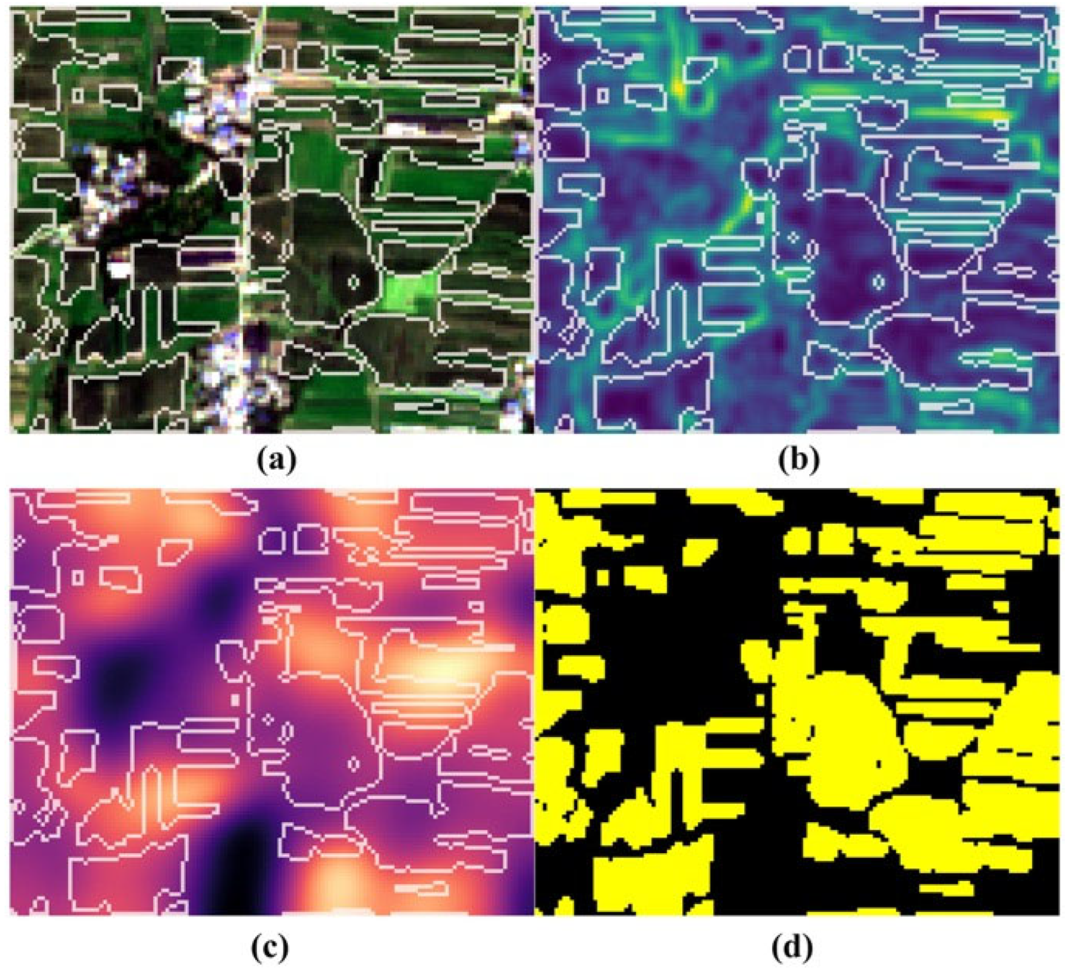
where $f_{DW1}$ and $f_{DW2}$ are two depthwise convolutions, $G_{PW}^{\uparrow }$ and $G_{PW}^{\downarrow }$ are the expansion/reduction PW-Convs, and $\varphi \left(X\right)$ denotes the EW-MHSA branch. LayerNorm/BN and light projection layers can be inserted between branches to stabilize training. Default configuration: DW-Conv kernel $k=3$, stride = 1; PW-Conv reduction ratio $r\in (2,4)$; EW-MHSA window size $w\in \left(7,12\right)$ with shifted windows; activation SiLU or ReLU; Pre-Norm normalization. Compared with global attention, ASL exhibits a more controllable complexity growth, making it well-suited for shallow/mid encoder stages and symmetric placement in the decoder, thereby balancing detail preservation and contextual modeling in high-resolution agricultural scenes. In practice, ASL produces high responses along soybean parcel boundaries and row structures while suppressing noise in homogeneous background regions. As illustrated in Figure 2b, the ASL-enhanced shallow feature map exhibited intensified activations aligned with the red parcel boundaries and crop-row directions, intuitively confirming its role as a boundary- and texture-enhancement module in the shallow encoder–decoder stages.

3.2.2. Parallel Vision Mamba Layer (PVML)

To effectively capture long-range dependencies and ensure semantic consistency across agricultural parcels, we introduced the Parallel Vision Mamba Layer (PVML) for global spatial representation learning [47]. Given that the Mamba architecture is highly sensitive to the channel dimension, an increase in the number of channels substantially enlarges both the state dimension and the projection matrices, leading to rapid growth in parameter count and memory consumption [26,48].

To address this, PVML adopts a lightweight design based on channel-wise parallelization, residual scaling, and projection fusion. Specifically, the input feature $X\in R^{H\times W\times C}$ is first normalized using LayerNorm, then equally divided into four channel groups (each of size $C/4$). These sub-features are independently processed by parallel Mamba-SSM branches, which model long-range dependencies in linear time complexity. The choice of four groups provides a practical balance between per-branch width and parallel diversity: each branch retains sufficient channel capacity to learn expressive dynamics, while the total number of branches remains small enough to keep the overall parameter count and memory footprint close to that of the baseline backbone. The outputs of each branch are subsequently residually scaled and fused through additive or concatenation operations, followed by a linear projection to restore the full C channel dimension and align with the main network (Figure 1b). This design substantially strengthens global contextual perception and cross-parcel semantic coherence while maintaining nearly constant channel and memory budgets. The overall computation can be formulated as follows:

$$Y_i^{C/4}=SP\left[LN(X_{in}^C)\right],i=1,2,3,4$$

(4)

$$VM\_Y_i^{C/4}=Mamba\left(Y_i^{C/4}\right)+\lambda Y_i^{C/4}$$

(5)

$$X_{out}=cat\left(VM\_Y_i^{C/4}\right)$$

(6)

$$Out=Pro\left[LN\left(X_{Out}\right)\right]$$

(7)

where LN denotes Layer Normalization, SP is the Split operation, Mamba is the Mamba operator, $\lambda$ is the residual scaling factor, $Cat$ is the concatenation, and Pro is the linear projection. By processing features through PVML in this manner, the total number of channels remains unchanged, enabling high-precision global representation learning while minimizing parameter overhead and maintaining computational efficiency. Consequently, PVML tends to produce smooth and homogeneous activations within soybean parcels while maintaining sharp transitions at parcel boundaries. As shown in Figure 2c, the PVML-based deep feature map was almost uniform inside the yellow soybean fields and clearly suppressed in surrounding non-soybean areas, providing an intuitive demonstration that PVML improves parcel-level semantic coherence and reduces within-field fragmentation in a way that complements the boundary-focused behavior of ASL. The intermediate feature visualizations in Figure 2b, c therefore offer an intuitive complement to the mathematical formulations of ASL and PVML.

3.2.3. Selective State Space Model (SSM)

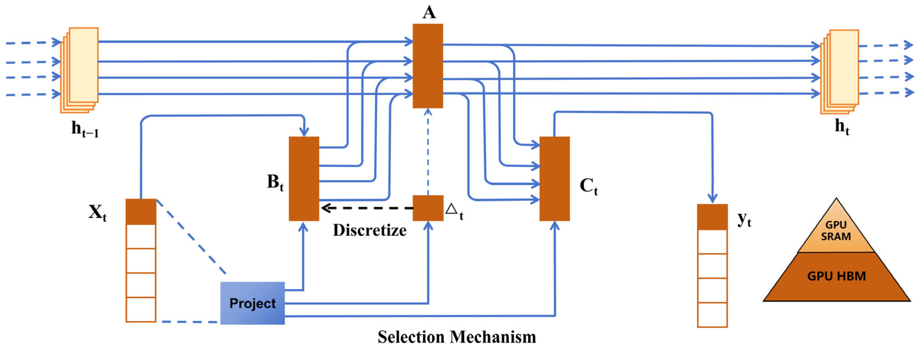
The Mamba module, serving as the core component of APM-UNet, is built upon a Selective State Space Model (SSM) [49]. The SSM follows a fundamental paradigm of state evolution and observation mapping, which efficiently captures long-range dependencies with linear-time complexity. It can be viewed as a unified and extended framework that bridges the temporal modeling capability of recurrent neural networks (RNNs) and the local representation power of convolutional neural networks (CNNs) [50,51]. The continuous-time form of the SSM is expressed as follows:

$$h^{\prime }\left(t\right)=Ah\left(t\right)+Bx\left(t\right)$$

(8)

$$y\left(t\right)=Ch\left(t\right)+Dx\left(t\right)$$

(9)

where Equation (8) represents the state transition, and Equation (9) defines the observation mapping. These two equations jointly constitute the mathematical foundation of the SSM, which aims to infer the latent state variable $h\left(t\right)$ from a given input $x(t)$ and a set of system parameters, thereby establishing a dynamic and interpretable input–output mapping. Here, $A\in R^{N\times N}$ is the state-transition matrix governing interactions among internal states, $B\in R^N$ is the input matrix defining how the external signal $x\left(t\right)$ drives state evolution, $C\in R^N$ is the output (observation) matrix mapping latent states to the observable outputs, and $D\in R^N$ is the direct feed-through term describing direct input–output coupling (commonly set to $D=0$). A schematic representation of the SSM operational mechanism is illustrated in Figure 3.

In the implementation of the Mamba-SSM module, the two-dimensional feature maps are first serialized following a predefined scanning strategy (e.g., row-wise, column-wise, or selective multi-directional scanning). These serialized sequences are then fed into the Mamba-SSM, which models long-range dependencies and captures global contextual information with linear time complexity. The resulting representations are subsequently aligned and fused with outputs from the local convolutional and window-based attention branches through a gated residual fusion mechanism, achieving an optimal balance between boundary fidelity and cross-parcel semantic consistency. This design significantly improves the accuracy, robustness, and generalization performance of soybean mapping in high-resolution remote sensing imagery, while maintaining nearly constant parameter count and memory consumption.

3.3. Accuracy Evaluation Methods

To comprehensively assess the performance of the proposed network in remote sensing imagery classification and segmentation tasks, six quantitative metrics were employed: Producer’s Accuracy (PA), Overall Accuracy (OA), Kappa coefficient (Kappa), Recall, Intersection over Union (IoU), and the F1-score (F1). Unless otherwise specified, all metrics were computed at the pixel level, and the final scores are reported as macro-averages across all classes to ensure class-balanced evaluation. The corresponding mathematical formulations are as follows:

$$PA={\displaystyle \frac{TP}{TP+FP}}$$

(10)

$$OA={\displaystyle \frac{{\displaystyle \sum TP}}{{\displaystyle \sum \left(TP+FN+FP+TN\right)}}}$$

(11)

$$Kappa={\displaystyle \frac{OA-PE}{1-PE}}$$

(12)

$$Recall={\displaystyle \frac{TP}{TP+FN}}$$

(13)

$$IoU={\displaystyle \frac{TP}{TP+FP+FN}}$$

(14)

$$F1=2\times {\displaystyle \frac{PA\times Recall}{PA+Recall}}$$

(15)

where TP (True Positives) denotes the number of pixels correctly classified as the target class, FP (False Positives) refers to the number of non-target pixels incorrectly predicted as the target class, and FN (False Negatives) represents the number of target pixels that were not correctly identified by the model. Additionally, the Producer’s Accuracy Weighted Average (PE) is calculated by applying predefined class weights to individual PA values to account for category imbalance and to better reflect the model’s class-specific reliability.

3.4. Experimental Setup and Training Strategy

All experiments were conducted on an NVIDIA GeForce RTX 4090 GPU under Ubuntu 20.04, with CUDA 11.3 and cuDNN 8.2.1 configured for GPU acceleration. The deep learning framework used was PyTorch v1.8.1. To ensure reproducibility, random seeds were fixed and deterministic operations were enabled. The input comprised multi-temporal Sentinel-1/2 fused data, with each spectral and polarization channel normalized using z-score standardization. The imagery was partitioned into 512 × 512 training patches (stride = 256 px) to enhance spatial coverage and boundary utilization, with stratified sampling adopted to balance class distribution and spatial heterogeneity. Data augmentation included random rotation and flipping, scale perturbation, random cropping, and mild spectral and speckle noise injection. On the output side, label smoothing ($\epsilon =0.05$) was applied to mitigate overfitting and improve generalization. The network was trained end-to-end with a mini-batch size of 16 patches using a compound loss that combined class-balanced cross-entropy and Dice loss with equal weighting. Specifically, the total loss is defined as:

$$L=L_{CBCE}+L_{Dice}$$

(16)

$$L_{Dice}=-Dice$$

(17)

So that lower (and possibly negative) values of L correspond to better agreement between predictions and reference labels. Model optimization was performed using stochastic gradient descent (SGD) with a momentum of 0.9 and the following key hyperparameters: an initial learning rate of 0.0006, weight decay of 0.00025, and 2000 training epochs. To prevent overfitting and accelerate convergence, an early stopping mechanism was adopted: training was terminated if the validation loss failed to decrease for 100 consecutive epochs. Additionally, a learning-rate decay schedule was applied—when the validation loss plateaued for three consecutive epochs, the learning rate was halved. Experimental results demonstrate that the proposed approach achieved high convergence efficiency and training stability in soybean mapping tasks based on multi-temporal remote sensing imagery.

4. Results and Analysis

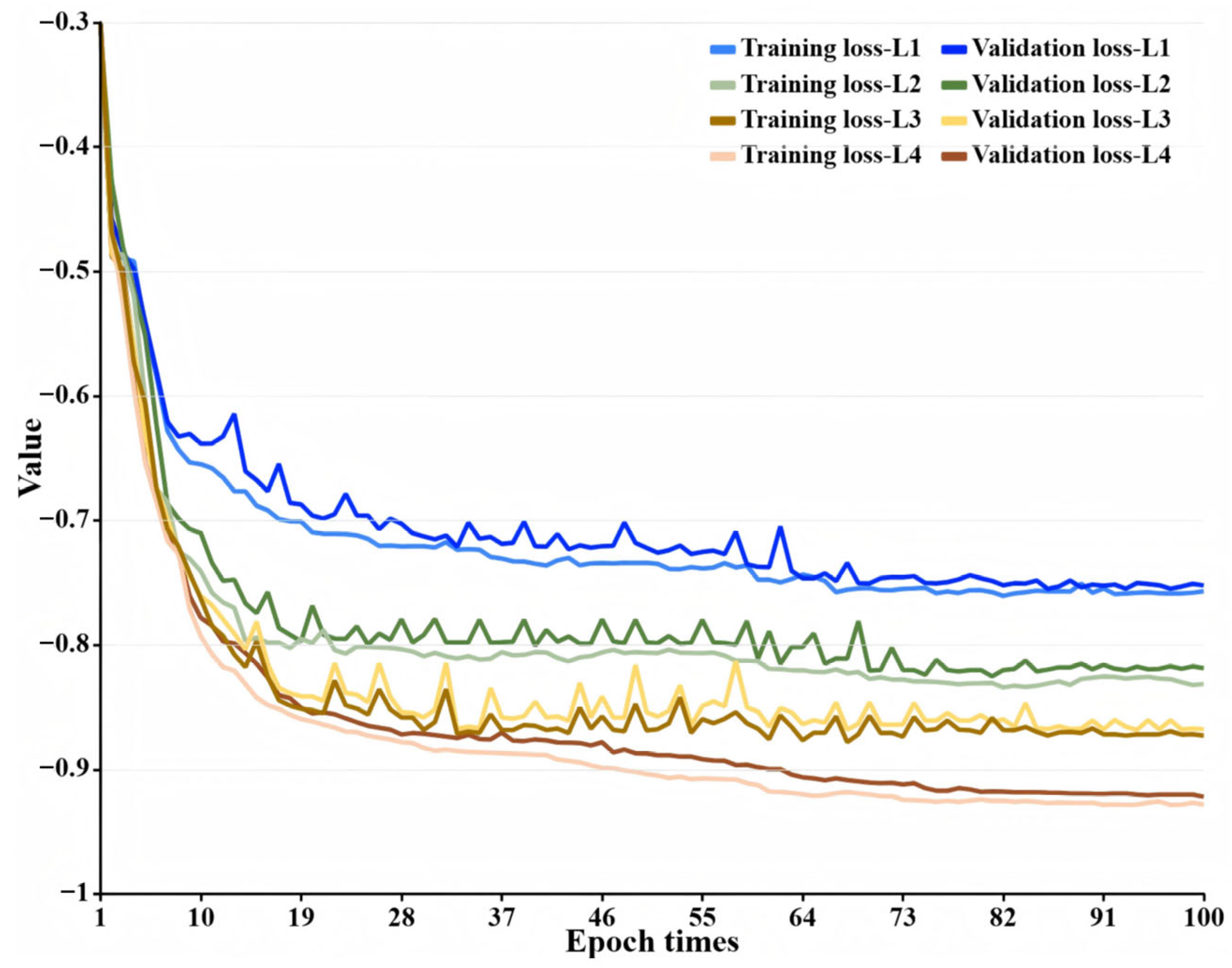
4.1. Network Training and Loss Evolution

To verify the convergence behavior, parameter optimization efficiency, and the influence of different feature subsets, the APM-UNet model was trained iteratively on soybean samples from Biyang County, with the validation set continuously monitored to evaluate generalization performance. The training and validation loss curves for the four feature configurations (L1–L4) as a function of training epoch are shown in Figure 4. Across all configurations, both curves exhibited a coherent three-stage evolution. During the early phase, the loss decreased rapidly within the first ten epochs, indicating that the model effectively learned the mapping between features and class labels through fast gradient adjustment. In the subsequent phase (approximately 10–35 epochs), the decline slowed as the network entered parameter fine-tuning and stability adjustment. After about 35 epochs, the losses of both training and validation sets reached a steady plateau, and the gap between them remained small (≤0.05) without the characteristic divergence in which training loss continues to decrease while validation loss increases, indicating stable convergence without evident overfitting under the adopted training protocol. This stable convergence pattern highlights the complementary strengths of the APM-UNet architecture: the U-Net backbone enhances local texture and boundary representation, while the Mamba-SSM module captures long-range spatial dependencies, jointly improving representational integrity while mitigating noise-induced overfitting. Among the four feature groups, L4 achieved the lowest validation loss throughout training, stabilizing around −0.92 under the above loss definition, where the negative value reflects the dominance of the negative Dice term when segmentation quality is high, representing improvements of 22.7%, 10.8%, and 5.7% compared with L1 (−0.75), L2 (−0.83), and L3 (−0.87), respectively. This superior performance results from the JM-based “filter-then-learn” strategy, which removes redundant variables while retaining highly discriminative features (such as EVI and NDWI from the pod-filling phase). The resulting compact, physically interpretable subset reduces model complexity and accelerates convergence, making L4 the optimal configuration for subsequent classification experiments. Throughout training, the application of stochastic gradient descent (SGD), learning-rate decay, and early stopping strategies further enhanced convergence efficiency and stability, demonstrating that the proposed APM-UNet framework maintains reliable optimization behavior in large-scale soybean mapping scenarios.

4.2. JM Distance–Based Feature Selection Results

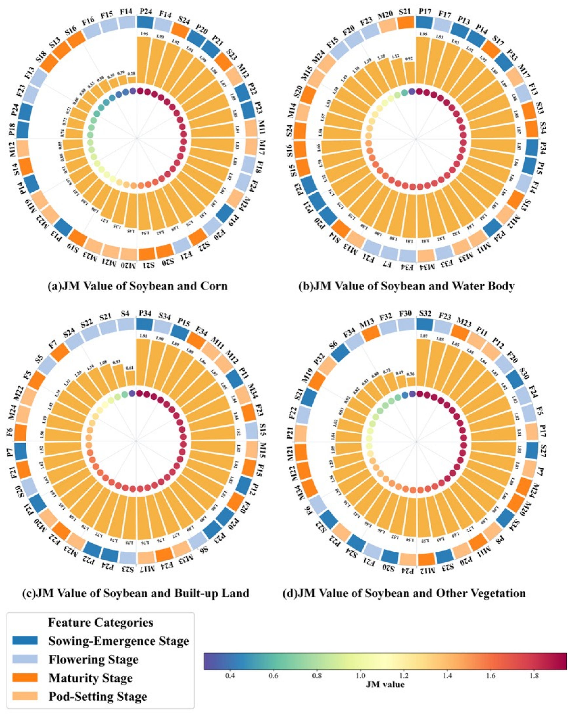
A total of 136 candidate features were comprehensively analyzed in this study, encompassing four categories: original spectral bands, vegetation indices, texture features, and polarization parameters. For each of the four key temporal phases, the Jeffries–Matusita (JM) distance between the soybean and non-soybean classes was computed using Equation (1), yielding separability values for four class pairs. As illustrated in Figure 5, the enrichment map visualizes the JM distance distribution across temporal phases and feature types, effectively revealing the inter-class separability patterns under different phenological and data-fusion conditions. This visualization highlights how specific temporal–spectral–polarization combinations contribute to class discrimination, thereby providing a quantitative and physically interpretable basis for feature selection in the subsequent crop-type classification process.

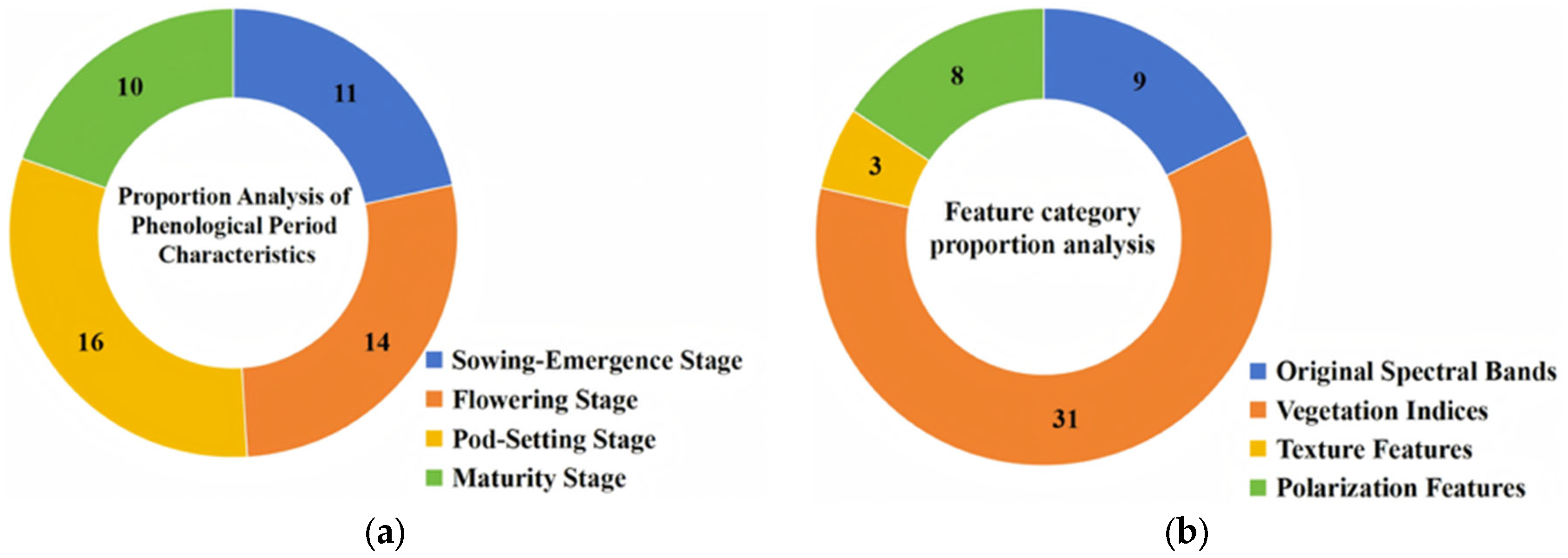
Through the JM distance-based feature selection algorithm, a total of 51 features with a maximum JM value ≥ 1.8 were retained to construct the optimal feature subset (feature set D4). As shown in Figure 6a, the phenological-phase distribution of these features indicates that the Pod-Setting Stage contributed the largest proportion, with 16 features, underscoring its dominant discriminative role during this key growth period. From the perspective of feature-type composition (Figure 6b), vegetation indices accounted for the largest share, with 39 features, highlighting their strong ability to capture canopy spectral variation and vegetation vigor. Overall, the JM-based selection results demonstrate that Pod-Setting Stage observations and vegetation-index–derived features jointly made the most substantial contribution to the optimized subset. Their synergistic effect enhances the separability and robustness of soybean mapping, providing a critical spectral–temporal basis for the accurate delineation of soybean cultivation areas. The detailed list of the 51 JM-selected features, including their phenological stages, feature types, JM values, and rankings, is provided in

Table 4. Final JM-selected multi-source, multi-temporal features.

Rank	Feature Code	Feature Name	Phenological Stage	Feature Type	JM Value
1	S6	B7	Sowing-Emergence Stage	Original Spectral Band	1.80
2	S13	NDVI	Sowing-Emergence Stage	Vegetation Indices	1.85
3	S15	RVI	Sowing-Emergence Stage	Vegetation Indices	1.82
4	S17	NDWI	Sowing-Emergence Stage	Vegetation Indices	1.92
5	S23	NDre2	Sowing-Emergence Stage	Vegetation Indices	1.88
6	S24	CIre	Sowing-Emergence Stage	Vegetation Indices	1.92
7	S27	Entropy	Sowing-Emergence Stage	Texture Features	1.81
8	S30	Dissimilarity	Sowing-Emergence Stage	Texture Features	1.82
9	S32	Contrast	Sowing-Emergence Stage	Texture Features	1.87
10	S33	VV	Sowing-Emergence Stage	Polarization Features	1.88
11	S34	VH	Sowing-Emergence Stage	Polarization Features	1.90
12	F5	B7	Flowering Stage	Original Spectral Band	1.82
13	F7	B8	Flowering Stage	Original Spectral Band	1.80
14	F13	NDVI	Flowering Stage	Vegetation Indices	1.88
15	F14	EVI	Flowering Stage	Vegetation Indices	1.93
16	F15	RVI	Flowering Stage	Vegetation Indices	1.82
17	F17	NDWI	Flowering Stage	Vegetation Indices	1.93
18	F18	SAVI	Flowering Stage	Vegetation Indices	1.83
19	F20	NDVIre2	Flowering Stage	Vegetation Indices	1.81
20	F20	NDVIre2	Flowering Stage	Vegetation Indices	1.83
21	F21	NDVIre3	Flowering Stage	Vegetation Indices	1.80
22	F23	NDre2	Flowering Stage	Vegetation Indices	1.85
23	F24	CIre	Flowering Stage	Vegetation Indices	1.82
24	F33	VV	Flowering Stage	Polarization Features	1.82
25	F34	VH	Flowering Stage	Polarization Features	1.89
26	P7	B8	Pod-Setting Stage	Original Spectral Band	1.81
27	P8	B8A	Pod-Setting Stage	Original Spectral Band	1.80
28	P11	B11	Pod-Setting Stage	Original Spectral Band	1.85
29	P12	B12	Pod-Setting Stage	Original Spectral Band	1.84
30	P13	NDVI	Pod-Setting Stage	Vegetation Indices	1.93
31	P14	EVI	Pod-Setting Stage	Vegetation Indices	1.92
32	P15	RVI	Pod-Setting Stage	Vegetation Indices	1.89
33	P17	NDWI	Pod-Setting Stage	Vegetation Indices	1.95
34	P19	NDVIre1	Pod-Setting Stage	Vegetation Indices	1.81
35	P20	NDVIre2	Pod-Setting Stage	Vegetation Indices	1.91
36	P21	NDVIre3	Pod-Setting Stage	Vegetation Indices	1.90
37	P22	NDre1	Pod-Setting Stage	Vegetation Indices	1.85
38	P23	NDre2	Pod-Setting Stage	Vegetation Indices	1.85
39	P24	CIre	Pod-Setting Stage	Vegetation Indices	1.95
40	P33	VV	Pod-Setting Stage	Polarization Features	1.89
41	P34	VH	Pod-Setting Stage	Polarization Features	1.91
42	M11	B11	Maturity Stage	Original Spectral Band	1.86
43	M12	B12	Maturity Stage	Original Spectral Band	1.87
44	M13	NDVI	Maturity Stage	Vegetation Indices	1.8
45	M15	RVI	Maturity Stage	Vegetation Indices	1.82
46	M17	NDWI	Maturity Stage	Vegetation Indices	1.89
47	M20	NDVIre2	Maturity Stage	Vegetation Indices	1.8
48	M23	NDre2	Maturity Stage	Vegetation Indices	1.85
49	M24	CIre	Maturity Stage	Vegetation Indices	1.81
50	M33	VV	Maturity Stage	Polarization Features	1.82
51	M34	VH	Maturity Stage	Polarization Features	1.84

.

4.3. Classification Results

To rigorously assess the efficacy of JM distance-based feature selection for dimensionality reduction, redundancy suppression, and computational economy—and to evaluate the feasibility and advantages of APM-UNet for soybean mapping—we benchmarked against three representative paradigms: U-Net (convolutional), SegFormer (Transformer), and Vision-Mamba (state-space/Mamba). All models were reproduced under identical preprocessing, input modalities (Sentinel-1/2 and their fusion), training schedules, and evaluation protocols, and were contrasted at comparable parameter counts and compute budgets with respect to classification accuracy, boundary consistency, and inference efficiency.

To disentangle temporal–modal contributions while keeping notation compact, four feature configurations were considered: all features across four phenological phases (136 features, D1), the single-window Sentinel-1/2 dataset at the Pod-Setting Stage (34 features, D2), the JM-filtered optical subset (44 features, D3), and the JM-filtered multi-source, multi-temporal subset (51 features, D4). Crossing the four networks with these four configurations yielded 16 experimental settings (see

Table 5. Classification experiment combination information table.

Feature Set ID	Number of Features	Unet	SegFormer	Vision-Mamba	APM-UNet
D1	136	U1	S1	V1	AU1
D2	34	U2	S2	V2	AU2
D3	44	U3	S3	V3	AU3
D4	51	U4	S4	V4	AU4

for the unified naming), enabling a protocol-consistent comparison across architectures and an explicit quantification of the marginal gains attributable to the JM-guided feature–phase joint selection.

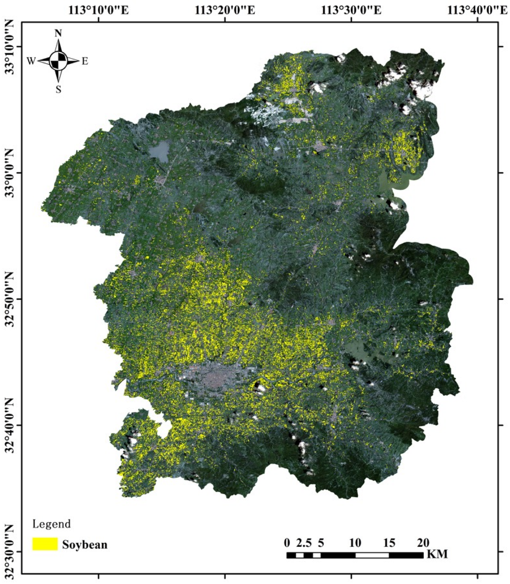
As shown in Figure 7, a spatial and holistic comparison across sixteen configurations indicates that the JM distance–filtered multi-source, multi-temporal feature set (D4) yielded the best performance for all network architectures. It is worth noting that this improvement did not follow a monotonic trend with feature dimensionality: the unfiltered full set D1 (136 features) performed worse than the more compact JM-selected set D4 (52 features), and the optical-only subset D3 (44 features) remained inferior to D4 despite a similar channel budget, indicating that the gains mainly arise from the JM-based screening of discriminative, phenology-aware features rather than simply increasing the number of channels. Relative to U-Net, SegFormer, and Vision-Mamba, APM-UNet with D4 achieved superior boundary completeness, connectivity of fragmented soybean parcels, and accuracy under heterogeneous backgrounds (forest–farmland mosaics and irrigation networks). In contrast, the unfiltered full set (D1) exhibited substantial redundancy and inter-feature correlation, inducing salt-and-pepper artifacts over bare soil and high-reflectance targets and increasing confusion with co-season crops (e.g., maize, sorghum). The single-temporal set (D2) lacked phenological context and thus inconsistently separated canopy structural differences, whereas the optical subset (D3)—despite better spectral separability than D1 and D2—omitted radar polarization and temporal constraints, leading to blurred boundaries in moist-soil and shadow-transition regions. To demonstrate scalability, Figure 8 presents county-wide soybean mapping over Biyang, where the model maintained high class purity and boundary continuity in complex landscapes, underscoring the robustness of multi-source, multi-temporal features and the local–global collaborative architecture. Overall, D4 retained highly discriminative cues—notably EVI and NDWI from the Pod-Setting Stage and NDVIrel from the Regreening Stage—while fusing optical and radar time series, thereby markedly enhancing generalization and spatial consistency.

To thoroughly evaluate the performance advantages of the proposed algorithm for soybean-planting area extraction, multiple quantitative assessment metrics were employed, as summarized in Table 5. The results consistently demonstrate that the JM-distance-based joint selection of features and phenological windows significantly outperformed both the all-feature and single-window subsets, achieving stable gains across PA, OA, Kappa, IoU, Recall, and F1 metrics. Notably, under identical feature configurations, APM-UNet exhibited a consistently superior overall performance compared with U-Net, SegFormer, and Vision-Mamba, highlighting the complementary advantages of the Attention Sandglass Layer (ASL)—which enhances shallow-level local texture and boundary sensitivity—and the Parallel Vision Mamba Layer (PVML/Mamba-SSM)—which strengthens long-range dependency and global consistency in deeper representations. For the optimal configuration (AU4), the model achieved PA = 92.81%, OA = 97.95%, Kappa = 0.9649, Recall = 91.42%, IoU = 0.7986, and F1 = 0.9324, representing improvements of approximately 7.5 and 6.2 percentage points in PA and OA, respectively, compared with its all-feature counterpart. In terms of feature contributions, the multi-source scheme incorporating Sentinel-1 polarizations (VV/VH) outperformed optical-only inputs, indicating that the radar backscattering mechanism enhances robustness against cloud-shadow interference and landscape fragmentation, thereby improving cross-parcel semantic consistency. Conversely, single-window feature subsets failed to ensure stable discrimination under complex cropping structures and frequent cloud coverage. In contrast, the multi-temporal, multi-source JM-distance-based feature selection effectively compressed redundancy while amplifying inter-class temporal differences. Overall, the trends observed in

Table 6. Classification accuracy of different experimental combination methods.

Experimental Combination	PA (%)	OA (%)	Kappa	Recall (%)	IoU
U1	82.56	85.53	0.7992	82.32	0.6413
U2	70.64	74.38	0.7038	70.65	0.5443
U3	83.18	87.71	0.8393	83.28	0.6563
U4	86.27	90.16	0.8457	84.42	0.6704
S1	84.29	89.27	0.8217	83.55	0.6778
S2	72.16	77.17	0.7194	72.76	0.5711
S3	85.08	88.09	0.8551	85.14	0.6833
S4	88.53	93.38	0.8855	87.88	0.7604
V1	83.34	86.77	0.8164	83.51	0.6631
V2	72.03	75.86	0.7084	72.19	0.5593
V3	84.88	87.82	0.8513	84.99	0.6794
V4	87.35	91.97	0.8803	87.59	0.7148
AU1	85.34	91.74	0.8768	85.87	0.6891
AU2	74.65	80.69	0.7532	76.72	0.6048
AU3	88.57	94.06	0.8765	88.23	0.7348
AU4	92.81	97.95	0.9649	91.42	0.7986

corroborate the qualitative interpretation: the coupling of the JM-distance feature selection algorithm with APM-UNet achieved a superior balance among accuracy, efficiency, and robustness.

4.4. Ablation Study and Computational Efficiency

To comprehensively assess the marginal contributions of the core components within the APM-UNet architecture to segmentation accuracy and computational efficiency, a series of controlled ablation experiments were conducted. In this framework, the Parallel Vision Mamba Layer (PVML) and the Attention Sandglass Layer (ASL) are deeply integrated, serving complementary roles: the PVML models long-range dependencies and global contextual interactions through channel-grouped parallel state-space updates, while the ASL enhances local texture representation and boundary refinement by combining depthwise separable convolution with window-based attention.

Under identical data preprocessing, input modalities, and training/evaluation protocols, only the internal network architecture was modified to generate four comparable configurations. The baseline model retained the original U-Net backbone; the PVML configuration removed the ASL; the ASL configuration excluded the PVML; and the full model incorporated both modules. To ensure fair comparison, the number of parameters and GFLOPs were maintained at approximately the same level, thereby isolating and quantifying the independent and joint effects of the two components.

As summarized in

Table 7. Results of the Ablation Study. In the experiments, “√” denotes that the module is enabled (used), whereas “×” indicates it is disabled (not used).

ASL	PVML	Param (M)	GFLOPs	PA (%)	OA (%)	Kappa	Recall	IoU	F1
×	×	11.8	47.3	82.61	85.52	0.7991	82.34	0.6415	0.8212
×	√	12.1	49.2	84.73	92.01	0.8802	87.65	0.7153	0.8692
√	×	12.0	48.8	87.24	93.31	0.8862	88.09	0.7603	0.8741
√	√	12.5	50.2	92.81	97.95	0.9649	91.42	0.7986	0.9324

, the PVML configuration exhibited clear improvements in IoU and F1 relative to the baseline, confirming that long-range modeling effectively enhanced semantic coherence across spatially fragmented regions, although minor boundary adhesion and local discontinuities remained. The ASL configuration further improved IoU, F1, and PA, with corresponding increases in OA and Kappa, demonstrating its ability to preserve fine-scale texture and boundary fidelity. Within the soybean-mapping experiments conducted for Biyang County in 2023, these trends are consistent across all tested feature configurations, but the marginal benefits of ASL and PVML have not yet been systematically evaluated on independent regions, seasons, or crop types. When both components operated jointly, the full model achieved the highest performance across all metrics, revealing a distinct local–global complementarity: the ASL refines boundaries and detail discrimination, while the PVML introduces long-range feature interaction and inter-parcel consistency through channel grouping, residual scaling, and lightweight projection. With only a marginal increase in computational complexity, the full configuration yielded simultaneous gains in OA, Kappa, Recall, IoU, and F1, indicating an optimal trade-off between accuracy and efficiency.

To further assess practical deployability, we compared the inference speed and memory consumption of APM-UNet with the three baseline networks (U-Net, SegFormer, and Vision-Mamba) under identical hardware and software settings. All models were evaluated on an NVIDIA GeForce RTX 4090 GPU with batch size = 1 and an input patch size of 512 × 512 pixels, using the same PyTorch environment described in Section 3.4. For each model, the average inference time per tile was computed over multiple forward passes after a warm-up phase (excluding data loading), and the peak GPU memory usage was recorded with PyTorch profiling tools. As reported in

Table 8. Inference efficiency comparison of APM-UNet and baseline models on an NVIDIA RTX 4090 GPU (batch size = 1, input size = 512 × 512).

Model	Param (M)	GFLOPs	Inference Time (ms/Tile)	Throughput (Tiles/s)	Peak GPU Memory (GB)
UNet	11.8	47.3	11.8	84.7	2.1
SegFormer	13.5	76.3	18.9	52.9	3.8
Vision-Mamba	15.8	82.4	20.4	49.0	4.1
APM-UNet	12.5	50.2	10.5	95.2	2.3

, APM-UNet attained competitive or faster inference speed than U-Net and clearly outperformed the Transformer-based SegFormer and Vision-Mamba in terms of latency, while requiring a memory footprint comparable to U-Net and substantially lower than that of the Transformer baselines. Overall, these results indicate that APM-UNet not only improves segmentation accuracy but also maintains a computational profile that is well suited to large-area and near-real-time soybean mapping applications.

5. Discussion

5.1. Comparative Analysis of Feature Selection Methods

Under unified data preprocessing and training protocols, four types of feature sets were constructed and systematically compared across four representative architectures—U-Net, SegFormer, Vision-Mamba, and APM-UNet—to evaluate the influence of feature construction on classification performance. Feature selection employed a Jeffries–Matusita (JM) distance-based filtering strategy, which simultaneously assessed global separability and inter-channel correlation while incorporating class-specific local separability to prevent the masking of key inter-class differences by global averaging. With a threshold of JM > 1.8, a total of 51 optimal features were retained, and their temporal (month-wise) and categorical distributions were analyzed to trace the sources of discriminative power. The Pod-Setting Stage contributed the largest number of selected features, vegetation indices dominated in feature type, and all Sentinel-1 VV/VH polarization features were retained, underscoring the complementarity between optical and radar modalities. To quantify the marginal contribution of temporal information, a single-phase control group (Pod-Setting Stage only) was designed and compared against multi-temporal feature sets under identical network conditions.

Quantitative evaluations demonstrated that JM-based optimization consistently produced stable and significant improvements across all networks, outperforming both “full-feature” and “single-phase/single-source” schemes. For example, in U-Net, JM optimization (U4) increased OA from 85.53% to 90.16%, IoU from 0.6413 to 0.6704, and F1 from 0.8306 to 0.8451, indicating that enhanced feature separability can systematically improve both pixel-level and boundary-level precision without increasing model complexity. Similar patterns were observed across architectures: JM-optimized configurations (S4, V4, AU4) achieved superior PA, OA, Kappa, IoU, and F1 scores compared to their respective baselines, with AU4 achieving the best overall performance (PA 92.81%, OA 97.95%, Kappa 0.9649, Recall 91.42%, IoU 0.7986, F1 0.9324). Furthermore, multi-temporal features consistently outperformed single-phase inputs, confirming that phenological diversity effectively amplifies inter-class separability.

Mechanistically, the JM-driven filtering criterion, combined with thresholding and correlation constraints, produced a compact yet complementary feature subset that simultaneously emphasized phenological variations and electromagnetic scattering differences among crop types in a multi-source, multi-temporal representation space. This synergy led to concurrent gains in boundary-sensitive metrics (IoU, F1) and overall consistency metrics (OA, Kappa). Contribution analysis revealed that red-edge and water-sensitive vegetation indices enhanced the spectral representation of canopy physiological–structural differences, thereby improving the classification of fragmented parcels and forest–farmland transition zones; meanwhile, Sentinel-1 VV/VH polarization features, complementary to optical spectra, maintained robust discrimination under cloud shadow and speckle interference, enhancing cross-parcel semantic consistency.

In summary, the integration of multi-source (Sentinel-1/2) and multi-temporal data with JM-distance-based feature filtering achieves fine-grained boundary delineation and global spatial consistency without adding computational complexity. This strategy complements the ASL (local feature enhancement) and PVML/SSM (global semantic modeling) modules of APM-UNet, jointly supporting the model’s superior balance among accuracy, boundary fidelity, and spatial consistency. Consequently, the JM-optimized composite feature set is established as the recommended configuration for subsequent experiments and practical applications in multi-temporal remote sensing crop classification.

5.2. Multi-Source Data Analysis

Under ensured experimental comparability, this section evaluates the marginal contributions of data sources (Sentinel-1/2) and temporal information (multi-temporal vs. single-temporal) to classification performance, with mechanistic interpretations supported by JM-distance-based feature selection results. (1) Multi-source fusion outperformed single-source configurations. The complementary imaging mechanisms of optical and SAR data effectively mitigate interference from shadows, thin clouds, and complex background textures, yielding a systematic improvement in OA and Kappa, while substantially enhancing spatial consistency and patch integrity within fragmented parcels and forest–farmland transition zones (see Figure 6). This advantage is consistently observed across all architectures (U-Net, SegFormer, Vision-Mamba, and APM-UNet), indicating that the benefits of multi-source fusion are architecture-independent. (2) Multi-temporal data outperformed single-phase inputs, with improvements reflected simultaneously in boundary-sensitive metrics (IoU, F1) and overall consistency metrics (OA, Kappa). Phenological variations amplify class separability along the temporal dimension, particularly in narrow plots, mosaic landscapes, and high-texture regions. Consistent with this finding, JM-based phenological contributions show that the Pod-Setting and Flowering stages exhibited the highest weights (approximately 32.69% and 26.92%, respectively), aligning with regional agricultural practices and phenological rhythms: early spring wilting/regreening and early summer cultivation/growth transitions enhance spectral and scattering contrast between target and non-target classes, thereby improving temporal discriminability.

From the perspective of feature-type contributions, the JM-optimized subset demonstrated a structural preference for spectral/physiological and radar-scattering features while de-emphasizing texture-based descriptors. Vegetation indices dominated (approximately 75%), with red-edge and water-sensitive indices effectively magnifying cross-phenological canopy physiological–structural differences. Following these were Sentinel-1 VV/VH polarization parameters and original optical bands: the former complements optical information through dielectric constant and surface roughness dimensions, effectively mitigating “voids” and cross-parcel adhesion within large-field and strip-shaped landscapes; the latter provides a stable spectral baseline for class discrimination. Texture features, in contrast, were minimally selected due to strong correlations with multi-temporal indices and because JM metrics at the pixel level preferentially retain spectral/polarimetric dimensions that directly enlarge inter-class separability. Overall, JM-distance-based feature optimization, guided by the principle of maximizing inter-class distance while minimizing intra-class variance, preserves compact, low-redundancy, and information-rich variables that emphasize physiological and scattering characteristics. This enables concurrent improvements in boundary-sensitive metrics (IoU, F1) and overall consistency metrics (OA, Kappa) without substantially increasing model complexity.

In summary, the integration of multi-source (Sentinel-1/2) and multi-temporal data with JM-distance-based optimization establishes a data–feature synergy: the former provides modal complementarity and phenological amplification, while the latter suppresses redundancy and correlation interference. Their combined effect enables all architectures—especially APM-UNet—to achieve concurrent gains in quantitative metrics (PA, OA, Kappa, Recall, IoU, F1) and qualitative performance (boundary continuity, patch integrity, and cross-parcel consistency), thus providing a robust foundation for regional scalability and long-term temporal monitoring in agricultural remote sensing applications.

5.3. Comparative Analysis of Classification Methods

The superior performance of APM-UNet under multi-temporal Sentinel-1/2 fusion can be attributed to the synergy between its local–global collaborative modeling and feature–phenology joint optimization strategies. The shallow Attention Sandglass Layer (ASL) enhances edge discrimination and fine-grained texture perception, while the mid-to-deep Parallel Vision Mamba Layer (PVML) (based on the Mamba State Space Model) captures long-range dependencies and cross-parcel semantic consistency with near-linear computational complexity. This dual mechanism effectively alleviates the under-segmentation of small parcels typical of U-Net and over-segmentation of large parcels observed in SegFormer, thereby leading to simultaneous improvements in boundary-sensitive metrics (IoU, F1) and global-consistency metrics (OA, Kappa). Complementarily, the D4 multi-source and multi-temporal feature subset, constructed via JM-distance-based joint selection, provides a low-redundancy and highly separable input space: Sentinel-1 VV/VH polarizations offer scattering robustness that suppresses salt-and-pepper noise caused by clouds or highly reflective surfaces, while Sentinel-2 red-edge and water-sensitive indices describe canopy physiological–structural dynamics and moisture conditions. Their temporal complementarity significantly enhances the model’s spatial fidelity and classification stability across fragmented landscapes and mixed backgrounds (e.g., forest–farmland ecotones, irrigation networks). Quantitatively, APM-UNet achieved a PA 90.73%, OA 96.21%, Kappa 0.945, Recall 91.58%, IoU 0.81, and F1 0.92, outperforming Vision-Mamba by approximately 2.8 percentage points and 0.024, and yielding visibly sharper boundaries and higher patch connectivity (Figure 6; Table 5). Overall, the integrated ASL + PVML × D4 (select-then-learn) paradigm attained a refined balance among accuracy, spatial continuity, and computational efficiency, demonstrating strong potential for within-season updates and large-scale mapping. Nevertheless, the model’s performance remains sensitive to temporal quality, cross-sensor co-registration, and class imbalance; extreme cloud contamination, temporal gaps, or substantial S1/S2 misalignment may degrade boundary sharpness and connectivity, while imbalance can suppress minority-class recall. Future work should focus on adaptive temporal weighting/gating, domain adaptation and cross-regional transfer, and joint regularization of boundary consistency and uncertainty (e.g., energy-functional or Kalman-based confidence propagation), while exploring lightweight coupling with differentiable contour or level-set layers to further improve boundary expressiveness, reliability, and inference robustness without significant increases in model complexity.

In relation to existing soybean-mapping studies, these findings highlight three specific advances of the proposed framework. First, compared with traditional approaches that rely on single-source optical imagery and heuristic feature sets or generic feature-ranking schemes, the JM-guided, phenology-aware pre-filtering in APM-UNet produces a compact and physically interpretable multi-source feature subset while still achieving state-of-the-art accuracy, thereby reducing redundancy and mitigating overfitting in fragmented landscapes. Second, relative to mainstream CNN- and Transformer-based segmentation networks reported in the literature, which typically improve accuracy at the cost of substantially higher parameter counts and quadratic self-attention complexity, the combination of ASL and PVML/Mamba in APM-UNet attains competitive or superior IoU and F1 with comparable model size and near-linear computational complexity, offering a more practical balance between accuracy and efficiency for large-area crop mapping. Third, whereas many previous works are constrained to single-phase or single-sensor configurations, our explicit integration of multi-temporal Sentinel-2 spectral–index information with Sentinel-1 VV/VH backscatter demonstrates clear gains in boundary fidelity, parcel connectivity, and minority-class recall, underscoring the value of a “filter-then-learn” design that jointly optimizes data, features, and architecture for operational soybean monitoring.

5.4. Regional Pattern and Driving Mechanisms

As revealed by the county-wide map in Figure 8, soybean cultivation is markedly concentrated in the southwestern sector of Biyang County. This pattern emerges from the joint action of topography–soil–irrigation/drainage and industrial–institutional drivers: flatter terrain, gentle slopes, and well-drained soils favor stable mechanization; concentrations of high-standard farmland with regular parcel geometry and dense canal/field-road networks reduce unit operating costs; compared with flood-prone zones, the southwest shows lower waterlogging risk and smaller inter-annual variability, making yields and returns more predictable; denser cooperatives and storage facilities shorten transport distances and strengthen market pull; and long-term rotations (e.g., with maize) utilize soybean biological nitrogen fixation, reinforcing path dependence and diffusion effects. In terms of area consistency, the official soybean area is 29.62 ha, while our algorithm estimates 28.95 ha, i.e., an absolute difference of 0.67 ha (2.26%), indicating close agreement. Methodologically, the APM-UNet × D4 setting (JM-selected multi-source, multi-temporal features) is robust at both local and global scales: as quantified in Table 6, the D4 configurations (U4, S4, V4, AU4) achieved the highest OA, IoU and F1 among the four feature sets (D1–D4) for all three backbone networks—for example, in U-Net, JM optimization increases OA from 85.53% (U1) to 90.16% (U4) and IoU from 0.6413 to 0.6704, while AU4 attained a PA = 92.81%, OA = 97.95%, IoU = 0.7986 and F1 = 0.9324—indicating that D4 retains highly discriminative phenological and polarization cues while suppressing redundancy and inter-feature correlation, and thus empirically outperforms D1/D2/D3 across models; the ASL × PVML/SSM synergy enhances boundary continuity, parcel integrity, and cross-parcel consistency, which substantiates the spatial coherence and semantic purity observed in the full-coverage map (consistent with Figure 7 and Table 6). For broader deployment, we note potential sensitivities: severe cloud contamination or minor S1/S2 misregistration may affect local boundary coherence, while phenological spectral similarity and class imbalance can induce localized confusion; these can be further mitigated under the filter-then-learn paradigm (JM-based pre-filtering) combined with temporal weighting/gating. Overall, the spatial continuity, boundary fidelity, and reliable area estimation achieved by APM-UNet × D4 provide a transferable pathway for county-scale acreage verification, subsidy auditing, and crop-structure monitoring.

6. Conclusions

This study proposed APM-UNet, a lightweight and interpretable segmentation framework that couples JM-distance–guided feature selection with an attention-enhanced encoder–decoder for high-resolution soybean mapping from multi-temporal Sentinel-1/2 data. Under a unified evaluation protocol, the framework achieved field-scale soybean maps with overall accuracy close to 98% and F1 scores above 0.93, consistently outperforming U-Net, SegFormer and Vision-Mamba, and confirming the effectiveness of the proposed “filter-then-learn” strategy.

Methodologically, APM-UNet was designed with generalizability and efficiency in mind. JM-based pre-filtering compresses the original feature space into a compact, physically interpretable subset that preserves stable class separability while reducing redundancy and parameter count, which is expected to facilitate transfer to other crops, seasons and sensor configurations under similar data conditions. The use of state-space modules with near-linear complexity, instead of quadratic-cost attention, supports large-area mapping and repeated updates and, together with the results in Table 7, points to a promising computational profile for future operational crop-monitoring workflows.

At the same time, several limitations must be acknowledged. All experiments were confined to a soybean-dominated county in southern Henan and to a single growing season, so neither the learned representations nor the marginal contributions of ASL and PVML have yet been validated across different regions, years or cropping systems. The workflow also assumes well-registered, temporally dense Sentinel-1/2 stacks, and the current implementation remains an offline, tile-based GPU pipeline rather than a fully real-time system. Future work will therefore focus on multi-region and multi-year training, domain adaptation and active learning, and on engineering streaming data ingestion, incremental updating and the integration of ancillary data (e.g., DEM and cadastral boundaries), with the goal of evolving APM-UNet into a near-real-time tool for in-season soybean monitoring and broader agricultural and ecological applications.

References

1. Shen, Y.; Zhang, X.Y.; Tran, K.H.; Ye, Y.C.; Gao, S.; Liu, Y.X.; An, S. Near real-time corn and soybean mapping at field-scale by blending crop phenometrics with growth magnitude from multiple temporal and spatial satellite observations. Remote Sens. Environ. 2025, 318, 23. [Google Scholar] [CrossRef]
2. Fathi, M.; Shah-Hosseini, R.; Moghimi, A.; Arefi, H. MHRA-MS-3D-ResNet-BiLSTM: A Multi-Head-Residual Attention-Based Multi-Stream Deep Learning Model for Soybean Yield Prediction in the US Using Multi-Source Remote Sensing Data. Remote Sens. 2025, 17, 25. [Google Scholar] [CrossRef]
3. Lou, Z.H.; Peng, D.L.; Zhang, X.Y.; Yu, L.; Wang, F.M.; Pan, Y.H.; Zheng, S.J.; Hu, J.K.; Yang, S.L.; Chen, Y.; et al. Soybean EOS Spatiotemporal Characteristics and Their Climate Drivers in Global Major Regions. Remote Sens. 2022, 14, 15. [Google Scholar] [CrossRef]
4. Sun, H.H.; Chu, H.Q.; Qin, Y.M.; Hu, P.F.; Wang, R.F. Empowering Smart Soybean Farming with Deep Learning: Progress, Challenges, and Future Perspectives. Agronomy 2025, 15, 24. [Google Scholar] [CrossRef]
5. King, L.; Adusei, B.; Stehman, S.V.; Potapov, P.V.; Song, X.P.; Krylov, A.; Di Bella, C.; Loveland, T.R.; Johnson, D.M.; Hansen, M.C. A multi-resolution approach to national-scale cultivated area estimation of soybean. Remote Sens. Environ. 2017, 195, 13–29. [Google Scholar] [CrossRef]
6. Huang, L.S.; Miao, B.F.; She, B.; Zhang, A.J.; Zhao, J.L.; Ruan, C. Rapid mapping of soybean planting areas under complex crop structures: A modified GWCCI approach. Comput. Electron. Agric. 2025, 235, 18. [Google Scholar] [CrossRef]
7. Morales-Barquero, L.; Lyons, M.B.; Phinn, S.R.; Roelfsema, C.M. Trends in Remote Sensing Accuracy Assessment Approaches in the Context of Natural Resources. Remote Sens. 2019, 11, 16. [Google Scholar] [CrossRef]
8. Wang, X.D.; Zeng, H.T.; Yang, X.; Shu, J.W.; Wu, Q.B.; Que, Y.X.; Yang, X.C.; Yi, X.; Khalil, I.; Zomaya, A.Y. Remote sensing revolutionizing agriculture: Toward anew frontier. Future Gener. Comput. Syst.-Int. J. Escience 2025, 166, 17. [Google Scholar] [CrossRef]
9. Sishodia, R.P.; Ray, R.L.; Singh, S.K. Applications of Remote Sensing in Precision Agriculture: A Review. Remote Sens. 2020, 12, 31. [Google Scholar] [CrossRef]
10. Schulz, C.; Holtgrave, A.K.; Kleinschmit, B. Large-scale winter catch crop monitoring with Sentinel-2 time series and machine learning-An alternative to on-site controls? Comput. Electron. Agric. 2021, 186, 15. [Google Scholar] [CrossRef]
11. Xun, L.; Zhang, J.H.; Cao, D.; Yang, S.S.; Yao, F.M. A novel cotton mapping index combining Sentinel-1 SAR and Sentinel-2 multispectral imagery. ISPRS J. Photogramm. Remote Sens. 2021, 181, 148–166. [Google Scholar] [CrossRef]
12. Yu, L.; Du, Z.R.; Dong, R.M.; Zheng, J.P.; Tu, Y.; Chen, X.; Hao, P.Y.; Zhong, B.; Peng, D.L.; Zhao, J.Y.; et al. FROM-GLC Plus: Toward near real-time and multi-resolution land cover mapping. GISci. Remote Sens. 2022, 59, 1026–1047. [Google Scholar] [CrossRef]
13. Schmitt, A.; Wendleder, A.; Kleynmans, R.; Hell, M.; Roth, A.; Hinz, S. Multi-Source and Multi-Temporal Image Fusion on Hypercomplex Bases. Remote Sens. 2020, 12, 37. [Google Scholar] [CrossRef]
14. Kuang, X.F.; Guo, J.; Bai, J.Y.; Geng, H.S.; Wang, H. Crop-Planting Area Prediction from Multi-Source Gaofen Satellite Images Using a Novel Deep Learning Model: A Case Study of Yangling District. Remote Sens. 2023, 15, 20. [Google Scholar] [CrossRef]
15. Li, H.Y.; Qi, A.L.; Chen, H.L.; Chen, S.B.; Zhao, D. HSIAO Framework in Feature Selection for Hyperspectral Remote Sensing Images Based on Jeffries-Matusita Distance. Ieee Trans. Geosci. Remote Sens. 2025, 63, 21. [Google Scholar] [CrossRef]
16. Alonso-Sarria, F.; Valdivieso-Ros, C.; Gomariz-Castillo, F. Isolation Forests to Evaluate Class Separability and the Representativeness of Training and Validation Areas in Land Cover Classification. Remote Sens. 2019, 11, 21. [Google Scholar] [CrossRef]
17. Wang, X.C.; Wang, Q.F.; Lai, H.Y.; Zhang, Z.W.; Yun, T.; Lu, X.J.; Wang, G.Z.; Lao, S.Y.; Liao, Q.; Lu, S.Q.; et al. A multi-sensor, phenology-based approach framework for mapping cassava cultivation dynamics and intercropping in highly fragmented agricultural landscapes. ISPRS J. Photogramm. Remote Sens. 2025, 228, 44–63. [Google Scholar] [CrossRef]
18. Das, B.; Sahoo, R.N.; Biswas, A.; Pargal, S.; Krishna, G.; Verma, R.; Chinnusamy, V.; Sehgal, V.K.; Gupta, V.K. Discrimination of rice genotypes using field spectroradiometry. Geocarto Int. 2020, 35, 64–77. [Google Scholar] [CrossRef]
19. Yan, H.R.; Wang, R.Z.; Lian, J.Q.; Duan, X.Y.; Wan, L.P.; Guo, J.; Wei, P.L. TWDTW-Based Maize Mapping Using Optimal Time Series Features of Sentinel-1 and Sentinel-2 Images. Remote Sens. 2025, 17, 33. [Google Scholar] [CrossRef]
20. Liu, R.H.; Wang, H.; Hu, K.; Wang, S.C.; Liu, Y. F2Fusion: Frequency Feature Fusion Network for Infrared and Visible Image via Contourlet Transform and Mamba-UNet. IEEE Trans. Instrum. Meas. 2025, 74, 17. [Google Scholar] [CrossRef]
21. Zhang, K.X.; Yuan, D.; Yang, H.J.; Zhao, J.H.; Li, N. Synergy of Sentinel-1 and Sentinel-2 Imagery for Crop Classification Based on DC-CNN. Remote Sens. 2023, 15, 25. [Google Scholar] [CrossRef]
22. Cheng, X.L.; Sun, Y.H.; Zhang, W.K.; Wang, Y.H.; Cao, X.Y.; Wang, Y.Z. Application of Deep Learning in Multitemporal Remote Sensing Image Classification. Remote Sens. 2023, 15, 39. [Google Scholar] [CrossRef]
23. Zhao, J.Y.; Sun, D.Y.; Mi, J.B.; Zhao, K.X.; Peng, J.; Tu, K.; Liu, J.; Lan, W.J.; Pan, L.Q. Hyperspectral imaging coupled with transformer enhanced convolutional autoencoder architecture towards real-time multi-target classification of damaged soybeans. Food Control 2026, 179, 10. [Google Scholar] [CrossRef]
24. Saleem, M.H.; Potgieter, J.; Arif, K.M. Automation in Agriculture by Machine and Deep Learning Techniques: A Review of Recent Developments. Precis. Agric. 2021, 22, 2053–2091. [Google Scholar] [CrossRef]
25. Ni, H.; Zhao, Y.B.; Guan, H.Y.; Jiang, C.; Jie, Y.S.; Wang, X.; Shen, Z.Y. Cross-resolution land cover classification using outdated products and transformers. Int. J. Remote Sens. 2024, 45, 9388–9420. [Google Scholar] [CrossRef]
26. Zhang, Y.Y.; Gao, H.M.; Chen, Z.H.; Zhang, C.K.; Ghamisi, P.; Zhang, B. E-Mamba: Efficient Mamba network for hyperspectral and LiDAR joint classification. Inf. Fusion 2026, 126, 15. [Google Scholar] [CrossRef]
27. Yang, X.F.; Yang, J.F.; Li, L.; Xue, S.H.; Shi, H.T.; Tang, H.J.; Huang, X.H. HG-Mamba: A Hybrid Geometry-Aware Bidirectional Mamba Network for Hyperspectral Image Classification. Remote Sens. 2025, 17, 23. [Google Scholar] [CrossRef]
28. Li, Y.P.; Luo, Y.; Zhang, L.F.; Wang, Z.M.; Du, B. MambaHSI: Spatial-Spectral Mamba for Hyperspectral Image Classification. IEEE Trans. Geosci. Remote Sens. 2024, 62, 16. [Google Scholar] [CrossRef]
29. Adegun, A.A.; Viriri, S.; Tapamo, J.R. Review of deep learning methods for remote sensing satellite images classification: Experimental survey and comparative analysis. J. Big Data 2023, 10, 24. [Google Scholar] [CrossRef]
30. Zhu, E.Z.; Chen, Z.; Wang, D.K.; Shi, H.R.; Liu, X.X.; Wang, L. UNetMamba: An Efficient UNet-Like Mamba for Semantic Segmentation of High-Resolution Remote Sensing Images. IEEE Geosci. Remote Sens. Lett. 2025, 22, 5. [Google Scholar] [CrossRef]
31. Wu, S.X.; Lu, X.Y.; Guo, C.C.; Guo, H. MV-YOLO: An Efficient Small Object Detection Framework Based on Mamba. IEEE Trans. Geosci. Remote Sens. 2025, 63, 14. [Google Scholar] [CrossRef]
32. Jamali, A.; Mahdianpari, M.; Brisco, B.; Granger, J.; Mohammadimanesh, F.; Salehi, B. Deep Forest classifier for wetland mapping using the combination of Sentinel-1 and Sentinel-2 data. GISci. Remote Sens. 2021, 58, 1072–1089. [Google Scholar] [CrossRef]
33. Chroni, A.; Vasilakos, C.; Christaki, M.; Soulakellis, N. Fusing Multispectral and LiDAR Data for CNN-Based Semantic Segmentation in Semi-Arid Mediterranean Environments: Land Cover Classification and Analysis. Remote Sens. 2024, 16, 30. [Google Scholar] [CrossRef]
34. Dedring, T.; Rienow, A. Synthesis and evaluation of seamless, large-scale, multispectral satellite images using Generative Adversarial Networks on land use and land cover and Sentinel-2 data. GISci. Remote Sens. 2024, 61, 20. [Google Scholar] [CrossRef]
35. Chen, G.Z.; Tan, X.L.; Guo, B.B.; Zhu, K.; Liao, P.Y.; Wang, T.; Wang, Q.; Zhang, X.D. SDFCNv2: An Improved FCN Framework for Remote Sensing Images Semantic Segmentation. Remote Sens. 2021, 13, 26. [Google Scholar] [CrossRef]
36. Chauhan, S.; Darvishzadeh, R.; Boschetti, M.; Nelson, A. Discriminant analysis for lodging severity classification in wheat using RADARSAT-2 and Sentinel-1 data. ISPRS J. Photogramm. Remote Sens. 2020, 164, 138–151. [Google Scholar] [CrossRef]
37. Wozniak, E.; Rybicki, M.; Kofman, W.; Aleksandrowicz, S.; Wojtkowski, C.; Lewinski, S.; Bojanowski, J.; Musial, J.; Milewski, T.; Slesinski, P.; et al. Multi-temporal phenological indices derived from time series Sentinel-1 images to country-wide crop classification. Int. J. Appl. Earth Obs. Geoinf. 2022, 107, 14. [Google Scholar] [CrossRef]
38. Chauhan, S.; Darvishzadeh, R.; Lu, Y.; Boschetti, M.; Nelson, A. Understanding wheat lodging using multi-temporal Sentinel-1 and Sentinel-2 data. Remote Sens. Environ. 2020, 243, 14. [Google Scholar] [CrossRef]
39. Dusseux, P.; Guyet, T.; Pattier, P.; Barbier, V.; Nicolas, H. Monitoring of grassland productivity using Sentinel-2 remote sensing data. Int. J. Appl. Earth Obs. Geoinf. 2022, 111, 13. [Google Scholar] [CrossRef]
40. Dong, T.F.; Liu, J.G.; Qian, B.D.; He, L.M.; Liu, J.; Wang, R.; Jing, Q.; Champagne, C.; McNairn, H.; Powers, J.; et al. Estimating crop biomass using leaf area index derived from Landsat 8 and Sentinel-2 data. ISPRS J. Photogramm. Remote Sens. 2020, 168, 236–250. [Google Scholar] [CrossRef]
41. Qian, W.B.; Xiong, Y.S.; Yang, J.; Shu, W.H. Feature selection for label distribution learning via feature similarity and label correlation. Inf. Sci. 2022, 582, 38–59. [Google Scholar] [CrossRef]
42. Peng, M.; Liu, Y.X.; Qadri, I.A.; Bhatti, U.A.; Ahmed, B.; Sarhan, N.M.; Awwad, E.M. Advanced image segmentation for precision agriculture using CNN-GAT fusion and fuzzy C-means clustering. Comput. Electron. Agric. 2024, 226, 13. [Google Scholar] [CrossRef]
43. Rehman, A.U.; Zhang, L.F.; Sajjad, M.M.; Raziq, A. Multi-Temporal Sentinel-1 and Sentinel-2 Data for Orchards Discrimination in Khairpur District, Pakistan Using Spectral Separability Analysis and Machine Learning Classification. Remote Sens. 2024, 16, 21. [Google Scholar] [CrossRef]
44. Diao, Z.H.; Guo, P.L.; Zhang, B.H.; Zhang, D.Y.; Yan, J.N.; He, Z.D.; Zhao, S.N.; Zhao, C.J. Maize crop row recognition algorithm based on improved UNet network. Comput. Electron. Agric. 2023, 210, 11. [Google Scholar] [CrossRef]
45. Thai, D.H.; Fei, X.Q.; Le, M.T.; Züfle, A.; Wessels, K. Riesz-Quincunx-UNet Variational Autoencoder for Unsupervised Satellite Image Denoising. IEEE Trans. Geosci. Remote Sens. 2023, 61, 19. [Google Scholar] [CrossRef]
46. Ge, J.; Zhang, H.; Zuo, L.J.; Xu, L.; Jiang, J.L.; Song, M.Y.; Ding, Y.H.B.; Xie, Y.Z.; Wu, F.; Wang, C.; et al. Large-scale rice mapping under spatiotemporal heterogeneity using multi-temporal SAR images and explainable deep learning. ISPRS J. Photogramm. Remote Sens. 2025, 220, 395–412. [Google Scholar] [CrossRef]
47. Yang, L.; Xu, S.Y.; Yang, C.Z.; Chang, C.L.; Hou, Q.C.; Song, Q. High-quality computer-generated holography based on Vision Mamba. Opt. Lasers Eng. 2025, 184, 8. [Google Scholar] [CrossRef]
48. Chen, T.X.; Ye, Z.; Tan, Z.T.; Gong, T.; Wu, Y.; Chu, Q.; Liu, B.; Yu, N.H.; Ye, J.P. MiM-ISTD: Mamba-in-Mamba for Efficient Infrared Small-Target Detection. IEEE Trans. Geosci. Remote Sens. 2024, 62, 13. [Google Scholar] [CrossRef]
49. Zhang, C.Y.; Wang, F.Y.; Zhang, X.Q.; Wang, M.C.; Wu, X.; Dang, S.Y. Mamba-CR: A State-Space Model for Remote Sensing Image Cloud Removal. IEEE Trans. Geosci. Remote Sens. 2025, 63, 5601913. [Google Scholar] [CrossRef]
50. Xiao, Z.H.; Li, Z.P.; Cao, J.J.; Liu, X.Y.; Kong, Y.Y.; Du, Z.G. OriMamba: Remote sensing oriented object detection with state space models. Int. J. Appl. Earth Obs. Geoinf. 2025, 143, 17. [Google Scholar] [CrossRef]
51. Wang, G.C.; Zhang, X.R.; Peng, Z.L.; Zhang, T.Y.; Jiao, L.C. S2Mamba: A Spatial-Spectral State Space Model for Hyperspectral Image Classification. IEEE Trans. Geosci. Remote Sens. 2025, 63, 5511413. [Google Scholar] [CrossRef]
Figure 1. Overview of the technical workflow. (a) JM distance-based multi-source, multi-temporal feature selection, and sample set construction; (b) APM-UNet architecture highlighting the local–global synergy of ASL and PVML/Mamba-SSM; Color legend: blue = ASL modules; gray = PVML modules; light green = Max Pooling and UP sampling (spatial scaling pathways). Subfigures: (b1) encoder–decoder structure; (b2) ASL internal flow; (b3) PVML/Mamba schematic. (c) mapping output showing the spatial distribution of soybean planting areas (bright green).
Remotesensing 17 03934 g001
Figure 2. Visualization of intermediate APM-UNet features over soybean parcels. (a) RGB patch with overlaid soybean parcel boundaries (red lines); (b) ASL-enhanced shallow feature map, emphasizing parcel edges and row-level textures; (c) PVML-based deep feature map, highlighting smooth, parcel-level responses within soybean fields; (d) rasterized soybean mask, where yellow denotes soybean areas.
Remotesensing 17 03934 g002
Figure 3. Operational principle of Selective State Space Models (SSMs).
Remotesensing 17 03934 g003
Figure 4. Loss curves of the network.
Remotesensing 17 03934 g004
Figure 5. Crop class to JM distance value.
Remotesensing 17 03934 g005
Figure 6. Primary feature set proportion analysis. (a) Proportion Analysis of Phenological Period Characteristics. (b) Feature category proportion analysis.
Remotesensing 17 03934 g006
Figure 7. Local classification results of different experimental configurations, with yellow patches indicating soybean areas.
Remotesensing 17 03934 g007
Figure 8. County-wide soybean classification map of Biyang County generated by APM-UNet using the D4 feature set, with yellow patches indicating soybean areas.
Remotesensing 17 03934 g008