Article

Automated 3D Building Model Reconstruction from Satellite Images Using Two-Stage Polygon Decomposition and Adaptive Roof Fitting

School of Electronics and Information Engineering, Harbin Institute of Technology, Harbin 150006, China
*
Author to whom correspondence should be addressed.
Remote Sens. 2025, 17(23), 3832; https://doi.org/10.3390/rs17233832
Submission received: 16 October 2025 / Revised: 21 November 2025 / Accepted: 25 November 2025 / Published: 27 November 2025

Highlights

What are the main findings?
  • This study developed a two-stage polygon decomposition and adaptive roof fitting method for automatic 3D building model reconstruction.
  • By integrating polygon decomposition with adaptive roof parameter modeling, the proposed approach effectively decomposed building footprints and achieved accu-rate reconstruction of both flat roofs and common non-flat roof types.
What are the implications of the main findings?
  • The developed approach is capable of reliably reconstructing buildings with complex connection structures and produces 3D building models with high geometric accu-racy and a high degree of standardization.
  • The two-stage polygon decomposition and adaptive roof fitting framework demon-strates strong potential to handle footprints with intricate connectivity and to model buildings with complex flat roofs.

Abstract

Digital surface models (DSMs) derived from high-resolution satellite imagery often contain mismatches, voids, and coarse building geometry, limiting their suitability for accurate and standardized 3D reconstruction. The scarcity of finely annotated samples further constrains generalization to complex structures. To address these challenges, an automated building reconstruction method based on two-stage polygon decomposition and adaptive roof fitting is proposed. Building polygons are first extracted and standardized to preserve primary contours while improving geometric regularity. A two-stage decomposition is then applied. In the first stage, polygons are coarsely decomposed, and redundant rectangles are removed by analyzing containment relationships. In the second stage, non-flat regions are identified and further decomposed to accommodate complex building connections. For 3D model fitting, flat-roof buildings are reconstructed by integrating structural analysis of DSM elevation distributions with adaptive rooftop partitioning, which enables accurate modeling of complex flat structures with auxiliary components. For non-flat roofs, a representative parameter space is defined and explored through systematic search and optimization to obtain precise fits. Finally, intersecting primitives are normalized and optimally merged to ensure structural coherence and standardized representation. Experiments on the US3D, MVS3D, and Beijing-3 datasets demonstrate that the proposed method achieves higher geometric accuracy and more standardized models, with an average IOU3 of 91.26%, RMSE of 0.78 m, and MHE of 0.22 m.

1. Introduction

Accurate three-dimensional (3D) building models are of significant value in fields such as urban planning, navigation, and disaster monitoring [1,2,3,4]. Light Detection and Ranging (LiDAR) and aerial imagery can provide high-density and high-precision 3D surface information, yet their high acquisition cost and limited coverage restrict flexibility for large-scale modeling. In contrast, satellite imagery offers global coverage and high acquisition frequency, making it a promising low-cost solution for generating large-scale 3D building models at urban and regional scales [5,6].
Compared with aerial imagery, satellite imagery generally suffers from lower spatial resolution, reduced signal-to-noise ratio, and occlusions caused by wide-baseline imaging. These limitations reduce the accuracy of digital surface models (DSMs), resulting in noise, blurred structural details, and indistinct building boundaries, which ultimately compromise the geometric accuracy and visualization quality of 3D building models [7,8]. At present, generating Level-of-Detail 1 (LoD-1) building models with flat roofs from satellite-derived DSMs and building footprints has become a common practice. However, such models only represent outer building contours and a uniform height, without capturing roof structures or geometric details. Producing Level-of-Detail 2 (LoD-2) building models that incorporate typical roof structures remains a significant challenge, particularly when satellite imagery serves as the primary input [9,10].
Existing automated methods for 3D building reconstruction are commonly grouped into three categories: model-driven [11], data-driven [12], and hybrid approaches [13]. Model-driven methods rely on geometric priors and rules to decompose buildings into regular primitives (e.g., rectangles), but fine-scale details are often lost and boundary distortions are prone to occur on complex or irregular roofs. A “decomposition-optimization-fitting” paradigm was adopted by Gui et al. [11], in which a grid-based decomposition algorithm partitions building polygons into rectangular units for subsequent optimization and fitting. On three urban datasets, this method achieved mean IOU2 and IOU3 scores of 0.6163 and 0.5559, respectively. Although stable on regular, near-Manhattan structures, this strategy often leads to piecewise linearization of curved surfaces, over-smoothing of small-scale elements, and erroneous merging of tightly coupled neighbors in streamlined or highly irregular buildings. Data-driven methods dispense with explicit rules and learn patterns directly from data, yet their generalization depends heavily on large, well-annotated datasets that are costly to obtain. For example, the network-based methods of Qian et al. [14] and Schuegraf et al. [15] are sensitive to the quality and quantity of labeled data. Qian et al. reported a mean FID of 9.8 and a mean RMMD of 6.2 on a self-constructed dataset, while Schuegraf et al. achieved a mean RMSE of 1.39 m and a mean MAE of 0.24 m on the Braunschweig dataset. Hybrid approaches combine the advantages of both paradigms but entail higher algorithmic and implementation complexity. In Partovi et al. [16], building polygons are first decomposed into rectangular units and then classified by a learning-based network. This approach depends on training samples and may introduce error propagation in the subsequent optimization stage, yielding a mean RMSE of 1.29 m and a mean NMAD of 1.01 m on WorldView-2 satellite imagery from Munich. Given the scarcity of labeled samples and the growing demand for standardized building models in real-world 3D applications, advancing model-driven reconstruction is important to robustly accommodate buildings with intricate roof structures or tightly coupled components.
The conventional pipeline for 3D building reconstruction typically comprises four stages: building mask generation and contour extraction, polygonal decomposition and selection, 3D model fitting, and model merging [11,16,17]. To obtain boundaries with clear delineation and stronger geometric expressiveness, building polygons are first regularized and structurally adjusted to improve the usability and stability of subsequent decomposition and modeling. In LoD-2 reconstruction from satellite-derived DSMs, existing methods often fail to adequately preserve contour information during the decomposition of complex building polygons and tend to produce incomplete splits. The lack of normalization constraints tailored to intricate connections and the absence of multimodal consistency rules limit the structural fidelity of the resulting 3D models. Specifically, (1) when building edges are not strictly parallel or orthogonal to the dominant orientation, rectangle-based decomposition tends to introduce contour bias and erode the original shape; (2) without effective fusion of complementary cues from orthophotos and DSMs (e.g., color, elevation, and gradient) and a unified standardization strategy, complex connections are difficult to disentangle accurately. In the fitting stage, most studies optimize a set of canonical roof types (e.g., flat, gable, hip, pyramid, mansard) and identify parameter combinations by exhaustive search. These approaches typically fail to distinguish structural differences between flat and non-flat roofs, which limits fine-grained modeling of flat roofs with auxiliary components. To enhance adaptability and structural detail, a general fitting framework for diverse flat-roof buildings is needed. Model merging is also required, with particular emphasis on enforcing geometric consistency at intersections. Overall, despite steady progress in conventional 3D building model reconstruction, substantial room for improvement remains in polygon extraction, decomposition, and 3D model fitting.
An automated 3D building reconstruction method is introduced that combines two-stage polygon decomposition with adaptive roof fitting. Building polygons are first standardized and regularized to suppress minor boundary distortions, short-edge perturbations, and spurious structures, thereby improving geometric integrity. A two-stage polygon decomposition framework is then employed. The first stage performs coarse decomposition and filters candidate rectangles by analyzing inclusion relationships. The second stage refines candidate non-flat rectangles indicated by elevation differences, color variations, and gradient cues, thereby accommodating roof configurations with complex connections. For 3D model fitting, flat roofs are handled using an optimization strategy that integrates DSM-based analysis of rooftop regional structure with adaptive top-surface partitioning, enabling fine-grained representation of auxiliary components while maintaining global planarity. For non-flat roofs, a representative parameter space is defined, and systematic exploration and optimization are employed to achieve accurate fitting and robust parameter estimation across diverse roof types. Finally, a roof-type decision matrix is used to normalize and optimally merge intersecting rectangular primitives, ensuring global structural coherence and standardized representation. Experiments demonstrate that the proposed two-stage polygon decomposition and adaptive roof fitting strategy improves structural completeness and detail fidelity in complex buildings, and outperforms mainstream methods on flat roofs with attachments and on tightly connected roof configurations. The contributions are summarized as follows.
(1) A two-stage polygon decomposition method is proposed. In the first stage, coarse decomposition is performed and candidate rectangles are screened using inclusion relationships. In the second stage, candidate non-flat regions indicated by elevation and texture cues are further decomposed under structural constraints, markedly improving decomposition completeness and stability for buildings with complex connections.
(2) To overcome limitations of prior 3D fitting methods that neither distinguish flat from non-flat roofs nor capture attachments on flat roofs, a flat-roof strategy is introduced that analyzes rooftop regional structure and performs adaptive top-surface partitioning. In parallel, non-flat roofs are fitted by defining a representative parameter space and conducting systematic exploration and optimization, yielding accurate fits and standardized model representations.
The remainder of this paper is organized as follows. Section 2 reviews related work on 3D building reconstruction from optical satellite imagery. Section 3 details the proposed method. Section 4 presents extensive experiments on building datasets to demonstrate the effectiveness of the proposed method. Finally, Section 5 and Section 6 provide discussion and conclusion, respectively.

2. Related Work

Research on 3D building reconstruction is commonly divided into three categories: (1) model-driven methods, (2) data-driven methods, and (3) hybrid methods.
Model-driven methods rely on predefined structural templates, geometric rules, or parametric modeling strategies. Building models are generated by matching these priors to the input data, such as building footprints, digital surface models (DSM), or point clouds, followed by parameter optimization. Typical strategies include combining building outline modeling with the construction of roof model libraries (such as flat, gable, hip, etc.) for type matching, as well as optimizing model accuracy through geometric fitting and cost function minimization. Gui et al. [11] proposed an effective method for reconstructing LoD-2 building models based on DSMs and orthophotos. Following a “decomposition–optimization–fitting” paradigm, they vectorized individual segments into polygons and employed a grid-based decomposition strategy to divide complex polygonal shapes into compactly arranged basic building rectangles that conform to elementary building models. They also developed corresponding reconstruction software [18]. Henn et al. [19] presented a fully automatic approach that reconstructs three-dimensional building models using LiDAR data and building footprints. By adopting robust estimation techniques such as RANSAC and MSAC, their model-driven framework integrates support vector machines to improve model selection accuracy. Zheng et al. [20] utilized LiDAR data and irregular building footprints to reconstruct buildings based on their physical and morphological parameters. A decision-tree classifier was applied to categorize all footprints into seven subtypes, and multiple parameter adjustments were performed to approximate real 3D shapes. Complex roofs were reconstructed by assembling adjacent prototype roof components, and a 3D GIS building database was established accordingly. Girindran et al. [21] proposed a cost-effective method for generating 3D building models using open-source data, specifically OSM building outlines and AW3D DSM elevation data. Depending on terrain type, building heights were estimated by computing the difference between maximum and minimum Z values. When high-quality DSM samples were available, regression models were introduced to correct estimation errors, leading to a globally adaptable urban 3D modeling framework. Huang et al. [22] introduced a generative statistical modeling approach for reconstructing building roofs in three dimensions. By constructing a roof primitive library and defining rules for combination and fusion, they employed a variant of the Markov Chain Monte Carlo (MCMC) sampling strategy to explore the parameter space for optimal models, achieving strong topological completeness and geometric consistency.
This category of methods offers strong interpretability and structural constraints, making it well suited to areas with highly regular building patterns. However, its flexibility is limited when complex structures or tightly connected buildings are involved. Specifically, during polygon decomposition, division into multiple rectangular primitives often results in loss of the building outline, and incomplete decomposition is common in the absence of effective strategies, which adversely affects subsequent modeling. In the 3D model fitting stage, only a few typical roof types are considered, and the reconstruction of flat-roof buildings with auxiliary structures is not addressed, leading to the loss of details in complex flat-roof buildings.
Data-driven methods automatically extract structural features of buildings, such as line segments, corners, planes, and edges, from images, DSMs, or point clouds, and then combine and reconstruct these features using geometric relationships or learning-based models to generate 3D building structures. In recent years, “data-driven” has increasingly referred to methods that rely on large-scale data and learning models, using machine learning or deep learning techniques to directly predict building structures or geometric parameters. Orthuber et al. [12] proposed an adaptive roof contour modeling method based on LiDAR point clouds. By constructing a Triangulated Irregular Network (TIN) and applying region-growing segmentation, they achieved fine-grained roof partitioning. A weighted error minimization approach was employed to extract highly accurate roof structures with intersecting and stepped edges. The model estimates vertex positions from local plane normals, boundary lines, and height differences, resulting in a topologically complete 3D building model capable of representing complex roof geometries. Wang et al. [23] reviewed various 3D point cloud segmentation techniques, describing how roof surface points can be transformed into planar, cylindrical, or spherical structures. In recent developments, deep learning frameworks such as Convolutional Neural Networks (CNNs), Graph Neural Networks (GNNs), and Transformer-based architectures have been introduced to learn building morphology and 3D structural mappings from large-scale datasets. Qian et al. [14] proposed RoofGAN, a generative adversarial network that models the structured geometry of residential roofs as a set of roof primitives and their spatial relationships. The method decomposes the roof into geometric planes and edges, assembling them at shared vertices to generate complete 3D building models. Schuegraf et al. [24] used panchromatic imagery and photogrammetric DSMs as inputs to a fully convolutional neural network combined with a spatial embedding strategy to efficiently and accurately predict building footprints and heights with geometric completeness and topological correctness. In their subsequent work, Schuegraf et al. [15] introduced PLANES4LOD2, a deep attention-based neural network that integrates instance segmentation, vectorization, and RANSAC fitting to achieve structurally consistent LoD-2 building reconstructions.
These methods often lack explicit geometric or topological constraints, leading to reconstructed building models that exhibit geometric inconsistencies, non-closed structures, or ill-posed connections. Moreover, practical applicability is limited by their reliance on high-quality training data and strong prior labels.
Hybrid methods combine the strengths of model-driven and data-driven paradigms, commonly following a two-stage “perception-then-modeling” strategy. In the first stage, data-driven techniques extract structural lines, roof features, and directional cues; in the second stage, these data-guided features inform model-driven, parameterized reconstruction or structural optimization. Ismael et al. [13] integrated deep learning, digital surface models (DSMs), and model-driven techniques. After selecting the best-performing deep network for building boundary segmentation, they coupled it with a model-based stage that used a DSM generated by semi-global matching (SGM) to achieve precise geometric fitting of buildings. Partovi et al. [16] proposed a hybrid, fully automated 3D building reconstruction pipeline comprising boundary extraction and decomposition, roof-type classification, initial roof parameter estimation, and roof surface assembly. The data-driven components include (i) applying an SVM classifier to panchromatic (PAN) image-gradient features to enhance building masks and (ii) using a deep network to classify roof types in satellite imagery. The model-driven components define a parametric roof library and optimize geometric parameters accordingly. Chen et al. [8] introduced SSI, a deformable inference network constrained by self-similarity convolutions and a rational function model (RFM). A 2D-to-3D mapping is constructed by leveraging RFM to mine deep features from remote-sensing images, while a graph convolutional network infers per-point deformations in the point cloud, enabling iterative refinement of visible-surface reconstruction. Alidoost et al. [25] fused deep learning with structural rules to reconstruct LoD-1 and LoD-2 buildings from a single aerial RGB image. A multi-scale convolution-deconvolution network (MSCDN) predicts an nDSM and linear roof elements (eave, ridge, and hip lines). These predictions are combined with Hough transforms, MBR/MBT approximations, and split-merge rules to recover building footprints and roof structures. Wang et al. [26] presented a method that integrates LiDAR point clouds with aerial imagery. By constructing roof attribute graphs and exploiting local symmetries, the approach achieves automatic semantic decomposition of composite building structures. All components are predefined and parameterized, and least-squares optimization under joint LiDAR-imagery constraints yield high-precision models.
These hybrid methods effectively combine the feature-learning capacity of data-driven methods with the structural regularization of model-driven modeling, improving structural accuracy and automation while retaining explicit model constraints. However, these gains require higher algorithmic and implementation complexity and continued reliance on high-quality training data. Accordingly, within the rule-based, model-driven paradigm, improvements to polygon decomposition and to the fitting of complex flat-roof buildings are of practical importance.

3. Methodology

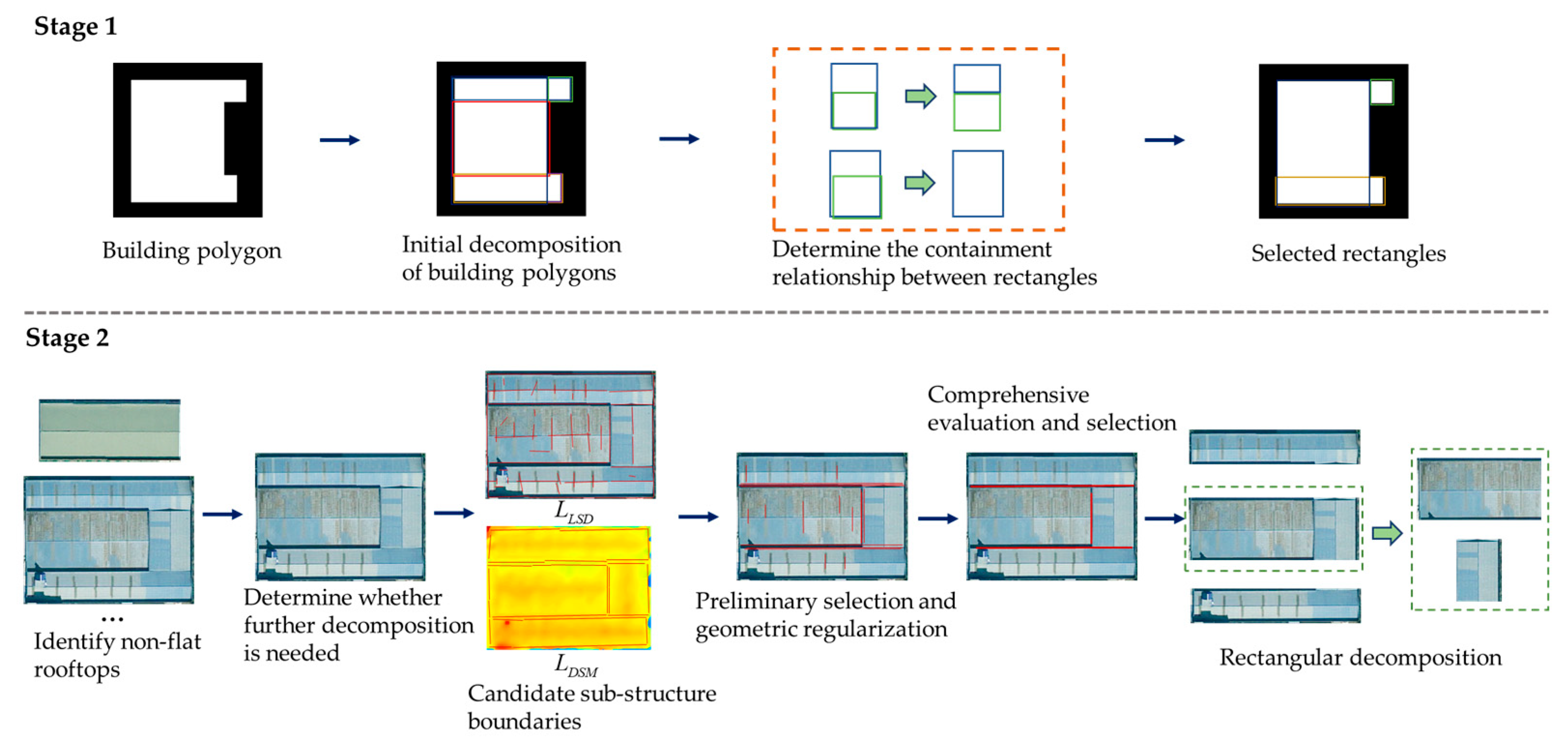
This study proposes an automated 3D building reconstruction method based on two-stage polygon decomposition and adaptive roof fitting. This subsection is organized into four parts: building polygon extraction and standardization, two-stage polygon decomposition and selection, 3D building model fitting, and model merging. First, building polygons are extracted and standardized to regularize the outlines while preserving salient footprint geometry. Next, a two-stage polygon decomposition strategy is introduced. In the first stage, polygons are coarsely decomposed and candidate rectangles are screened. In the second stage, non-flat regions are refined to accommodate complex inter-building connections. During model fitting, distinct strategies are adopted for flat and non-flat buildings, enabling accurate reconstruction of flat roofs with auxiliary structures as well as representative non-flat roof types. Finally, rectangular primitives with intersections are normalized and optimally merged, yielding high-accuracy, standardized building models. The overall workflow of the proposed method is shown in Figure 1.

3.1. Building Polygon Extraction and Standardization

A DSM-based building-mask refinement strategy was adopted following [16,27]. The masks were purified and boundary confidence increased by applying an SVM classifier [28] to gradient features extracted from the corresponding panchromatic (PAN) image. On this basis, a contour standardization method informed by regular structures was introduced to enhance structural consistency and geometric expressiveness. Constrained by the distribution of orientation angles and geometric continuity, the procedure sequentially performs orientation regularization, reconstruction of anomalous edges, and merging of co-oriented segments with small offsets. These steps suppress minor boundary distortions, short-edge perturbations, and spurious structures, thereby improving geometric completeness and the reliability and stability of subsequent modeling.
(1) Initial polygon fitting. The contour point set 𝒞 = { p i } i = 1 N ( p i = ( x i , y i ) ) is obtained by boundary tracing. A geometric approximation strategy [29] is then applied to derive a simplified polygon 𝒞 ^ , which effectively compresses redundant edge points while preserving the dominant structural outline.
(2) Minor kink detection and structural smoothing. To suppress sharp local corners introduced by mask noise or fitting errors, three consecutive vertices p i 1 , p i , and p i + 1 are considered. Let θ i 1 be the orientation of edge p i 1 p i , θ i the orientation of edge p i p i + 1 , and ϕ i the angular deviation between the adjacent edges. τ f is the minor kink threshold. When ϕ i = θ i θ i 1 < τ f , the corner is regarded as a minor kink without geometric salience and is removed to achieve local structural smoothing. In our implementation, setting τ f = 10 ° effectively suppresses jagged artifacts while preserving genuine small polylines.
(3) Principal-direction estimation. Orientation angles are computed for all edges of the initial building polygon and accumulated into a histogram over [ 0 ° , 90 ° ] with a 10 ° bin size, where orthogonal directions are folded into the same bin. The total edge length in each bin is summed, and only bins exceeding a predefined length threshold are retained. The principal-direction set 𝒟 = θ k is then obtained by taking the length-weighted mean orientation of each retained bin.
(4) Contour regularization by orientation. For each line segment p i p i + 1 formed by polygon vertices, its orientation angle φ i is computed.
φ i = arctan 2 ( y i + 1 y i , x i + 1 x i ) 180 π
Proximity to the principal-direction set 𝒟 = θ k is assessed by the absolute deviation between each edge’s orientation angle and the principal directions. τ θ is the tolerance threshold. If min θ k φ i θ k < τ θ , the segment is regularized by aligning it to the nearest principal direction. After alignment, intersections of adjacent edges are recomputed to update the vertices, and closure consistency as well as self-intersection repairs are performed to ensure geometric and topological validity. Segments without a matching direction are retained as free edges to minimize distortion. In our implementation, setting τ θ = 10 ° balances alignment success against false snapping.
(5) Short-edge regularization. Edges whose Euclidean length falls below a preset threshold are treated as spurious or perturbation edges. L i is the Euclidean length of the segment defined by vertices p i and p i + 1 , and τ s is the short-edge threshold. If L i = p i + 1 p i 2 < τ s , the edge is snapped to the nearest principal direction (or to a neighboring edge with a similar orientation), and its endpoints are reconstructed accordingly. In our implementation, setting τ s = 5   pix is recommended, as it substantially reduces noise without compromising the primary footprint.
(6) Merging co-oriented segments with small offsets. For two co-oriented line segments p i 1 p i and p i p i + 1 , the perpendicular offset between them is evaluated. Let Δ   denote the perpendicular offset and τ m the offset threshold. If Δ   = min ( x i + 1 x i , y i + 1 y i ) < τ m   , the segments are regarded as approximately collinear and are merged by snapping them to a common support line and reconstructing their endpoints. This operation enhances the overall coherence of the contour boundary and avoids redundant representations of repeated structures. In our implementation, setting τ m = 5   pix is recommended, as it effectively merges “ghost” parallel edges without collapsing genuine parallel walls.
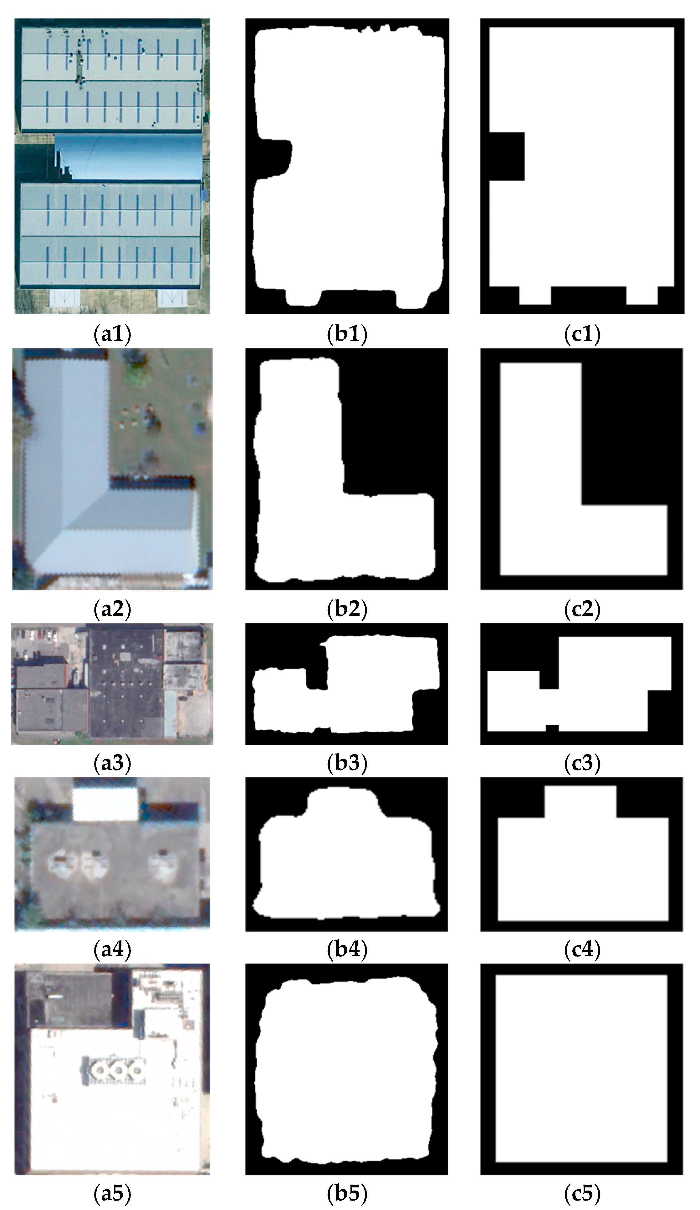
Figure 2 illustrates the standardization process for building polygons.
To further align the outlines with true object boundaries, image line segments are extracted from the orthophoto using the Line Segment Detector (LSD), and their orientation cues are used to locally correct edge directions [11]. Because most building polygons can be decomposed into rectangular primitives, the extracted polygons are rotated according to the first principal direction so that their dominant edges become approximately horizontal or vertical, thereby simplifying and improving the effectiveness of the subsequent polygon decomposition.

3.2. Two-Stage Polygon Decomposition and Selection

Given the limited set of primitive types available for fitting, the initial, morphologically complex building polygons must first be structurally decomposed and mapped to a set of parameterizable standard primitives to enable robust fitting and model integration. In this study, rectangular primitives are prioritized for decomposing the initial polygons. Because the decomposition proceeds primarily along the outer building boundary, a small number of non-rectangular primitives may also be introduced for complex outlines to ensure complete structural coverage. A two-stage polygon decomposition and selection method that fuses orthophotos and DSMs is proposed. Under a contour-fidelity constraint, the approach achieves comprehensive decomposition of complex building polygons, providing stable geometric support for subsequent 3D fitting and model merging.
After contour standardization and rotation, the first stage performs polygon decomposition and primitive screening with the goal of partitioning the footprint into basic rectangular units while preserving the outline. Concretely, for each edge on the outer boundary, an inward normal sweep is advanced within the building mask at a pixel step. If a counterpart parallel edge exists, the sweep terminates when the front enters the buffer zone defined by that parallel edge, and a candidate rectangle is generated. If no counterpart parallel edge exists, the sweep terminates when the advancing front is about to exit the mask, and a candidate rectangle is generated accordingly.
Using the boundary-segment inward sweep described above, a set of basic rectangular candidates is first produced. These candidates are then validated by removing any rectangle whose intersection-over-union with the building mask falls below a preset threshold T int . Setting T i n t = 0.9 enforces high conformity to the building polygon while retaining true rectangles with slight misalignment and avoiding shape bias. Potential containment relations among rectangles are also handled. Specifically, when a smaller rectangle is fully nested within a larger one, buffer bands are placed on both sides of their inclusion boundary (the internal contour formed by the intersection of the two rectangles). For an inclusion boundary L , buffer regions of width w are defined on its left and right, denoted B L 2 and B R 2 , respectively. Setting w = 5 pix enables effective comparison across the inclusion boundary. Discrimination across the inclusion boundary is performed using elevation, color, and local structural-gradient cues.
(1) Let the DSM elevation map be Z ( x , y ) . The mean elevations in the left and right buffer zones are
μ Z L   = 1 B L p B L Z ( p ) , μ Z R   = 1 B R p B R Z ( p )
The elevation-difference score is computed as
S z = μ Z L   μ Z R
(2) Let I ( p ) = [ R ( p ) , G ( p ) , B ( p ) ] T [ 0 , 255 ] 3 denote the orthophoto (intensity/color). The mean colors in the left and right buffers are
μ C L   = 1 B L p B L I ( p ) , μ C R   = 1 B R p B R I ( p )
The color-difference score is computed as
S c = μ C L   μ C R 2 T c
where T c is the color-difference threshold and S c is the normalized color-difference score. Considering transitions across roofs and materials, we set T c = 20 for 8-bit imagery.
(3) Let Z ( p ) denote the physically normalized DSM gradient at pixel p . The average gradient vectors in the left and right buffers are
μ G L   = 1 B L p B L Z ( p ) , μ G R   = 1 B R p B R Z ( p )
The gradient-difference score is computed as
S g = μ G L   μ G R
A composite score is formed as
S t o t a l = w z S z + w c S c + w g S g
In the composite score, the three terms S z , S c , and S g quantify elevation, color, and gradient differences, respectively, and the weights satisfy w z + w c + w g = 1 . The gradient term is more sensitive to boundary structures such as eaves, the color term is susceptible to illumination and material variations, and the elevation term complements geometric layering and step discontinuities. Accordingly, the composite score integrates elevation, color, and gradient cues to determine whether boundary structures are present. The weights w z = 0.3, w c = 0.2, and w g = 0.5 are determined by grid search and sensitivity analysis. If S t o t a l 0.5 , the small rectangle is retained as an independent structural unit.
In some inclusion boundaries, the left and right buffers exhibit nearly equal mean elevations, minor color variation, and gradients with opposite directions but similar magnitudes. Decisions may misclassify such cases. To improve robustness, a one-dimensional linear trend is fitted to all pixels in the left and right buffers B L and B R along the direction perpendicular to the inclusion boundary. Let the resulting ordered samples be ( x i , z i ) and ( x j , z j ) . We fit
z i = a L x i + b L , z j = a R x j + b R
where a L and a R are the local elevation change rates (slopes) on the two sides.
The small rectangle is retained as an independent structural unit if the following condition is met and the elevations on both sides of the inclusion boundary exhibit an upward trend.
sign ( a L ) sign ( a R )   and   a L , a R > T s l o p e
where sign ( ) is the sign function and T s l o p e is a slope threshold (set to T s l o p e = 0.4 ). Otherwise, the small rectangle is treated as redundant and discarded, and only the larger rectangle is kept as the primary structural region.
If the small rectangle is retained, the residual part of the large rectangle is further partitioned into new subrectangles to maintain full coverage. These newly generated subrectangles are screened using the same validity criteria to ensure that all retained units have clear structural significance.
After screening and retaining basic rectangles, any residual areas in the original building polygon that exceed a preset area threshold and cannot be effectively partitioned by the existing rectangular rules are preserved as non-rectangular structural units. Such regions typically form closed polygons (e.g., triangles) and are subsequently optimized uniformly as flat types. This strategy preserves the completeness of the building outline and improves geometric fidelity in complex scenes.
Following the first-stage coarse decomposition into basic rectangles, it was observed that rectangles generated solely by iterative boundary sweeps often fail to capture the true minimal building primitives (e.g., flat, hip, gable, pyramid, mansard). Even within a first-stage rectangle, multiple roof types may coexist. A second-stage rectangular refinement is therefore introduced. The framework for this stage is as follows:
(1) The rectangular region is first tested for a flat-roof composition. If the region is flat, no further subdivision is required; otherwise, a second-stage refinement is performed. An initial screening is conducted by checking whether the DSM elevation range within the rectangle is below a preset threshold T h = 1.0   m . If the flat criterion is not met, the interior structure is further analyzed based on normal-vector consistency. Local planes are fitted on the DSM using a 5 × 5 window to estimate a normal vector n ( x , y ) for each pixel. The rectangle is partitioned into an 8 × 8 grid, and within each cell the directional standard deviation σ n ( i ) of all normals is computed. Cells whose σ n ( i ) exceeds a threshold T n are flagged as exhibiting directional fluctuations, indicating potential non-flat roof features. Setting T n = 10 ° triggers detection of non-flat structures without oversensitivity. In parallel, DSM spatial gradients are used to detect pronounced slope changes. Sobel operators are applied to obtain the x- and y-direction gradient components, from which the gradient-magnitude image G ( p ) is computed. A high-gradient mask is then generated using a slope threshold T s l o p e = 0.4 . Connected components are extracted from this mask, and if any component exceeds a minimum area, the rectangular region is deemed to contain non-flat roof structures.
(2) To avoid unnecessary subdivision of rectangles that already exhibit clear structure, thereby preventing redundancy or distortion of the original geometry, a unimodality-based criterion is introduced. For each non-flat rectangle, the DSM is projected and averaged along the horizontal and vertical directions to produce two one-dimensional elevation profiles. To suppress noise, each profile is Gaussian-smoothed, after which peak detection [30,31] (combining peak salience and a minimum inter-peak distance) is applied to count the number of peaks, denoted N h and N v . Define
N p e a k s = max ( N h , N v )
Next, normalize the horizontal and vertical profile abscissae to [0,1]. Let t h and t v be the locations of the principal peaks on the two profiles. Define the minimum central deviation
Δ = min ( t h 0.5 , t v 0.5 )
The center offset threshold ε c detects whether the dominant peak of a one-dimensional profile is off center to trigger secondary subdivision. If N p e a k s > 1 , multiple undulations are present, suggesting multi-component assembly or juxtaposed slopes, and stage-two subdivision is triggered. If N p e a k s = 1 and Δ ε c ( ε c = 0.15 ), the region is considered a single slope and no subdivision is performed. If N p e a k s = 1 and Δ > ε c , the principal peak is markedly off-center, indicating a high likelihood of a “non-flat attached to flat” configuration, and stage-two subdivision is triggered. By exploiting distributional shape and geometric symmetry, the proposed strategy discriminates single from mixed components with greater robustness than methods that rely solely on amplitude-based indicators such as variance, gradient energy, or edge counts.
(3) For rectangles that satisfy the subdivision criteria, finer substructures are extracted by fusing orthophoto and DSM cues. Significant line segments are first detected on the orthophoto using the Line Segment Detector (LSD) to form a set L LSD . In parallel, a gradient-magnitude map G ( x , y ) is computed from the DSM. High-structure-change regions are obtained by thresholding G ( x , y ) with T s l o p e = 0.4 and enhancing connectivity via morphological erosion-dilation. Approximate straight segments are then extracted from these connected high-gradient regions using the Hough transform to form a set L DSM .
Candidate segments are filtered and regularized as follows: (i) remove segments within 5 pix of the building boundary; (ii) discard segments shorter than 5 pix; (iii) reject segments whose orientation deviates from horizontal or vertical by more than 10 ° ; (iv) merge adjacent short segments whose mutual angle is below 10 ° and refit them with least squares to obtain a single line; (v) snap near-axis segments to the canonical directions by setting the orientation θ = 0 ° if θ < 10 ° and θ = 90 ° if θ 90 ° < 10 ° . To avoid misclassification due to ridgelines and other internal roof structures, the elevation trend on both sides of each candidate line is analyzed in narrow buffers. If elevations on both sides decrease monotonically away from the line, the segment is labeled as an internal roof structure and removed. Finally, the surviving segments are merged to yield the candidate set of substructure demarcation lines L = L LSD L DSM .
For each candidate substructure boundary, buffer zones are constructed on its left and right sides. A combined decision is then made using elevation differences, color changes, and gradient variations across the buffers to discard boundaries that fail the criteria. When two co-directional boundaries are closer than 5 pix, a special-case test is first applied (see Equation (10)). If no special case is detected, a composite score is computed (see Equation (8)), and the boundary with the higher score is retained.
The selected boundaries are horizontal or vertical, yielding three decomposition cases for the rectangular region: (1) only horizontal boundaries are present, so the region is split along the horizontal direction; (2) only vertical boundaries are present, so the region is split along the vertical direction; (3) both horizontal and vertical boundaries are present. To robustly handle case (3), the ratio of each horizontal boundary’s length to the rectangle’s horizontal edge length is computed and averaged; the same is done for vertical boundaries relative to the vertical edge length. The direction with the higher average coverage ratio (horizontal or vertical) is selected for the initial split. After partitioning the region into subrectangles, a second split is performed along the orthogonal direction to achieve complete decomposition. Figure 3 illustrates the two-stage building polygon decomposition and selection process.
In summary, a two-stage polygon decomposition method that fuses orthophoto and DSM information is proposed. The approach improves the completeness and semantic consistency of complex building structures and is suitable for multi-level building analysis aimed at structured modeling.

3.3. 3D Model Fitting

We noted in the previous subsection that only non-flat rectangles undergo second-stage subdivision. Accordingly, 3D model fitting is performed separately for flat rectangles, non-flat rectangles, and non-rectangular regions. Non-rectangular regions are optimized under the assumption of a fully flat roof. For flat rectangles, we first test whether the rooftop shows appreciable elevation variation. If it does, adaptive rooftop partitioning driven by the DSM elevation distribution is applied to refine heights; otherwise, the roof is modeled as perfectly flat. For non-flat rectangles, which have already been fully subdivided, parameter analysis and 3D optimization are conducted for common roof types (gable, hip, pyramid, mansard). The 3D model-fitting procedures for flat and non-flat rectangular regions are described in detail below.
(1) 3D model optimization of flat rectangular buildings via DSM-based regional structure analysis and adaptive rooftop partitioning. Given the elevation values D ( x , y ) within the rectangle and the footprint parameters L, W obtained from the fitted polygon, the rectangle’s elevations are discretized into a finite set of bins.
bin k = [ h k δ , h k + δ ] , k = 1 , 2 , , K
where the elevation tolerance δ is adaptively estimated from the histogram’s peak distribution, and the number of elevation partitions K is automatically determined by the number of significant peaks in the histogram.
For each bin, a binary mask M k ( x , y ) is generated. Connected components are extracted from M k ( x , y ) to obtain salient regions. Region filtering is then applied to suppress noise, followed by morphological erosion-dilation to remove boundary artifacts and restore the main shapes, improving segmentation stability.
The boundary points of each connected region are extracted as B i = { ( x j , y j ) } , and all boundary points are merged to form B = i = 1 N B i . These points are projected onto the rectangle’s horizontal and vertical axes to obtain two one-dimensional point sets.
P x = { x j | ( x j , y j ) B } ,   P y = { y j | ( x j , y j ) B }
One-dimensional density estimation is performed separately on P x and P y to analyze the distribution of boundary points and to identify cluster centers or change points that indicate cut locations in the two directions. Projected points closer than 5% of the building size are merged, and points within 5% of the outer boundary are discarded. This yields the horizontal and vertical cut sets 𝒞 x and 𝒞 y , respectively.
The rectangle is then partitioned by 𝒞 x and 𝒞 y into subrectangular units R m , n , where m and n index the horizontal and vertical cuts. The geometric parameters of a flat rectangular building are defined as
Ψ = { C , H , P }
where C = { L , W } contains the footprint parameters, H = { h m , n | m = 1 , 2 , , M , n = 1 , 2 , , N } is the heights of the subrectangles, and P = { x 1 , x 2 , , x M 1 , y 1 , y 2 , , y N 1 } specifies the horizontal and vertical cut positions.
An initial set of subrectangles is constructed from the predetermined horizontal and vertical cut positions, and each subrectangle is assigned an initial height equal to its mean value h ¯ m , n . To further improve geometric accuracy and structural plausibility, a global parameter search is formulated using the Artificial Bee Colony (ABC) algorithm [32,33,34,35]. The colony size is set to 20, the maximum cycle number to 10,000, and the abandonment limit to 30. These parameter values were determined through preliminary experiments to balance reconstruction accuracy and computational efficiency, with their robustness confirmed across multiple datasets and scenarios. In this framework, each bee encodes a complete model configuration that includes the subrectangle boundary positions and their associated heights. During optimization, local exploration by employed bees and information sharing with onlooker bees drive iterative updates of the model parameters. Because cuts follow axis-aligned boundaries, the partition remains complete and free of overlaps or discontinuities. The fitness function therefore focuses on two aspects: the height error of each subregion relative to the DSM and the height coherence between adjacent subrectangles. Height coherence encourages neighboring units with similar initial elevations to converge to a common height, which preserves roof continuity and smoothness and reduces local artifacts. To enhance global convergence and maintain diversity, the perturbation radius and population distribution strategy are adapted dynamically during the search. The converged parameters are then used to construct a regularized flat rectangular 3D model, improving geometric accuracy and semantic consistency. The ranges for the optimized parameters h m , n , x m , and y n are set to h m , n [ h ¯ m , n 3 , h ¯ m , n + 3 ] , x m [ x j 1 / 8   L , x j + 1 / 8   L ] , and y n [ y j 1 / 8   W , y j + 1 / 8   W ] , respectively.
(2) 3D optimization of non-flat rectangular buildings based on roof-type analysis. For non-flat rectangular regions, together with DSM/nDSM cues, roofs can be fitted using simple parametric models. Four roof types are considered: gable, hip, pyramid, and mansard (Figure 4), each described by a small set of geometric parameters. Following the parameterization in [11,14], the geometry is defined as
Φ = { P , C , S }
where P = { x o , y o , o r i e n t a t i o n } contains the location parameters, C = { L , W } is the contour parameters, and S = { Z r i d g e , Z e a v e , h i p l , h i p w } contains the shape parameters.
For each of the four non-flat roof types, geometric parameters are initialized as follows:
Gable: longitudinal hip distance h i p l ( 0 ) = 0 ; latitudinal hip distance h i p w ( 0 ) = W / 2 ; ridge height Z r i d g e ( 0 ) = H ¯ ; eave height Z e a v e ( 0 ) = H ¯ 0.5   m . H ¯ is calculated as the mean elevation based on the building polygon.
Hip: longitudinal hip distance h i p l ( 0 ) = L / 4 ; latitudinal hip distance h i p w ( 0 ) = W / 2 ; ridge height Z r i d g e ( 0 ) = H ¯ ; eave height Z e a v e ( 0 ) = H ¯ 0.5   m .
Pyramid: longitudinal hip distance h i p l ( 0 ) = L / 2 ; latitudinal hip distance h i p w ( 0 ) = W / 2 ; ridge height Z r i d g e ( 0 ) = H ¯ ; eave height Z e a v e ( 0 ) = H ¯ 0.5   m .
Mansard: longitudinal hip distance h i p l ( 0 ) = L / 4 ; latitudinal hip distance h i p w ( 0 ) = W / 4 ; ridge height Z r i d g e ( 0 ) = H ¯ ; eave height Z e a v e ( 0 ) = H ¯ 0.5   m .
Given these initializations, an exhaustive search on S = { Z r i d g e , Z e a v e , h i p l , h i p w } is performed using the DSM to identify the model and parameter set that minimize RMSE. To balance accuracy and computational cost, discrete step sizes are applied to the parameter grid. The ranges and step sizes for all parameters are listed in Table 1.

3.4. 3D Model Merging

A building’s 3D model comprises multiple primitives that may intersect. During polygon decomposition, inclusion relations between rectangular primitives were considered, allowing L-shaped and T-shaped buildings to be distinguished as adjacent or intersecting. Here, we focus on merging primitives that intersect. Because primitives are fitted independently, DSM quality can affect both optimization outcomes and roof-type classification. We first normalize the types of intersecting primitives using a roof-type decision matrix so that intersecting units are treated as rectangles of the same roof class [11]. Then, the 3D building model merging method proposed in [16] is applied. Since the mansard model is the most parameterized roof type, it can be specialized to other roofs with fewer parameters. Optimization and merging are performed according to the roof type of the intersecting primitives.

4. Experimental Results

This section presents qualitative and quantitative experiments to evaluate the proposed automated 3D building reconstruction method. The experiments cover the datasets and evaluation metrics, parameter settings, parameter analysis, results of polygon standardization, analysis of polygon decomposition, and comparisons with representative state-of-the-art methods.

4.1. Experimental Data and Evaluation Metrics

This study uses three datasets: (1) Beijing-3, (2) SuperView-1, and (3) US3D.
Beijing-3 [36] covers an urban area of Beijing, with imagery acquired on 3 December 2021. The dataset comprises 0.3 m panchromatic (PAN) imagery, 1.2 m multispectral (MS) imagery, pansharpened RGB at 0.3 m, and stereo satellite-derived DSMs at 0.3 m. Ground-truth DSMs were produced by UAV-based oblique photogrammetry.
SuperView-1 [37] covers a campus area in Harbin, Heilongjiang, acquired on 4 May 2020. It includes 0.5 m PAN, 2 m MS, pansharpened RGB at 0.5 m, and stereo satellite-derived DSMs at 0.5 m. Ground-truth DSMs were obtained from airborne LiDAR.
US3D [38] contains 26 WorldView-3 images over Jacksonville (JAX), Florida (2014–2016), and 43 WorldView-3 images over Omaha (OMA), Nebraska (2014–2015). WorldView-3 provides 0.31 m PAN and 1.24 m MS imagery; the dataset includes pansharpened RGB at 0.31 m and stereo satellite-derived DSMs at 0.31 m. Ground-truth DSMs were obtained from airborne LiDAR.
Initial building reconstructions were generated using a stereo matching method based on iterative optimization of hierarchical graph structure consistency cost [39].
This study employs the following evaluation metrics [11,15,16,40,41] to assess the quality of the reconstructed 3D building models.
(1) Root mean square error (RMSE): the standard deviation of the residuals between the ground truth and the predicted DSM.
R M S E = 1 N i = 1 N ( h i h ^ i ) 2
where N denotes the number of test pixels, and h i and h ^ i denote ground-truth and predicted heights, respectively.
(2) Median height error (MHE): the median value of the absolute error between the ground truth and the predicted DSM.
M H E = m e d i a n i [ 1 , N ] ( h i h ^ i )
(3) 2D Intersection over Union (IOU2) evaluates the overlap between the reconstructed and reference building footprints.
I O U 2 = T P T P + F P + F N ,
where TP is the number of pixels predicted as building and labeled as building, FP is predicted building but labeled non-building, and FN is predicted non-building but labeled building.
(4) 3D Intersection over Union (IOU3) measures the overlap between the reconstructed and reference 3D building models.

4.2. Experimental Parameter Setting

We provide detailed settings for the key parameters used in the automated 3D building reconstruction pipeline. In polygon extraction and standardization, the thresholds are set to τ f = 10 ° , τ θ = 10 ° , τ s = 5   pix , τ m = 5   pix . In the two-stage polygon decomposition and selection, Stage 1 uses an IOU selection threshold T i n t = 0.9 , a buffer width w = 5   pix , a color-difference threshold T c = 20 , a slope threshold T s l o p e = 0.4 , and weighting coefficients w z = 0.3, w c = 0.2, and w g = 0.5. Stage 2 employs a height threshold T h = 1.0   m , a directional fluctuation threshold T n = 10 ° , and a center offset threshold ε c = 0.15 . During 3D model fitting, flat rectangular regions are optimized with an Artificial Bee Colony algorithm over the ranges h m , n [ h ¯ m , n 3 , h ¯ m , n + 3 ] , x m [ x j 1 / 8   L , x j + 1 / 8   L ] , and y n [ y j 1 / 8   W , y j + 1 / 8   W ] . Non-flat rectangular regions are optimized by exhaustive search over Z e a v e [ Z e a v e ( 0 ) 3 , Z e a v e ( 0 ) + 3 ] , Z r i d g e [ Z e a v e + 0.5 , Z e a v e + 4 ] , h i p l [ h i p l ( 0 ) 1 / 8   L , h i p l ( 0 ) + 1 / 8   L ] , and h i p w [ h i p w ( 0 ) 1 / 8   W , h i p w ( 0 ) + 1 / 8   W ] .
In this paper, most parameters (e.g., T h , T s l o p e , τ θ , τ f , w z , w c , w g ) are insensitive to image resolution and scene variation. Only the short-edge threshold τ s , the offset threshold τ m , and the buffer width w show mild dependence on resolution. Under our experimental conditions, setting τ s = 5   pix , τ m = 5   pix , and w = 5 pix corresponds to a physical scale of approximately 1.5 to 2.5 m, which lies within the performance plateau identified by our sensitivity analysis. Accordingly, a fixed parameter set is used throughout the experiments.

4.3. Experimental Parameter Analysis

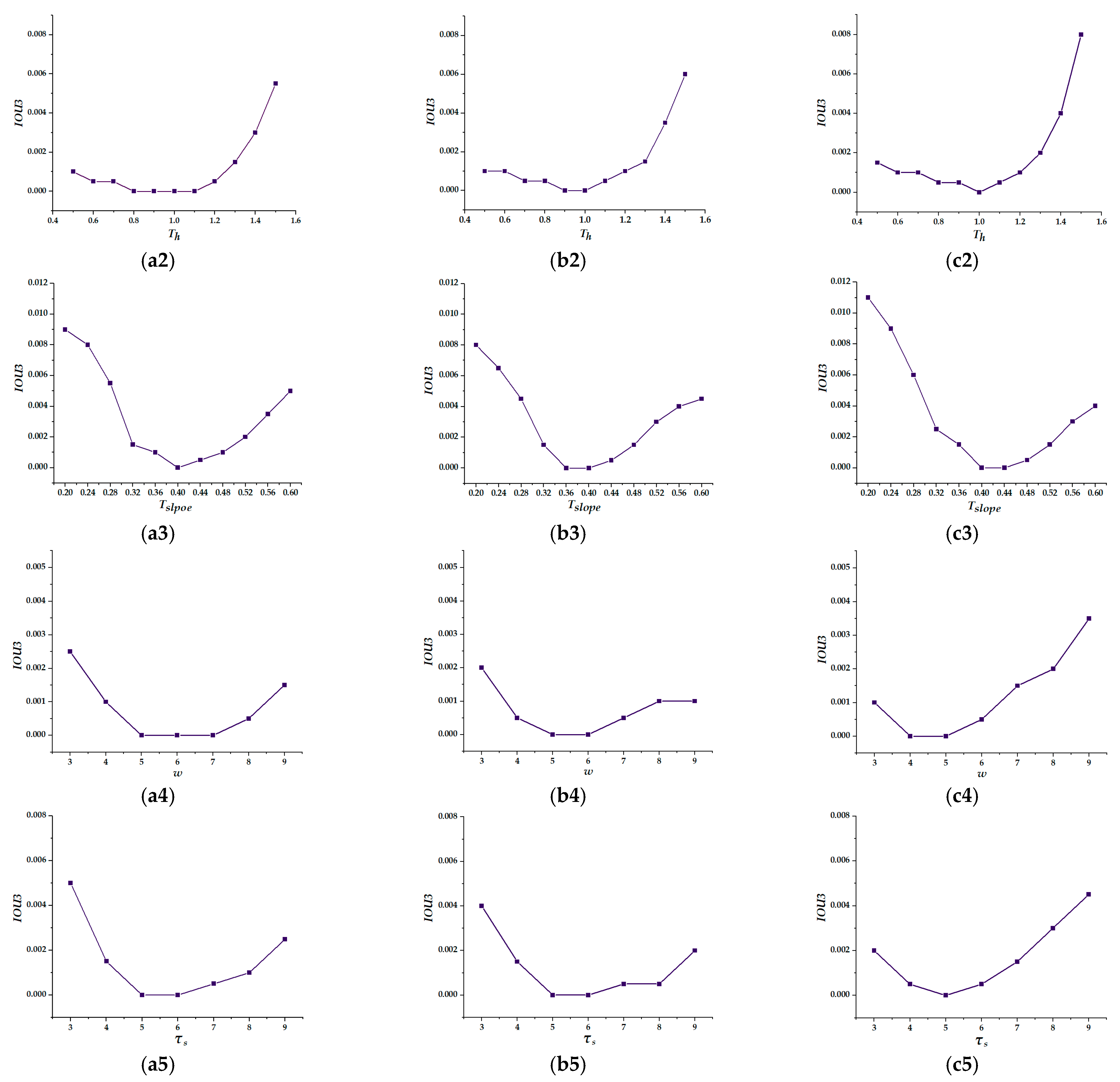
This section analyzes the influence of key experimental parameters on 3D building modeling, including the weighting coefficients w z , w c , and w g , a height threshold T h , a slope threshold T s l o p e , the buffer width w, and the short-edge threshold τ s . Figure 5 illustrates the impact of parameter settings on 3D building modeling across different datasets. Using the optimal configuration as a baseline (IOU3 = 0), changes in IOU3 are evaluated under alternative settings.
The weighting coefficients w z , w c , and w g jointly affect the first-stage polygon decomposition. A grid search was conducted with w g [ 0.1 , 0.8 ] , w c [ 0.1 , 0.8 ] , w z [ 0.1 , 0.8 ] (step 0.1) to analyze how different weight settings affect 3D building reconstruction. From Figure 5(a1–c1), when w c is fixed, increasing w g while decreasing w z yields an IOU3 curve that first declines and then rises; when w g is fixed, increasing w c while decreasing w z produces an overall increase; when w z is fixed, increasing w g while decreasing w c produces an overall decrease. These results indicate that the gradient term is dominant in the first-stage decomposition, whereas the color term is comparatively less influential. Across datasets, stable performance is achieved with w z = 0.3, w c = 0.2, and w g = 0.5.
The height threshold T h affects the second-stage polygon decomposition. If T h is set too low, minor elevation undulations are treated as structural signals, which triggers unnecessary subdivision and increases complexity. If T h is set too high, non-flat roofs may be misclassified as flat, leading to detail loss and degraded modeling. As shown in Figure 5(a2–c2), IOU3 typically exhibits a slight initial decrease followed by a rapid increase as T h grows. Owing to dataset characteristics, Beijing-3 performs best for T h [ 0.8 , 1.1 ] , US3D for T h [ 0.9 , 1.0 ] , and SuperView-1 at T h = 1.0 , suggesting low sensitivity to dataset differences. We therefore recommend T h = 1.0 .
The slope threshold T s l o p e is used to identify high-gradient regions. If T s l o p e is set too low, local noise and weak textures are amplified as “high-gradient” evidence, producing spurious cuts. If T s l o p e is set too high, true weak edges are missed, resulting in under-segmentation. As shown in Figure 5(a3–c3), IOU3 decreases rapidly at first and then increases as T s l o p e grows, with the decline steeper than the rise. This suggests that insufficient noise suppression harms modeling more than missing weak edges. Beijing-3 performs best at T s l o p e = 0.4 , US3D with T s l o p e [ 0.36 , 0.40 ] , and SuperView-1 with T s l o p e [ 0.40 , 0.44 ] , indicating limited sensitivity to dataset differences. We therefore recommend T s l o p e = 0.4 .
The buffer width w compares elevation, color, and gradient differences within buffers on both sides of the inclusion boundary of nested rectangles. If w is set too small, statistics are unstable. If w is set too large, cross-boundary sampling may occur. As shown in Figure 5(a4–c4), IOU3 first decreases and then increases as w grows. The decline is faster than the rise for Beijing-3 and US3D, while the opposite trend is observed for SuperView-1. Due to resolution differences, Beijing-3 performs best for w [ 5 , 7 ] , US3D for w [ 5 , 6 ] , and SuperView-1 for w [ 4 , 5 ] . Within 0.3 to 0.5 m resolution, w is not sensitive, and w = 5 pix is recommended.
The short-edge threshold τ s filters extremely short pseudo-edges during building polygon extraction. If τ s is set too small, spurious short edges remain. If τ s is set too large, true short edges are removed and roof details are lost. As shown in Figure 5(a5–c5), IOU3 first decreases and then increases as τ s grows. The decrease is faster than the increase for Beijing-3 and US3D, while the opposite holds for SuperView-1. Due to resolution differences, Beijing-3 performs best for τ s [ 5 , 6 ] , US3D for τ s [ 5 , 6 ] , and SuperView-1 at τ s = 5 . This suggests that τ s is not sensitive within 0.3 to 0.5 m resolution. We therefore recommend τ s = 5 pix.

4.4. Standardization Results of Building Polygons

Standardizing building polygons is a critical step in 3D building reconstruction. A contour regularization method informed by structural regularity is adopted to normalize building polygons, thereby enhancing structural consistency and geometric expressiveness and establishing a solid basis for subsequent polygon decomposition. Figure 6 illustrates standardized results for buildings of diverse shapes, including the original satellite imagery, building masks derived from the DSM, and the standardized building outlines obtained after polygon regularization. As shown, masks extracted directly from the DSM exhibit notable boundary deficiencies. On the one hand, due to the DSM’s finite resolution and interference from surrounding objects, the raw outlines commonly appear jagged with coarse edges, and some regions contain small spurious structures or discontinuous boundary perturbations. On the other hand, the raw masks often fail to capture the global geometric characteristics of buildings, introducing significant redundancy for subsequent modeling and geometric representation.
After applying the proposed polygon standardization, the outer building contours are substantially improved. Specifically, the regularized outlines preserve the principal building shape while effectively removing spurious boundary segments, eliminating insignificant local kinks and short edges, and enforcing directional constraints to align with the dominant structural orientations. This process not only reduces the number of redundant vertices, yielding a more compact and concise representation, but also strengthens structural integrity and geometric regularity. The resulting standardized polygons are thus cleaner and more uniform, accurately delineating the primary building morphology and providing more reliable inputs for downstream polygon decomposition, parameter extraction, and 3D model fitting.

4.5. Analysis of Building Polygon Decomposition

In general, automated 3D building reconstruction comprises multiple components and entails a complex workflow. This section focuses on the building polygon decomposition stage and compares the proposed two-stage polygon decomposition and selection method with several existing approaches.
The compared polygon decomposition methods include that of Partovi et al. [16], who introduced a parallel-line-based decomposition technique. Their method iteratively translates line segments until they intersect with the buffer zone of another parallel segment and then forms rectangles from the resulting line pairs. Gui et al. [11] proposed a grid-based rectangle decomposition method that converts complex building polygons into a set of fundamental rectangular units to support subsequent model fitting.
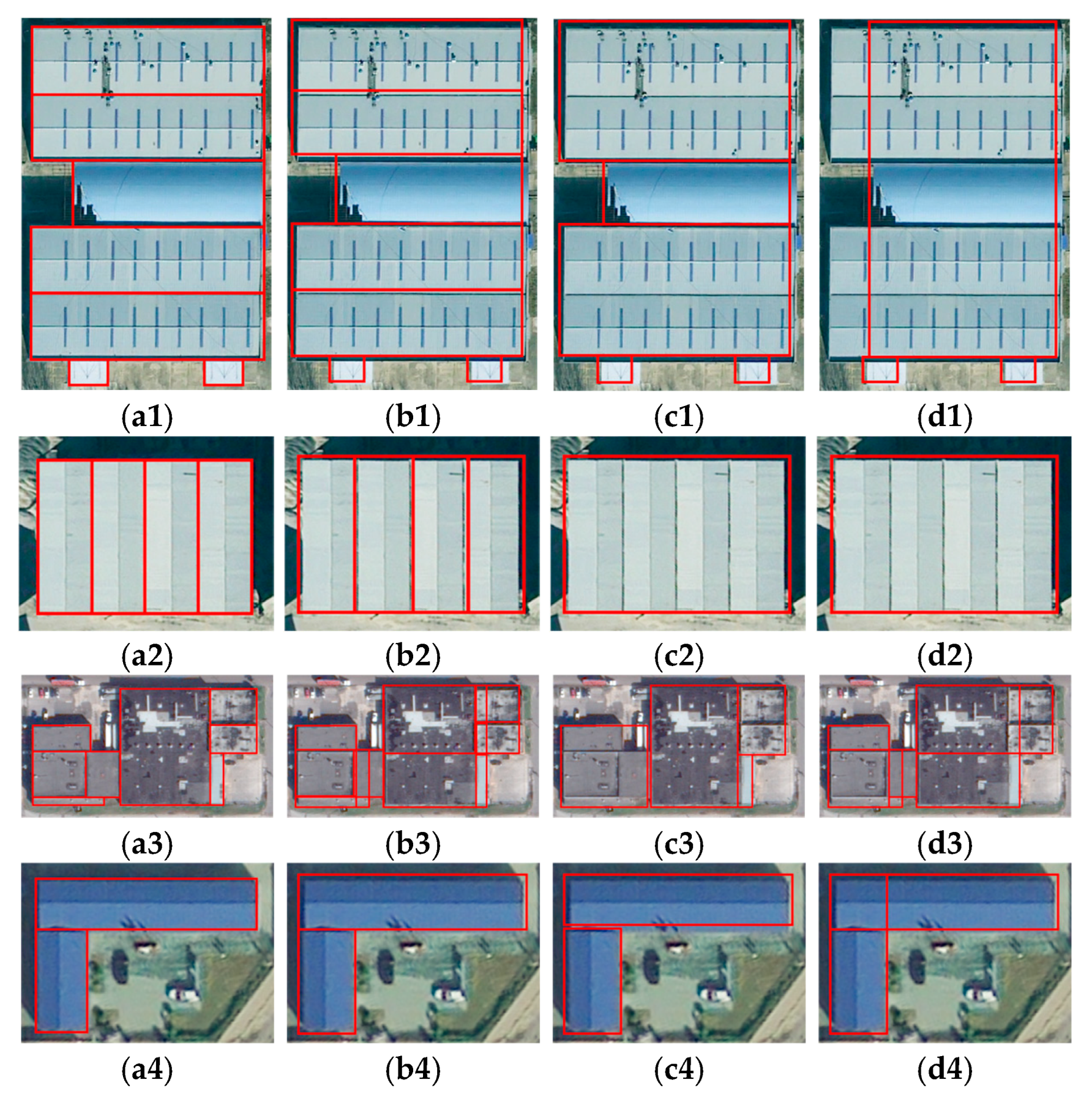
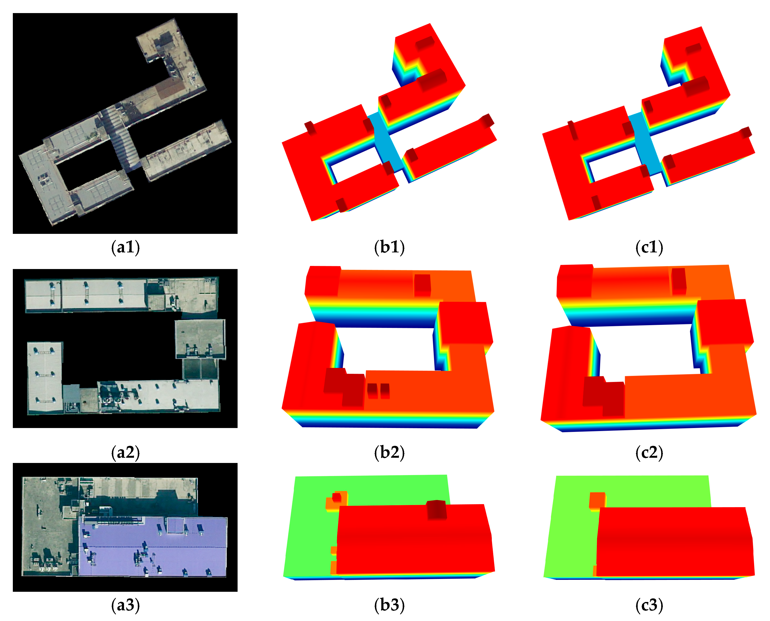
To ensure a fair evaluation of building polygon decomposition, the same polygonal inputs described in Section 3.1 were used. Figure 7 presents the visual results of building polygon decomposition for all methods, while Table 2 summarizes their quantitative evaluation. Two metrics, IOU2 and IOU3, were employed to assess decomposition accuracy at the 2D and 3D levels, respectively. As shown in the figure, different decomposition strategies yield markedly distinct outcomes, which further propagate to the 3D modeling stage. Although the IOU2 metric exhibits limited discriminative power, the IOU3 metric reveals more substantial performance differences. From the visual comparison of building polygon decomposition, Partovi et al.’s approach does not fully consider complex substructures and mainly relies on overlap ratios for selection, leading to incomplete coverage and insufficient decomposition of composite forms, thereby reducing 3D model accuracy. Gui et al.’s method shows limited capability in separating adjacent building structures with similar appearance, often failing to achieve accurate polygon partitioning and thus compromising reconstruction precision. In contrast, the proposed two-stage polygon decomposition approach achieves more accurate polygon partitioning, preserves the overall structural morphology, and produces 3D building models with higher geometric fidelity.

4.6. Comparison to State-of-the-Art Methods

To comprehensively evaluate the proposed automated 3D building reconstruction method, several representative baselines were selected for comparison: ALOD2MR [11], ABMR [16], PLANES4LOD2 [15], SAT2LOD2 [18], RDISCMR [8], and FusedSeg-HE [42]. All baseline methods in the comparative experiments were configured strictly according to the parameter settings recommended in their original papers, as specifically follows:
ALOD2MR: The empirical threshold, minimum edge length threshold (in pixels), adjacency distance threshold (in pixels), height difference threshold (in meters), and height gradient threshold (in meters) were set to T w , T l , T d , T h 1 , T h 2 = 0.2 , 120 , 10 , 1 , 0.2 .
ABMR: The roof center offset parameter was optimized with a step size of 1 pixel; the eave height and ridge height parameters were searched with a step size of 0.2 m; and the roof length and roof width parameters were updated using a step size of 1 m.
PLANES4LOD2: The cross-entropy class weights were set as follows: background, 1.0; roof plane separation, 6.0; building section separation, 6.2; and building segment, 1.5. The topological loss weights were set to 0.05 for building segments and 0.10 for separation lines.
SAT2LOD2: The minimum edge length threshold (in pixels), adjacency distance threshold (in pixels), height difference threshold (in meters), and height gradient threshold (in meters) were set to T l , T d , T h 1 , T h 2 = 90 , 10 , 0.5 , 0.1 .
RDISCMR: Each vertex was allowed to move among 42 predefined candidate positions in 3D space. The consistency constraint loss between corresponding left-right epipolar lines was assigned a weighting factor of 0.3.
FusedSeg-HE: The Adam optimizer was adopted with a learning rate of 5 × 10 5 , 70 training epochs, a batch size of 1, and a segmentation loss weight of λ = 0.005 .
ABMR and ALOD2MR are traditional pipelines comprising building polygon extraction, polygon decomposition, and 3D model fitting. PLANES4LOD2, RDISCMR, and FusedSeg-HE are deep learning-based approaches for 3D building reconstruction, while SAT2LOD2 (PC version with NVIDIA CUDA 11 support) is a software-driven solution. Figure 8 visualizes reconstructions from the proposed method and the baselines. Visually, our method produces models that are closer to the reference, recovering fine architectural details and correctly assigning roof types to rectangular subregions within each footprint. Among the traditional methods, ALOD2MR generally outperforms ABMR, yet both suffer from incomplete polygon decomposition, which leads to missing details and inadequate preservation of complex building outlines. Among deep learning-based methods, PLANES4LOD2 yields standardized 3D building models. RDISCMR optimizes vertex positions by learning point-cloud displacements, and FusedSeg-HE fuses convolutional and vision transformer encoders for object height estimation, but neither imposes standardization constraints. As a result, RDISCMR and FusedSeg-HE often exhibit elevation fluctuations over flat roofs and lack smoothly varying elevations over non-flat roofs. PLANES4LOD2 enforces standardization while better preserving the primary building structure, whereas RDISCMR and FusedSeg-HE, despite the absence of standardization, recover many local details. The software-based SAT2LOD2 tends to lose considerable fine-scale information.
Table 3 reports quantitative results on representative buildings. Three metrics are used: IOU3 to assess 3D volumetric accuracy, and RMSE and MHE to assess 2D elevation accuracy and stability. The results show that our method achieves the closest agreement with the reference in 3D (highest IOU3) and the best 2D elevation accuracy and stability (lowest RMSE and MHE). PLANES4LOD2 ranks second overall, followed by RDISCMR.
We further visualized the method’s outputs on more complex and diverse buildings (Figure 9). These buildings exhibit high structural complexity, highly irregular outlines, and dense mixtures of multiple building types. The visualizations indicate that the method effectively reconstructs buildings with intricate connectivity and preserves the primary outlines and geometry. Very small auxiliary elements may be attenuated or missed, yet the main structures remain complete and coherent. These results substantiate the effectiveness and robustness of the method in complex urban settings.
To demonstrate the robustness of the proposed method, experiments were conducted on 148 buildings. Table 4 reports averaged performance across 3D and 2D metrics for our approach and representative baselines. The proposed method achieved the best overall performance, with mean IOU3 of 91.26%, RMSE of 0.78 m, and MHE of 0.22 m. Among traditional methods, ALOD2MR outperformed ABMR, attaining 85.54% IOU3, 1.49 m RMSE, and 0.45 m MHE, compared with 83.17%, 1.71 m, and 0.54 m, respectively. Among deep learning-based methods, PLANES4LOD2 performed best (IOU3 88.36%, RMSE 1.35 m, MHE 0.32 m), followed by RDISCMR (86.32%, 1.37 m, 0.36 m) and FusedSeg-HE (85.89%, 1.41 m, 0.37 m). The software-based SAT2LOD2 yielded 83.68% IOU3, 1.60 m RMSE, and 0.51 m MHE. These qualitative and quantitative results indicate that the proposed method provides an effective and accurate solution for 3D building model reconstruction.

5. Discussion

5.1. Method Applicability Analysis

To further demonstrate the effectiveness of the proposed method, additional experiments were conducted in which the original datasets were degraded by (i) two-fold downsampling in resolution, (ii) additive Gaussian noise with σ = 10, and (iii) partial occlusions implemented as 7 × 7 patches on roof surfaces with pixel values set to zero. Fifty buildings were randomly selected from the datasets for evaluation.
Table 5 presents the performance of the proposed method on degraded data, with quantitative evaluations conducted for three typical degradations: resolution reduction, noise injection, and occlusion. Experimental results demonstrate that noise and small-area occlusion have minimal impact on 3D modeling quality at the specified degradation levels. Although resolution reduction exhibits a more pronounced effect on reconstruction quality, all evaluation metrics remain within acceptable ranges. Given that sub-meter or higher resolution satellite imagery is common in urban applications, resolution is typically not the primary bottleneck, whereas occlusions, disparity discontinuities, and local matching errors are more challenging. Overall, the results in Table 5 show that the proposed automated 3D building reconstruction method remains stable under noise, occlusion, and reduced-resolution conditions, demonstrating generalizability and robustness.

5.2. Computational Efficiency Analysis

Under the two-stage decomposition and adaptive roof fitting framework, the overall complexity is approximately proportional to the product of the number of buildings, the number of primitives per building, the number of roof candidates per primitive, and the number of parameters per roof type. In practice, both the number of primitives per building and the number of candidates per primitive are small, typically in the single digits. As a result, the overall complexity increases approximately linearly with the number of buildings, making the method suitable for scaling to large scenes. The “exhaustive search” employed here is a finite, constrained search over a few typical roof types with discretized parameters. Consequently, the search scale is controllable and computationally modest. In addition, the fitting process for individual buildings or tiles is mutually independent, making the algorithm inherently suitable for building-level or block-level parallelization. Taking accuracy and computational complexity into account, the overall efficiency of the proposed method is acceptable and competitive in practical engineering applications.

5.3. Applicability, Limitations, and Future Work

This study targets 3D building model reconstruction from satellite imagery. The method is centered on rectangular primitives and is designed to efficiently reconstruct regular buildings that can be covered by a finite set of rectangular subregions. Such structures are common in urban scenes, where plan outlines are approximately orthogonal or can be adequately represented with a small number of rectangular decompositions. The proposed two-stage polygon decomposition with adaptive roof fitting reconstructs standardized 3D models while preserving building boundaries as much as possible. The method is most suitable for rectangular buildings or for buildings that can be decomposed into multiple rectangles, including cases with complex connections and flat roofs with auxiliary structures. In the first stage, most rectangles are fitted to the original building polygon to retain outline detail. If significant non-rectangular residual regions remain, for example, triangular parts, they are conservatively modeled under a flat roof assumption to preserve the true boundary shape.
The approach has limitations in several scenarios. (1) Streamlined or highly irregular buildings are approximated by piecewise straight segments in the current framework, which may lead to loss of curvature. (2) For non-rectangular building regions, boundary preservation is prioritized and residual areas are modeled under a flat-roof assumption, which can introduce local elevation bias. (3) For non-flat roofs with complex auxiliary structures, the method addresses only common non-flat types and does not explicitly model additional attachments, which limits reconstruction fidelity in such cases. Future work will expand the primitive set and introduce deformable rectangles and spline-based outlines to better accommodate streamlined and highly irregular targets.

6. Conclusions

This paper presents an automated 3D building reconstruction method based on two-stage polygon decomposition and adaptive model fitting. First, building polygons are extracted and standardized to preserve the principal outline while enhancing geometric expressiveness. On this basis, a two-stage polygon decomposition strategy is designed: in Stage 1, polygons are coarsely partitioned and rectangular primitives are screened using inclusion relations, and in Stage 2, regions with complex connections are fully decomposed to obtain finer structural representations. Differentiated modeling strategies are then applied: for flat roofs, DSM-based regional structure analysis and adaptive top-surface partitioning enable accurate modeling of targets with auxiliary components, and for non-flat roofs, systematic exploration and optimization are employed to select the optimal parameters across multiple roof types. Finally, intersecting rectangular primitives are normalized and optimally merged to improve model consistency and completeness. Experiments over diverse and numerous buildings demonstrate clear advantages for structures with complex roof patterns or tightly coupled components. Compared with representative baselines, the proposed method achieves the best overall performance, with mean IOU3 of 91.26%, RMSE of 0.78 m, and MHE of 0.22 m, confirming its effectiveness and superiority for automated 3D building reconstruction.
To meet the demands of city-scale reality modeling, future work will directly address the limitations identified in this study. Deformable rectangles and spline-based outlines will be introduced to reduce curvature loss caused by approximating streamlined or highly irregular buildings with straight segments, and the primitive library will be expanded to accommodate a broader range of building types. In parallel, texture-mapping techniques will be investigated on the reconstructed models to enhance realism and visualization.

Author Contributions

Conceptualization, S.Y. and H.C.; Methodology, S.Y.; Software, S.Y.; Validation, S.Y. and P.H.; Formal analysis, P.H.; Investigation, H.C.; Resources, H.C.; Data curation, H.C. and P.H.; Writing—original draft, S.Y.; Writing—review & editing, S.Y.; Visualization, S.Y. and P.H.; Supervision, H.C.; Project administration, H.C. All authors have read and agreed to the published version of the manuscript.

Funding

This research was funded by Advanced Research for Civil Aerospace Technologies grant number D010405.

Data Availability Statement

The original contributions presented in this study are included in the article. Further inquiries can be directed to the corresponding author.

Conflicts of Interest

The authors declare no conflict of interest.

References

  1. Li, Y.; Wu, B. Relation-constrained 3D reconstruction of buildings in metropolitan areas from photogrammetric point clouds. Remote Sens. 2021, 13, 129. [Google Scholar] [CrossRef]
  2. Rezaei, Y.; Lee, S. Sat2map: Reconstructing 3D building roof from 2D satellite images. ACM Trans. Cyber-Phys. Syst. 2024, 8, 1–25. [Google Scholar] [CrossRef]
  3. Vostikolaei, F.S.; Jabari, S. Automated LoD2 building reconstruction using bimodal segmentation. IEEE J. Sel. Top. Appl. Earth Obs. Remote Sens. 2025, 18, 23289–23305. [Google Scholar] [CrossRef]
  4. Li, Z.; Shan, J. RANSAC-based multi primitive building reconstruction from 3D point clouds. ISPRS J. Photogramm. Remote Sens. 2022, 185, 247–260. [Google Scholar] [CrossRef]
  5. Brown, M.; Goldberg, H.; Foster, K.; Leichtman, A.; Wang, S.; Hagstrom, S.; Bosch, M.; Almes, S. Large-Scale Public Lidar and Satellite Image Data Set for Urban Semantic Labeling. In Proceedings of the SPIE Defense + Security, Orlando, FL, USA, 15–19 April 2018; pp. 154–167. [Google Scholar]
  6. Leotta, M.J.; Long, C.; Jacquet, B.; Zins, M.; Lipsa, D.; Shan, J.; Xu, B.; Li, Z.; Zhang, X.; Chang, S.-F.; et al. Urban semantic 3D reconstruction from multiview satellite imagery. In Proceedings of the 2019 IEEE/CVF Conference on Computer Vision and Pattern Recognition Workshops (CVPRW), Long Beach, CA, USA, 16–17 June 2019; pp. 1451–1460. [Google Scholar]
  7. Yu, D.; Ji, S.; Wei, S.; Khoshelham, K. 3-D building instance extraction from high-resolution remote sensing images and DSM with an end-to-end deep neural network. IEEE Trans. Geosci. Remote Sens. 2024, 62, 4406019. [Google Scholar] [CrossRef]
  8. Chen, W.; Chen, H.; Yang, S. 3D model extraction network based on RFM constrained deformation inference and self-similar convolution for satellite stereo images. IEEE J. Sel. Top. Appl. Earth Observ. Remote Sens. 2024, 17, 11877–11885. [Google Scholar] [CrossRef]
  9. Kadhim, N.; Mourshed, M. A shadow-overlapping algorithm for estimating building heights from VHR satellite images. IEEE Geosci. Remote Sens. Lett. 2018, 15, 8–12. [Google Scholar] [CrossRef]
  10. Bittner, K.; Korner, M. Automatic large-scale 3d building shape refinement using conditional generative adversarial networks. In Proceedings of the IEEE Conference on Computer Vision and Pattern Recognition Workshops, Salt Lake City, UT, USA, 18–22 June 2018; pp. 1887–1889. [Google Scholar]
  11. Gui, S.; Qin, R. Automated LoD-2 model reconstruction from very-high-resolution satellite-derived digital surface model and orthophoto. ISPRS J. Photogramm. Remote Sens. 2021, 181, 1–19. [Google Scholar] [CrossRef]
  12. Orthuber, E.; Avbelj, J. 3D building reconstruction from lidar point clouds by adaptive dual contouring. ISPRS Ann. Photogramm. Remote Sens. Spat. Inf. Sci. 2015, II-3/W4, 157–164. [Google Scholar] [CrossRef]
  13. Ismael, R.Q.; Sadeq, H. LoD2 building reconstruction from stereo satellite imagery using deep learning and model-driven approach. Zanco J. Pure Appl. Sci. 2025, 37, 103–118. [Google Scholar] [CrossRef]
  14. Qian, Y.; Zhang, H.; Furukawa, Y. Roof-GAN: Learning to Generate Roof Geometry and Relations for Residential Houses. In Proceedings of the 2021 IEEE/CVF Conference on Computer Vision and Pattern Recognition (CVPR), Nashville, TN, USA, 20–25 June 2021; pp. 2796–2805. [Google Scholar]
  15. Schuegraf, P.; Shan, J.; Bittner, K. PLANES4LOD2: Reconstruction of LoD-2 building models using a depth attention-based fully convolutional neural network. ISPRS J. Photogramm. Remote Sens. 2024, 211, 425–437. [Google Scholar] [CrossRef]
  16. Partovi, T.; Fraundorfer, F.; Bahmanyar, R.; Huang, H.; Reinartz, P. Automatic 3-D building model reconstruction from very high resolution stereo satellite imagery. Remote Sens. 2019, 11, 1660. [Google Scholar] [CrossRef]
  17. Gui, S.; Schuegraf, P.; Bittner, K.; Qin, R. Unit-level LoD2 building reconstruction from satellite-derived digital surface model and orthophoto. ISPRS Ann. Photogramm. Remote Sens. Spat. Inf. Sci. 2024, X-2-2024, 81–88. [Google Scholar] [CrossRef]
  18. Gui, S.; Qin, R.; Tang, Y. SAT2LOD2: A software for automated lod-2 building reconstruction from satellite-derived orthophoto and digital surface model. Int. Arch. Photogramm. Remote Sens. Spat. Inf. Sci. 2022, XLIII-B2-2022, 379–386. [Google Scholar] [CrossRef]
  19. Henn, A.; Gröger, G.; Stroh, V.; Plümer, L. Model driven reconstruction of roofs from sparse LiDAR point clouds. ISPRS J. Photogramm. Remote Sens. 2013, 76, 17–29. [Google Scholar] [CrossRef]
  20. Zheng, Y.; Weng, Q. Model-driven reconstruction of 3-D buildings using LiDAR data. IEEE Geosci. Remote Sens. Lett. 2015, 12, 1541–1545. [Google Scholar] [CrossRef]
  21. Girindran, R.; Boyd, D.S.; Rosser, J.; Vijayan, D.; Long, G.; Robinson, D. On the reliable generation of 3D city models from open data. Urban Sci. 2020, 4, 47. [Google Scholar] [CrossRef]
  22. Huang, H.; Brenner, C.; Sester, M. A generative statistical approach to automatic 3D building roof reconstruction from laser scanning data. ISPRS J. Photogramm. Remote Sens. 2013, 79, 29–43. [Google Scholar] [CrossRef]
  23. Wang, Q.; Tan, Y.; Mei, Z. Computational methods of acquisition and processing of 3D point cloud data for construction applications. Arch. Comput. Methods Eng. 2019, 27, 479–499. [Google Scholar] [CrossRef]
  24. Schuegraf, P.; Gui, S.; Qin, R.; Fraundorfer, F.; Bittner, K. Sat2building: LoD-2 building reconstruction from satellite imagery using spatial embeddings. Photogramm. Eng. Remote Sens. 2025, 91, 203–212. [Google Scholar] [CrossRef]
  25. Alidoost, F.; Arefi, H.; Tombari, F. 2D image-to-3D model: Knowledge-based 3D building reconstruction (3DBR) using single aerial images and convolutional neural networks (CNNs). Remote Sens. 2019, 11, 2219. [Google Scholar] [CrossRef]
  26. Wang, H.; Zhang, W.; Chen, Y.; Chen, M.; Yan, K. Semantic decomposition and reconstruction of compound buildings with symmetric roofs from LiDAR data and aerial imagery. Remote Sens. 2015, 7, 13945–13974. [Google Scholar] [CrossRef]
  27. Partovi, T.; Bahmanyar, R.; Krauß, T.; Reinartz, P. Building outline extraction using a heuristic approach based on generalization of line segments. IEEE J. Sel. Top. Appl. Earth Observ. Remote Sens. 2017, 10, 933–947. [Google Scholar] [CrossRef]
  28. Chang, C.C.; Lin, C.J. LIBSVM: A library for support vector machines. ACM Trans. Intell. Syst. Technol. 2011, 2, 27. [Google Scholar] [CrossRef]
  29. Douglas, D.H.; Peucker, T.K. Algorithms for the Reduction of the Number of Points Required to Represent a Digitized Line or Its Caricature. Cartogr. Int. J. Geogr. Inf. Geovis. 1973, 10, 112–122. [Google Scholar] [CrossRef]
  30. Du, P.; Kibbe, W.A.; Lin, S.M. Improved peak detection in mass spectrum by incorporating continuous wavelet transform-based pattern matching. Bioinformatics 2006, 22, 2059–2065. [Google Scholar] [CrossRef]
  31. Silverman, B.W. Using Kernel Density Estimates to Investigate Multimodality. J. R. Stat. Soc. Ser. B Methodol. 1981, 43, 97–99. [Google Scholar] [CrossRef]
  32. Karaboga, D.; Basturk, B. A powerful and efficient algorithm for numerical function optimization: Artificial bee colony (ABC) algorithm. J. Glob. Optim. 2007, 39, 459–471. [Google Scholar] [CrossRef]
  33. Karaboga, D.; Basturk, B. On the performance of artificial bee colony (ABC) algorithm. Appl. Soft Comput. 2008, 8, 687–697. [Google Scholar] [CrossRef]
  34. Akay, B.; Karaboga, D. A modified artificial bee colony algorithm for real–parameter optimization. Inf. Sci. 2012, 192, 120–142. [Google Scholar] [CrossRef]
  35. Karaboga, D.; Akay, B. A comparative study of artificial bee colony algorithm. Appl. Math. Comput. 2009, 214, 108–132. [Google Scholar] [CrossRef]
  36. Yang, S.; Chen, H.; He, F.; Chen, W.; Chen, T.; He, J. A learning-based dual-scale enhanced confidence for DSM fusion in 3D reconstruction of multi-view satellite images. IEEE J. Sel. Top. Appl. Earth Observ. Remote Sens. 2025, 18, 11767–11786. [Google Scholar] [CrossRef]
  37. Zhen, H.; Li, T.; Ji, M.; He, Y. SuperView-1 satellite image-based winter wheat spatial distribution information refined extraction using the fusion of machine learning and deep learning. In Proceedings of the International Conference on Remote Sensing, Surveying, and Mapping (RSSM 2024), Wuhan, China, 12–14 January 2024; pp. 296–309. [Google Scholar]
  38. Bosch, M.; Foster, K.; Christie, G.; Wang, S.; Hager, G.D.; Brown, M. Semantic Stereo for Incidental Satellite Images. In Proceedings of the 2019 IEEE Winter Conference on Applications of Computer Vision (WACV), Waikoloa, HI, USA, 7–11 January 2019; pp. 1524–1532. [Google Scholar]
  39. Yang, S.; Chen, H.; Chen, W. Generalized Stereo Matching Method Based on Iterative Optimization of Hierarchical Graph Structure Consistency Cost for Urban 3D Reconstruction. Remote Sens. 2023, 15, 2369. [Google Scholar] [CrossRef]
  40. Gómez, A.; Randall, G.; Facciolo, G.; von Gioi, R.G. An experimental comparison of multi-view stereo approaches on satellite images. In Proceedings of the IEEE/CVF Winter Conference on Applications of Computer Vision, Waikoloa, HI, USA, 3–8 January 2022; pp. 844–853. [Google Scholar]
  41. Gao, J.; Liu, J.; Ji, S. A general deep learning based framework for 3D reconstruction from multi-view stereo satellite images. ISPRS J. Photogramm. Remote Sens. 2023, 195, 446–461. [Google Scholar] [CrossRef]
  42. Gültekin, F.; Koz, A.; Bahmanyar, R.; Azimi, S.M.; Süzen, M.L. Fusing Convolution and Vision Transformer Encoders for Object Height Estimation from Monocular Satellite and Aerial Images. In Proceedings of the IEEE/CVF International Conference on Computer Vision (ICCV) Workshops, Honolulu, HI, USA, 19–23 October 2025; pp. 3709–3718. [Google Scholar]
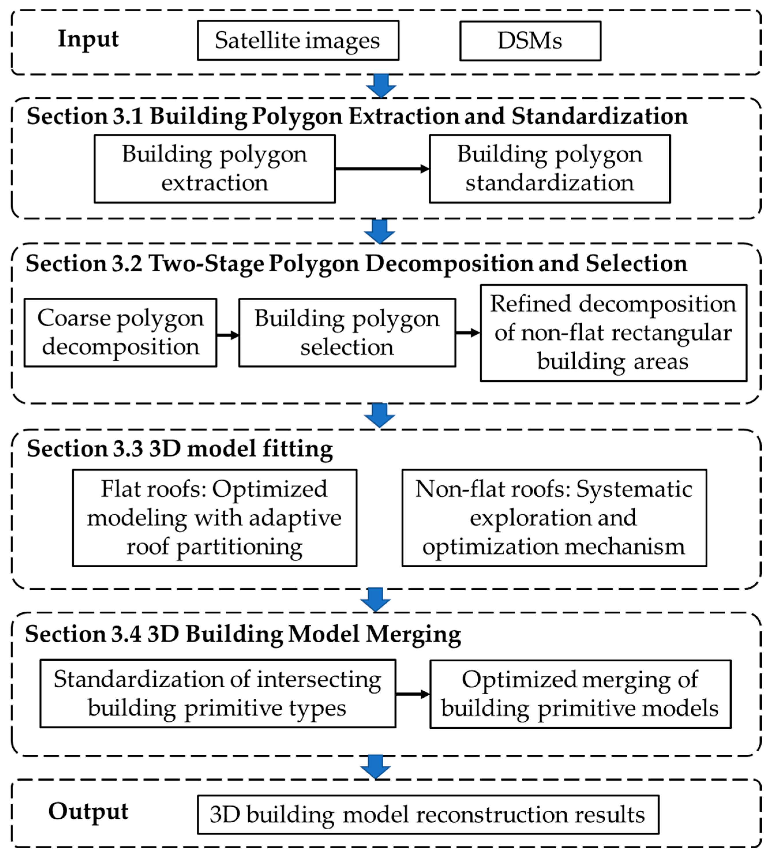
Figure 1. The flowchart of the research methodology.
Remotesensing 17 03832 g001
Figure 2. Standardization of building polygons. (a) Minor kink detection and structural smoothing, (b) contour regularization by orientation, (c) short-edge regularization, (d) merging co-oriented segments with small offsets. The dashed lines indicate horizontal and vertical directions or serve as reference markers, while the red lines highlight retained line segments.
Remotesensing 17 03832 g002
Figure 3. Two-stage building polygon decomposition and selection pipeline. The solid boxes denote the decomposed rectangles, while the red lines indicate the selected substructure boundaries.
Remotesensing 17 03832 g003
Figure 4. Roof types and geometric parameters.
Remotesensing 17 03832 g004
Figure 5. Experimental parameter analysis across different datasets. (a1a5) Beijing-3, (b1b5) US3D, (c1c5) SuperView-1.
Remotesensing 17 03832 g005aRemotesensing 17 03832 g005b
Figure 6. Standardization results of building polygons. (a1a5) Satellite image, (b1b5) building mask, (c1c5) regularized building polygon.
Remotesensing 17 03832 g006
Figure 7. Building polygon decomposition results. (a1a4) Ground truth (GT), (b1b4) ours, (c1c4) Gui, (d1d4) Partovi. The red boxes denote the decomposed rectangles.
Remotesensing 17 03832 g007
Figure 8. Visualization of 3D building reconstruction results. (a1a6) Satellite image, (b1b6) ground truth (GT), (c1c6) ours, (d1d6) ALOD2MR, (e1e6) ABMR, (f1f6) PLANES4LOD2, (g1g6) SAT2LOD2, (h1h6) RDISCMR, (i1i6) FusedSeg-HE.
Remotesensing 17 03832 g008
Figure 9. Visualizations of our method on complex and diverse buildings. (a1a3) Satellite image, (b1b3) ground truth (GT), (c1c3) ours.
Remotesensing 17 03832 g009
Table 1. Optimization parameter search range and step size.
ParameterSearch RangeStep Size
Z e a v e ( Z e a v e ( 0 ) 3 , Z e a v e ( 0 ) + 3 ) 0.2
Z r i d g e ( Z e a v e + 0.5 , Z e a v e + 4 ) 0.2
h i p l ( h i p l ( 0 ) 1 / 8   L , h i p l ( 0 ) + 1 / 8   L ) 0.4
h i p w ( h i p w ( 0 ) 1 / 8   W , h i p w ( 0 ) + 1 / 8   W ) 0.4
Table 2. IOU2 and IOU3 for building polygon decomposition methods.
Method/
Building Target
PartoviGuiOur
1IOU20.80220.90330.9067
IOU30.77330.90230.9284
2IOU20.91900.91900.9190
IOU30.89130.89130.8991
3IOU20.92240.89370.9224
IOU30.89390.84280.9140
4IOU20.89620.85190.8962
IOU30.85470.82840.8609
Table 3. Quantitative evaluation of 3D building reconstruction results.
Method/
Building Target
OurALOD2MRABMRPLANES4
LOD2
SAT2LOD2RDISCMRFusedSeg-HE
1IOU3 (%)86.0979.5183.6280.2877.3578.6878.42
RMSE (m)0.511.220.611.361.491.291.34
MHE (m)0.130.180.320.250.170.280.30
2IOU3 (%)92.4785.4480.3591.8283.8088.1686.87
RMSE (m)1.673.573.683.263.592.743.09
MHE (m)0.401.441.600.721.510.690.75
3IOU3 (%)89.9186.0084.3687.3186.0986.4186.24
RMSE (m)0.390.440.470.410.450.430.47
MHE (m)0.230.260.270.240.260.250.28
4IOU3 (%)91.4079.7786.2787.6581.7886.7487.19
RMSE (m)0.541.290.670.921.301.030.96
MHE (m)0.200.310.240.260.290.270.25
5IOU3 (%)91.0086.6785.4187.9586.2187.2287.63
RMSE (m)0.581.451.591.241.481.291.27
MHE (m)0.260.330.300.400.290.450.42
6IOU3 (%)92.8490.1176.2292.2986.5589.4288.36
RMSE (m)1.191.433.411.321.381.341.48
MHE (m)0.180.300.630.200.480.270.33
Table 4. Quantitative evaluation of averaged 3D building reconstruction results.
MethodOurALOD2MRABMRPLANES4
LOD2
SAT2LOD2RDISCMRFusedSeg-HE
IOU3 (%)91.2685.5483.1788.3683.6886.3285.89
RMSE (m)0.781.491.711.351.601.371.41
MHE (m)0.220.450.540.320.510.360.37
Table 5. Quantitative evaluation of the proposed method on degraded data.
MetricOriginal DataResolution
Reduction
Noise
Injection
Occlusion
IOU3 (%)91.4290.8791.2391.34
RMSE (m)0.750.890.800.77
MHE (m)0.210.240.220.21
Disclaimer/Publisher’s Note: The statements, opinions and data contained in all publications are solely those of the individual author(s) and contributor(s) and not of MDPI and/or the editor(s). MDPI and/or the editor(s) disclaim responsibility for any injury to people or property resulting from any ideas, methods, instructions or products referred to in the content.