An SSA-SARIMA-GSVR Hybrid Model Based on Singular Spectrum Analysis for O3-CPM Prediction

Highlights

What are the main findings?

• SSA-SARIMA-GSVR demonstrates superior performance over benchmark models.
• Reconstruction Threshold (RT) enabling intelligent trend-noise separation for enhanced accuracy.

What is the implication of the main finding?

• Versatile forecasting framework for complex time series across multiple fields.
• Reliable predictive tool for mesospheric ozone with high practical value in atmospheric research.

Abstract

Ozone density at cold-point mesopause (O3-CPM) can provide information on long-term atmospheric trends. Compared to ground-level ozone, O3-CPM is not only adversely affected by chemical substances emitted from human activities but is also regulated by solar radiation. Therefore, an accurate prediction of O3-CPM is necessary. However, it is difficult for traditional forecasting methods to predict the main trends and seasonal characteristics of ozone time series while capturing the random components and noise of O3-CPM. In order to improve the prediction accuracy of O3-CPM, this paper proposes a hybrid SSA-SARIMA-GSVR model based on the Singular Spectrum Analysis (SSA) method, which combines the Seasonal Autoregressive Integrated Moving Average Model (SARIMA) and the Gray Wolf Algorithm Optimized Support Vector Regression Algorithm (GSVR). First, the O3-CPM sequence is decomposed using SSA, and the concept of reconstruction threshold (RT) is introduced to categorize the decomposed singular values into two classes. The categorized RT reconstructed sequences containing periodic features and major trends are fed into the SARIMA model for prediction, and the N-RT reconstructed sequences (original sequence N minus RT reconstructed sequence) containing stochastic components and nonlinear features are fed into the GSVR model for prediction. The final prediction results are obtained by superimposing the outputs of these two models. The results confirm that, compared to various commonly used time series forecasting models such as Long Short-Term Memory (LSTM), Informer, SVR, SARIMA, GSVR, SSA-GSVR, and SSA-SARIMA models, the proposed SSA-SARIMA-GSVR hybrid prediction model has the lowest error evaluation metrics, enabling accurate and efficient prediction of the O3-CPM time series. Specifically, the proposed model achieved an RMSE of 0.26, MAE of 0.212, and R² of 0.987 on the test set, outperforming the best baseline model (SARIMA) by 45.8%, 42.1%, and 3.1%, respectively.

1. Introduction

Ozone, a common air pollutant, is produced by a series of complex photochemical reactions, and severe ozone pollution can be extremely destructive to both human health and the ecological balance. Unlike the pattern of production and change in ozone at the surface, ozone distributed in the mesosphere is not only susceptible to the dynamics of the upper and lower atmosphere, but it is also considered to be an atmospheric factor that is susceptible to active change by human influence.

Ozone at the cold-point mesopause (O3-CPM) refers to the ozone concentration near the mesopause region, which is the boundary layer between the mesosphere and the thermosphere. This region plays a critical role in atmospheric radiative balance and chemical processes, influencing both climate dynamics and space weather. O3-CPM is particularly sensitive to solar ultraviolet radiation and atmospheric circulation patterns, making it a valuable indicator for studying long-term atmospheric changes and anthropogenic impacts on the upper atmosphere.

Therefore, accurate prediction of ozone is important for reducing greenhouse gas emissions and maintaining ecological balance [1]. Specifically, predicting O3-CPM is essential for understanding the coupling processes between different atmospheric layers, assessing the impact of space weather on Earth’s environment, and evaluating the long-term effects of human activities on the upper atmosphere. The variation in O3-CPM is driven by multiple factors, including solar cycle activity, atmospheric wave dynamics, temperature fluctuations, and chemical interactions with species such as atomic oxygen and hydrogen. Moreover, increasing evidence suggests that anthropogenic emissions, such as greenhouse gases and halocarbons, can indirectly affect mesospheric ozone through changes in atmospheric temperature and circulation.

However, ozone at the mesopause region is influenced by various factors and is actively involved in complex chemical reactions, making the prediction of O3-CPM a challenging task. The variation in O3-CPM is driven by multiple factors, including solar cycle activity, atmospheric wave dynamics, temperature fluctuations, and chemical interactions with species such as atomic oxygen and hydrogen. Moreover, increasing evidence suggests that anthropogenic emissions, such as greenhouse gases and halocarbons, can indirectly affect mesospheric ozone through changes in atmospheric temperature and circulation [1,2]. For instance, rising CO₂ levels lead to mesospheric cooling, which may alter O₃ production and loss rates. Therefore, a considerable amount of research has been devoted to ozone prediction in the troposphere [3,4,5,6,7], while there is relatively little research on predicting O3-CPM. Recent studies have further explored the dynamics of mesospheric ozone and the application of hybrid models [8,9,10], highlighting the growing recognition of the complex interplay between solar activity, atmospheric chemistry, and anthropogenic influences in the mesosphere. Since machine learning algorithms can achieve good prediction results with high computational efficiency based on a small amount of input data [11], more and more machine learning models have been applied to forecast variations in ozone.

Traditional machine learning models have good predictive ability for nonlinearly varying data, and many scholars have used these models for ozone prediction. For example, [12] have discussed the potential of using random forest and RNN models to replace traditional atmospheric prediction models. The reliability of support vector machines in predicting ozone changes has also attracted the attention of several scholars [13,14]. Additionally, machine learning models such as recurrent neural networks (RNNs), artificial neural networks [15], long- and short-term memory (LSTM) [16], and seasonal autoregressive integral moving average (SARIMA) [17,18,19,20] have been widely used in ozone prediction. Although these machine-learning models offer significant advantages over traditional statistical models for ozone prediction [21,22], a common drawback is their reliance on a single model. When the influencing factors are complex, the accuracy of these prediction models may decrease over longer periods of time [23]. Therefore, linear or nonlinear combinatorial models based on multiple models are favored by most scholars. By integrating different models that capture various aspects of the data, the overall performance can often be enhanced [24]. Numerous studies have demonstrated that breaking down a complex problem into multiple manageable subproblems through hybrid models can simplify the modeling process while enhancing prediction accuracy and model robustness. In the study by [5], the original ozone sequences were first broken down using full ensemble empirical mode decomposition (CEEMD), then predicted using an optimized hybrid model, effectively overcoming the limitations of a single model and enhancing prediction accuracy. Time series of meteorological factors often exhibit unpredictable and stochastic components due to seasonal changes and unexpected events, such as human activities. Therefore, prediction models that excel at capturing periodic trends and stochastic components tend to achieve high prediction accuracy [25,26,27,28]. In addition, ref. [29] verified the effectiveness of long- and short-term memory networks based on multistage differential embedding in capturing the linear trend and periodicity of time series by predicting surface ozone concentration. Ref. [30] hybridized the SARIMA and SVM models, and the hybrid model took into account the ability to deal with both linear and nonlinear features, which effectively improved the prediction accuracy of ozone.

This paper proposes a hybrid SSA-SARIMA-GSVR prediction model for forecasting O3-CPM based on the traditional decomposition and combination approaches. The SSA method is utilized to extract various components from the original sequence. Subsequently, the concept of RT reconstruction is introduced to facilitate the secondary categorization of components with distinct characteristics. In order to fully consider the seasonal cyclic variation characteristics and major trends of the O3-CPM time series, the SARIMA model was selected to target the prediction of the RT reconstructed series. Considering the excellent potential of the SVR model optimized by the Gray Wolf algorithm in capturing the stochastic components and the noise in the sequences, the GSVR model was applied to predict the N-RT reconstructed sequences. The final comparison of the prediction results of the hybrid model with the single or dual hybrid models found that the SSA-SARIMA-GSVR hybrid model utilized the respective advantages of the SARIMA and GSVR models without significantly increasing the computation time, and provided high-precision prediction results for the prediction of O3-CPM. Additionally, all experiments were conducted using conda 23.7.4 and Python 3.11.

2. Research Methodology

2.1. Singular Spectrum Analysis

Singular Spectrum Analysis (SSA) is a method capable of handling nonlinear time series data by employing Singular Value Decomposition (SVD) on a specific matrix constructed from the time series. The raw time series data is broken down into its most basic elements by this procedure, which includes trend, noise, and oscillatory components. Subsequently, these components are analyzed and reconstructed based on the specific requirements of the task. Unlike parametric models, SSA does not rely on assumptions regarding model parameters or smoothness conditions, making it widely applicable in various fields such as meteorology [31], oceanography [32], economics [33], and astronomy [34]. SSA can be specifically divided into two stages, which are decomposition and reconstruction [35]. Each of the two stages contains two separate steps; in the decomposition stage, the two steps are embedding and singular value decomposition (SVD), and in the reconstruction phase, the two steps are grouping and reorganization.

The decomposed components from SSA form the foundation of our hybrid model. The subsequent introduction of the Reconstruction Threshold (RT) in Section 3 allows us to strategically group these components into meaningful subsets (RT and N-RT sequences) for targeted prediction by the most suitable models.

• Decomposition

The first step in decomposition is embedding, a window length l is selected to lag-arrange the original one-dimensional time series data $[x_1, x_2, x_3,..., x_n]$, forming its trajectory matrix X. In this matrix, the rows correspond to the data points, the columns represent various time delays, and the condition $2\le l\le n/2$ is typically satisfied, where $n$ denotes the length of the time series.

$$X=\left[\begin{array}{cccc}{x}_1& x_2& \dots & x_{n-l+1}\\ x_2& x_3& \dots & x_{n-l+2}\\ \dots & \dots & \dots & \dots \\ x_l& x_{l+1}& \dots & x_n\end{array}\right]$$

(1)

The second step is the singular value decomposition (SVD). The trajectory matrix $X{X}^T$ undergoes SVD, taking the form $X{X}^T=UE{V}^T$. Here, U and $V^T$ represent the left and right singular matrices, respectively, and E is a diagonal matrix containing the singular values along its diagonal. Following the decomposition, the matrix is decomposed to obtain the eigenvalues ${\lambda }_1\ge ...\ge {\lambda }_I\ge 0$ and their corresponding eigenvectors U₁, U₂, ..., U₁, Ultimately, the matrix X is reconstructed using $X=\sum _{i=1}^l\sqrt{{\lambda }_i}{U}_i{V}_i^T,V_i=X^T{U}_i/\sqrt{{\lambda }_i}, i=1,2,...,l$.

Intuitively, this step identifies the dominant patterns (e.g., trends, cycles) in the time series. Each eigenvalue ${\lambda }_i$ represents the energy or importance of its corresponding pattern, with larger eigenvalues indicating more significant components.

2.

Reconstruction

The grouping step involves splitting and summing the matrices obtained in the singular value decomposition step, and the result of the reorganization is that the trajectory matrix is expressed as the sum of several resultant matrices. The singular value decomposition of X of the trajectory matrix can be defined by dividing $i=1,...,l$ into $I_1,I_2,...,I_M$:

$$X_I=X_{I_1}+X_{I_2}+,...,+X_{I_m}$$

(2)

The reorganization step is to aggregate the reorganized results matrix into a new time series, specifically transforming each matrix $X_{I_j}$ in Equation (2) into a new sequence of length n, Let Y be a l*K matrix with matrix elements $y_{ij}$, $1\le i\le \mathrm{l},1\le j\le K$. Let $l^{*}=min(l, K)$, $K^{*}=max(l,K)$, $n=\mathrm{l}+K-1$ if $l<K$, $y_i{j}^{*}=y_{i}j$, otherwise $y_i{j}^{*}=y_{i}i$, and use the following equation to transform the matrix Y is converted to the sequence $(y_1,y_2,\mathrm{\dots },y_n)$.

$$y_k=\left\{\begin{array}{l}{\displaystyle \frac{1}{k}}{\displaystyle {\sum }_{m=1}^k{y}_{m,k-m+1}^{*}},1\le k<l^{*}\\ {\displaystyle \frac{1}{l}}{\displaystyle {\sum }_{m=1}^{l^{*}}{y}_{m,k-m+1}^{*},l^{*}\le k\le K^{*}}\\ {\displaystyle \frac{1}{n-K+1}}{\displaystyle {\sum }_{m=k-K^{*}+1}^{n-K^{*}+1}{y}_{m,k-m+1}^{*},K^{*}<k\le n}\end{array}\right.$$

(3)

2.2. SARIMA Model

The SARIMA model, derived from the ARIMA model, incorporates a seasonal influence component [36] and is represented in a generalized multiplicative form as $(p,d,q)\times (P,D,Q,s)$. Its mathematical formulation is given by: $\mathsf{\varphi }\left(\mathrm{B}\right)\mathsf{\Phi }({\mathrm{B}}^{\mathrm{S}}){(1 - \mathrm{B})}^{\mathrm{d}}{(1 - {\mathrm{B}}^{\mathrm{S}})}^{\mathrm{D}}{\mathrm{y}}_{\mathrm{t}}=\mathsf{\theta }\left(\mathrm{B}\right)\mathsf{\Theta }({\mathrm{B}}^{\mathrm{S}}){\mathsf{ϵ}}_{\mathrm{t}}$. SARIMA is often preferred over the ARIMA model for forecasting time series with cyclical or seasonal features [37]. In our hybrid framework, the SARIMA model is specifically employed to forecast the RT-reconstructed sequence, which contains the smoothed major trends and seasonal cycles extracted by SSA. This leverages SARIMA’s strength in modeling linear, periodic patterns. Its modeling process involves the following steps:

• Plot the original data’s time series and conduct a unit root test to assess its smoothness. Smooth sequence can be directly tested for white noise.
• Perform differencing on non-smooth sequence to remove seasonal and trend terms.
• Conduct a unit root test on the resulting smooth sequences to examine for white noise.
• If the sequence pass the white noise test, proceed with ARIMA modeling. The model is ordered based on autocorrelation and partial correlation plots, and optimal parameters are determined using the Akaike Information Criterion (AIC) $(p,d,q)\times (P,D,Q,s)$.
• Utilize the optimal parameters to establish the SARIMA forecasting model. Conduct residual tests to ensure model stability and use the model to forecast the O3-CPM sequence.

2.3. GSVR Model

Finding the parameter configuration that maximizes the SVR model’s prediction accuracy is the main notion underlying GSVR. To do this, the Support Vector Regression (SVR) model’s ideal collection of three critical hyperparameters is found by applying the Gray Wolf Optimization (GWO) algorithm: the penalty factor c, the maximum allowable error $\epsilon$, and the kernel function system g. The GSVR model is tasked with predicting the complex, nonlinear, and stochastic components contained within the N-RT sequence. The GWO algorithm automates the tedious process of hyperparameter tuning, ensuring the SVR model is optimally configured for this specific task.

2.3.1. Support Vector Regression Model

As a supervised learning algorithm, the SVR model optimizes the model by minimizing structural risk and exhibits significant advantages in handling nonlinear, high-dimensional, and small-sample data (Ma et al., 2003) [38]. It is particularly sensitive in capturing the correlation between inputs and outputs, making the SVR model well-suited for processing high-dimensional data. In a given training sample, $x=(x_1,x_2,\mathrm{\dots },x_n)$ where the output value $y_i\in R^n$, it can be computed by a linear function $f(x)$. The correlation between the inputs and the outputs can be expressed as in the following equation:

$$f(x)=w\phi (x)+b$$

(4)

Among them $w\in R^{\mathrm{n}}$, denote the weight vector and the bias vector, respectively. $\phi (x)$ is termed as a transfer function utilized for mapping raw data into a higher-dimensional space. Based on the principle of minimizing structural risk, w and b are determined using the following method:

$$\mathrm{Minimize}:\left[{\displaystyle \frac{1}{2}}|| w|{|}^2+c{\displaystyle \sum _{i=1}^n{\xi }_i}+{\xi }_i^{*}\right]\mathrm{Subject} \mathrm{to}:\left\{\begin{array}{l}{y}_{\mathrm{i}}-(w\phi (x_{\mathrm{i}})+b_{\mathrm{i}})\le \epsilon +{\xi }_{\mathrm{i}}\hfill \\ (w\phi (x_{\mathrm{i}})+b_{\mathrm{i}})-y_{\mathrm{i}}\le \epsilon +{\xi }_{\mathrm{i}}^{*}\hfill \\ {\xi }_{\mathrm{i}},{\xi }_{\mathrm{i}}^{*}\ge 0\hfill \end{array}\right.$$

(5)

where $c$ is a regularization parameter used to balance the model complexity and training error, ${\xi }_i$, ${\xi }_i^{*}$ are non-negative slack variables indicating errors beyond the $\epsilon$. Eventually, the prediction function of SVR is represented as follows:

$$f(x)={\displaystyle \sum _{\mathrm{i} = 1}^n({\alpha }_{\mathrm{i}}-{\alpha }_{\mathrm{i}}^{*})k(x,x_{\mathrm{i}})}+b$$

(6)

where ${\alpha }_i$ and ${\alpha }_{\mathrm{i}}^{*}$ are Lagrange multipliers, and $k(x,x_{\mathrm{i}})$ is the kernel function that maps the input space to a higher-dimensional feature space. To achieve more accurate prediction results, the values of $c$ and $\epsilon$ need to be optimized. Contrast to traditional trial-and-error methods, this paper uses the GWO algorithm to determine suitable parameter values for the SVR model.

In this study, the radial basis function (RBF) kernel was selected for the SVR model due to its flexibility and effectiveness in handling nonlinear relationships. The suitability of the RBF kernel was validated through preliminary experiments comparing its performance with linear and polynomial kernels, where RBF consistently yielded the highest prediction accuracy on the validation set.

2.3.2. Gray Wolf Optimization Algorithm

The GWO algorithm was inspired by wolves’ hunting techniques and was proposed [38]. Gray wolves are divided into four classes in wolf packs: alpha, beta, delta, and omega, forming a hierarchical structure that serves as the basis for the GWO algorithm. The hunting process of wolves consists of three steps: encirclement, pursuit, and attack. The following formula is used to determine the distance between a gray wolf and its victim during the encirclement phase:

$$\overrightarrow{D}=\left|\overrightarrow{C}\cdot {\overrightarrow{X}}_P(t)-\overrightarrow{X}(t)\right|$$

(7)

Here, $t$ represents the iteration number, $\overrightarrow{X}$ and ${\overrightarrow{X}}_P$ represent the position vectors of the gray wolf and the prey, respectively. Therefore, the position update formula for the gray wolf is given by:

$$\overrightarrow{X}\left(\begin{array}{c}t+1\end{array}\right)={\overrightarrow{X}}_p\left(\begin{array}{c}t\end{array}\right)-\overrightarrow{A}\cdot \overrightarrow{D}$$

(8)

Here, $\overrightarrow{A}\cdot \overrightarrow{D}$ represents the range within which the gray wolves encircle the prey, $\overrightarrow{A}$ and $\overrightarrow{C}$ are coefficient vectors, and $\overrightarrow{A}=2\overrightarrow{a}\cdot \overrightarrow{r_1}-\overrightarrow{a}$, $\overrightarrow{C}=\overrightarrow{2r_2}$, where $\overrightarrow{r_1}\overrightarrow{,r_2}\in \left[0,1\right]$ are random vectors, and a is the distance control parameter.

During the pursuit process, the characteristics of alpha (representing the potential optimal solution), beta, and delta are utilized to gather information about the prey’s location. This information is then used to guide the movement of omega during iterations, facilitating global optimization.

$$\begin{array}{c}{\overrightarrow{X}}_1={\overrightarrow{X}}_{\alpha }-{\overrightarrow{A}}_1\cdot {\overrightarrow{D}}_{\alpha }\\ {\overrightarrow{X}}_2={\overrightarrow{X}}_{\beta }-{\overrightarrow{A}}_2\cdot {\overrightarrow{D}}_{\beta }\\ {\overrightarrow{X}}_3={\overrightarrow{X}}_{\delta }-{\overrightarrow{A}}_3\cdot {\overrightarrow{D}}_{\delta }\\ \overline{X}(t+1)={\displaystyle \frac{{\overline{X}}_1+{\overline{X}}_2+{\overline{X}}_3}{3}}\end{array}$$

(9)

Here, ${\overrightarrow{X}}_{\alpha }$, ${\overrightarrow{X}}_{\beta }$, ${\overrightarrow{X}}_{\delta }$ and $\overrightarrow{X}$ represent the positions of alpha, beta, delta, and omega, respectively.${\overrightarrow{D}}_{\alpha }$${\overrightarrow{D}}_{\beta }$${\overrightarrow{D}}_{\delta }$ represent the distances between omega and alpha, beta, and delta, respectively. During the position update process, ${\overrightarrow{X}}_1$, ${\overrightarrow{X}}_2$, ${\overrightarrow{X}}_3$ represent the positions to which the omega wolf needs to adjust under the influence of alpha, beta, and delta wolves. The final position of the wolf pack is represented by $\overline{X}(t+1)$. During the iteration process, $\overrightarrow{a}$ decreases from 2 to 0, and $\overrightarrow{A}$ narrows within the interval $[-a,a]$, the gray wolf’s future location can be anywhere between its current position and the prey’s position while $\overrightarrow{A}$ is inside $[-1,1]$. The fitness value in the GWO algorithm is set to the value of the prediction model evaluation index $R^2$, This means the cost function (or fitness function) for the GWO to maximize is the R² value of the SVR model’s prediction on the validation set. The objective is to find the hyperparameter combination that yields the highest possible $R^2$, thereby maximizing the prediction accuracy of the GSVR model for the N-RT sequences. The higher the value of $R^2$, the higher the SVR prediction accuracy and the better the result.

3. Construction of SSA-SARIMA-GSVR Hybrid Model

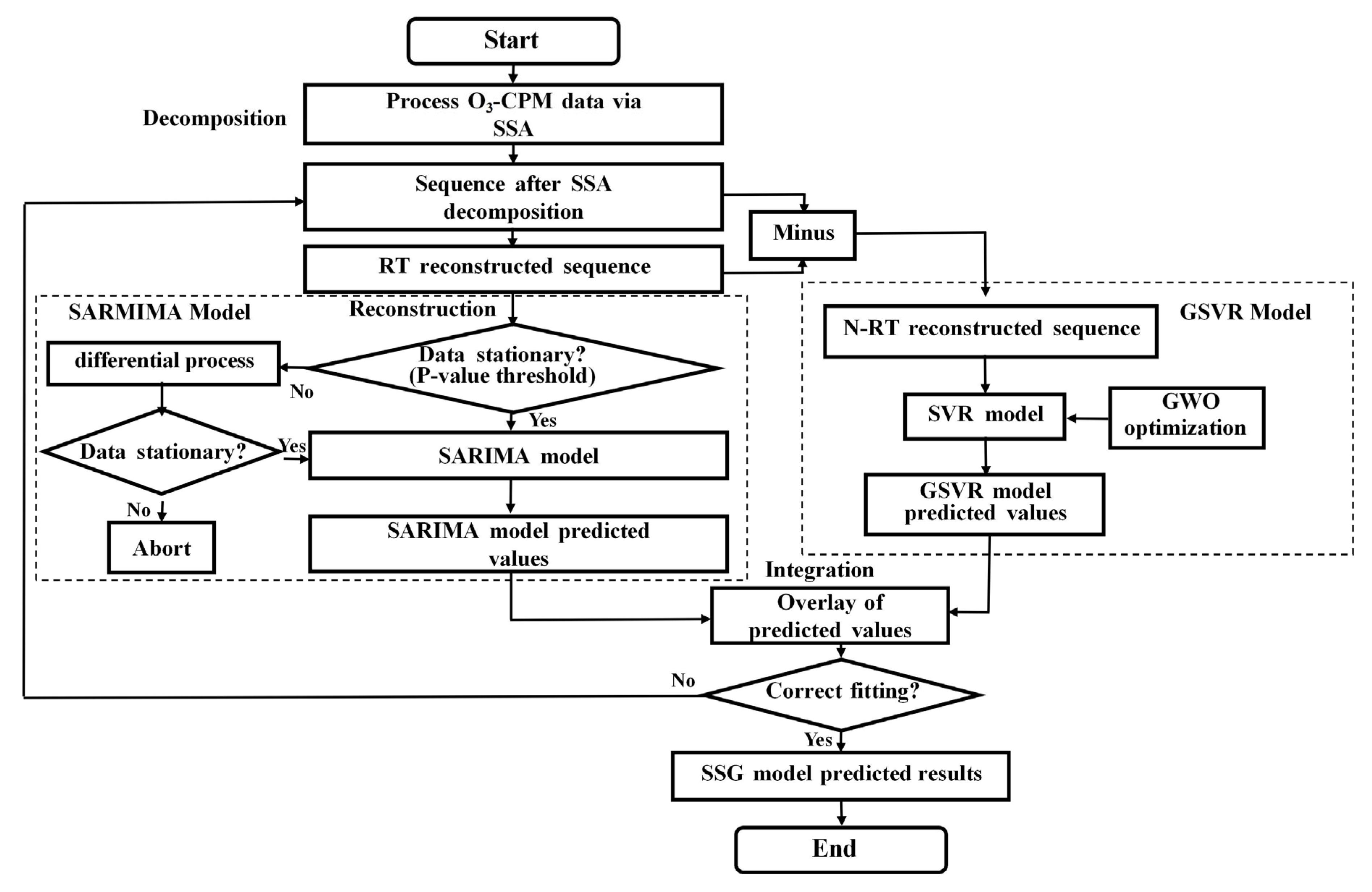
Figure 1 depicts the general structure of the proposed SSA-SARIMA-GSVR hybrid model. Similar to the traditional fusion approach for time series forecasting models, the SSA-SARIMA-GSVR model also follows the logic of decomposition followed by combination.

However, it introduces the concept of a reconstruction threshold (RT) to further categorize the N different components obtained from the SSA decomposition. The Reconstruction Threshold (RT) is defined as the number of leading SSA components whose cumulative contribution to the total variance of the original time series exceeds a predefined threshold (e.g., 99.5%). Formally, if the singular values are ordered as λ₁ ≥ λ₂ ≥ ... ≥ λ_L, then RT is the smallest integer k. The first k components of the SSA decomposition are regarded as the primary components when RT = k.

The noise-reduced RT time series is obtained by reconstructing these components, and the noisy N-RT sequence is obtained by reconstructing the k+1st to Nth components. Since the SARIMA model is proficient at capturing the major trends and periodic components retained in the noise-reduced RT time series, it is used to predict the RT reconstructed series. In addition, a GSVR model of the kernel function is introduced to capture the noise and random components in the N-RT sequences. This method increases the final prediction accuracy of the SSA-SARIMA-GSVR model by enabling more focused predictions of the O3-CPM sequence’s deconstructed components. In this study, the original O3-CPM sequence is decomposed into 11 components using SSA. After analysis, the sequence input to the SARIMA model should be the RT reconstruction sequence of the first eight components, while the sequence input to the GSVR model should be the N-RT reconstruction sequence of the next three components. The best results are acquired by superimposing the outputs from both models to arrive at the final forecast.

4. Datasets and Evaluation Indicators

4.1. Description of the Dataset

The data used in this paper are derived from version 2.0 of the SABER dataset provided by NASA’s TIMED satellite. The primary atmospheric factors analyzed in this study include O3-CPM, temperature (T-CPM), solar activity index (F10.7), hydrogen atom density ([H]-CPM), and oxygen atom density ([O]-CPM). These specific parameters were selected due to their direct physical and chemical relationships with the formation and destruction of mesospheric ozone:

T-CPM: Temperature directly influences the rates of the chemical reactions that govern ozone production and loss.

F10.7: As a proxy for solar extreme ultraviolet (EUV) radiation, it drives the photodissociation of molecular oxygen, which is the primary source of atomic oxygen for ozone production via three-body reactions.

[H]-CPM and [O]-CPM: Hydrogen and oxygen atoms are key participants in the dominant ozone destruction (e.g., H + O₃ → OH + O₂) and production (O + O₂ + M → O₃ + M) cycles in the mesosphere, respectively.

The timeframe for these data spans twenty-two years, from 1 February 2002, to 31 December 2023. The data were collected with an error margin of 0.5 km above and below 95.4 km altitude. The prediction data for this experiment consists of the monthly average values of mesosphere top ozone (O3-CPM) over twenty-two years. Additionally, the monthly average values of other meteorological factors are used as feature inputs to the deep learning Informer prediction model. The dataset from February 2002 to August 2017 (totaling 186 data points) serves as the training set for model development, while the dataset from September 2017 to December 2023 (totaling 77 data points) is used as the validation and testing set for the model.

4.2. Evaluation Indicators

To more accurately and intuitively assess the performance of various models, we have selected seven evaluation metrics: Root Mean Square Error (RMSE), Mean Absolute Percentage Error (MAPE), Mean Absolute Error (MAE), Theil’s Inequality Coefficient (TIC), Sum of Squared Errors (SSE), absolute coefficient (R2), and the Index of Agreement (IA) to analyze the errors of different prediction models. These indexes help analyze the errors of different prediction models. Specifically, the smaller and closer to 0 the RMSE, MAPE, TIC, SSE, and MAE are, the smaller the model’s error is. On the contrary, the larger R2 is, the closer it is to 1, the better the model fits, and the value of IA is closer to 1, the more consistent the model’s prediction is with the real value, and the combination of the two can more comprehensively assess the model’s performance and prediction effect. By using these indicators, the predictive performance of the model can be comprehensively assessed in terms of average error, volatility, and fitting effect. The formulas for these evaluation indexes are shown below [39,40,41,42,43].

$$\mathrm{RMSE}=\sqrt{{\displaystyle \frac{1}{n}}{\displaystyle \sum _{i=1}^n{\left|{\widehat{y}}_i-y_i\right|}^2}}$$

(10)

$$\mathrm{MAPE}={\displaystyle \frac{100\%}{n}}{\displaystyle \sum _{i=1}^n\left|\frac{{\widehat{y}}_i-y_i}{y_i}\right|}$$

(11)

$$\mathrm{MAE}={\displaystyle \frac{1}{n}}{\displaystyle \sum _{i=1}^n\left|{\widehat{y}}_i-y_i\right|}$$

(12)

$${\mathrm{R}}^2=1-{\displaystyle \frac{{\displaystyle \sum _{i=1}^n{\left({\widehat{y}}_i-y_i\right)}^2}}{{\displaystyle \sum _{i=1}^n{\left({\widehat{y}}_i-\overline{y}\right)}^2}}}$$

(13)

$$\mathrm{TIC}={\displaystyle \frac{\sqrt{\frac{1}{n}{\displaystyle \sum _{i=1}^n{\left(y_i-{\widehat{y}}_i\right)}^2}}}{\sqrt{\frac{1}{n}{\displaystyle \sum _{i=1}^n{\widehat{y}}_i^2}}+\sqrt{\frac{1}{n}{\displaystyle \sum _{i=1}^n{y}_i^2}}}}$$

(14)

$$\mathrm{SSE}={\displaystyle \sum _{i=1}^n{\left({\widehat{y}}_i-y_i\right)}^2}$$

(15)

$$\mathrm{IA}=1-{\displaystyle \frac{{\displaystyle \sum _{i=1}^n{\left(y_i-{\widehat{y}}_i\right)}^2}}{{\displaystyle \sum _{i=1}^n{\left(\left|{\widehat{y}}_i-\overline{{\widehat{y}}_i}\right|+\left|{\widehat{y}}_i-\overline{y}\right|\right)}^2}}}$$

(16)

where $n$ is the number of samples, ${\widehat{y}}_i$ is the actual value of the i-th sample, $y_i$ is the predicted value of the i-th sample, $y$ is the mean of the actual values, and $\overline{{\widehat{y}}_i}$ is the mean of the predicted values.

5. Parameter Determination of SSA-SARIMA-GSVR Hybrid Model for O3-CPM Forecasting

5.1. SSA Decomposition and Preliminary Determination of RT Reconstructed Sequences

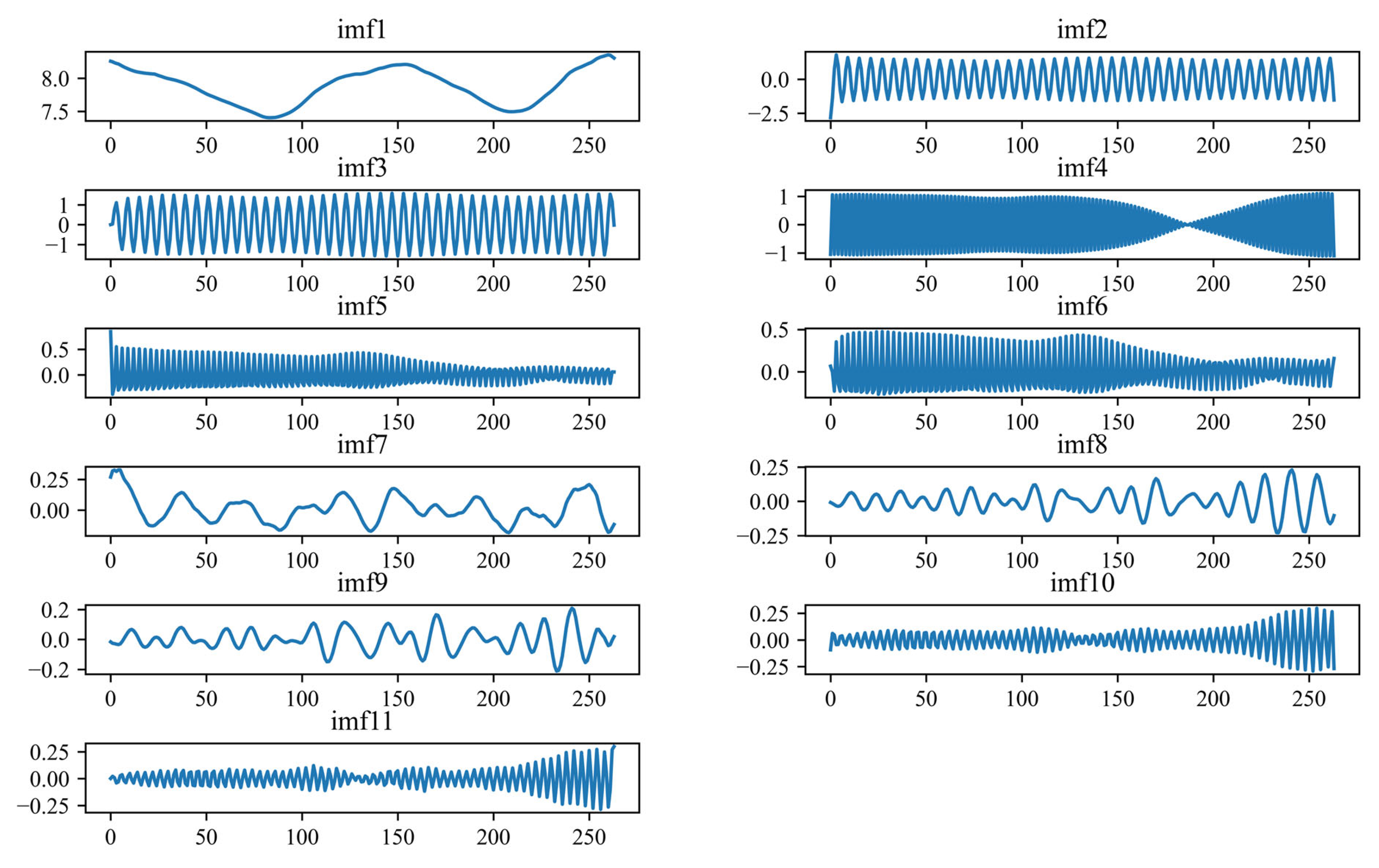
The window value (L) and the number of intrinsic mode functions (IMFs) need to be determined prior to conducting the SSA decomposition of the O3-CPM time series. To effectively capture the periodicity of the O3-CPM sequence while avoiding over-decomposition, the value of L is set to 24, which corresponds to the period of the O3-CPM sequence. This value was chosen because the O3-CPM time series is monthly data, and preliminary spectral analysis (e.g., using Fast Fourier Transform or periodogram) revealed a dominant annual cycle (12 months). In SSA, it is common practice to set the window length L as an integer multiple of the primary period to effectively capture the cyclic behavior; here, L = 2 × 12 = 24 was found to yield a clear separation of components, successfully isolating the annual cycle and its harmonics (see imf2 and imf3 in Figure 2). The 11 components of the SSA decomposition are shown in Figure 2, which are gradual transitions from the main trend and major cyclical components to smaller fluctuations and noise components.

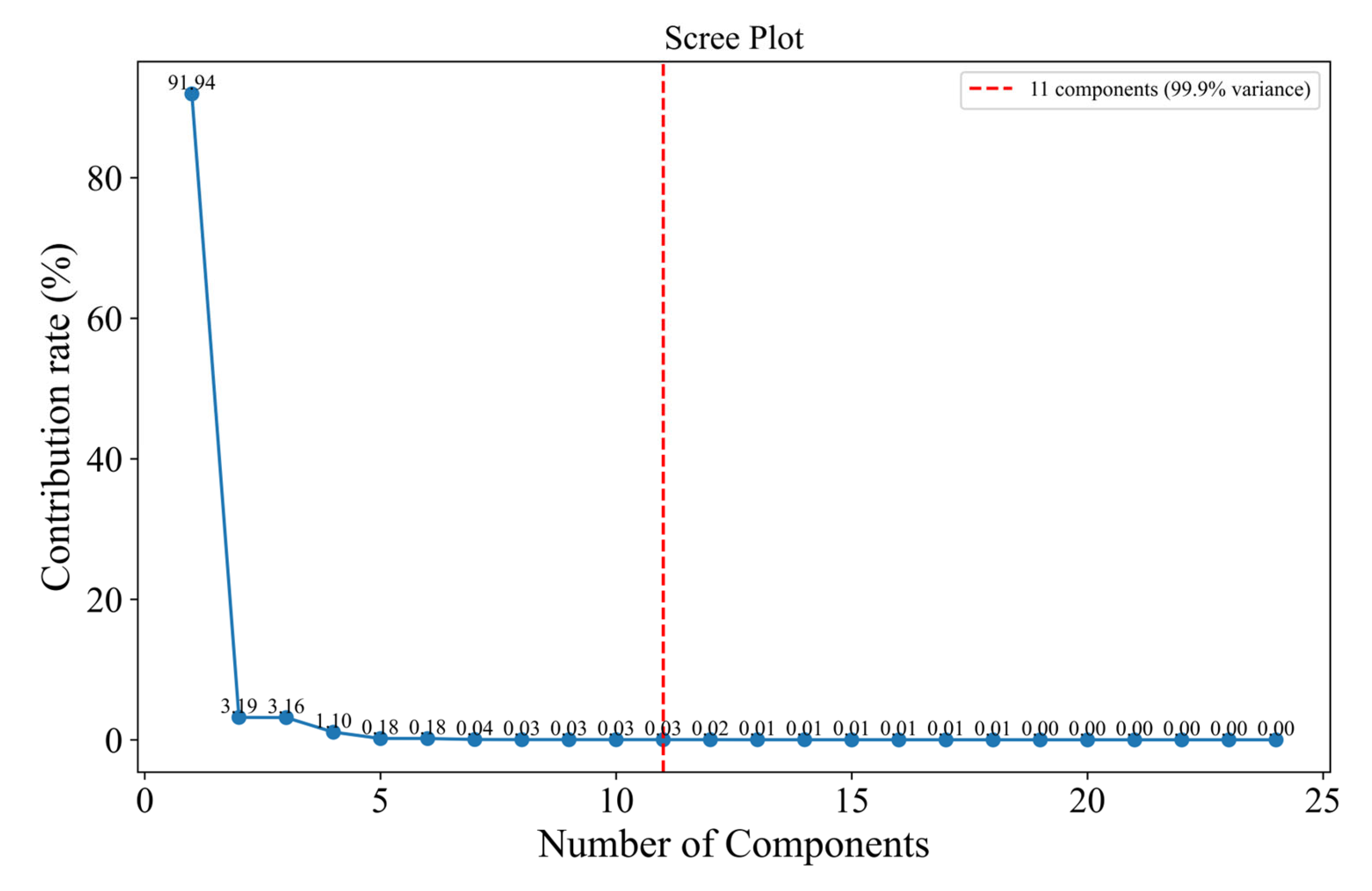
When using SSA for principal component analysis, the components with a contribution rate greater than 95% are generally retained [44], and here, in order to maximize the retention of valid information in the original sequence for the GSVR model while reducing the amount of computation, the maximum contribution rate is set to 99.9%, retaining one decimal place.

A more rigorous method for determining the RT value is to analyze the cumulative contribution rate of the singular values obtained from SVD. The scree plot (Figure 3) visually represents the contribution of each component. The “elbow” point of this curve, where the contribution rate drops significantly, often indicates an optimal cut-off between signal and noise. As seen in Figure 3, a distinct elbow occurs after the 8th component, where the cumulative contribution rate reaches over 99.5%, and the marginal gain from subsequent components becomes negligible. This provides theoretical support for selecting RT = 8, as components beyond this point contribute little information and are primarily stochastic.

As can be seen from Figure 3, the contribution rate of the SSA decomposed components reaches 99.9% at the 11th component, so the first 11 components are selected for reconstruction. Among these components, the characteristics of the first component depict the overall trend of the O3-CPM across 263 consecutive months, contributing 91.94% and thus representing the most significant component of the decomposition. In addition, imf2 and imf3 reflect the seasonal cyclic variation patterns of O3-CPM, while imf4 to imf6 capture the detailed variation characteristics of O3-CPM. Based on this analysis, the components selected for RT reconstruction are preliminary identified as imf1 to imf6 and categorized the remaining imf7 to imf11 totaling 5 components as N-RT reconstruction components.

To formalize the selection of the Reconstruction Threshold (RT) and move beyond preliminary visual inspection, a thresholding rule was applied. The RT was determined as the smallest number of components whose cumulative contribution rate exceeded 99.5% of the total variance, a common criterion in dimensionality reduction. As detailed in Section 5.1 and visualized in the scree plot (Figure 3), the cumulative contribution rate reaches 99.52% at the 8th component. This objective criterion, supported by the distinct “elbow” observed in Figure 3 after component 8, provides a robust and quantitative basis for the selection.

Although the components decomposed by the SSA method can visualize the transition from the main trend to the noise components in the original sequence, the initially determined RT reconstruction threshold may not be accurate. The components corresponding to the RT reconstruction sequence should include the main trend and periodic characteristics of the original sequence, with generally high contribution rates (>0.1%). To effectively reduce the randomness in selecting the RT reconstruction threshold, the SSA decomposition graph and scree plot are used to further determine the RT reconstruction threshold. From the scree plot, it can be seen that the contribution rates of different components start to decrease significantly from the sixth component onward. To determine whether the components after the sixth should be classified into the RT sequence, we set RT = 6, 7, 8, and 9 to reconstruct the decomposed components and perform N-RT reconstruction on the remaining components. The SARIMA model is used to predict the RT reconstruction sequence, and the GSVR model is used to predict the N-RT reconstruction sequence. By comparing the prediction results of models corresponding to different RT values, the most suitable RT and N-RT values are selected.

5.2. SARIMA Model Prediction of RT Reconstructed Sequences

5.2.1. Determination of the Parameters of the SARIMA Model

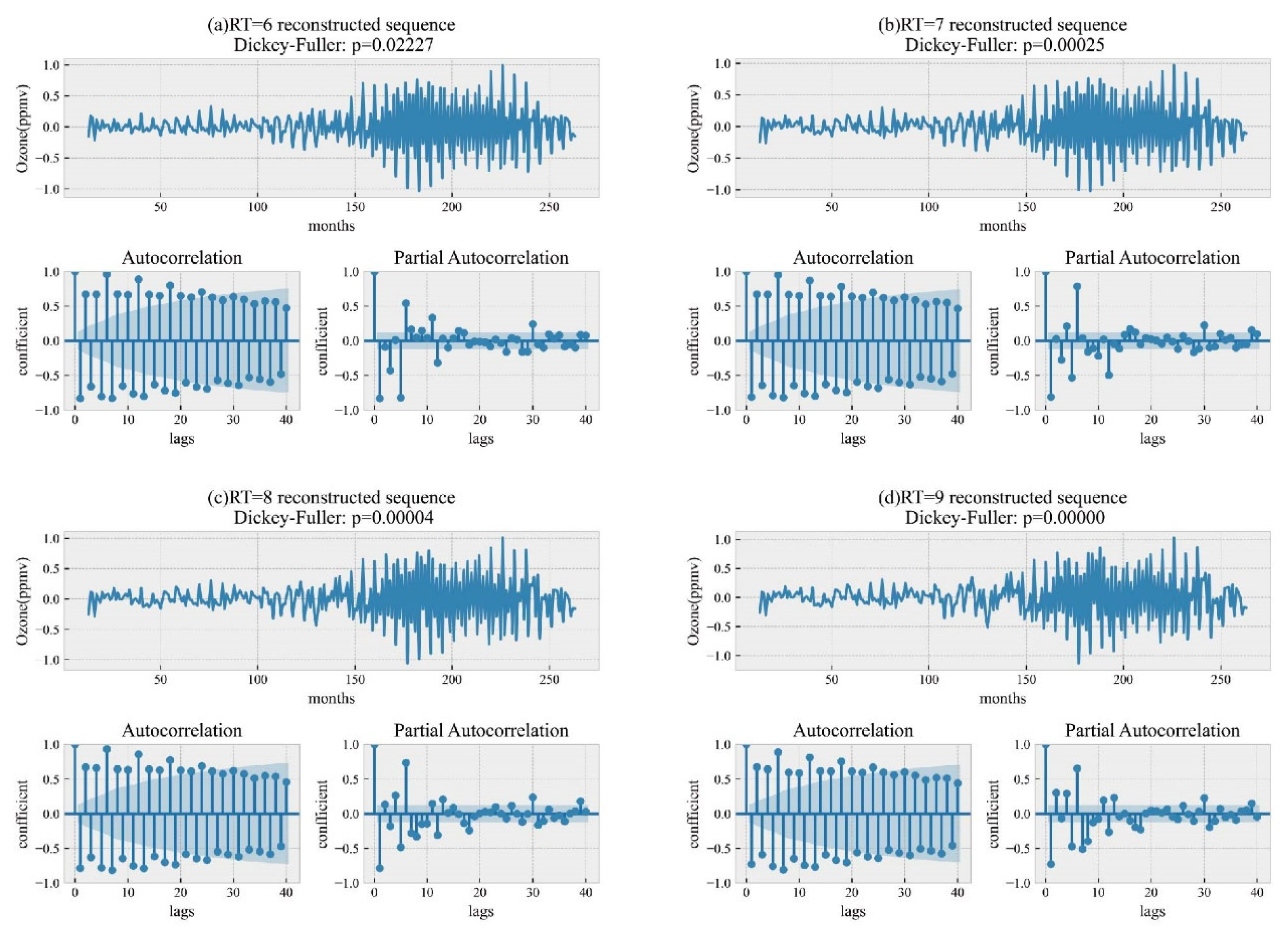
Stationarity is a key factor in whether the SARIMA model can capture the true trends and seasonality of time series data, so it is first necessary to transform the unsmoothed RT reconstructed series into a smooth series. The Augmented Dickey–Fuller (ADF) test is used to determine whether the time series data is stationary. If the p-value is less than 0.05, the null hypothesis is rejected, indicating that the time series is stationary according to the ADF test. The ADF test was conducted on the O3-CPM sequence reconstructed under four different RT values, yielding the following p-values: p-value = 0.00320 < 0.05, p-value = 0.10238 > 0.05, p-value = 0.04350 < 0.05, and p-value = 0.02243 < 0.05. Among these, only the reconstructed sequence with RT = 7 accepted the null hypothesis and was identified as a non-stationary sequence, while the other three RT sequences were all stationary. In order to make the RT = 7 reconstructed sequence smooth, seasonal differencing and first order differencing were applied to it. Figure 4 not only shows the four different RT reconstructed sequences but also presents the autocorrelation and partial autocorrelation plots of these sequences. From the autocorrelation plots of the four RT reconstructed sequences, evident seasonal trends and numerous lags can be observed. Therefore, first-order and seasonal differencing were also applied to the other three reconstructed sequences to ensure stationarity and remove any residual seasonal patterns.

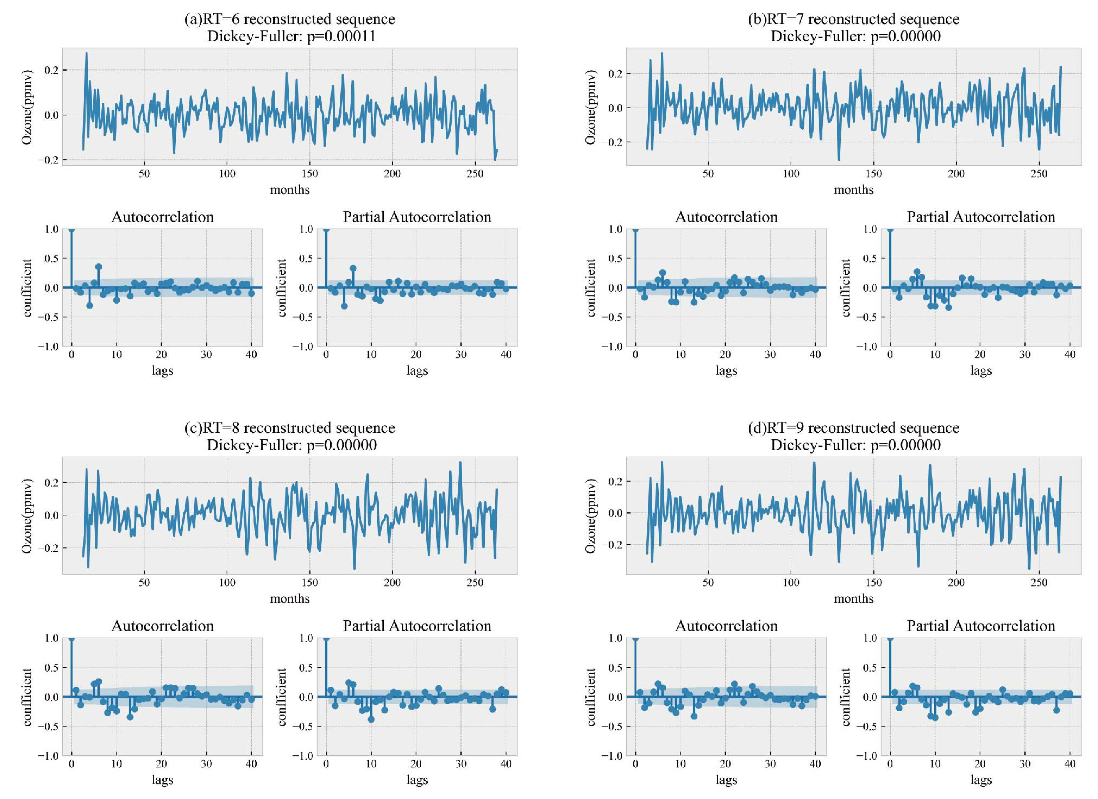
Figure 5 shows the different RT reconstructed sequences obtained after seasonal differencing and first-order differencing, along with their corresponding autocorrelation and partial autocorrelation plots. It can be seen that the seasonal trends in all four reconstructed sequences have been eliminated after processing. The ADF test results for the four RT reconstructed sequences are p-value = 0.02227 < 0.05, p-value = 0.00025 < 0.05, p-value = 0.00004 < 0.05, and p-value = 0.00000 < 0.05, indicating that they have passed the ADF test and have all been transformed into stationary sequences. Here, Ljung–Box test is performed on the reconstructed sequences after differential processing to determine whether the four stationary sequence are white noise, and if the Ljung–Box test value is less than 0.05, the sequences are not considered to be white noise. The corresponding Ljung–Box test results for the reconstructed sequences with RT = 6, 7, 8, 9 are p-value = 6.365807 × 10⁻³⁰⁶ < 0.05, p-value = 4.163243 × 10⁻²⁹⁷ < 0.05, p-value = 1.249973 × 10⁻²⁸⁶ < 0.05, and p-value = 7.194396 × 10⁻²⁶⁵ < 0.05, which are much smaller than 0.05, indicating that all four sequences are not white noise and can be used in the parameterization of SARIMA prediction models determination.

The parameters of the SARIMA prediction model include non-seasonal parameters p, d, q and seasonal parameters P, D, Q, and s. From Figure 5, it can be observed that the autocorrelation coefficients for different RT reconstructed sequences exhibit a tailing trend, while the partial autocorrelation coefficients display a cutting-off characteristic. Specifically, the Autocorrelation Function (ACF) plot shows a slow, exponential decay (tailing off), and the Partial Autocorrelation Function (PACF) plot shows a sharp cut-off after lag p. This pattern is characteristic of an Autoregressive (AR) process, which helps us preliminarily identify the order p. The value of p is determined by the maximum lag value observed from the PACF. For RT = 6 and RT = 7, p values are preliminarily hypothesized to be 4 and 2, respectively. Since a first-order differencing has been applied, d is set to 1. Similarly, the Moving Average (MA) order q would be suggested by an ACF plot that cuts off and a PACF that tails off; however, in our sequences, the AR signature was dominant. The optimal model parameters are ultimately determined using the AIC, where a smaller AIC value indicates a better SARIMA model parameter combination. The AIC values for different RT reconstructed sequences are shown in

Table 1. AIC values corresponding to different parameters in the RT = 6 reconstructed sequence.

Parameters	AIC
SARIMA(2,1,4) × (1,1,1,12)	−602.641265
SARIMA(3,1,4) × (0,1,1,12)	−588.175691
SARIMA(2,1,4) × (0,1,1,12)	−582.565583
…	…
SARIMA(4,1,2) × (0,0,0,12)	−292.510634
SARIMA(3,1,2) × (0,1,0,12)	−286.353925
SARIMA(2,1,2) × (0,1,0,12)	−246.892624

,

Table 2. AIC values corresponding to different parameters in the RT = 7 reconstructed sequence.

Parameters	AIC
SARIMA(3,1,4) × (0,1,1,12)	−440.240990
SARIMA(4,1,3) × (0,1,1,12)	−405.116008
SARIMA(4,1,4) × (0,1,1,12)	−400.207573
…	…
SARIMA(4,1,2) × (0,1,0,12)	−186.298679
SARIMA(3,1,2) × (0,1,0,12)	−157.002676
SARIMA(2,1,2) × (0,1,0,12)	−143.608879

,

Table 3. AIC values corresponding to different parameters in the RT = 8 reconstructed sequence.

Parameters	AIC
SARIMA(3,1,4) × (1,1,1,12)	−377.743125
SARIMA(3,1,4) × (0,1,1,12)	−377.122901
SARIMA(4,1,3) × (0,1,1,12)	−373.195116
…	…
SARIMA(4,1,2) × (0,1,0,12)	−143.491758
SARIMA(3,1,2) × (0,1,0,12)	−125.873274
SARIMA(2,1,2) × (0,1,0,12)	−110.407299

and

Table 4. AIC values corresponding to different parameters in the RT = 9 reconstructed sequence.

Parameters	AIC
SARIMA(4,1,4) × (0,1,1,12)	−352.226182
SARIMA(4,1,4) × (1,1,1,12)	−341.356636
SARIMA(4,1,4) × (1,1,0,12)	−334.405446
…	…
SARIMA(3,1,2) × (0,1,0,12)	−79.439518
SARIMA(2,1,2) × (0,1,1,12)	−4.013588
SARIMA(2,1,2) × (0,1,0,12)	151.267209

.

After determining the parameters, residual diagnostics need to be conducted for the four SARIMA models: SARIMA (2,1,4) × (1,1,1,12), SARIMA (3,1,4) × (0,1,1,12), SARIMA (3,1,4) × (1,1,1,12), and SARIMA (4,1,4) × (0,1,1,12). The diagnostic results are shown in Figure 6, where all the lag values in the PACF plots are almost entirely within the 95% confidence interval shaded area. Therefore, the SARIMA models for the O3-CPM time series reconstructed with RT = 6, 7, 8, and 9 all pass the residual diagnostic tests and are ready for the final step of prediction.

5.2.2. SARIMA Prediction for Different RT Reconstructed Sequences

The SARIMA prediction results for the O3-CPM sequence under different RT reconstructions are shown in Figure 7. It can be observed that the prediction performance of all four RT reconstructed sequences is quite good. The SARIMA model prediction metrics for different RT values are presented in

Table 5. Evaluation metrics for SARIMA prediction of O3-CPM sequence under four RT reconstructions.

	Indicator	RMSE	MAPE (%)	MAE	R2	TIC	IA	SSE
RT Value
RT = 6		0.073	0.007	0.057	0.999	0.004	0.999	0.40
RT = 7		0.106	0.012	0.086	0.998	0.006	0.999	0.85
RT = 8		0.118	0.013	0.094	0.997	0.007	0.999	1.07
RT = 9		0.125	0.014	0.101	0.997	0.008	0.999	1.19

. The prediction errors for the SARIMA models of the four different RT sequences are relatively close, with the SARIMA model for the RT = 6 reconstructed sequence showing slightly better performance compared to the other RT reconstructed sequences. This suggests that the initial determination of the RT reconstruction thresholds in Section 5.1 is reasonable. However, the predictions corresponding to different RT values do not differ significantly, and thus the GSVR should be utilized to predict different N-RT reconstruction sequences to determine the final combination of RT and N-RT.

5.3. GSVR Prediction of N-RT Reconstructed Sequences

5.3.1. Optimization of GSVR Model Parameters

To maximize the prediction accuracy of the SVR model, the GWO algorithm is used for iterative optimization of the model parameters. Figure 8 shows the optimization iteration plots of GSVR for different N-RT reconstructed sequences, with 300 iterations. From Figure 8, the fitness values of the O3-CPM sequence under different N-RT reconstructions quickly reach their maximum within a small number of iterations. This indicates that the improved algorithm accelerates the convergence speed while also preventing the algorithm from falling into local optima, thereby enhancing the robustness of the algorithm to a certain extent.

5.3.2. Prediction of Different N-RT Reconstructed Sequences

The optimal parameters obtained through optimization are substituted into the SVR model for training and prediction. The prediction results for different N-RT reconstructed sequences are shown in Figure 9. As can be seen from Figure 9, the prediction results of the GSVR model for different N-RT reconstruction sequences are not much different. Table 5 presents the prediction evaluation metrics of the GSVR model for N-RT reconstructed sequences with values of 5, 4, 3, and 2. From the metrics in

Table 6. Assessment metrics for GSVR prediction of O3-CPM sequence under four N-RT reconstructions.

	Indicator	RMSE	MAPE (%)	MAE	R2	TIC	IA	SSE
RT Value
N-RT = 2		1.12	0.115	0.867	0.759	0.070	0.912	96.07
N-RT = 3		1.00	0.109	0.811	0.808	0.061	0.942	76.66
N-RT = 4		1.03	0.117	0.866	0.796	0.063	0.944	81.36
N-RT = 5		1.03	0.111	0.845	0.797	0.063	0.945	81.03

, the GSVR prediction performance is best for the N-RT = 3 reconstructed sequence. This result is not consistent with the SARIMA prediction results for the RT reconstructed sequences. Therefore, we will superimpose the different RT and N-RT sequences for the final hybrid model prediction.

5.4. Prediction of SSA-SARIMA-GSVR Model

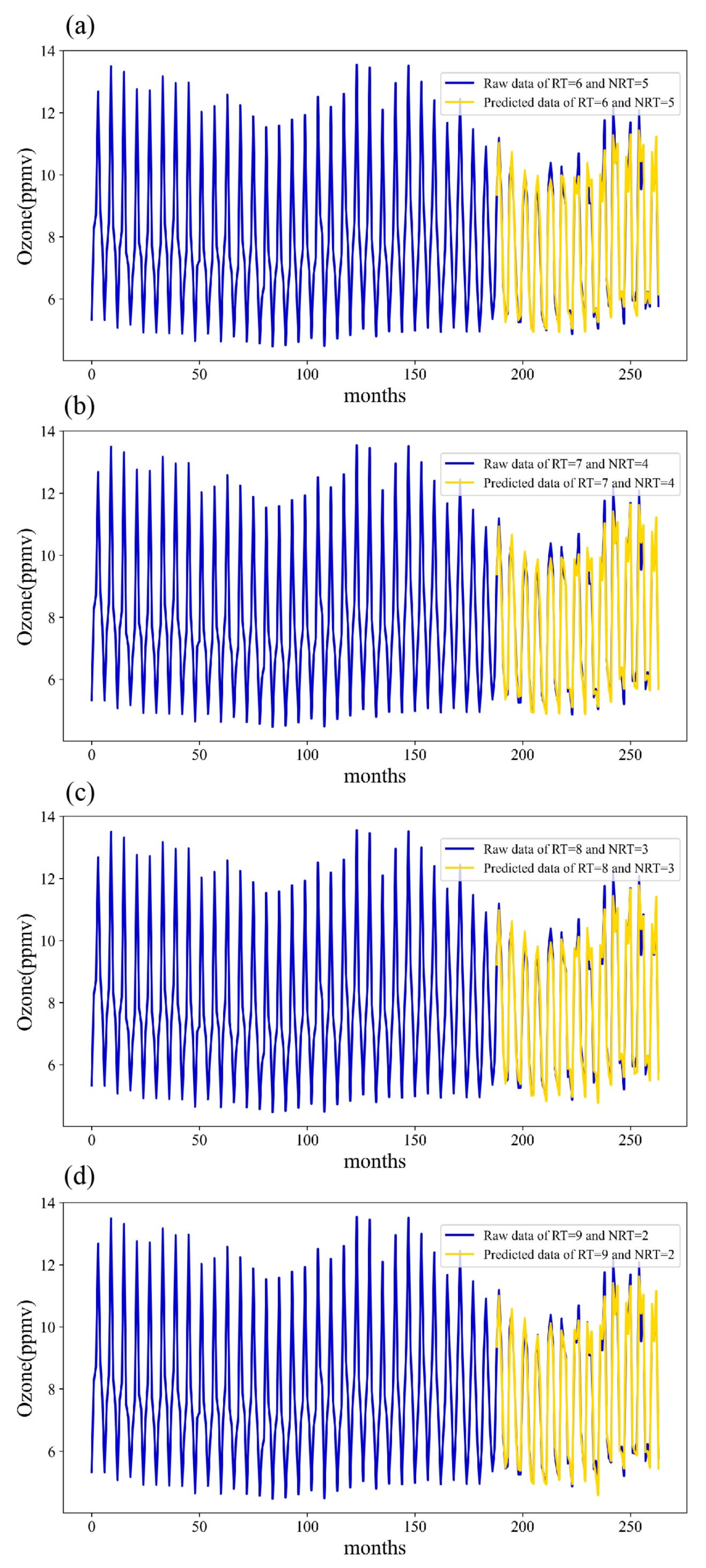
Figure 10 shows the final prediction results of the SSA-SARIMA-GSVR model by superimposing the results of different RT reconstructed sequences and N-RT reconstructed sequences. As can be seen from Figure 10, the superposition results of different RT reconstruction sequences and N-RT reconstruction sequences are very accurate. The evaluation metrics of the SSA-SARIMA-GSVR hybrid model predictions are presented in

Table 7. Evaluation metrics for SSA-SARIMA-GSVR prediction of superposition of four RT and N-RT reconstructed sequences.

	Indicator	RMSE	MAPE (%)	MAE	R2	TIC	IA	SSE
Combination
RT = 6, N-RT = 5		0.36	0.034	0.279	0.975	0.022	0.994	9.88
RT = 7, N-RT = 4		0.32	0.032	0.255	0.980	0.020	0.995	7.96
RT = 8, N-RT = 3		0.26	0.028	0.212	0.987	0.016	0.997	5.18
RT = 9, N-RT = 2		0.33	0.032	0.255	0.980	0.020	0.995	8.08

. A quantitative comparison of the hybrid model’s performance under the four candidate (RT, N-RT) combinations is presented in Table 7, providing the decisive metrics for the final parameter selection.When RT = 8 and N-RT = 3 are superimposed, the SSA-SARIMA-GSVR model has the lowest error among the four results: RMSE = 0.26, MAE = 0.212, TIC = 0.016, SSE = 5.18. Therefore, the parameter value of RT corresponding to the SSA-SARIMA-GSVR model is finally determined to be 8, and the parameter value of N-RT is determined to be 3.

5.5. Comparison of Results of Different Prediction Models

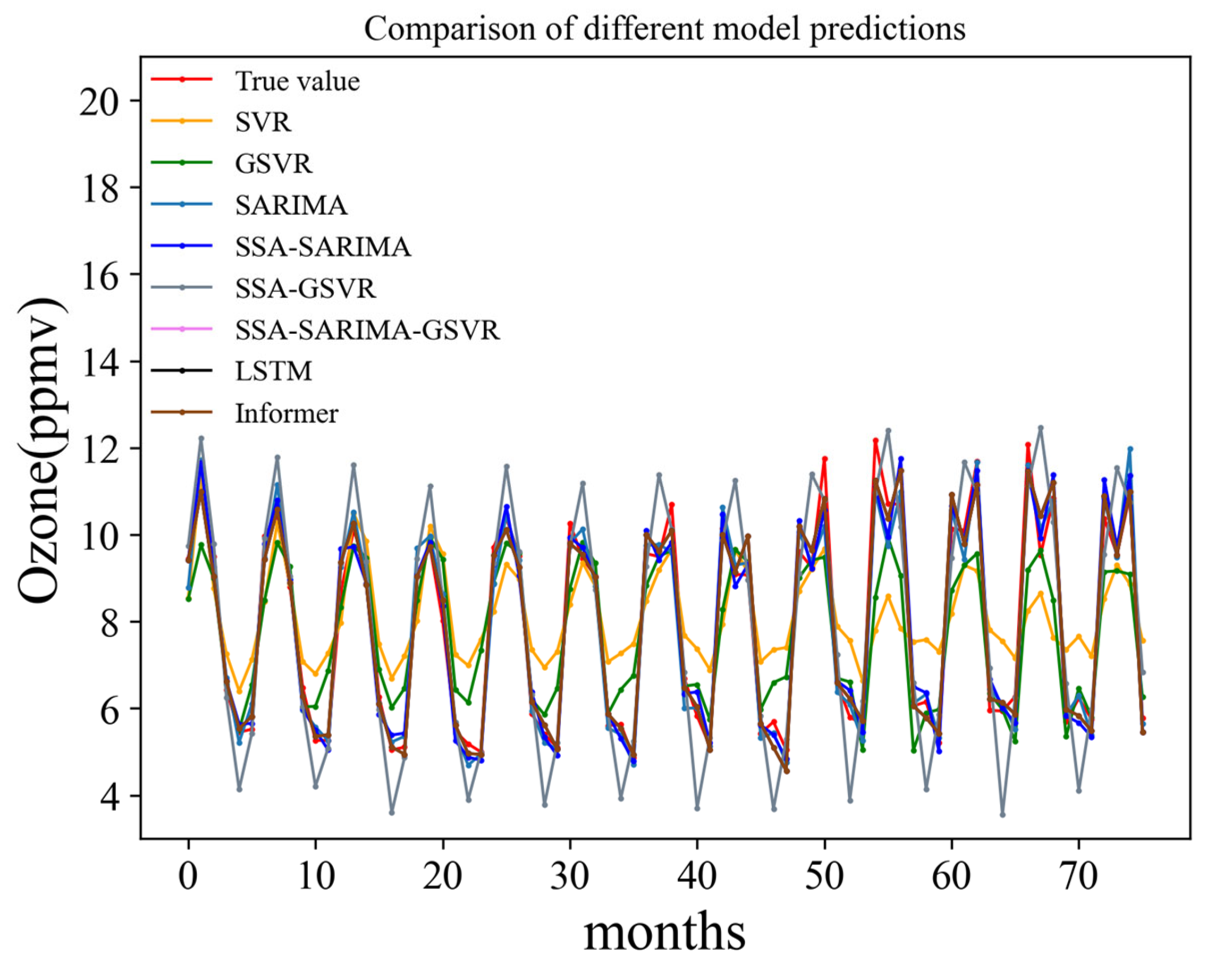
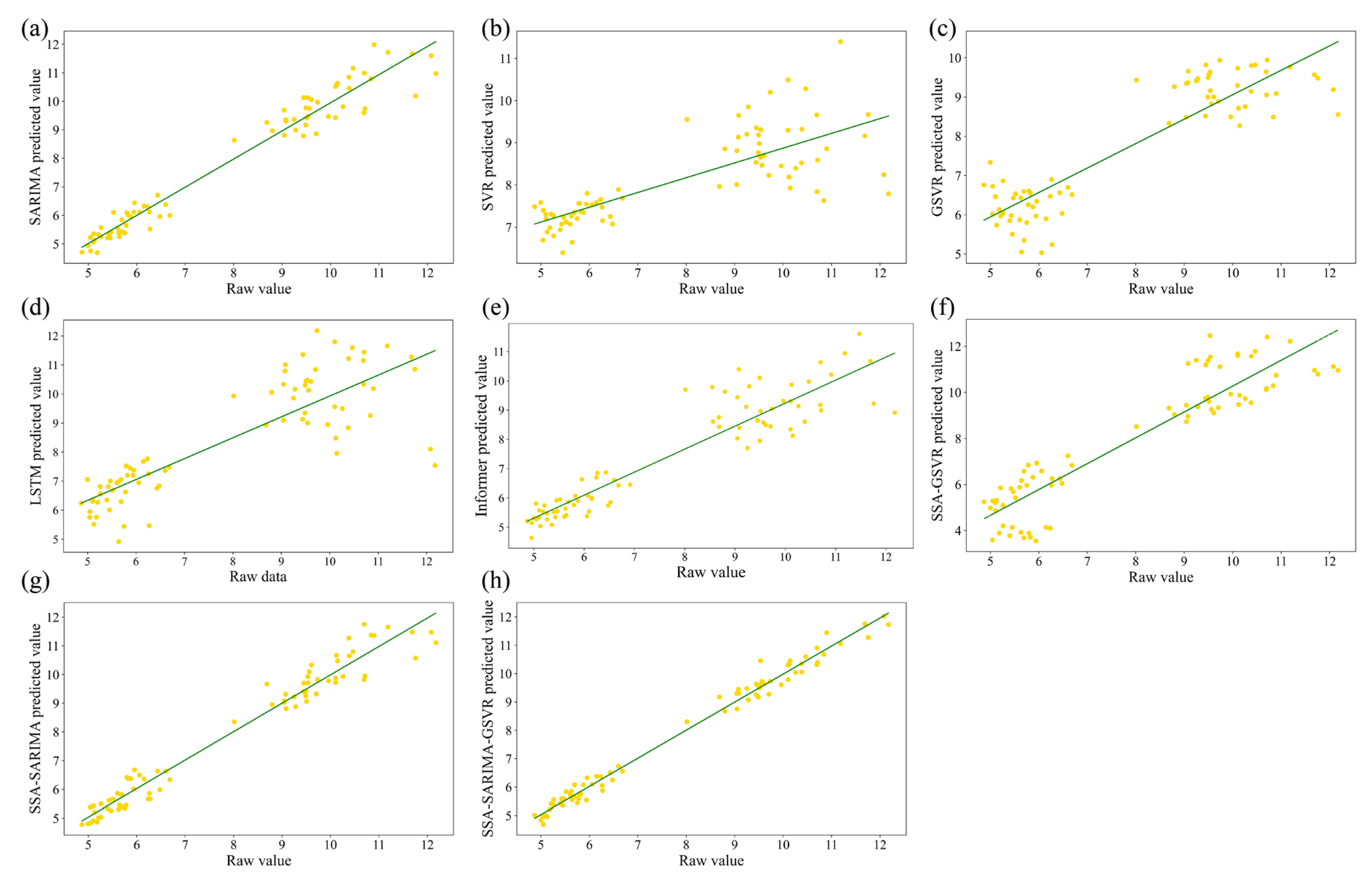
In order to compare the performance of the SSA-SARIMA-GSVR hybrid model with that of single or dual hybrid models and other forecasting models commonly used for time series, the monthly average O3-CPM data are now forecasted using SVR, GSVR, SARIMA, LSTM, Informer, SSA-SARIMA, SSA-GSVR, and the hybrid forecasting model SSA-SARIMA-GSVR, respectively. Figure 11 shows the predicted outcomes of the various models. Figure 12 is a scatter plot depicting the actual and predicted values of various models. It can be observed that in Figure 12h, the actual and predicted values of the SSA-SARIMA-GSVR model cluster closely around the fitting line. This indicates that, compared to other models, the SSA-SARIMA-GSVR model has the highest correlation between the predicted and actual values.

6. Discussion

Due to the SARIMA model’s flexibility in capturing trends and seasonal patterns, it exhibits the best predictive performance among the five single prediction models. With an R² of 0.957, it boasts the highest goodness of fit, accompanied by the lowest RMSE of 0.476, the lowest MAPE of 0.045, the lowest MAE of 0.366, the lowest TIC of 0.029, and the lowest SSE of 17.25.

Table 8. Evaluation indicators of eight different forecasting models for O3-CPM monthly average data.

Model	RMSE	MAPE (%)	MAE	R2	TIC	IA	SSE	t/s
SVR	1.65	0.202	1.419	0.481	0.100	0.732	206.72	44.09
GSVR	1.02	0.108	0.816	0.801	0.063	0.936	79.46	44.36
SARIMA	0.48	0.045	0.366	0.957	0.029	0.989	17.25	86.90
LSTM	1.05	0.119	0.903	0.789	0.072	0.919	105.47	53.51
Informer	0.77	0.084	0.612	0.880	0.053	0.958	54.50	51.52
SSA-SARIMA	0.44	0.046	0.360	0.962	0.027	0.991	14.97	94.99
SSA-GSVR	1.11	0.116	0.856	0.764	0.067	0.950	94.11	44.37
SSA-SARIMA-GSVR	0.26	0.028	0.212	0.987	0.016	0.997	5.18	99.48

lists the seven metrics used for model performance evaluation. Among them, the larger the R² and IA, the better the model. For the other metrics, the smaller they are, the lower the prediction error of the model. As can be seen in Table 8, the SSA-SARIMA hybrid prediction model reduces the RMSE, MAE, TIC, and SSE by 6.7%, 1.6%, 6.9%, and 13.2%, respectively, compared to the best single model, SARIMA. These results show that the SSA decomposition method effectively separates the major trends and cycles in the original series and reduces the noise, thus improving the forecasting ability of the SARIMA model. Additionally, compared to single models, the runtime of the SSA-GSVR and SSA-SARIMA prediction models optimized by SSA did not significantly increase. The runtime of the proposed SSA-SARIMA-GSVR model increased by only 12.58 s compared to the SARIMA model. This increase in computation time (from 86.90 s to 99.48 s, representing a~14.5% increase) is considered marginal, especially given the substantial improvement in prediction accuracy (e.g., RMSE reduced by 45.8%). For practical O3-CPM forecasting, which typically deals with monthly data and long-term trends, an increase of a few tens of seconds is negligible and does not impact the model’s operational utility.This is because, compared to other time series decomposition methods such as Variational Mode Decomposition (VMD), the SSA decomposition method does not require iterative processes. Therefore, it can be considered that the SSA optimization method adds relatively little to the computational complexity of the model, and the computation time of the model remains relatively stable.

However, the improvement in prediction accuracy for the O3-CPM sequence achieved by the simple combination of the SSA method and the SARIMA model is very limited. Therefore, it is necessary to introduce the GSVR model to specifically predict the stochastic components and other elements contained in the O3-CPM sequence. In addition, the SSA-SARIMA model predicted better than the SSA-GSVR model. Primarily, the RT reconstructed sequence employed for SARIMA model prediction post-SSA decomposition encompasses significant information regarding various trends and periodicities, thereby substantially enhancing sequence prediction. Conversely, the GSVR model excels in predicting the N-RT sequences, which contain a multitude of nonlinear information contributing minimally to the prediction. These factors underscore why the prediction accuracy of the SSA-GSVR model is inferior to that of the SSA-SARIMA model.

Despite the superior prediction effect of the SARIMA model, the SSA-SARIMA model can still be optimized for each indicator. The R2 and IA of the SSA-SARIMA model improved by 0.2% and 0.5%, respectively, compared to the SARIMA model. In comparison to the optimal two-portfolio model, the SSA-SARIMA-GSVR hybrid forecasting model demonstrates reductions of 40.9%, 39.1%, 41.1%, 40.7%, and 65.4% in RMSE, MAPE, MAE, TIC, and SSE, respectively. Additionally, the proposed SSA-SARIMA-GSVR model shows a greater improvement over the SARIMA model. Its RMSE, MAPE, MAE, TIC, and SSE are reduced by 45.8%, 37.8%, 42.1%, 44.8%, and 70.0%, respectively, while R2 and IA are improved by 3.1% and 0.8%, respectively. This indicates that the predictive performance of the SSA-SARIMA-GSVR model, based on the decomposition and categorization combination approach, surpasses that of any single or double hybrid model compared in this study, thereby achieving the desired outcome.

The superior performance of the SSA-SARIMA-GSVR hybrid model can be attributed to its effective “divide-and-conquer” strategy. The SSA decomposition acts as a noise filter and feature extractor, separating the original complex time series into more manageable sub-sequences. The SARIMA model then precisely forecasts the relatively smooth and predictable RT component, which contains the dominant trend and seasonality. Concurrently, the GSVR model, empowered by the GWO optimizer, effectively captures the intricate nonlinear patterns and stochastic noise within the N-RT component, which are challenging for linear models like SARIMA. The final integration of these two distinct forecasts synthesizes the strengths of both linear and nonlinear modeling paradigms, leading to a more comprehensive and accurate prediction that neither model could achieve alone. This synergistic combination effectively mitigates the limitations inherent in single-model approaches. Furthermore, to directly address the contribution of each module:

(1)

The SSA module serves as an adaptive filter, playing the critical role of deconstructing the original series into semantically meaningful components. Without this decomposition, the subsequent specialized prediction would not be possible.

(2)

The SARIMA module’s primary contribution is its proficiency in modeling the smoothed, linear RT component, which encapsulates the dominant trend and stable seasonality. Its high accuracy on this subset forms the stable backbone of the final forecast.

(3)

The GSVR module’s key contribution lies in its ability to capture the complex, nonlinear patterns and stochastic signals within the N-RT component. It acts as a fine-tuning mechanism, correcting deviations and adding refinements that the linear SARIMA model cannot represent.

The superiority of the SSA-SARIMA-GSVR model is inherently rooted in this complementary design, where each module is assigned to the part of the problem it is best suited to solve.

In summary, the SSA-SARIMA-GSVR model is not merely a random combination of the three algorithms. The optimization model decomposes and categorizes the original O3-CPM time series into two classes by means of singular spectrum analysis, which takes advantage of the potential of the SARIMA model in capturing seasonal trends and cyclical features, as well as major trends in the original series, and the strength of the GSVR model in capturing stochastic components and the noise, while increasing the computation time of the model in a lesser way. Therefore, we believe that the SSA-SARIMA-GSVR hybrid model proposed in this paper is more efficient and accurate in predicting the O3-CPM time series.

7. Conclusions

We propose a novel SSA-SARIMA-GSVR hybrid prediction model in this research that is based on the ideas of decomposition, categorization, and recombination. The model utilizes singular spectrum analysis to decompose time series data, followed by the reconstruction and categorization of decomposed components into RT reconstructed sequences and N-RT reconstructed sequences based on their characteristics. These categorized sequences are then sent to different models for prediction. To validate the effectiveness of the algorithm, we use O3-CPM data and compare the prediction results of various models with the SSA-SARIMA-GSVR hybrid prediction model. Our findings demonstrate that the SSA-SARIMA-GSVR hybrid prediction model outperforms other models in all aspects, exhibiting a closer fit between predicted and actual values. Firstly, the absolute coefficient (R2) of the SSA-SARIMA-GSVR model is improved by 3.1% compared to the optimal single-model SARIMA model. In addition, the hybrid model SSA-SARIMA-GSVR is able to take advantage of the characteristics of a single model, overcoming the limitations of a single model in capturing sequence features. Finally, various error assessment metrics indicate that the SSA-SARIMA-GSVR model exhibits the best robustness among the eight models, demonstrating the efficacy of the optimization strategy presented in this work.

References

1. Thomas, G.E.; Olivero, J.J.; Jensen, E.J.; Schroeder, W.; Toon, O.B. Relation between increasing methane and the presence of ice clouds at the mesopause. Nature 1989, 338, 490–492. [Google Scholar] [CrossRef]
2. Balkanski, Y.; Bauer, S.E.; van Dingenen, R.; Bonasoni, P.; Schulz, M.; Fischer, H.; Gobbi, G.P.; Hanke, M.; Hauglustaine, D.; Putaud, J.P.; et al. The Mt Cimone, Italy, free tropospheric campaign: Principal characteristics of the gaseous and aerosol composition from European pollution, Mediterranean influences and during African dust events. Atmos. Chem. Phys. 2003, 3, 1753–1776. [Google Scholar] [CrossRef]
3. Khatibi, R.; Naghipour, L.; Ghorbani, M.A.; Smith, M.S.; Karimi, V.; Farhoudi, R.; Delafrouz, H.; Arvanaghi, H. Developing a predictive tropospheric ozone model for Tabriz. Atmos. Environ. 2013, 68, 286–294. [Google Scholar] [CrossRef]
4. Antanasijević, D.; Pocajt, V.; Perić-Grujić, A.; Ristić, M. Urban population exposure to tropospheric ozone: A multi-country forecasting of SOMO35 using artificial neural networks. Environ. Pollut. 2019, 244, 288–294. [Google Scholar] [CrossRef] [PubMed]
5. Zhu, S.; Wang, X.; Shi, N.; Lu, M. CEEMD-subset-OASVR-GRNN for ozone forecasting: Xiamen and Harbin as cases. Atmos. Pollut. Res. 2020, 11, 744–754. [Google Scholar] [CrossRef]
6. Juarez, E.K.; Petersen, M.R. A Comparison of Machine Learning Methods to Forecast Tropospheric Ozone Levels in Delhi. Atmosphere 2021, 13. [Google Scholar] [CrossRef]
7. Rezaali, M.; Jahangir, M.S.; Fouladi-Fard, R.; Keellings, D. An ensemble deep learning approach to spatiotemporal tropospheric ozone forecasting: A case study of Tehran, Iran. Urban Clim. 2024, 55. [Google Scholar] [CrossRef]
8. Seppälä, A.; Kalakoski, N.; Verronen, P.T.; Marsh, D.R.; Karpechko, A.Y.; Szelag, M.E. Polar mesospheric ozone loss initiates downward coupling of solar signal in the Northern Hemisphere. Nat. Commun. 2025, 16, 748. [Google Scholar] [CrossRef]
9. Jöckel, P.; Tost, H.; Pozzer, A.; Brühl, C.; Buchholz, J.; Ganzeveld, L.; Hoor, P.; Kerkweg, A.; Lawrence, M.G.; Sander, R.; et al. The atmospheric chemistry general circulation model ECHAM5/MESSy1: Consistent simulation of ozone from the surface to the mesosphere. Atmos Chem Phys Discuss. 2006, 6, 5067–5104. [Google Scholar] [CrossRef]
10. Chapman-Smith, K.; Seppälä, A.; Rodger, C.J.; Hendy, A.; Forsyth, C. Observed Loss of Polar Mesospheric Ozone Following Substorm-Driven Electron Precipitation. Geophys. Res. Lett. 2023, 50, e2023GL104860. [Google Scholar] [CrossRef]
11. Lu, H.; Xie, M.; Liu, X.; Liu, B.; Jiang, M.; Gao, Y.; Zhao, X. Adjusting prediction of ozone concentration based on CMAQ model and machine learning methods in Sichuan-Chongqing region, China. Atmos. Pollut. Res. 2021, 12, 101066. [Google Scholar] [CrossRef]
12. Feng, R.; Zheng, H.-J.; Gao, H.; Zhang, A.-R.; Huang, C.; Zhang, J.-X.; Luo, K.; Fan, J.-R. Recurrent Neural Network and random forest for analysis and accurate forecast of atmospheric pollutants: A case study in Hangzhou, China. J. Clean. Prod. 2019, 231, 1005–1015. [Google Scholar] [CrossRef]
13. Eslami, E.; Choi, Y.; Lops, Y.; Sayeed, A. A real-time hourly ozone prediction system using deep convolutional neural network. Neural Comput. Appl. 2019, 32, 8783–8797. [Google Scholar] [CrossRef]
14. Chen, Y.; Chen, X.; Xu, A.; Sun, Q.; Peng, X. A hybrid CNN-Transformer model for ozone concentration prediction. Air Qual. Atmos. Health 2022, 15, 1533–1546. [Google Scholar] [CrossRef]
15. Lauret, P.; Heymes, F.; Forestier, S.; Aprin, L.; Pey, A.; Perrin, M. Forecasting powder dispersion in a complex environment using Artificial Neural Networks. Process Saf. Environ. Prot. 2017, 110, 71–76. [Google Scholar] [CrossRef]
16. Zhang, X.; Zhang, Y.; Lu, X.; Bai, L.; Chen, L.; Tao, J.; Wang, Z.; Zhu, L. Estimation of Lower-Stratosphere-to-Troposphere Ozone Profile Using Long Short-Term Memory (LSTM). Remote Sens. 2021, 13, 1374. [Google Scholar] [CrossRef]
17. Prybutok, V.R.; Yi, J.; Mitchell, D. Comparison of neural network models with ARIMA and regression models for prediction of Houston’s daily maximum ozone concentrations. Eur. J. Oper. Res. 2000, 122, 31–40. [Google Scholar] [CrossRef]
18. Kumar, K.; Yadav, A.; Singh, M.; Hassan, H.; Jain, V. Forecasting daily maximum surface ozone concentrations in Brunei Darussalam—An ARIMA modeling approach. J. Air Waste Manag. Assoc. 2004, 54, 809–814. [Google Scholar] [CrossRef] [PubMed]
19. Kumar, U.; Jain, V.K. ARIMA forecasting of ambient air pollutants (O3, NO, NO2 and CO). Stoch. Environ. Res. Risk Assess. 2009, 24, 751–760. [Google Scholar] [CrossRef]
20. Tang, C.; Zhu, F.; Wei, Y.; Tian, X.; Yang, J.; Zhao, F. Study of Time-Frequency Domain Characteristics of the Total Column Ozone in China Based on Wavelet Analysis. Atmosphere 2023, 14, 941. [Google Scholar] [CrossRef]
21. Awang, N.R.; Ramli, N.A.; Yahaya, A.S.; Elbayoumi, M. Multivariate methods to predict ground level ozone during daytime, nighttime, and critical conversion time in urban areas. Atmos. Pollut. Res. 2015, 6, 726–734. [Google Scholar] [CrossRef]
22. Huang, Y.; Shen, L.; Liu, H. Grey relational analysis, principal component analysis and forecasting of carbon emissions based on long short-term memory in China. J. Clean. Prod. 2019, 209, 415–423. [Google Scholar] [CrossRef]
23. Isukapalli, S.S. Uncertainty Analysis of Transport-Transformation Models; Rutgers The State University of New Jersey, School of Graduate Studies: Newark, NJ, USA, 1999. [Google Scholar]
24. Wang, Q.; Li, S.; Li, R. Will Trump’s coal revival plan work?—Comparison of results based on the optimal combined forecasting technique and an extended IPAT forecasting technique. Energy 2019, 169, 762–775. [Google Scholar] [CrossRef]
25. Guo, Z.; Yang, C.; Wang, D.; Liu, H. A novel deep learning model integrating CNN and GRU to predict particulate matter concentrations. Process Saf. Environ. Prot. 2023, 173, 604–613. [Google Scholar] [CrossRef]
26. Karimi, S.; Asghari, M.; Rabie, R.; Niri, M.E. Machine learning-based white-box prediction and correlation analysis of air pollutants in proximity to industrial zones. Process Saf. Environ. Prot. 2023, 178, 1009–1025. [Google Scholar] [CrossRef]
27. Li, Y.; Li, R. A hybrid model for daily air quality index prediction and its performance in the face of impact effect of COVID-19 lockdown. Process. Saf. Env. Prot. 2023, 176, 673–684. [Google Scholar] [CrossRef]
28. Sun, X.; Tian, Z. A novel air quality index prediction model based on variational mode decomposition and SARIMA-GA-TCN. Process Saf. Environ. Prot. 2024, 184, 961–992. [Google Scholar] [CrossRef]
29. Hong, F.; Ji, C.; Rao, J.; Chen, C.; Sun, W. Hourly ozone level prediction based on the characterization of its periodic behavior via deep learning. Process Saf. Environ. Prot. 2023, 174, 28–38. [Google Scholar] [CrossRef]
30. Lee, N.-U.; Shim, J.-S.; Ju, Y.-W.; Park, S.-C. Design and implementation of the SARIMA–SVM time series analysis algorithm for the improvement of atmospheric environment forecast accuracy. Soft Comput. 2017, 22, 4275–4281. [Google Scholar] [CrossRef]
31. Hassani, H.; Silva, E.S.; Gupta, R.; Das, S. Predicting global temperature anomaly: A definitive investigation using an ensemble of twelve competing forecasting models. Phys. A Stat. Mech. Appl. 2018, 509, 121–139. [Google Scholar] [CrossRef]
32. Xiao, Y.; Liu, J.J.; Hu, Y.; Wang, Y.; Lai, K.K.; Wang, S. A neuro-fuzzy combination model based on singular spectrum analysis for air transport demand forecasting. J. Air Transp. Manag. 2014, 39, 1–11. [Google Scholar] [CrossRef]
33. Hassani, H.; Ghodsi, Z.; Gupta, R.; Segnon, M. Forecasting Home Sales in the Four Census Regions and the Aggregate US Economy Using Singular Spectrum Analysis. Comput. Econ. 2015, 49, 83–97. [Google Scholar] [CrossRef]
34. Courtillot, V.; Lopes, F.; Le Mouël, J.L. On the Prediction of Solar Cycles. Sol. Phys. 2021, 296. [Google Scholar] [CrossRef]
35. Hassani, H.; Webster, A.; Silva, E.S.; Heravi, S. Forecasting U.S. Tourist arrivals using optimal Singular Spectrum Analysis. Tour. Manag. 2015, 46, 322–335. [Google Scholar] [CrossRef]
36. Box, G.E.; Jenkins, G.M.; Bacon, D.W. Models for Forecasting Seasonal and Non-Seasonal Time Series; University of Wisconsin—Madison, Department of Statistics: Madison, WI, USA, 1967. [Google Scholar]
37. Dabral, P.P.; Murry, M.Z. Modelling and Forecasting of Rainfall Time Series Using SARIMA. Environ. Process. 2017, 4, 399–419. [Google Scholar] [CrossRef]
38. Ma, J.; Theiler, J.; Perkins, S. Accurate on-line support vector regression. Neural Comput. 2003, 15, 2683–2703. [Google Scholar] [CrossRef] [PubMed]
39. Mirjalili, S.; Mirjalili, S.M.; Lewis, A. Grey Wolf Optimizer. Adv. Eng. Softw. 2014, 69, 46–61. [Google Scholar] [CrossRef]
40. Tian, Z. Modes decomposition forecasting approach for ultra-short-term wind speed. Appl. Soft Comput. 2021, 105, 107303. [Google Scholar] [CrossRef]
41. Tian, Z.; Chen, H. A novel decomposition-ensemble prediction model for ultra-short-term wind speed. Energy Convers. Manag. 2021, 248, 114775. [Google Scholar] [CrossRef]
42. Tian, Z.; Chen, H. Multi-step short-term wind speed prediction based on integrated multi-model fusion. Appl. Energy 2021, 298, 117248. [Google Scholar] [CrossRef]
43. Tian, Z.; Li, H.; Li, F. A combination forecasting model of wind speed based on decomposition. Energy Rep. 2021, 7, 1217–1233. [Google Scholar] [CrossRef]
44. Kilundu, B.; Dehombreux, P.; Chiementin, X. Tool wear monitoring by machine learning techniques and singular spectrum analysis. Mech. Syst. Signal Process. 2011, 25, 400–415. [Google Scholar] [CrossRef]
Figure 1. Framework of the SSA-SARIMA-GSVR hybrid model.
Remotesensing 17 03826 g001
Figure 2. SSA decomposition of O3-CPM time series.
Remotesensing 17 03826 g002
Figure 3. Scree plot corresponding to the different components of the SSA decomposition.
Remotesensing 17 03826 g003
Figure 4. O3-CPM sequence under different RT reconstructions and the corresponding autocorrelation and partial correlation plots. (a) RT = 6. (b) RT = 7. (c) RT = 8. (d) RT = 9.
Remotesensing 17 03826 g004
Figure 5. O3-CPM sequence under different RT reconstructions after first-order difference and seasonal difference treatments and the corresponding autocorrelation and partial correlation plots. (a) RT = 6. (b) RT = 7. (c) RT = 8. (d) RT = 9.
Remotesensing 17 03826 g005
Figure 6. Residual tests of the O3-CPM time series corresponding to the SARIMA model under different RT reconstructions. (a) RT = 6. (b) RT = 7. (c) RT = 8. (d) RT = 9.
Remotesensing 17 03826 g006
Figure 7. SARIMA prediction results of O3-CPM sequence under different RT reconstructions. (a) RT = 6. (b) RT = 7. (c) RT = 8. (d) RT = 9.
Remotesensing 17 03826 g007
Figure 8. Plot of R2 value seeking optimization of O3-CPM sequence with the number of iterations under different N-RT reconstructions. (a) Optimization iteration graph with N-RT = 5. (b) Optimization iteration graph with N-RT = 4. (c) Optimization iteration graph with N-RT = 3. (d) Optimization iteration graph with N-RT = 2.
Remotesensing 17 03826 g008
Figure 9. GSVR prediction results of O3-CPM sequence under different N-RT reconstructions. (a) N-RT = 2. (b) N-RT = 3. (c) N-RT = 4. (d) N-RT = 5.
Remotesensing 17 03826 g009
Figure 10. Final prediction results of SSA-SARIMA-GSVR. (a) RT = 6 superimposed N-RT = 5. (b) RT = 7 superimposed N-RT = 4. (c) RT = 8 superimposed N-RT = 3. (d) RT = 9 superimposed N-RT = 2.
Remotesensing 17 03826 g010
Figure 11. Final predictions of different models for O3-CPM monthly average data.
Remotesensing 17 03826 g011
Figure 12. Scatter plot between the true and predicted values of the O3-CPM time series predicted by different models. (a) SARIMA. (b) SVR. (c) GSVR. (d) LSTM. (e) Informer. (f) SSA-GSVR. (g) SSA-SARIMA. (h) SSA-SARIMA-GSVR.
Remotesensing 17 03826 g012