Article

Representativeness Error Assessment and Multi-Method Scaling of HY-2B Altimeter Significant Wave Height

1
National Satellite Ocean Application Service, Ministry of Natural Resources, Beijing 100081, China
2
State Key Laboratory of Satellite Ocean Environment Dynamics, National Satellite Ocean Application Service, Beijing 100081, China
3
Key Laboratory of Space Ocean Remote Sensing and Application, Ministry of Natural Resources, Beijing 100081, China
4
National Marine Environmental Forecasting Center, Ministry of Natural Resources, Beijing 100081, China
*
Author to whom correspondence should be addressed.
Remote Sens. 2025, 17(23), 3829; https://doi.org/10.3390/rs17233829
Submission received: 13 October 2025 / Revised: 12 November 2025 / Accepted: 20 November 2025 / Published: 26 November 2025
(This article belongs to the Section Ocean Remote Sensing)

Highlights

What are the main findings?
  • HY-2B SWH performance is stable across heterogeneous sea states, with accuracy strongly controlled by collocation window selection.
  • HY-2B matches NDBC buoys closely, while Taiwan Strait matchups require bias/OLS/ML residual corrections to reduce coastal representativeness errors.
What is the implication of the main finding?
  • The results support a data-quality-driven validation strategy using 30 min/25–50 km windows and selective scaling.
  • The protocol is directly applicable to routine Cal/Val practice and transferable to future HY-series altimeter missions.

Abstract

Satellite altimeters provide global observations of significant wave height (SWH, in m), yet buoy-based validation is affected by representativeness errors and sampling mismatches. This study develops a consistent framework for validating and scaling HY-2B SWH that integrates nearest-point spatiotemporal collocation, sea-state-binned diagnostics, three complementary calibration schemes (bias correction, ordinary least-squares (OLS) linear regression scaling, and machine-learning residual correction), and Extended Triple Collocation (ETC) for sensor-independent uncertainty estimates. The dataset includes HY-2B SWH, National Data Buoy Center (NDBC) buoy records, seven buoys in the Taiwan Strait, and the sea surface significant wave height (VHM0, in m) from the Copernicus Marine Environment Monitoring Service (CMEMS) Global Wave Reanalysis. Sensitivity tests show that tightening the collocation radius from 100 to 25 km reduces scatter (RMSE/STD) while preserving near-zero bias; correlations remain ≥0.97 for 25–50 km but degrade at larger windows, underscoring representativeness effects. Error metrics increase monotonically with sea state, whereas mean biases remain small. ETC applied to HY-2B, NDBC, and CMEMS yields random error standard deviations of 0.158, 0.147, and 0.179 m, respectively, with squared correlation coefficients ( ρ 2 ) of approximately 0.96 0.98 for all systems. Scaling experiments reveal a data-quality-dependent behavior: for NDBC matchups, HY-2B already agrees closely with buoys (e.g., RMSE ≈ 0.24 m), and additional scaling brings no benefit; for the Taiwan Strait buoys, all three schemes improve agreement (RMSE ≈ 0.41 m; correlation ≈ 0.95), with the residual machine-learning model providing the largest reduction in random error. The results support a practical protocol for HY-2B SWH validation: a 30 min/25–50 km window, modest outlier screening, and selective use of linear or residual corrections depending on buoy network and environment.

1. Introduction

Satellite altimeters provide global observations of SWH, which are fundamental for ocean-state monitoring, marine safety, and climate research. Over the past several decades, extensive efforts have been made to verify and calibrate satellite-derived SWH using in situ and model references. Long-term evaluations have also been reported. For instance, Ribal and Young [1,2] analyzed a 33-year record (1985–2018) from 13 satellite altimeters to calibrate and validate global SWH and wind speed against National Oceanographic Data Center (NODC) buoys. Their study further examined temporal drifts in altimeter–buoy differences to ensure long-term stability and conducted inter-altimeter cross-checks to confirm the robustness of the derived calibrations.
Several studies have focused specifically on China’s HY-2 altimeter series. Liu reported calibration and validation of HY-2 effective wave heights, while Qin et al. evaluated HY-2B/C/D SWH against NDBC buoys and other satellite products. Li et al. validated HY-2B and CFOSAT SWH using NDBC buoys and Jason-3 as external references [3,4,5]. Yang et al. validated Sentinel-3A/3B altimeter wind speed and SWH using moored buoys together with MetOp-A/B ASCAT scatterometer data [6]. Within the Chinese Altimetry Calibration Cooperation Plan (ACCP) calibration/validation program, Yang and coauthors used three permanent calibration/validation (Cal/Val) sites to monitor HY-2B performance alongside Jason-2/3, with the Jason missions also cross-compared against international Cal/Val sites to provide an independent reference [7]. Despite these advances, validation against point-based buoy measurements remains subject to representativeness errors caused by spatial and temporal mismatches as well as intrinsic differences between buoy and satellite sampling footprints.
To address these challenges, a variety of scaling and correction techniques have been proposed, ranging from simple bias adjustments to regression-based scaling and more sophisticated machine-learning approaches [8,9]. For example, Wang et al. applied a deep neural network (DNN) to HY-2B altimeter data, using SWH, wind speed, σ 0 , and its standard deviation to improve the accuracy of wind and wave retrievals [10]. Zhang et al. combined convolutional and long–short-term memory (CNN–LSTM) networks to estimate SWH from CFOSAT SWIM wave spectra and introduced a deep neural network correction to reduce high-sea-state bias, while Wang et al. exploited simultaneous HY-2C radar altimeter and scatterometer observations to derive wide-swath SWH via deep learning [11,12]. Yang and Zhang compared Sentinel-3A/3B altimeter data with NDBC buoys using spatial thresholds of 5, 10, and 25 km and a piecewise linear regression for calibration [13]. Other studies have calibrated altimeter SWH against NDBC buoys mainly through bias correction or linear regression [14,15,16].
Building on these efforts, the present work integrates bias correction and OLS linear regression scaling with modern machine-learning corrections into a unified framework for HY-2B SWH validation. We assemble a multi-source dataset comprising: (i) Ku-band SWH from the HY-2B altimeter geophysical data records (GDR) (January 2022–December 2023), (ii) NDBC buoy observations sampled every 10 min, (iii) seven buoys deployed by the Fujian Marine Forecasts in the Taiwan Strait (10-min or hourly sampling throughout 2022), and (iv) VHM0; 0.2° grid, 3-hourly). Altimeter–buoy validation is restricted to buoys at least 50 km offshore to reduce coastal contamination, and buoy wind speed and direction are retained as predictors for subsequent calibration. Spatiotemporal collocation follows a nearest-point strategy with a 30 min/50 km baseline window, and a robustness analysis explores thresholds of 25, 50, 75, and 100 km. Model fields are mapped to buoy observation points and times using three-dimensional linear interpolation on the native longitude–latitude–time axes after ensuring axis monotonicity (longitudes shifted to [ 0 , 360 ) , time converted to serial days) and synchronously reordering the VHM0 array. To enhance consistency, we evaluate three complementary calibration schemes—bias correction, OLS linear regression scaling, and Machine-learning residual correction (bagged regression trees using SWH, wind speed, wind direction, and buoy ID). The machine-learning step uses grouped K-fold cross-validation by buoy to prevent information leakage. Subsequent sections quantify the sensitivity to collocation thresholds, the dependence on sea state, and the gains achieved by each calibration method, offering practical guidance for HY-2B SWH validation in both open-ocean and coastal environments. Finally, to obtain independent estimates of measurement uncertainty, we employ the Extended Triple Collocation (ETC) method. Here, ETC is applied to collocations among HY-2B SWH, NDBC buoys, and the CMEMS wave reanalysis to provide a sensor-independent assessment of random error and consistency.

2. Materials and Methods

2.1. Buoy Data

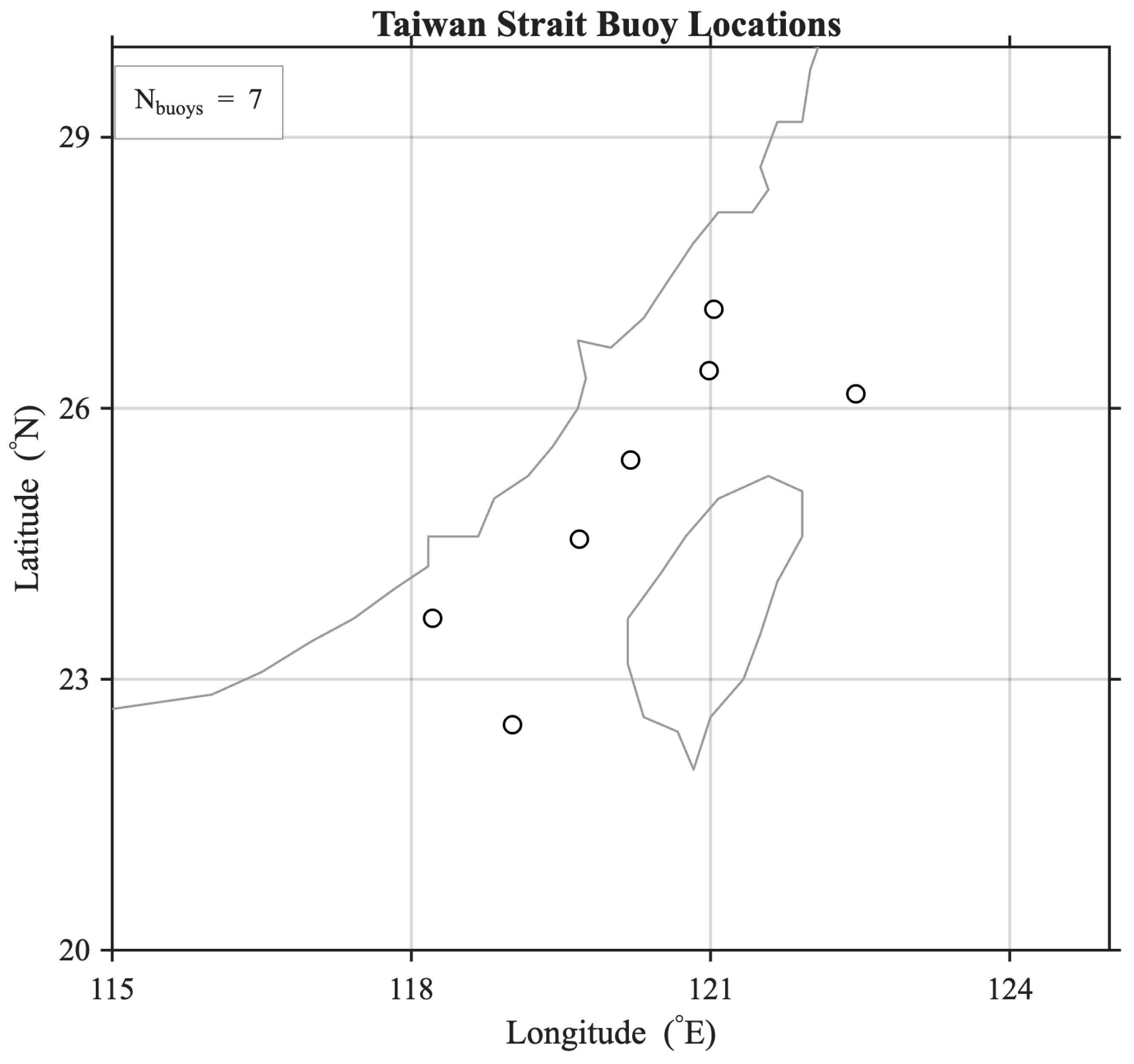
In previous validation studies of satellite altimeter SWH products, buoy-measured SWH is typically regarded as the ground truth and temporally and spatially collocated with satellite observations. In this study, observations from the National Data Buoy Center (NDBC) network collected between January 2022 and December 2023 were primarily used for satellite altimeter validation. NDBC buoys provide long-term, stable observations with rigorous calibration and quality-control procedures, ensuring consistency and reliability across platforms. These buoys are widely recognized as a benchmark reference in altimeter validation studies, and their well-characterized error statistics (typically <0.2 m for SWH) allow direct comparison with satellite products without introducing substantial additional uncertainty. In addition, we collected data from seven buoys deployed by the Fujian Marine Forecasts in the Taiwan Strait and adjacent waters. Previous studies have shown that these buoys have reliable data quality [17]. These observations cover the entire year of 2022, with sampling intervals of either 10 min or 1 h. The recorded parameters include SWH, wind speed, wind direction, air temperature, and atmospheric pressure. The locations of the NDBC buoys and the Taiwan Strait buoys are shown in Figure 1 and Figure 2, respectively. Quartly et al. showed that including collocations too close to the coast degrades altimeter–buoy statistics, underscoring the need for conservative coastal masks or distance-to-shore thresholds in validation studies [18]. Altimeter–buoy validation was restricted to buoys at least 50 km offshore, a common threshold to avoid coastal contamination of the altimeter footprint. Coastal contamination primarily arises from waveform distortion over mixed land/sea footprints and rapidly varying bathymetry or breaking waves; a conservative 50 km distance-to-coast mask has been shown to materially reduce such effects while retaining sufficient samples [18].

2.2. Altimeter Data

We used the HY-2B GDR data provided by the National Satellite Ocean Application Service. These calibrated products are derived using precise orbit ephemeris (POE) data and waveform retracking techniques, and include SWH, sea surface wind speed, and the necessary correction parameters for sea surface height retrieval. The dataset spans from 1 January 2022 to 31 December 2023 and is provided in NetCDF format. For this study, we used the SWH measured in the Ku-band (swh_ku) as the primary research variable. The HY-2B GDR products are publicly released through the NSOAS Ocean Satellite Data Distribution System (https://osdds.nsoas.org.cn, (accessed on 12 October 2025)), which currently provides access to registered users within China.

2.3. Model Data

The CMEMS Global Ocean Waves Reanalysis product (GLOBAL_MULTIYEAR_WAV_001_032) provides multi-year, high-quality wave fields derived from numerical wave modeling and data assimilation. It features a spatial resolution of 0.2° × 0.2° and a temporal resolution of 3 h, offering global coverage. Wave parameters are interpolated using the optimal interpolation method of the native grid model [19]. In this study, we used VHM0 from the CMEMS Global Wave Reanalysis for the period 1 January 2022 to 31 December 2023. These model SWH fields were not only collocated with buoy observations for triple-collocation analysis but also served as the predictor variable in the subsequent scaling experiments: the bias correction, ordinary least-squares (OLS) linear regression scaling, and machine-learning residual modeling all take the collocated VHM0 values as the reference ’model SWH’ input when estimating corrections to buoy SWH. The dataset is publicly available from the Copernicus Marine Environment Monitoring Service at https://data.marine.copernicus.eu/, (accessed on 12 October 2025).

2.4. Collocation, QC, and Interpolation

In previous studies, some authors adopted a “multi-point averaging” strategy for altimeter–buoy collocation, where all altimeter observations within 50 km of the buoy along a single pass were averaged if the number of points exceeded seven (i.e., at least eight valid measurements). Considering the ∼7 km along-track sampling of the HY-2B altimeter at 1 Hz, a simple geometric calculation shows that at least eight points can only be obtained when the track passes within approximately 44 km of the buoy. This approach reduces random noise by averaging multiple observations, yielding a smoother and more representative estimate of the sea state. However, it also discards many potential collocations, as a large fraction of passes provide only 1–3 valid points within 50 km. Moreover, averaging may suppress high-frequency variability, including extreme waves and localized anomalies. For this reason, the present study employs the nearest-point collocation method, which has also been adopted in previous works [4,5,10,18,20]. Campos combined altimeter records from the Australian Ocean Data Network (AODN) with NDBC buoy data to analyze the space–time variability of SWH (SWH) and 10 m wind ( U 10 ), systematically testing spatial (10, 25, 50, 100, 200 km) and temporal windows for matching. A 30 min time window paired with a 50 km radius provided the best compromise between accuracy and sample size, yielding reliable altimeter–buoy comparisons while retaining sufficient collocations [20], thereby retaining all available matches within the 50 km and 30 min thresholds.However, the altimeter dataset from the Australian Ocean Data Network (AODN) used in the study by Campos includes measurements from GEOSAT, ERS-1, TOPEX, ERS-2, GFO, Jason-1, ENVISAT, Jason-2, CRYOSAT-2, HY-2A, SARAL, and Jason-3, and does not specifically investigate the HY-2 series altimeters. In the primary analysis we adopt a collocation threshold of 30 min and 50 km to ensure comparability with previous studies and sufficient sample size. To quantify the sensitivity to the spatial window and its effect on representativeness error, we perform a robustness analysis using 25, 50, 75 and 100 km thresholds and report sample counts and validation metrics (RMSE, bias, standard deviation and correlation) for each case. The temporal matching window was fixed at ±30 min, following Campos et al. [20] and Quartly et al. [18], which demonstrated that this tolerance provides an optimal balance between accuracy and sample size in altimeter–buoy validation.
To ensure the reliability of collocated HY-2B and reference observations, a series of quality control (QC) filters were applied prior to analysis. Measurements flagged for land contamination, rain, or tracker failure in the HY-2B GDR were first removed. Observations acquired at off-nadir angles exceeding 0 . 3 ° were excluded to avoid geometric mispointing and waveform distortion. To minimize coastal contamination, only matchups located farther than 50 km from the nearest coastline were retained. For reference buoy and model datasets, range and temporal consistency checks were applied to remove physically unrealistic or spurious values. Finally, statistical outliers were filtered using the interquartile range (IQR) criterion, as described below. After all QC steps, approximately 90% of the original collocations were retained for subsequent validation and calibration. The resulting dataset ensures that only geometrically and physically consistent observations are used in the following analyses.
In this study, VHM0 from the numerical model was interpolated onto the locations and observation times of the buoys using three-dimensional linear interpolation. First, the model coordinate axes—longitude, latitude, and time—were preprocessed to ensure strict monotonicity and consistency: longitude was converted to the range [ 0 , 360 ) , the time variable (seconds since 1 January 1970 ) was converted to MATLAB R2025a serial days, and each axis was sorted in ascending order with duplicates removed, while the VHM0 array was synchronously reordered. Interpolation was then performed with MATLAB’s interpn in vector-axis mode, which directly accepts one-dimensional longitude, latitude, and time vectors. Linear interpolation was applied in all three dimensions, and points outside the model domain were assigned NaN to avoid artificial extrapolation. During interpolation of CMEMS model fields to buoy observation points, approximately 3% of potential collocations fell outside the model’s spatiotemporal domain and were assigned NaN values; these were excluded to prevent artificial extrapolation. The interquartile range (IQR) filter was applied with a Tukey threshold of k = 1.5 , i.e., matchups with residuals outside Q 1 1.5 IQR , Q 3 + 1.5 IQR were discarded, where Q 1 and Q 3 denote the first and third quartiles of the altimeter–buoy residuals and IQR = Q 3 Q 1 .
For routine Cal/Val practice, the validated configuration can thus be summarized as a three-step workflow: applying standard QC filters (land/rain/tracker flags, off-nadir > 0 . 3 ° , distance-to-coast > 50  km, range checks, and IQR outlier removal), collocating with a ± 30  min time window and 25–50 km radius, and diagnosing performance through sea-state-binned RMSE/STD and, where appropriate, OLS or residual-ML scaling in coastal regimes.

2.5. Calibration Schemes: Bias, OLS, and ML Residual Correction

To reconcile model-derived SWH with buoy observations and to provide a consistent reference for altimeter validation, three complementary scaling approaches are applied.

2.5.1. Bias Correction

The simplest adjustment removes the mean additive difference between model and buoy SWH:
H cal ( bias ) = H mod + Δ b ,
where
Δ b = 1 N i = 1 N H buoy , i H mod , i .
This method effectively corrects systematic offsets but does not address scale-dependent (multiplicative) errors.

2.5.2. OLS Linear Regression Scaling

To account for both additive and multiplicative discrepancies, an OLS slope–intercept regression is fitted:
H cal ( OLS ) = α H mod + β ,
where α and β are estimated by minimizing the residual sum of squares between buoy and model SWH. This linear mapping is flexible and transparent, although it assumes a strictly linear relationship.

2.5.3. Machine-Learning Residual Correction

To capture nonlinear dependencies and environmental influences, we adopt an ensemble regression framework. The residual
R = H buoy H mod
is modeled as a function of physical predictors (model SWH, wind speed, wind direction, and buoy ID) using a bagged regression-tree ensemble implemented in MATLAB (fitrensemble):
H cal ( ML ) = H mod + R ^ .
In this framework, the buoy ID was not included as an input feature. Instead, it was used solely as a grouping variable for K-fold cross-validation, ensuring that all observations from a given buoy remain entirely within either the training or validation set and thus preventing site-specific information leakage. This strategy effectively corresponds to a leave-one-buoy-out validation configuration, providing a robust estimate of the model’s ability to generalize to unseen buoys. We used an ensemble of 120 trees with a minimum leaf size of five, with hyperparameters set a priori based on exploratory trials to balance bias and variance. Model performance was evaluated using buoy-wise grouped K-fold cross-validation, confirming stable performance and no overfitting to specific buoy sites.
Together, these three methods span increasing levels of complexity: bias correction provides a quick adjustment, OLS regression scaling offers a statistically grounded linear solution, and ML residual correction captures more complex, context-dependent errors.

3. Results and Discussion

3.1. Threshold Sensitivity

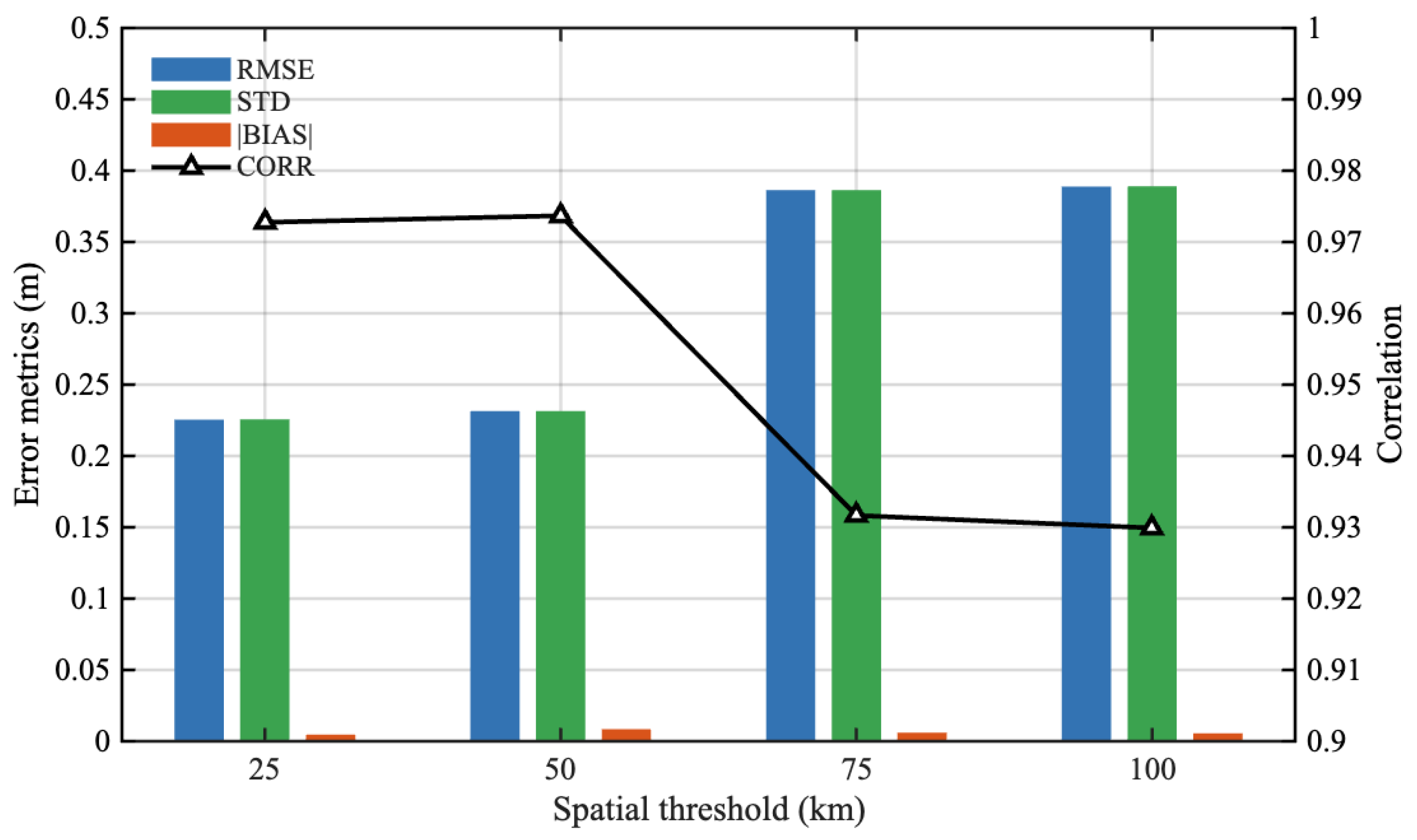
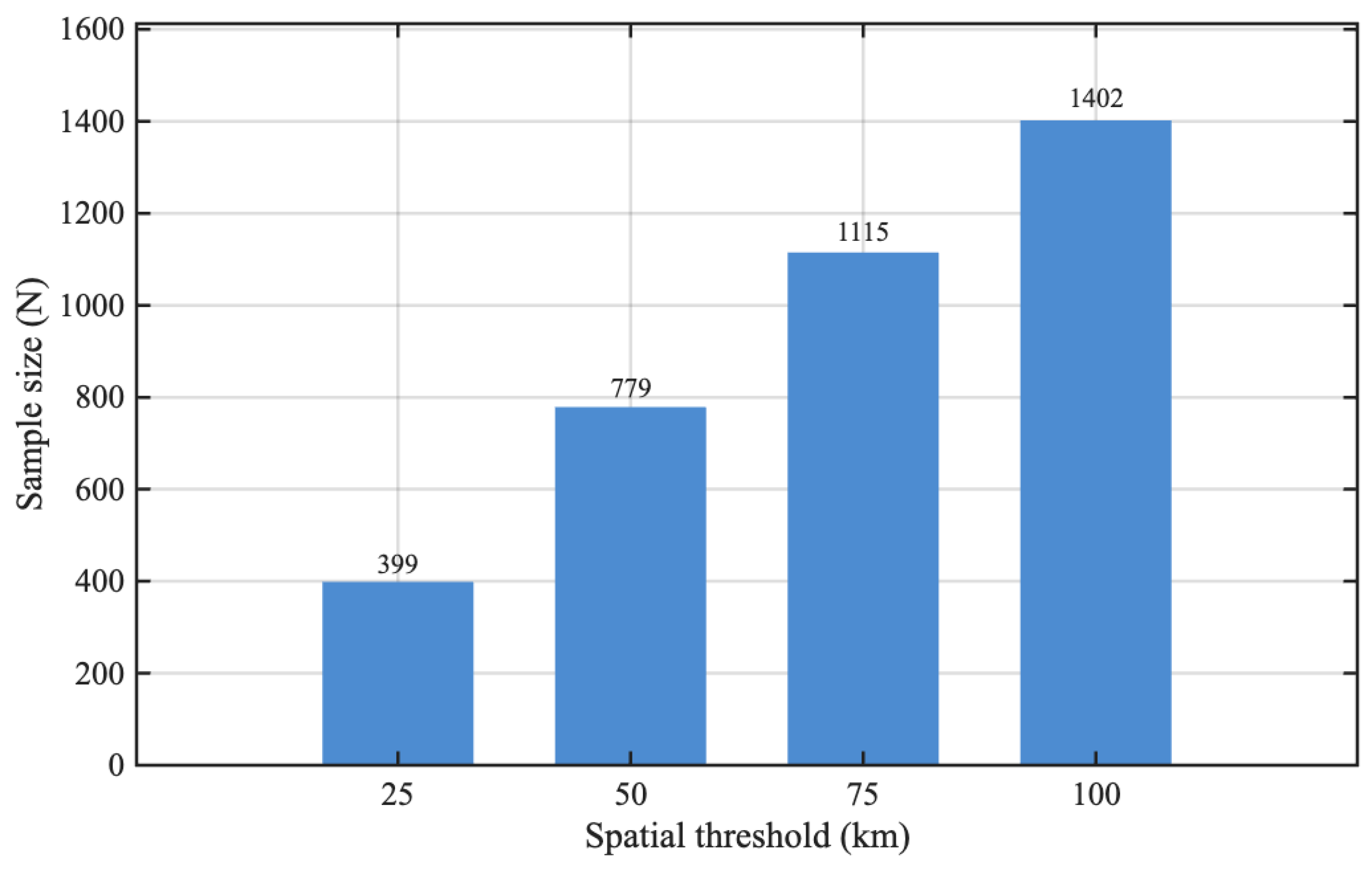
To quantify the sensitivity to the spatial window and assess how different collocation thresholds influence validation quality and representativeness error, we evaluated error statistics under four distance limits (25, 50, 75, and 100 km) . The results are illustrated in Figure 3. Figure 3 and Figure 4 summarize the sensitivity of the altimeter–NDBC buoy collocation results to different spatial-matching thresholds. As the collocation radius increases from 25 km to 100 km, the sample size grows 3 times (from 399 to 1402; Figure 4), providing more coincident measurements but simultaneously degrading the agreement between the altimeter and buoy SWH observations. Figure 3 illustrates how the validation statistics of HY-2B altimeter SWH vary with the spatial collocation threshold. As the matching radius widens from 25 km to 100 km, the root mean square error (RMSE, blue bars) and the residual standard deviation (STD, green bars) show a pronounced increase, rising from about 0.23 m at the tightest threshold to nearly 0.40 m at 75–100 km. In contrast, the absolute mean bias (orange bars) remains very small (<0.02 m) across all thresholds, confirming that the error growth is dominated by random scatter rather than a systematic offset. The correlation coefficient (black line with triangles, right axis) stays high (≈0.98) for 25–50 km but declines steadily to ≈0.93 once the threshold exceeds 75 km, reflecting increasing representativeness errors when spatial matching is relaxed. Table 1 summarizes quantitative descriptions of the sensitivity of matching statistics to spatial window selection. These results highlight the expected trade off: a narrow collocation window yields the most accurate agreement between altimeter and buoy SWH but limits the number of coincident observations, whereas broader windows enlarge the sample size at the cost of degraded precision and correlation.

3.2. Overall and Sea-State-Binned Results

We first present overall collocation results under four spatial thresholds (25/50/75/100 km; ±30 min).
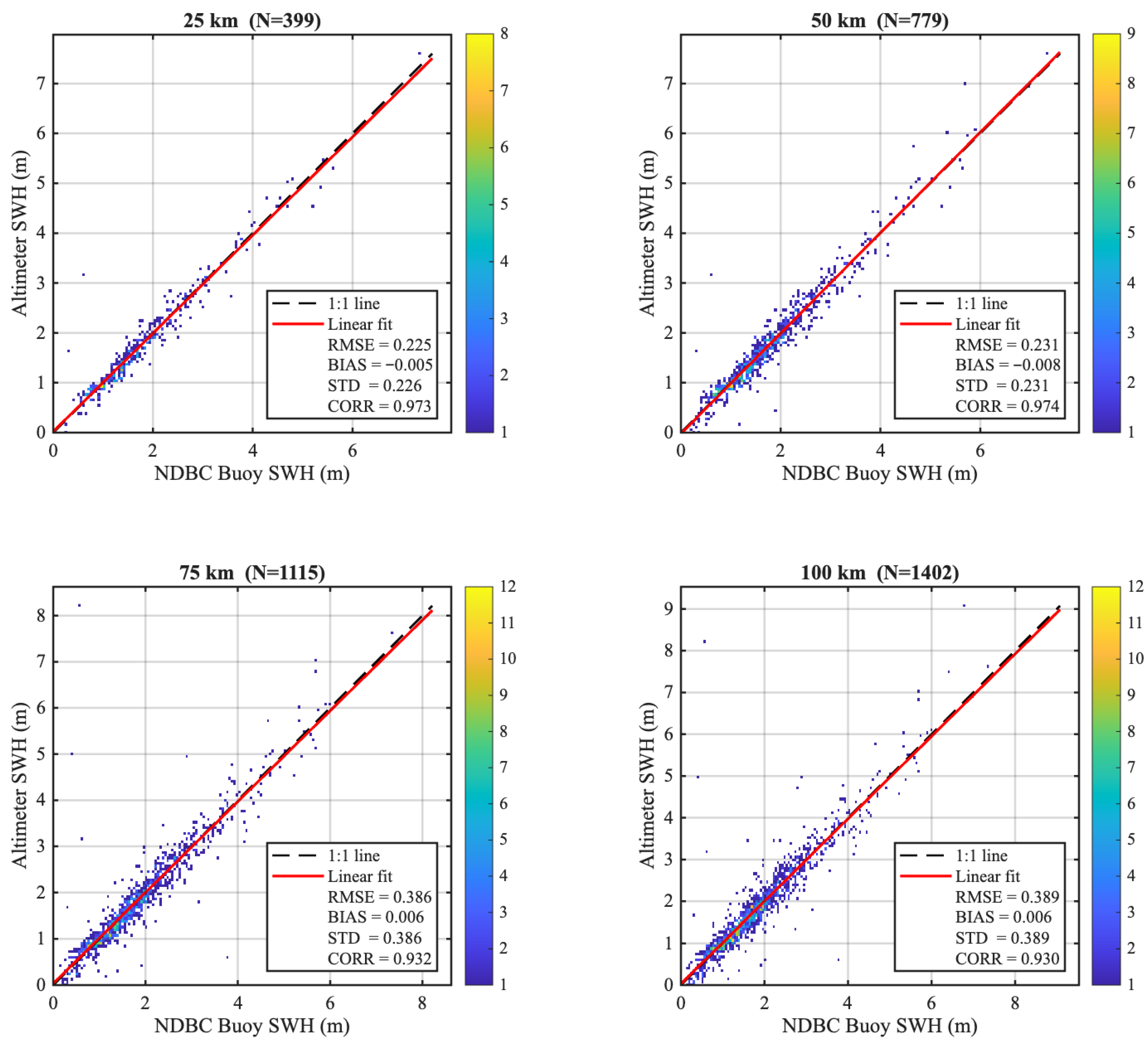
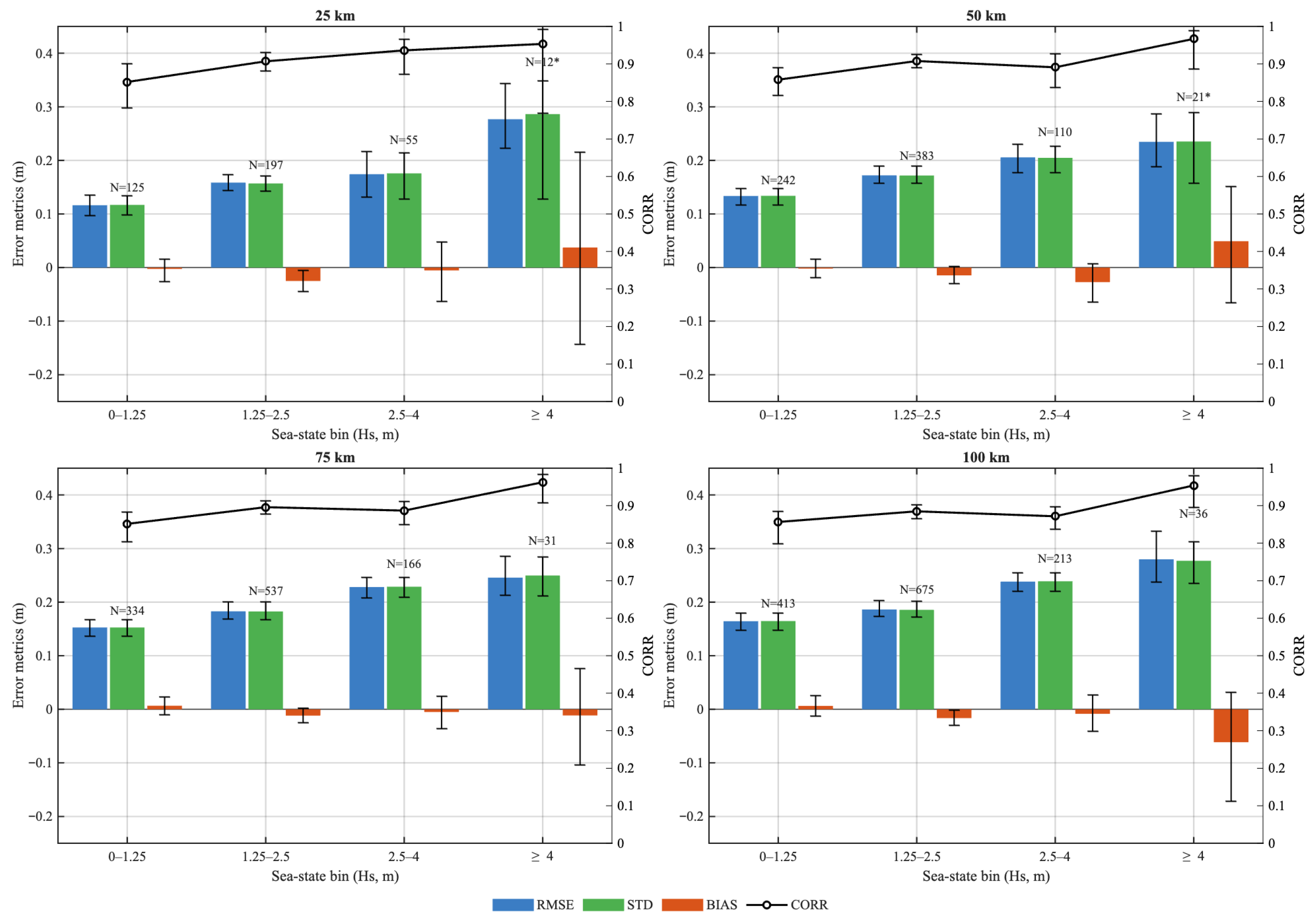
Figure 5 presents density scatterplots comparing HY-2B altimeter SWH with NDBC buoy observations under four spatial collocation thresholds: 25, 50, 75, and 100 km. Figure 6 summarizes the error statistics of HY-2B altimeter SWH against NDBC buoy observations, stratified by World Meteorological Organization (WMO) sea state classes and four spatial collocation thresholds (25, 50, 75, and 100 km). Across all thresholds, the root mean square error (RMSE) and residual standard deviation (STD) systematically increase with sea state, rising from roughly 0.15–0.20 m in calm to slight conditions (0–1.25 m) to more than 0.25–0.30 m in rough seas (SWH ≥ 4 m). The correlation coefficient (CORR) remains high (>0.85) even in the highest sea state bin, demonstrating that the altimeter maintains strong fidelity under energetic wave conditions despite the increased scatter. Mean bias remains negligible ( | BIAS | < 0.05 m) across most bins and thresholds, with slightly larger negative bias appearing in the ≥4 m category at the widest spatial windows, likely reflecting sampling differences when extreme events are sparsely observed. Comparing panels reveals that enlarging the collocation radius increases sample size but also amplifies random error: the 25–50 km thresholds yield the lowest RMSE/STD and the most stable correlation, whereas 75–100 km windows show larger spread and slightly reduced CORR. These results highlight that both sea state intensity and spatial representativeness strongly influence validation accuracy, and they support the adoption of a tighter 25–50 km threshold for the most reliable HY-2B SWH calibration. For higher sea-state bins (SWH > 3–4 m), the number of collocated samples decreases because such energetic conditions are relatively rare within the study region. Although the reduced sample size increases statistical uncertainty, the monotonic increase of RMSE and STD with sea state remains consistent, confirming the robustness of the result. The 95% confidence intervals for RMSE and correlation coefficients are narrow (within ±0.02) and are omitted from the plots for clarity.
Two generic patterns emerge: (i) increasing the spatial threshold enlarges the sample size but typically degrades RMSE/STD because of enhanced representativeness mismatch; (ii) sea state matters—bias and scatter—often grow in higher-SWH bins. To address these effects, we therefore incorporate both buoy and model predictors when applying the scaling approaches (bias correction, OLS linear regression scaling, and machine-learning residual correction) and revisit these diagnostics to quantify the potential gains, particularly in bins where discrepancies are most pronounced.

3.3. Scaling Performance: NDBC Versus Taiwan Strait Buoys

To rigorously evaluate the proposed validation–scaling framework, we adopted two complementary buoy datasets: (i) the U.S. National Data Buoy Center (NDBC) network and (ii) seven domestic buoys deployed in the Taiwan Strait. Both datasets are from 2022. The NDBC array provides long-term, well-calibrated, open-ocean observations with documented random errors typically below 0.2 m. In contrast, the Taiwan Strait buoys operate in a semi-enclosed coastal regime and, although subject to standard quality control, are potentially more affected by representativeness errors (e.g., coastal bathymetry, shorter fetch, local wind variability) and by limitations in sensor calibration and maintenance. This strategy enables us to (a) establish an international benchmark for HY-2B SWH accuracy using a globally recognized reference (NDBC) and (b) test the practical benefits of bias, regression, and machine-learning (ML) residual scaling in a more challenging, regionally specific environment.
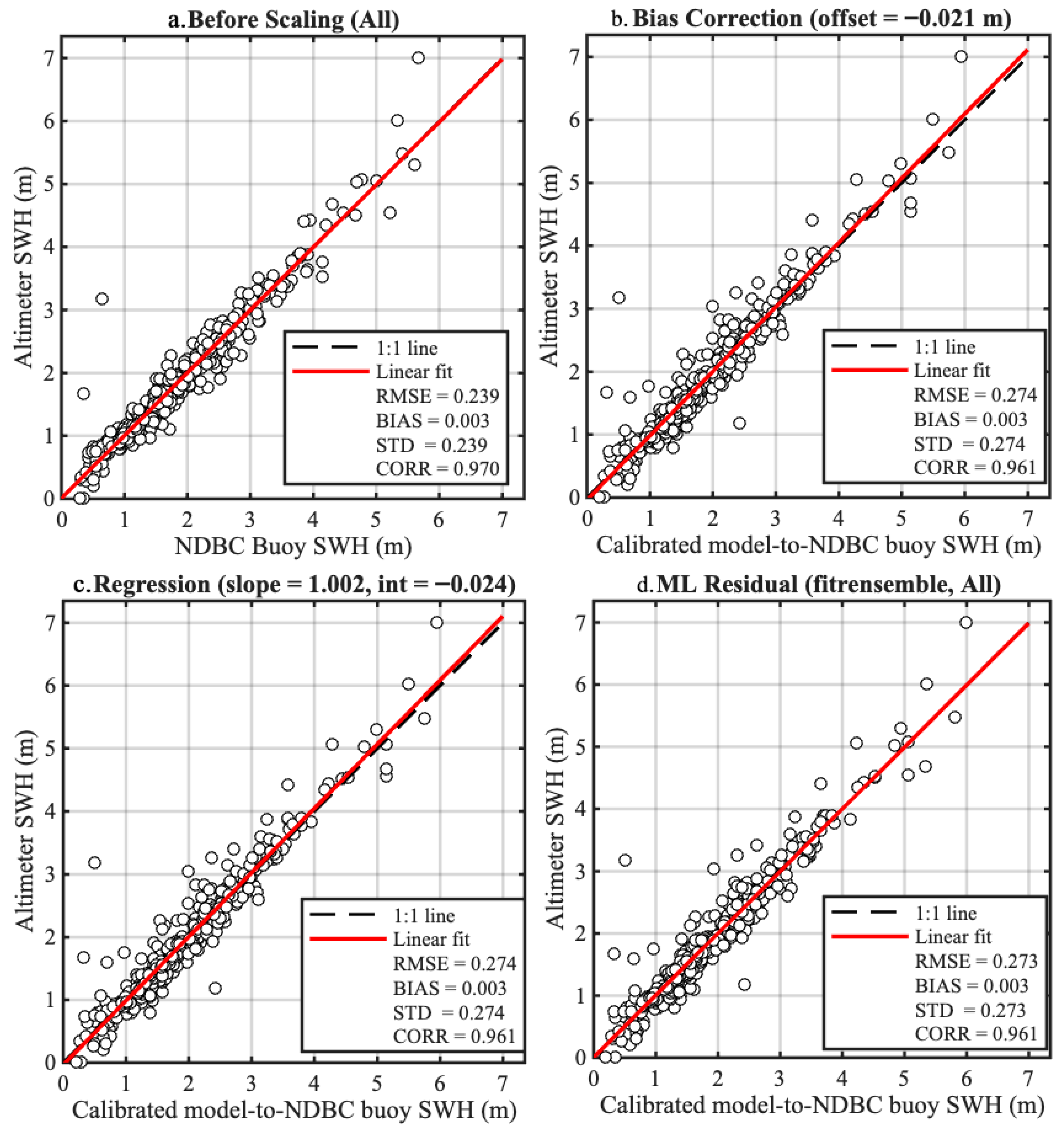
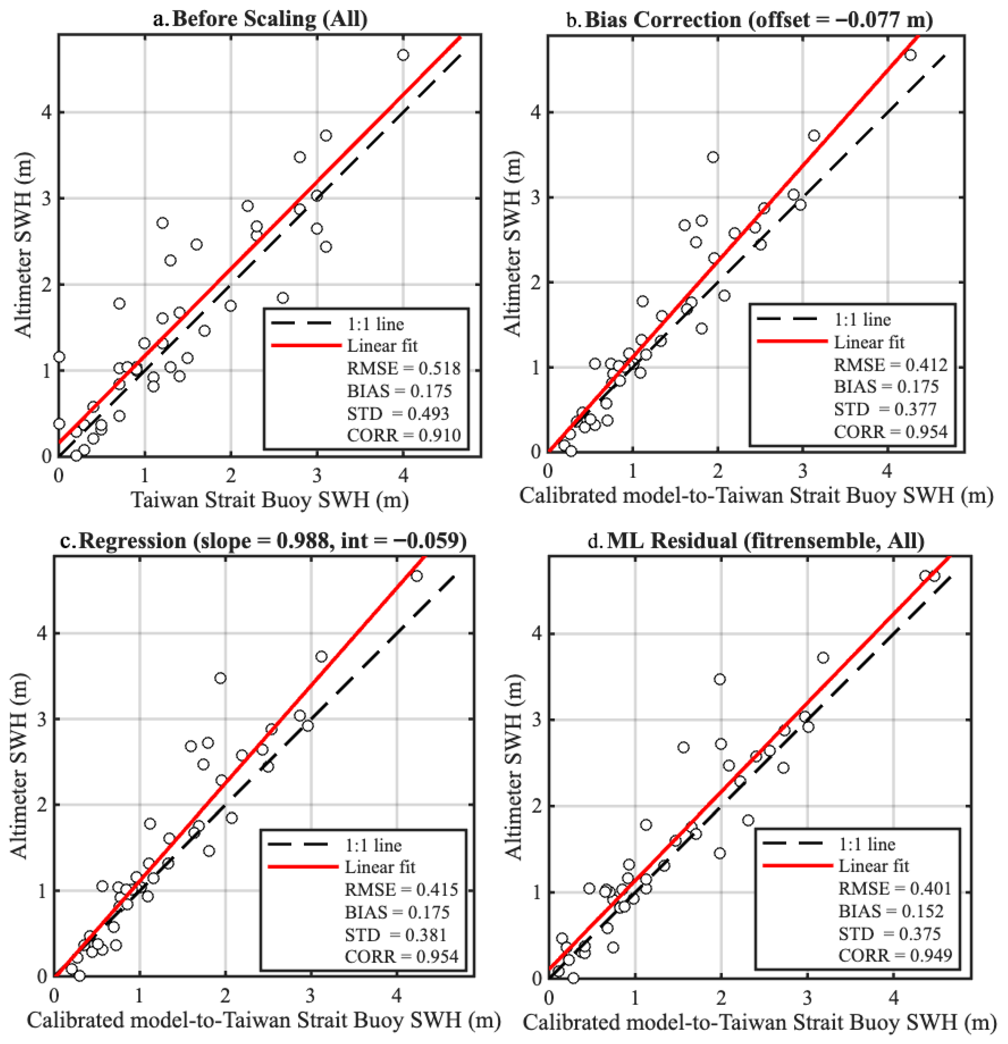
Figure 7 shows the scaling experiments for the NDBC matchups. Before scaling, HY-2B SWH already agrees extremely well with NDBC SWH, exhibiting RMSE = 0.239 m, negligible mean bias (0.003 m), and a correlation coefficient of 0.970. Applying constant-bias correction, ordinary least squares (OLS) regression, or ML residual modeling does not improve these metrics; in fact, RMSE and STD slightly increase (to ∼0.27 m) and correlation drops marginally (∼0.961). These results confirm that for high-quality, well-calibrated NDBC buoys, additional scaling provides no benefit and may introduce minor noise. Figure 8 contrasts the results for the Taiwan Strait buoys. Here, the unscaled comparison shows a larger RMSE of 0.518 m, a positive bias of 0.175 m, and a lower correlation of 0.910. All three scaling approaches markedly improve the fit: constant-bias and regression reduce RMSE to ≈0.41 m and raise the correlation to ≈0.95, while the ML residual model achieves the best overall performance (RMSE = 0.401 m, STD = 0.375 m). These gains reflect the combined effects of more complex coastal dynamics and slightly lower instrumental accuracy, where statistical or machine-learning corrections are demonstrably beneficial. In particular, after bias correction and scaling, the uncertainty of the Taiwan Strait buoy matchups expressed as the random error standard deviation was reduced by about 20% relative to the uncorrected case.
The machine-learning residual correction trained using the Taiwan Strait buoy dataset is region-specific, representing marginal-sea conditions roughly within 23–26°N and 117–121°E. Its parameters are not directly transferable to other regions, where sea-state characteristics and coastline geometry differ.

3.4. Extended Triple Collocation Results

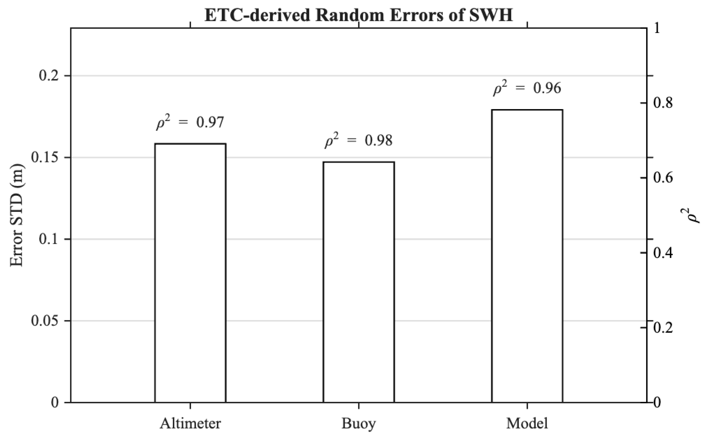
Originally developed for scatterometer wind validation, triple collocation provides unbiased random-error variances for three independent data sources without assuming a known truth [21,22,23,24]. The CMEMS wave reanalysis assimilates SWH observations from multiple altimeter missions, including ERS-1, TOPEX/Poseidon, ERS-2, GFO, Jason-2/3, Envisat, Saral, CryoSat-2, and Sentinel. Although some of these missions overlap temporally with HY-2B, the CMEMS data assimilation system employs a short assimilation window (typically within ±6 h) and spatial averaging at the model grid scale. These constraints minimize temporal and spatial correlations with non-assimilated sensors. Because neither HY-2B altimeter data nor NDBC buoy observations are included in the assimilation stream, any residual cross-dependence is expected to be negligible, and the three datasets can be reasonably regarded as mutually independent for the present ETC analysis [19]. McColl et al. further introduced an extended formulation that also retrieves the correlation coefficient of each system with the unknown target variable [25]. ETC calculates the covariance matrix of collocated triplets and uses analytical expressions to derive both the error variance and the correlation coefficient for each data source, under the assumptions that their errors are uncorrelated and have zero mean. This framework allows a consistent, sensor-independent assessment of measurement noise and intercomparison of the three systems, enabling a robust evaluation of satellite altimeter SWH accuracy relative to buoy and model references [25]. Figure 9 and Table 2 summarize the Extended Triple Collocation (ETC) estimates for collocated HY-2B SWH, NDBC buoy SWH, and the VHM0 during 2022–2023. Under the standard ETC assumptions (linearity of the signal–error model and mutually uncorrelated sensor errors), the method separates instrument/model-specific random errors without declaring any source as the truth. The buoy exhibits the smallest random error (Error STD = 0.147 m), followed by the altimeter ( 0.158 m), whereas the model shows the largest error ( 0.179 m). The ETC correlations are uniformly high ( ρ > 0.98 , ρ 2 0.96 0.98 ), indicating that all three records capture a common geophysical signal with excellent coherence. The ordering of errors is physically consistent: in situ buoys minimize representativeness mismatch; the altimeter contains additional footprint-scale variability and retracking noise; and the model inherits numerical and assimilation errors as well as representativeness differences relative to point measurements. The differences are nonetheless modest (on the order of 0.01–0.03 m), and the high ρ 2 values annotated in Figure 9 corroborate the strong agreement among the three systems. These results provide an internally consistent benchmark and an independent cross-check of the scaling findings above, confirming that HY-2B SWH is closely aligned with buoy observations while the CMEMS product retains slightly larger random variance at matchup scales considered.
Future studies may additionally remove triplets located close in space or time to known assimilated overpasses to further minimize any residual cross-dependence.

3.5. Implications and Key Findings

The contrasting outcomes underscore a central conclusion:
  • For NDBC buoys with well-characterized uncertainties, buoy SWH requires no additional scaling. The satellite and buoy observations are already statistically consistent within their respective noise levels.
  • For regional coastal buoys of good but less rigorously calibrated quality (Taiwan Strait), systematic and random errors are larger; here, our unified scaling framework—particularly the ML residual correction—provides a substantial reduction in random scatter and bias.
This evidence supports a data-quality-driven strategy for altimeter calibration: scaling is not universally necessary but should be selectively applied when the in situ reference is less stable or represents more heterogeneous coastal conditions. Such guidance is valuable for operational agencies planning validation campaigns in regions where buoy quality and environmental variability differ from the NDBC standard. In practice, bias correction is useful for quick calibration, OLS linear regression scaling provides a more comprehensive linear adjustment, while machine learning residual modeling has the greatest potential to minimize uncertainty when sufficient collocated data are available. Nevertheless, machine learning methods should be carefully validated (e.g., through cross-validation or buoy-wise grouped testing) to ensure robust generalization across different buoy sites and environmental regimes.

4. Conclusions

We presented a unified workflow for HY-2B SWH validation that combines nearest-point collocation, sea-state-binned diagnostics, three complementary scaling schemes, and ETC-based uncertainty assessment. The main findings are:
  • Collocation sensitivity. Using NDBC buoys as a reference, spatial thresholds exert first-order control on performance. Narrow windows (25–50 km with 30 min) yield the lowest RMSE/STD and the highest correlations; broader windows increase sample size but degrade precision due to representativeness errors, especially at high sea state.
  • Sea-state dependence. Across thresholds, RMSE/STD increase with SWH while mean biases remain small, indicating that error growth is dominated by random scatter rather than systematic offsets. Reporting sea-state-binned metrics is therefore recommended for operational validation.
  • Data-quality-driven scaling. For high-quality NDBC matchups, HY-2B and buoy SWH are already consistent (e.g., RMSE ≈ 0.24 m), and bias/OLS/ML adjustments do not improve performance and may slightly increase scatter. In contrast, for Taiwan Strait buoys in a more heterogeneous coastal regime, all three schemes reduce errors, with the machine-learning residual correction providing the largest improvement (e.g., RMSE ≈ 0.40−0.41 m, correlation ≈ 0.95).
  • Sensor-independent uncertainty. ETC applied to HY-2B, NDBC, and CMEMS over 2022–2023 indicates random error standard deviations of 0.158, 0.147, and 0.179 m, respectively, with consistently high ρ 2 (≈0.96–0.98), confirming strong coherence among the three systems at matchup scales.
Practical guidance. For HY-2B SWH validation, we recommend a 30 min/25–50 km window, explicit QC, and selective use of OLS or residual machine-learning scaling where buoy quality and coastal heterogeneity warrant correction. Future work will extend the analysis to additional HY-2 missions and regions, explore adaptive spatiotemporal windows and uncertainty-aware scaling, and assess benefits from multi-sensor wave products.

Author Contributions

Conceptualization, S.Y. and H.P.; methodology, S.Y. and H.P.; software, S.Y.; validation, S.Y., H.P. and L.Z.; formal analysis, S.Y.; investigation, S.Y.; resources, H.P.; data curation, S.Y.; writing—original draft, S.Y.; writing—review and editing, H.P., L.Z., W.Z., Q.S., B.M. and Y.Z.; visualization, S.Y.; supervision, H.P.; project administration, H.P.; funding acquisition, H.P. All authors have read and agreed to the published version of the manuscript.

Funding

This research was funded by the National Key Research and Development Program of China, grant number 2023YFB3905802.

Institutional Review Board Statement

Not applicable.

Informed Consent Statement

Not applicable.

Data Availability Statement

HY-2B GDR data: https://osdds.nsoas.org.cn (accessed on 12 October 2025); NDBC buoy data: https://www.ndbc.noaa.gov (accessed on 12 October 2025); CMEMS wave reanalysis (GLOBAL_MULTI-YEAR_WAV_001_032): https://data.marine.copernicus.eu (accessed on 12 October 2025).

Acknowledgments

The authors express their sincere gratitude to the Fujian Marine Forecasts for providing the Taiwan Strait buoy data and to the National Data Buoy Center (NDBC) for supplying the NDBC buoy data. We also extend our appreciation to McColl et al. for making the Extended Triple Collocation (ETC) analysis method available.

Conflicts of Interest

The authors declare no conflict of interest.

References

  1. Ribal, A.; Young, I.R. 33 Years of Globally Calibrated Wave Height and Wind Speed Data Based on Altimeter Observations. Sci. Data 2019, 6, 77. [Google Scholar] [CrossRef] [PubMed]
  2. Young, I.R.; Ribal, A. Multiplatform Evaluation of Global Trends in Wind Speed and Wave Height. Science 2019, 364, 548–552. [Google Scholar] [CrossRef] [PubMed]
  3. Liu, Q.; Babanin, A.V.; Guan, C.; Zieger, S.; Sun, J.; Jia, Y. Calibration and Validation of HY-2 Altimeter Wave Height. J. Atmos. Ocean. Technol. 2016, 33, 919–936. [Google Scholar] [CrossRef]
  4. Qin, D.; Jia, Y.; Lin, M.; Liu, S. Performance Evaluation of China’s First Ocean Dynamic Environment Satellite Constellation. Remote Sens. 2023, 15, 4780. [Google Scholar] [CrossRef]
  5. Li, X.; Xu, Y.; Liu, B.; Lin, W.; He, Y.; Liu, J. Validation and Calibration of Nadir SWH Products From CFOSAT and HY-2B with Satellites and In Situ Observations. J. Geophys. Res. Ocean. 2021, 126, e2020JC016689. [Google Scholar] [CrossRef]
  6. Yang, J.; Zhang, J.; Jia, Y.; Fan, C.; Cui, W. Validation of Sentinel-3A/3B and Jason-3 Altimeter Wind Speeds and Significant Wave Heights Using Buoy and ASCAT Data. Remote Sens. 2020, 12, 2079. [Google Scholar] [CrossRef]
  7. Yang, L.; Xu, Y.; Lin, M.; Ma, C.; Mertikas, S.P.; Hu, W.; Wang, Z.; Mu, B.; Zhou, X. Monitoring the Performance of HY-2B and Jason-2/3 Sea Surface Height via the China Altimetry Calibration Cooperation Plan. IEEE Trans. Geosci. Remote Sens. 2022, 60, 1002013. [Google Scholar] [CrossRef]
  8. Zieger, S.; Vinoth, J.; Young, I.R. Joint Calibration of Multiplatform Altimeter Measurements of Wind Speed and Wave Height over the Past 20 Years. J. Atmos. Ocean. Technol. 2009, 26, 2549–2564. [Google Scholar] [CrossRef]
  9. Queffeulou, P. Long-Term Validation of Wave Height Measurements from Altimeters. Mar. Geod. 2004, 27, 495–510. [Google Scholar] [CrossRef]
  10. Wang, J.; Aouf, L.; Jia, Y.; Zhang, Y. Validation and Calibration of Significant Wave Height and Wind Speed Retrievals from HY2B Altimeter Based on Deep Learning. Remote Sens. 2020, 12, 2858. [Google Scholar] [CrossRef]
  11. Zhang, R.; Qi, J.; Yan, Q.; Fan, C.; Yang, Y.; Zhang, J.; Wan, Y. Calibration of CFOSAT Off-Nadir SWIM SWH Product Based on CNN-LSTM Model. Earth Space Sci. 2024, 11, e2023EA003386. [Google Scholar] [CrossRef]
  12. Wang, J.; Yu, T.; Deng, F.; Ruan, Z.; Jia, Y. Acquisition of the Wide Swath Significant Wave Height from HY-2C through Deep Learning. Remote Sens. 2021, 13, 4425. [Google Scholar] [CrossRef]
  13. Yang, J.; Zhang, J. Validation of Sentinel-3A/3B Satellite Altimetry Wave Heights with Buoy and Jason-3 Data. Sensors 2019, 19, 2914. [Google Scholar] [CrossRef] [PubMed]
  14. Peng, H.; Lin, M. Calibration of HY-2A Satellite Significant Wave Heights with in Situ Observation. Acta Oceanol. Sin. 2016, 35, 79–83. [Google Scholar] [CrossRef]
  15. Jiang, M.; Xu, K.; Liu, Y. Calibration and Validation of Reprocessed HY-2A Altimeter Wave Height Measurements Using Data from Buoys, Jason-2, Cryosat-2, and SARAL/AltiKa. J. Atmos. Ocean. Technol. 2018, 35, 1331–1352. [Google Scholar] [CrossRef]
  16. Durrant, T.H.; Greenslade, D.J.M.; Simmonds, I. Validation of Jason-1 and Envisat Remotely Sensed Wave Heights. J. Atmos. Ocean. Technol. 2009, 26, 123–134. [Google Scholar] [CrossRef]
  17. Zhu, B.; Chen, J.; Xu, Y.; Zheng, Q.; Li, X. Validation of the CFOSAT Scatterometer Data with Buoy Observations and Tests of Operational Application to Extreme Weather Forecasts in Taiwan Strait. Earth Space Sci. 2022, 9, e2021EA001865. [Google Scholar] [CrossRef]
  18. Quartly, G.D.; Kurekin, A.A. Sensitivity of Altimeter Wave Height Assessment to Data Selection. Remote Sens. 2020, 12, 2608. [Google Scholar] [CrossRef]
  19. Copernicus Marine Environment Monitoring Service (CMEMS). Product User Manual for Global Ocean Wave Multi Year Product; GLOBAL_MULTIYEAR_WAV_001_032; Mercator Ocean International: Toulouse, France, 2024; Issue 1.4. [Google Scholar]
  20. Campos, R.M. Analysis of Spatial and Temporal Criteria for Altimeter Collocation of Significant Wave Height and Wind Speed Data in Deep Waters. Remote Sens. 2023, 15, 2203. [Google Scholar] [CrossRef]
  21. Janssen, P.A.E.M.; Abdalla, S.; Hersbach, H.; Bidlot, J.R. Error Estimation of Buoy, Satellite, and Model Wave Height Data. J. Atmos. Ocean. Technol. 2007, 24, 1665–1677. [Google Scholar] [CrossRef]
  22. Caires, S.; Sterl, A. Validation of Ocean Wind and Wave Data Using Triple Collocation. J. Geophys. Res. Ocean. 2003, 108, 2002JC001491. [Google Scholar] [CrossRef]
  23. Stoffelen, A. Toward the True Near-surface Wind Speed: Error Modeling and Calibration Using Triple Collocation. J. Geophys. Res. Ocean. 1998, 103, 7755–7766. [Google Scholar] [CrossRef]
  24. Vogelzang, J.; Stoffelen, A.; Verhoef, A.; Figa-Saldaña, J. On the Quality of High-Resolution Scatterometer Winds. J. Geophys. Res. 2011, 116, C10033. [Google Scholar] [CrossRef]
  25. McColl, K.A.; Vogelzang, J.; Konings, A.G.; Entekhabi, D.; Piles, M.; Stoffelen, A. Extended Triple Collocation: Estimating Errors and Correlation Coefficients with Respect to an Unknown Target. Geophys. Res. Lett. 2014, 41, 6229–6236. [Google Scholar] [CrossRef]
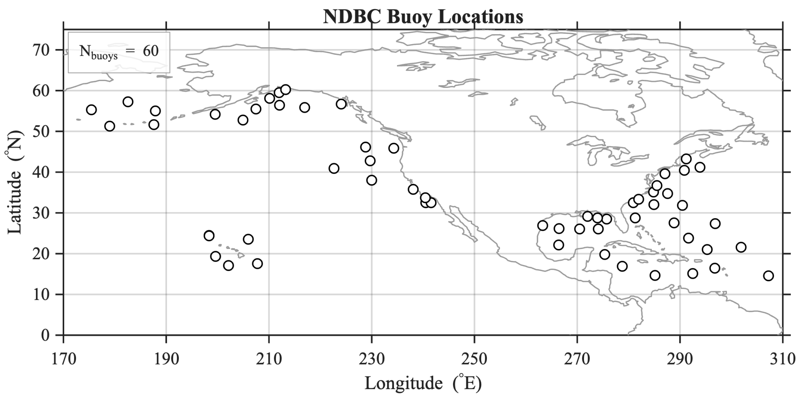
Figure 1. Geographical distribution of NDBC buoy locations.
Remotesensing 17 03829 g001
Figure 2. Locations of buoys in the Taiwan Strait.
Remotesensing 17 03829 g002
Figure 3. Error metrics (RMSE, STD, absolute bias) and correlation coefficient of altimeter–buoy SWH comparisons.
Remotesensing 17 03829 g003
Figure 4. Number of collocated altimeter–buoy pairs for each spatial matching threshold.
Remotesensing 17 03829 g004
Figure 5. Scatterplots of HY-2B altimeter versus NDBC buoy SWH for four spatial thresholds. Statistics include RMSE, mean bias, STD, and correlation coefficient (CORR).
Remotesensing 17 03829 g005
Figure 6. Error metrics binned by WMO sea-state classes for each spatial threshold. Bars denote RMSE (blue), STD (green), and mean bias (orange); black line with circles shows CORR. Asterisks (*) indicate sea-state bins with small sample size ( N < 30 ).
Remotesensing 17 03829 g006
Figure 7. Altimeter–NDBC buoy SWH comparison under four configurations: (a) before scaling; (b) Bias correction; (c) OLS linear regression scaling; and (d) machine-learning residual correction . The dashed line denotes the 1:1 reference and the red line the fitted relationship (N = 441).
Remotesensing 17 03829 g007
Figure 8. Same as Figure 7, but the buoy data is replaced with the Taiwan Strait buoy data (N = 44).
Remotesensing 17 03829 g008
Figure 9. Extended Triple Collocation (ETC) results.
Remotesensing 17 03829 g009
Table 1. Sample size (n) and error statistics of HY-2B vs. NDBC buoy SWH for different spatial collocation windows (±30 min).
 Window (km)Sample Size nRMSE (m)STD (m) 
253990.2250.226
507790.2310.231
7511150.3860.386
10014020.3890.389
Table 2. Extended Triple Collocation (ETC) results for HY-2B, NDBC buoys, and VHM0 over 2022–2023. Reported are the ETC random error standard deviation and correlation ( ρ ) with its square ( ρ 2 ).
SystemError STD (m) ρ ρ 2  
 Altimeter0.158390.987380.97491 
 Buoy0.147210.988420.97698 
 Model0.179220.982220.96476 
Disclaimer/Publisher’s Note: The statements, opinions and data contained in all publications are solely those of the individual author(s) and contributor(s) and not of MDPI and/or the editor(s). MDPI and/or the editor(s) disclaim responsibility for any injury to people or property resulting from any ideas, methods, instructions or products referred to in the content.