Article

Multi-Source Data Fusion and Ensemble Learning for Canopy Height Estimation: Application of PolInSAR-Derived Labels in Tropical Forests

1
Aerospace Information Research Institute, Chinese Academy of Sciences, Beijing 100094, China
2
University of Chinese Academy of Sciences, Beijing 100049, China
*
Author to whom correspondence should be addressed.
Remote Sens. 2025, 17(23), 3822; https://doi.org/10.3390/rs17233822
Submission received: 24 September 2025 / Revised: 23 October 2025 / Accepted: 20 November 2025 / Published: 26 November 2025
(This article belongs to the Special Issue SAR for Forest Mapping III)

Highlights

What are the main findings?
  • Airborne PolInSAR-derived continuous canopy height labels, enhanced with a hybrid baseline selection strategy, achieved higher inversion accuracy than conventional single-baseline approaches.
  • A dual-layer ensemble learning framework combining multi-source features (Landsat-8, GEDI, DEM, kNDVI) significantly improved canopy height prediction, reducing RMSE by 43.6% compared to existing global products.
What are the implications of the main findings?
  • PolInSAR-derived labels offer a reliable alternative to sparse or interpolated LiDAR data, enabling more accurate regional-scale canopy height mapping in complex tropical forests.
  • The proposed framework provides a transferable pathway for improving forest carbon stock estimation and ecosystem monitoring beyond current global products.

Abstract

Forest canopy height is essential for ecosystem process modeling and carbon stock assessment. However, most prediction approaches rely on sparse or interpolated LiDAR labels, leading to uncertainties in heterogeneous forests where laser footprints are limited or unevenly distributed. To address these issues, this study proposes a multi-source ensemble learning framework that uses airborne PolInSAR-derived continuous canopy height as training labels for accurate forest height prediction. The framework features two key innovations: (1) a hybrid baseline selection strategy (PROD+ECC) within the PolInSAR inversion, significantly improving the quality and stability of initial labels; (2) a dual-layer ensemble learning model that integrates machine learning and deep learning to interpret multi-source features (Landsat-8, GEDI, DEM, and kNDVI), enabling robust upscaling from local inversion to regional prediction. Independent validation in Gabon’s Akanda National Park achieved R2 = 0.748 and RMSE = 5.873 m, reducing RMSE by 43.6% compared with existing global products. This framework mitigates sparse supervision and extrapolation bias, providing a scalable paradigm for high-accuracy canopy height mapping in complex tropical forests and offering an effective alternative to LiDAR-based approaches for global carbon assessment.

Graphical Abstract

1. Introduction

Forests, as a core component of the global carbon cycle, fix carbon dioxide through photosynthesis and maintain the terrestrial carbon balance, making them key natural carbon sinks for mitigating global climate change [1,2]. Meanwhile, canopy height, as a fundamental parameter describing vertical structure, directly determines ecosystem energy exchange, water cycling, and biodiversity maintenance capacity [3,4]. Therefore, accurate inversion of forest canopy height is essential for ecological protection and sustainable development [5].
Traditional ground-based forest height measurements, although highly accurate, are costly, labor-intensive, and inefficient, limiting their applicability for large-scale dynamic monitoring [6]. The emergence of remote sensing has provided new solutions for canopy height estimation [7]. Early studies relied primarily on optical remote sensing data, such as Landsat-8 and Sentinel-2, which offer extensive spatial coverage and cost efficiency but suffer from cloud contamination and signal saturation in dense canopies, making it difficult to capture vertical structural information directly [8,9,10].
Spaceborne LiDAR missions such as GEDI and ICESat-2 provide precise vertical structural information; however, GEDI’s spatial coverage is limited to between 51.6°N and 51.6°S, sampling only about 4% of global land area during its mission [11]. ICESat-2, originally designed for polar ice sheet monitoring [12,13], is less optimized for forest applications [14]. The inherent sparsity of both datasets necessitates spatial interpolation or fusion with other remote sensing data to produce continuous canopy height maps [15,16], often introducing significant errors in complex forest environments [17,18,19,20,21,22,23].
Compared with spaceborne LiDAR, airborne LiDAR can capture denser, higher-resolution canopy height data [24,25], but its coverage is constrained by flight cost and logistics. In addition, topography [26] and the inability to penetrate ultra-dense canopies [27] can lead to “pits” or discontinuous patches comprising 15–20% of the mapped area [28]. As a result, interpolation and multi-source fusion are often required [29], which further increase uncertainty. For example, Potapov et al. [20] generated a global canopy height map using GEDI and Landsat data but found systematic underestimation of tall canopies and regional biases in tropical forests such as those in Gabon (RMSE = 10.419 m). Similarly, Lang et al. [21,22] produced a global canopy height product from GEDI and Sentinel-2 but reported reduced accuracy in complex tropical forests (RMSE = 11.057 m) and fragmented agroforestry landscapes. Liu et al. [29] also observed that spatial heterogeneity in LiDAR-derived labels introduced over 30% higher model errors in tropical than in temperate forests. These findings highlight the intrinsic limitations of sparse, discontinuous labels for canopy height prediction in heterogeneous tropical forests.
In contrast, microwave remote sensing [30], particularly Polarimetric Interferometric Synthetic Aperture Radar (PolInSAR) [31,32], combines the vertical sensitivity of InSAR with the scattering characterization of PolSAR, offering unique advantages for forest height retrieval [33,34,35]. Spaceborne PolInSAR processing techniques have matured considerably since their introduction [32,33,36,37,38,39,40], whereas airborne PolInSAR systems—less affected by temporal and spatial decorrelation [41,42]—offer higher resolution and improved accuracy in complex local forest environments [43]. Luo et al. [44], for instance, achieved high-precision canopy height inversion (RMSE = 5.38 m) in Gabonese mangrove forests using airborne multi-baseline PolInSAR data. Importantly, PolInSAR retrievals inherently produce continuous, high-resolution canopy height maps, eliminating the sparsity, interpolation bias, and label heterogeneity associated with LiDAR data.
However, two critical gaps remain in current PolInSAR-based studies. First, a single baseline selection strategy cannot adapt effectively to the full height gradient of tropical forests. Zhang et al. [45] found that the PROD method performs better in low (<10 m) and tall (>30 m) forests, whereas the ECC method is more suitable for intermediate heights (10–30 m) but less accurate in other ranges. Second, most existing studies focus on improving PolInSAR inversion algorithms themselves, without fully exploiting their potential as high-quality training labels for machine and deep learning models. Moreover, tropical forests—key global carbon sinks—exhibit high structural heterogeneity [44], frequent cloud cover, and strong spatial variability, where interpolation errors from sparse LiDAR labels can lead to biomass estimation biases of 20–30% [18]. Although PolInSAR enables continuous, all-weather observation, its extrapolation capability across larger regions (e.g., provincial scales) remains underdeveloped. Thus, integrating PolInSAR-derived continuous labels with multi-source remote sensing data to construct predictive models tailored to complex tropical forest environments is a pressing challenge.
To address these issues, this study proposes and validates a multi-source ensemble learning framework for canopy height estimation, replacing traditional sparse LiDAR samples with continuous canopy height maps derived from airborne PolInSAR. The main objectives and innovations are as follows:
(1)
Develop a high-quality PolInSAR labeling method by integrating a hybrid baseline selection strategy (PROD+ECC) within the advanced RVoG-VTDs model, improving inversion accuracy and stability in complex tropical forests;
(2)
Construct a dual-layer ensemble learning framework integrating machine learning and deep learning models, with an uncertainty-based dynamic weighting mechanism to exploit their complementary strengths in capturing heterogeneous and spatial contextual features;
(3)
Achieve robust upscaling from local inversion to regional prediction by training the model in Gabon’s Pongara National Park and validating it in the independent Akanda National Park, demonstrating the framework’s capacity to reduce extrapolation bias and enhance canopy height estimation accuracy.
In this study, we provide a novel paradigm for canopy height prediction in complex tropical forests by integrating PolInSAR-derived continuous labels with multi-source data and ensemble learning. The proposed framework expands the application potential of PolInSAR and offers a transferable pathway for regional forest mapping and carbon stock assessment.

2. Materials and Methods

2.1. Study Area

The study area is located in Gabon, on the west coast of Africa. Gabon is rich in natural resources, with a forest area of 20.4 million hectares, accounting for 76% of its national territory. Its exploitable timber volume is about 300 million cubic meters, ranking second in Africa, and it is known as the “Land of Forests.” The Congo Basin tropical rainforest is the second largest tropical rainforest in the world after the Amazon, and Gabon’s forests constitute an important part of this ecosystem. Meanwhile, with a forest cover exceeding 85%, Gabon’s forest ecosystems are both ecologically representative and structurally intact, making the country a key region for tropical forest conservation and carbon cycle research [6].
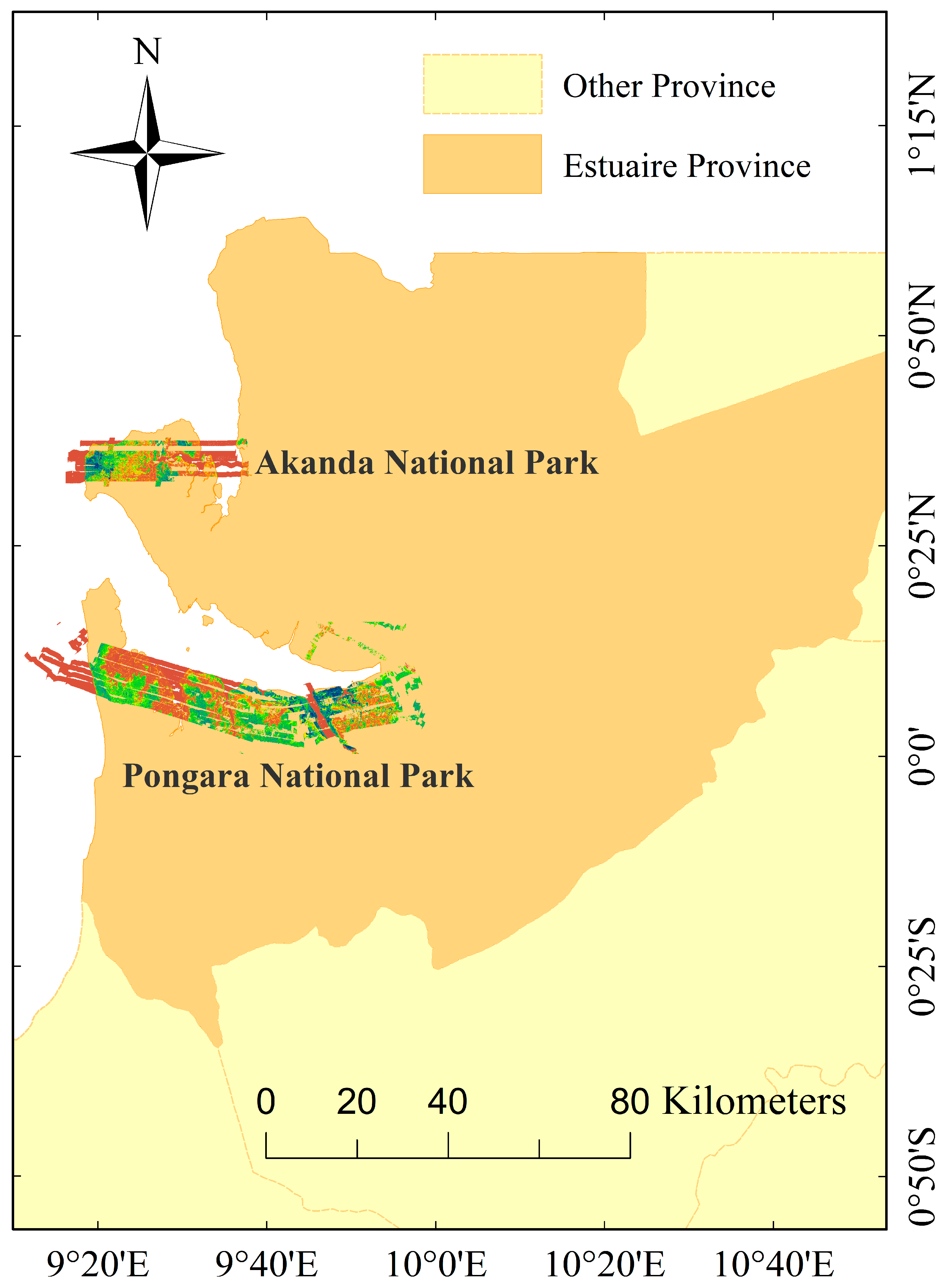
The data used in this study were collected from two national parks—Pongara and Akanda—both located in the Estuaire Province near the capital city Libreville (Figure 1). These two parks were among the core observation sites of NASA’s AfriSAR campaign (2016) [46,47], which provides comprehensive, co-registered multi-source datasets with standardized data processing protocols [48,49]. This ensures data accessibility, methodological reproducibility, and facilitates algorithmic development and optimization for forest structure studies.
Ecologically, the two experimental sites share similar forest structures and are highly representative of tropical coastal forest systems. Pongara National Park (9°10′–10°10′E, 0°0.3′S–0°15′N) is dominated by coastal mangrove forests with a relatively flat terrain but highly heterogeneous forest structures. The average canopy height is about 16 m, with localized maxima reaching up to 65 m due to the intermixing of tropical rainforest vegetation [44]. This structural variability introduces strong stochasticity, providing an ideal testing ground for evaluating the adaptability of the proposed method across different canopy height ranges. Akanda National Park (9°16′–9°40′E, 0°32′–0°38′N) shares similar ecological characteristics with Pongara, being part of the same tidal coastal ecosystem dominated by mangroves. It features comparable climatic and hydrological conditions, and the structural and ecological consistency between the two sites provides a natural basis for cross-site model validation—training on Pongara data and testing on Akanda—thereby minimizing the influence of ecological background differences on model accuracy.
It is worth noting that both national parks represent typical mangrove conservation areas along Gabon’s coastline, and their ecosystem health is directly linked to coastal carbon stock assessments and biodiversity conservation across West Africa. By selecting these parks as the experimental sites, this study not only validates the robustness of the proposed method in structurally complex environments but also contributes high-precision canopy height mapping for regional mangrove ecosystems, providing a valuable reference for methodological transferability to other tropical forest regions worldwide.

2.2. Data

2.2.1. Airborne PolInSAR Data and LiDAR Data

The PolInSAR and LiDAR data used in this study were obtained from a series of AfriSAR campaigns conducted by NASA in Africa [46,47]. The PolInSAR data were acquired by the NASA/JPL UAVSAR system, operating in L-band fully polarimetric single-look complex (SLC) mode, covering the Pongara and Akanda National Parks. The dataset consists of five flight tracks from the pongar_TM275 series, with vertical baselines of 0, 20, 45, and 105 m, collected in February 2016.
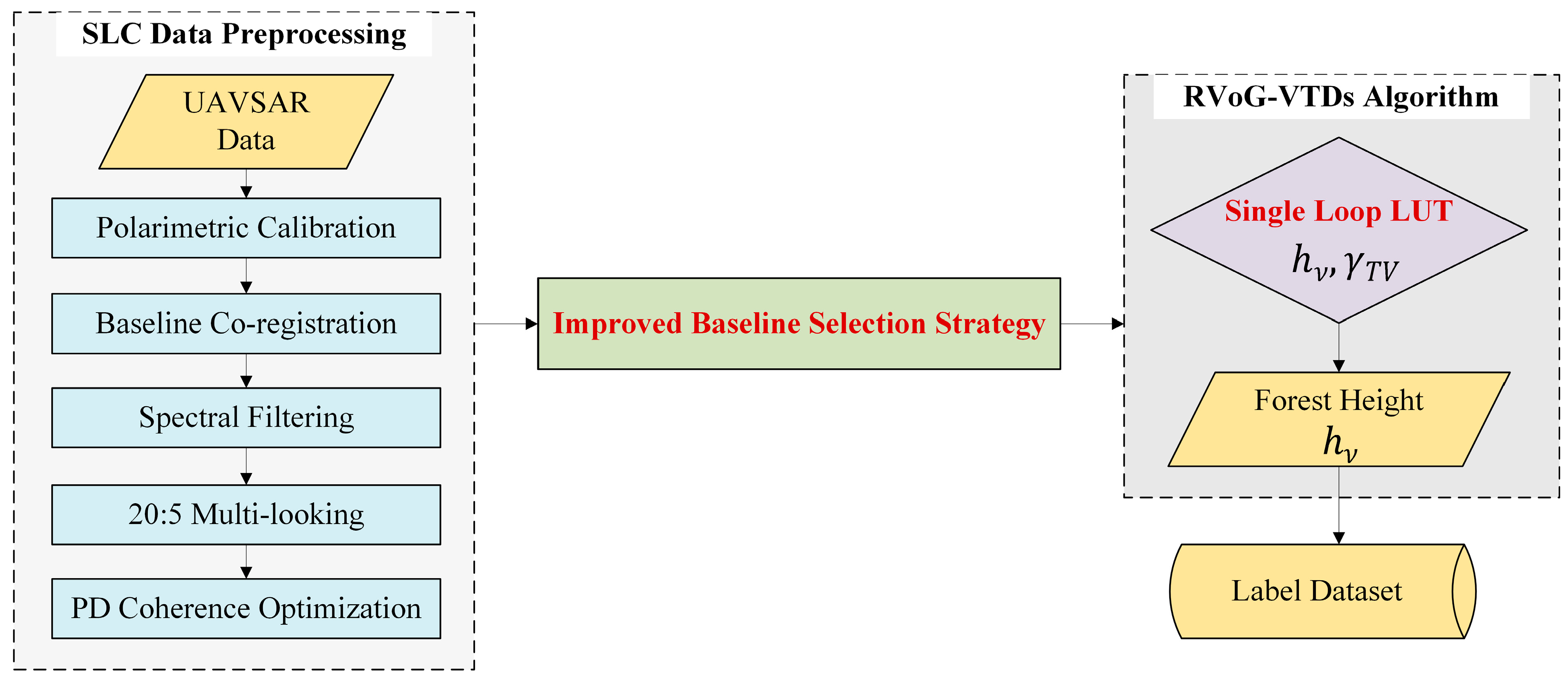
The PolInSAR data processing followed the standardized workflow recommended by the AfriSAR campaign, implemented using the open-source Python package Kapok (Version 0.2) [48,49]. The preprocessing procedures included polarimetric calibration [50], baseline co-registration [49], and spectral filtering [31,48], followed by 20:5 multilooking [49] to reduce speckle noise. Subsequently, the phase diversity (PD) optimization algorithm proposed by Tabb et al. [35] was applied to enhance coherence estimation (Table 1). The optimized coherence results were then used in conjunction with the RVoG-VTDs inversion algorithm to derive high-quality forest canopy height maps, which served as the label dataset for model training.
The LiDAR dataset consisted of synchronous LVIS RH100 products (where RH100 represents the height at which the lidar return energy reaches 100% above the ground [47]). The LVIS RH100 data from Pongara National Park were used to validate PolInSAR inversion results, while those from Akanda National Park served as ground-truth reference for testing the prediction models. To ensure the geometric consistency of validation and model training, all LiDAR datasets were reprojected to the WGS 1984 UTM Zone 32S coordinate system and resampled to a 30 m spatial resolution using the nearest-neighbor interpolation method. Subsequently, geometric co-registration was applied to align the LiDAR data spatially with the derived forest canopy height results, ensuring precise pixel-level correspondence across all datasets.

2.2.2. Multispectral and Auxiliary Data

This study integrated multi-source remote sensing datasets, projecting them to the WGS 1984 UTM Zone 32S coordinate system, resampling to a 30 m resolution, and performing pixel-level co-registration. These data captured forest growth features from multiple dimensions—spectral response, vertical structure, and topographic background (Table 2)—and were combined with PolInSAR-derived canopy height labels to train forest height prediction models.
The Landsat-8 multispectral data used in this study were obtained from the L2 products provided by the United States Geological Survey (USGS) [51]. We selected seven surface reflectance (SR) products and one land surface temperature (LST) product. Considering the impact of cloud cover during the rainy season in the study area, cloud-free images from January to June 2016 were selected. For each band, a median composite was applied to remove outliers, thereby retaining the true spectral characteristics of surface cover and maintaining spatial continuity of the data.
The spaceborne LiDAR fusion data were derived from the GEDI+Landsat global canopy height dataset released by Potapov et al. [20]. This dataset was generated by modeling GEDI L2A products containing vertical forest structural information in combination with contemporaneous Landsat-8 multispectral features, resulting in a 30 m resolution global canopy height product. In this study, the dataset was introduced as an additional structural information channel in the model input set, aiming to enhance correspondence between inputs and PolInSAR-derived labels, while also strengthening the physical interpretability of the model. Furthermore, this dataset aligns well with the multispectral data used in this study in terms of spatial and temporal scale, thereby improving data fusion performance.
The digital elevation model (DEM) data were obtained from the USGS SRTM GL1 dataset [52], which was derived from the Shuttle Radar Topography Mission (SRTM). The original spatial resolution is 30 m, and it can accurately reflect the terrain undulation characteristics of the study area.
The kNDVI was adopted as an enhanced vegetation index [53], which can better suppress soil background noise and more sensitively reflect vegetation vigor compared with the traditional NDVI. The kNDVI dataset in this study was calculated from the Landsat-8 red band and near-infrared band as follows:
N D V I = ( N I R R E D ) / ( N I R + R E D )
k N D V I = t a n h ( N D V I 2 )
where NIR refers to the near-infrared band (B5) and RED refers to the red band (B4). Finally, median compositing was applied to multi-temporal kNDVI images, and interpolation was used to fill gaps in areas with missing values, producing a complete kNDVI dataset to serve as a vegetation information channel in the model inputs.

2.3. Method

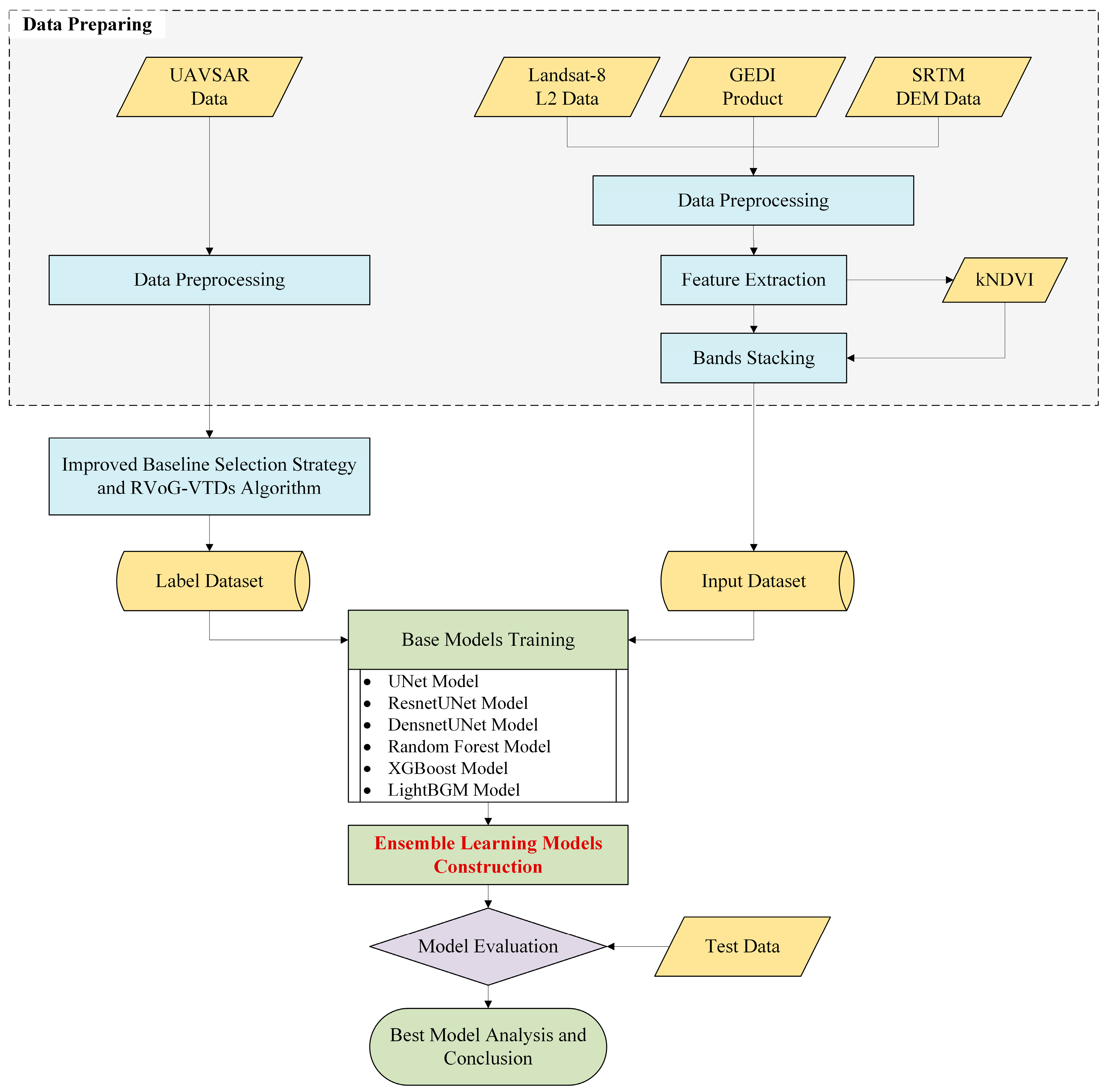
This study proposes a canopy height prediction framework based on multi-source data fusion. First, airborne PolInSAR data were processed using the RVoG-VTDs method with an improved baseline selection strategy to generate high-accuracy continuous canopy height results as the label set. These labels, together with other remote sensing feature datasets, were integrated as multi-source inputs for model training. Subsequently, an ensemble learning architecture combining machine learning and deep learning models was developed to achieve canopy height prediction and extrapolation in complex forest environments. Finally, model performance was evaluated through accuracy validation. The overall research framework is shown in Figure 2.

2.3.1. Improved Baseline Selection Strategy and RVoG-VTDs Method

The construction of the high-precision label dataset in this study primarily relied on an improved baseline selection strategy and the RVoG-VTDs forest height inversion algorithm (Figure 3).
In terms of baseline selection, Zhang et al. [45] investigated the inversion bias of multi-baseline PolInSAR across different forest height ranges and found that the applicability of various baseline selection strategies is strongly correlated with canopy height:
  • The PROD method integrates the degree of complex coherence separation and amplitude, preferentially selecting baselines with large coherence separation and high overall coherence magnitude. It performs better in low (<10 m) and tall (>30 m) forest areas, and its formulation is:
P R O D = γ h i g h γ l o w × γ h i g h + γ l o w
  • Zhang et al. [45] pointed out that in low forests (<10 m), the L-band radar signal easily penetrates the canopy and reaches the ground, leading to poor separability of the complex coherences among polarization channels and increased amplitude. The dual consideration of coherence separation and amplitude in the PROD method effectively mitigates ground scattering interference. In tall forests (>30 m), volume scattering coherence tends to saturate due to increased canopy thickness, resulting in concentrated coherence values. By emphasizing coherence amplitude stability, the PROD method reduces inversion bias caused by temporal decorrelation.
  • The ECC method (eccentricity of the coherence boundary) performs better in medium-height forests (10–30 m), where linear fitting of coherence regions is critical:
e c c = 1 ( b a ) 2
Here, a represents the major axis length of the coherence region (corresponding to coherence separation γ h i g h γ l o w ), and b is the minor axis length (the minimum boundary distance). A larger e c c indicates that the coherence region is closer to the linear assumption of the RVoG model. Zhang et al. [45] demonstrated that in medium-height forests, coherence values are more dispersed in the complex plane, and coherence amplitudes are not saturated. The linear fitting accuracy of the coherence region thus becomes crucial for inversion precision. The ECC method, which prioritizes baselines with high e c c , better characterizes the mixed scattering between the canopy and ground, achieving lower errors than the PROD method in this height range.
Based on these findings, this study proposes a PROD+ECC hybrid baseline selection strategy: applying PROD for short and tall forests to enhance accuracy, and ECC for medium-height forests to optimize linear fitting. Through regional segmentation and result mosaicking, this approach maintains the temporal decorrelation compensation advantages of RVoG-VTDs while improving adaptability across varying canopy height conditions.
For forest height inversion, the traditional RVoG model abstracts a forested area into a ground layer and a vegetation layer, assuming that ground scattering remains stable while vegetation scattering originates from randomly distributed scatterers. Their relationship is described through the overall interferometric coherence [31,32]:
γ = γ s + γ v e j φ
where γ is the overall coherence, γ s is the ground scattering coherence, γ v is the vegetation scattering coherence, and φ is the additional phase shift induced by the vegetation layer. However, this model neglects the temporal decorrelation effect in repeat-pass PolInSAR acquisitions—random motion of leaves, branches, and other scatterers during the observation interval causes coherence decay, thereby limiting inversion accuracy in complex forest environments [44].
To improve performance, Luo et al. [44] proposed the RVoG-VTDs model (Random Volume over Ground with Volumetric Temporal Decorrelation—enhanced Stochastic model). This method extends the traditional RVoG by incorporating a temporal decorrelation term ( γ T V ), which characterizes coherence decay using the probability distribution function of scatterer motion (Table 3). Its core coherence equation is expressed as follows:
γ ( ω ) = e j φ 0 γ ν γ T V + m ( ω ) 1 + m ( ω )
γ T V = e x p [ 1 2 ( 4 π λ ) 2 σ ν 2 ]
The temporal decorrelation term ( γ T V ) is the key component enabling the RVoG-VTDs model to adapt to complex forest conditions. When vegetation scatterers exhibit stronger random motion (larger σ ν ), γ T V approaches 0, resulting in more pronounced coherence decay; conversely, when motion is weaker, γ T V remains closer to 1, and coherence attenuation becomes slower [44]. Compared with the conventional RVoG model, the introduction of this parameter ensures that the retrieved canopy height labels are more robust and physically reliable across diverse forest environments.
To ensure consistency with multi-source remote sensing inputs and LiDAR data, the final continuous canopy height results were projected to the WGS 1984 UTM Zone 32S coordinate system, resampled to a 30 m spatial resolution, and geometrically co-registered with the multi-source input features. This process ensured identical spatial reference and pixel size, effectively eliminating scale discrepancies between airborne PolInSAR and satellite-based datasets, thereby providing a spatially aligned and reliable label set for subsequent model training.

2.3.2. Model Construction

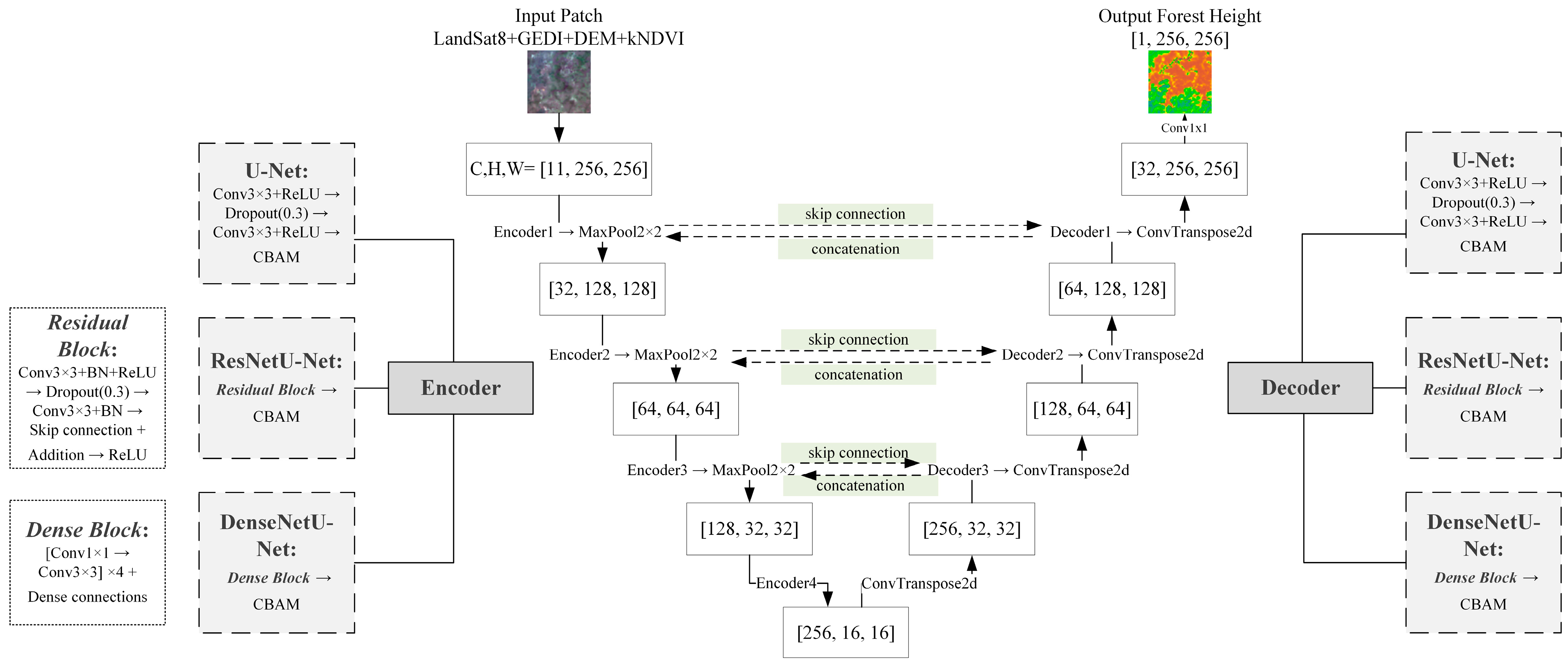
Machine learning models can automatically extract latent patterns from training data and construct predictive models with strong generalization ability, while deep learning models, with their powerful feature extraction and nonlinear fitting capacity, have shown significant advantages in remote sensing inversion tasks [54]. In this study, three representative machine learning models (RF [55], XGBoost [56], LightGBM [57]) and three deep learning models (U-Net [58], ResNetU-Net [59], DenseNetU-Net [60]) were selected as base models to construct the initial canopy height prediction framework. The machine learning models captured linear and explicit relationships among input features through ensemble tree structures, while the deep learning models (Figure 4) leveraged convolutional architectures to extract spatial nonlinear features, making the two types complementary.
For clarity and reproducibility, all key structural and training parameters of the machine learning and deep learning models used in this study are summarized in Appendix A (Table A1 and Table A2). These include the configuration of model architectures, optimization settings, loss functions, and data augmentation strategies.
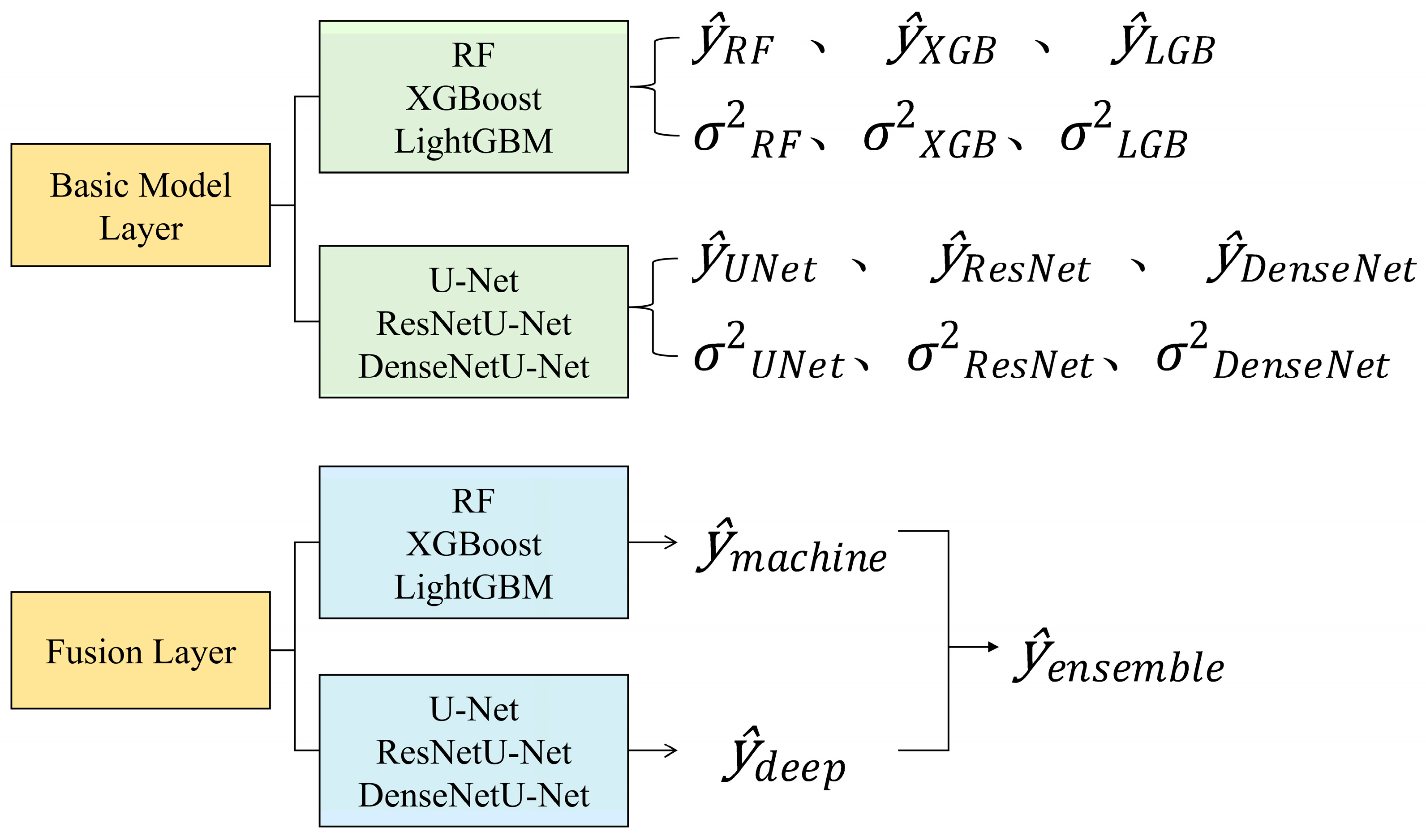
To overcome the limitations of single models in complex forest environments, we further developed a dual-layer ensemble learning framework (Figure 5). At the base-model level, the six models were trained independently and output both predictions and variance estimates. At the fusion level, a two-stage strategy was adopted: machine learning models and deep learning models were first aggregated separately using inverse-variance weighting:
ŷ m a c h i n e = m R F , X G B , L G B σ 2 m · ŷ m m R F , X G B , L G B σ 2 m
ŷ d e e p = m U N e t , R e s N e t , D e n s e N e t σ 2 m · ŷ m m U N e t , R e s N e t , D e n s e N e t σ 2 m
Finally, a dynamic weighted fusion based on prediction uncertainty was achieved by combining the two aggregated outputs with an adaptive correction factor α ( 0 , 1 ) :
ŷ e n s e m b l e = α · ŷ m a c h i n e + ( 1 α ) · ŷ d e e p
The optimization of the correction factor α was conducted using a combined strategy that minimizes the validation error while constraining local heterogeneity. The value of α is inversely correlated with the heterogeneity index H, which is computed from local variance within the sample space. Specifically, the variance of input features within each local region is first normalized to derive a heterogeneity index H [ 0 , 1 ] , where higher values indicate more complex terrain or uneven vegetation distribution, while lower values represent more homogeneous vegetation patterns. Subsequently, a grid search (step size = 0.1, range α [ 0.1 , 0.9 ] ) was performed on the validation set based on Equation (10) to identify the initial correction factor α i n i t that minimizes RMSE. Finally, a negative correlation between α i n i t and H was established to optimize α as follows:
α = α i n i t ( 1 H ) + 0.1 H
Therefore, in areas dominated by vegetation information with lower H and relatively homogeneous distribution, machine learning predictions were given higher weight ( α 1 ); whereas in complex terrains with higher H, where topographic factors dominate, deep learning predictions were prioritized ( α 0 ).
Considering the limited sample size and restricted spatial coverage, this study employed 10-Fold Cross-Validation to train and evaluate the performance of all models [61]. Specifically, the dataset was partitioned into ten independent subsets based on spatial correlation, ensuring that the training and validation sets were spatially non-overlapping, thereby effectively avoiding overfitting and information leakage. The mean performance across the ten folds was used as the evaluation and optimization metric on the validation sets. After training, the average of the fold-specific weights for each model was adopted as the final prediction result.

2.3.3. Accuracy Validation

This study adopted the coefficient of determination (R2), root mean square error (RMSE), and mean absolute error (MAE) as evaluation metrics to assess accuracy. The inversion accuracy of PolInSAR was compared with LVIS RH100, and further cross-regional independent testing was conducted in Akanda National Park to validate the predictive performance of both base models and the ensemble model. The formulas are as follows:
B I A S = 1 N i = 1 N ( E i M i )
R M S E = 1 N i = 1 N ( E i M i ) 2
R 2 = 1 i = 1 N ( E i M i ) 2 i = 1 N ( E i M ¯ ) 2
where N is the total number of samples, i denotes a single observation, M and E represent the measured and estimated values, respectively, and M ¯ is the mean of the measured values.

3. Results

3.1. Analysis and Comparison of Label Set Inversion Results

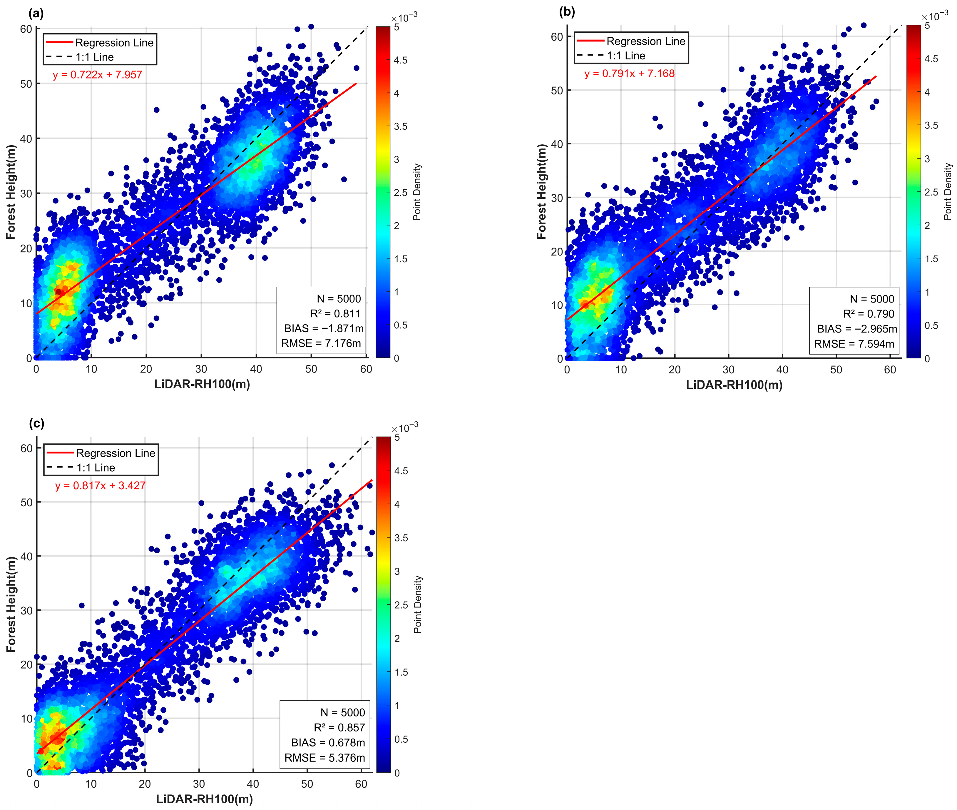
This study employed the RVoG-VTDs method, with an improved baseline selection strategy and subsequent result mosaicking, to perform forest height inversion on the PolInSAR dataset from Pongara National Park. The LVIS RH100 data, after co-registration, were used as reference measurements for accuracy assessment. A total of 5000 sample points were collected, yielding the results presented in Table 4 and Figure 6 and Figure 7.
Comparison of the three baseline selection methods combined with RVoG-VTDs shows that the PROD-only method achieved an R2 of 0.811, a BIAS of −1.871 m, and an RMSE of 7.176 m. The ECC-only method yielded an R2 of 0.790, a BIAS of −2.965 m, and an RMSE of 7.594 m. These results indicate that in this study area, where low and tall forest stands dominate, the PROD method performed relatively better, indirectly confirming the structural complexity of the forest scene.
In contrast, the proposed hybrid baseline method achieved an R2 of 0.857, a BIAS of 0.678 m, and reduced the RMSE to 5.376 m. Our strategy reduced RMSE by 25%, and this demonstrates a significant improvement in accuracy compared with the single-method approaches. Moreover, Figure 6 shows that the residual distribution under the adaptive method was more uniform, with the fitted regression line closer to the 1:1 line, indicating enhanced stability. Figure 7 further illustrates that the mean and standard deviation of errors were smaller, and the probability of low-error samples was higher.
Overall, these findings confirm that the adaptive baseline method proposed in this study produced more accurate and stable inversion results compared with single baseline selection strategies. Therefore, it is more suitable to serve as the label dataset for subsequent model training.

3.2. Analysis and Comparison of Model Prediction Results

To validate the feasibility of using PolInSAR-derived forest canopy height results as label sets for training and constructing large-scale forest height prediction models, this study employed six base models and one ensemble model. Model training and tuning were conducted in the training area (Pongara National Park), while predictions and accuracy assessments were performed in the testing area (Akanda National Park).

3.2.1. Visualization of Model Prediction Results

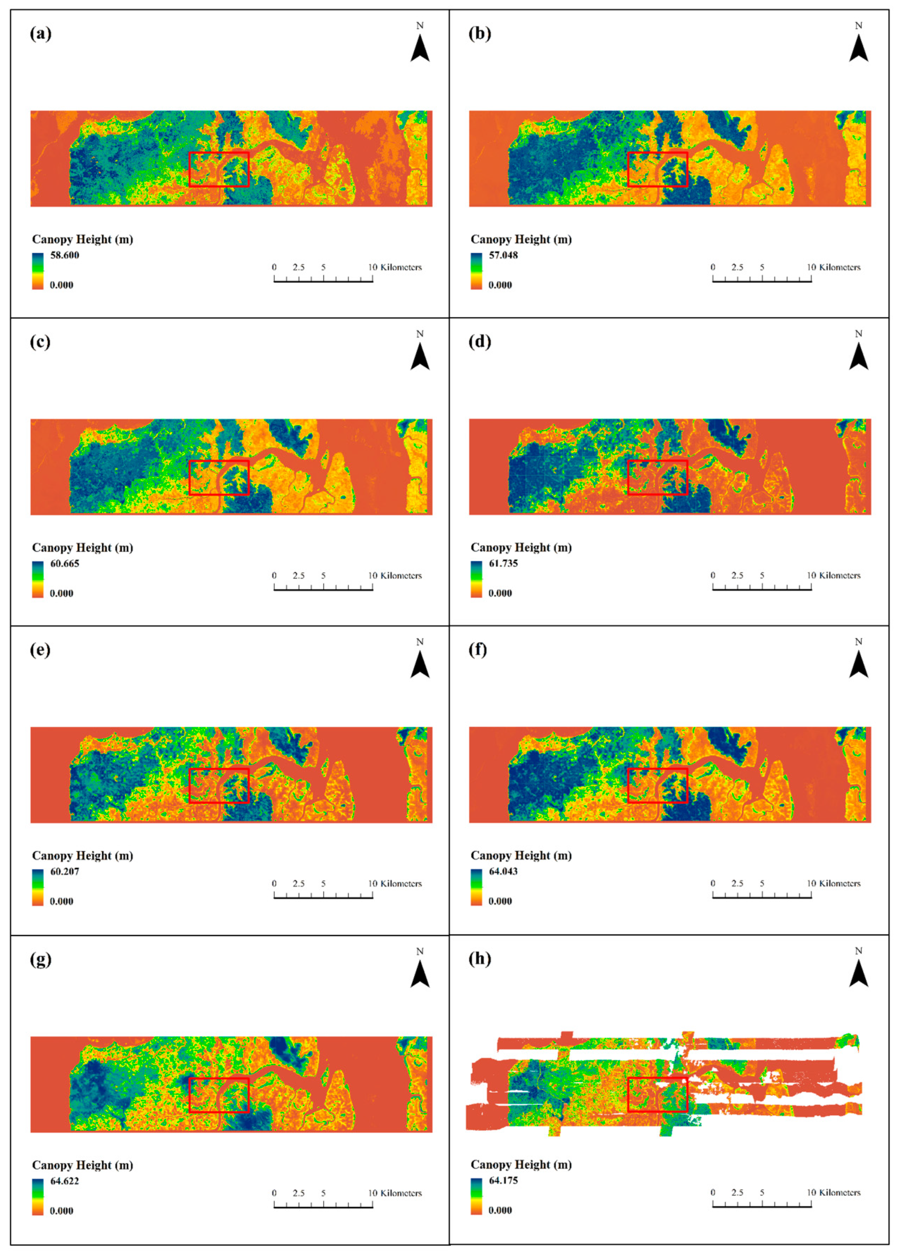
Figure 8 shows the overall prediction results of the six base models and the ensemble learning model in the testing area. Compared with the LVIS RH100 LiDAR data, the RF and XGBoost models significantly underestimated extremely high values, while the DenseNetU-Net model’s predictions for extreme values were closer to the observed data. In addition, machine learning models tended to produce prediction noise in large non-forest areas, with noise severity decreasing from RF to XGBoost to LightGBM. In contrast, among the deep learning models, only DenseNetU-Net exhibited a certain degree of noise in similar areas. However, because the deep learning models were trained on small patch samples rather than single-pixel feature vectors, they showed varying degrees of detail loss and slight stitching artifacts. The U-Net model was most affected, with substantial detail loss, whereas ResNetU-Net and DenseNetU-Net were less impacted. Meanwhile, the ensemble learning model, by integrating all base models, not only achieved predictions of extreme values closer to the observations but also largely eliminated noise interference and detail loss.
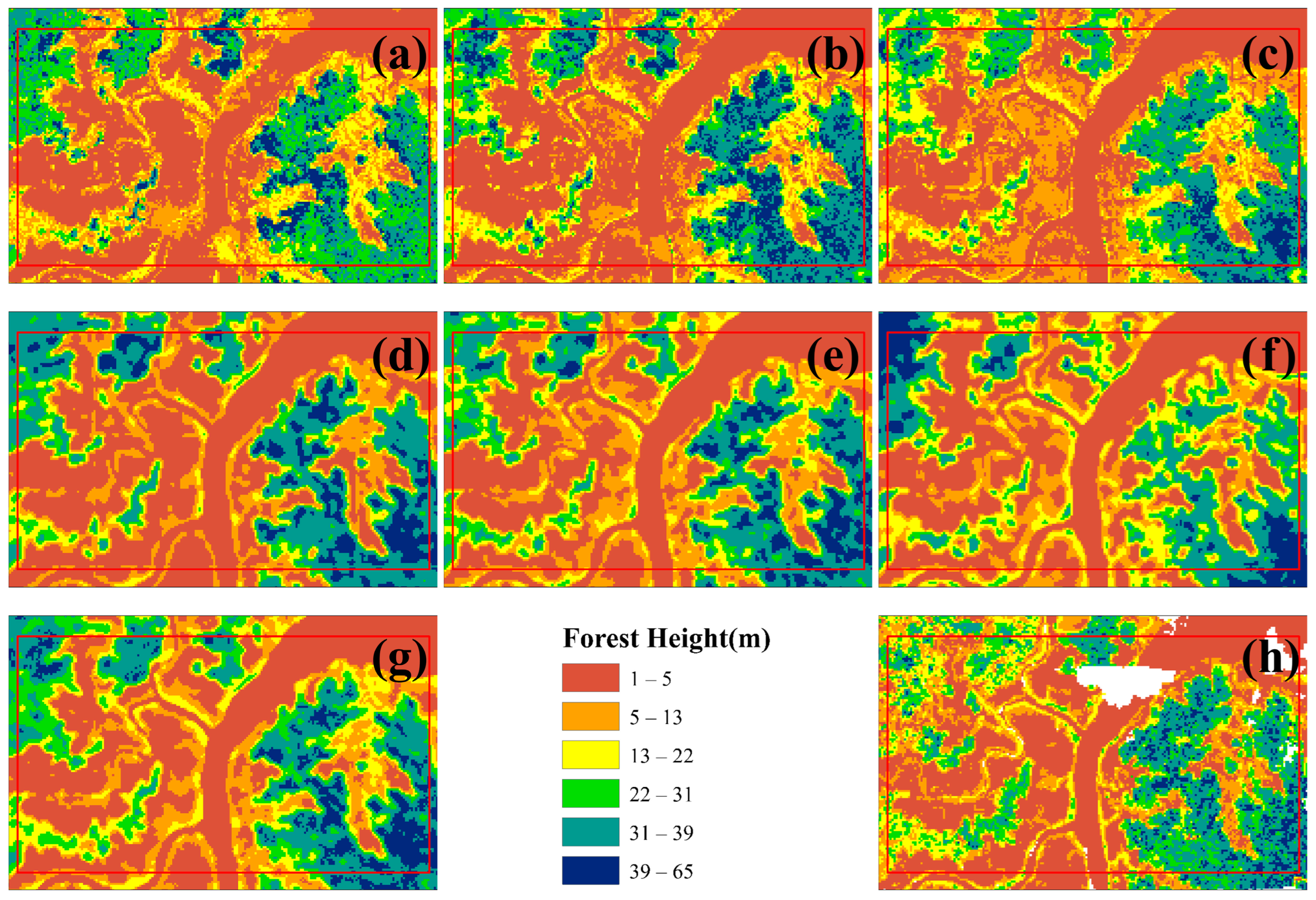
Figure 8 and Figure 9 further illustrates local details after unifying the color scale. Compared with observed data, the machine learning models, which relied on single-pixel feature vectors for training and prediction, were more prone to noise in local predictions, with RF showing the most significant noise. By contrast, deep learning models produced smoother predictions with fewer details lost. Notably, ResNetU-Net, which captured details through residual connections, and DenseNetU-Net, which captured deeper terrain information through dense connections, showed prediction shapes and average distributions closer to the observed data. A comparative analysis revealed that machine learning models aligned better with observations in the mid-height range (13–31 m, corresponding to yellow and green in the legend), whereas deep learning models were more accurate in low and tall canopy regions. Finally, the ensemble learning model preserved local details, avoided noise, and achieved the closest prediction to the observed forest canopy height distribution, effectively combining the strengths of both machine learning and deep learning models.

3.2.2. Comparison and Analysis of Prediction Accuracy

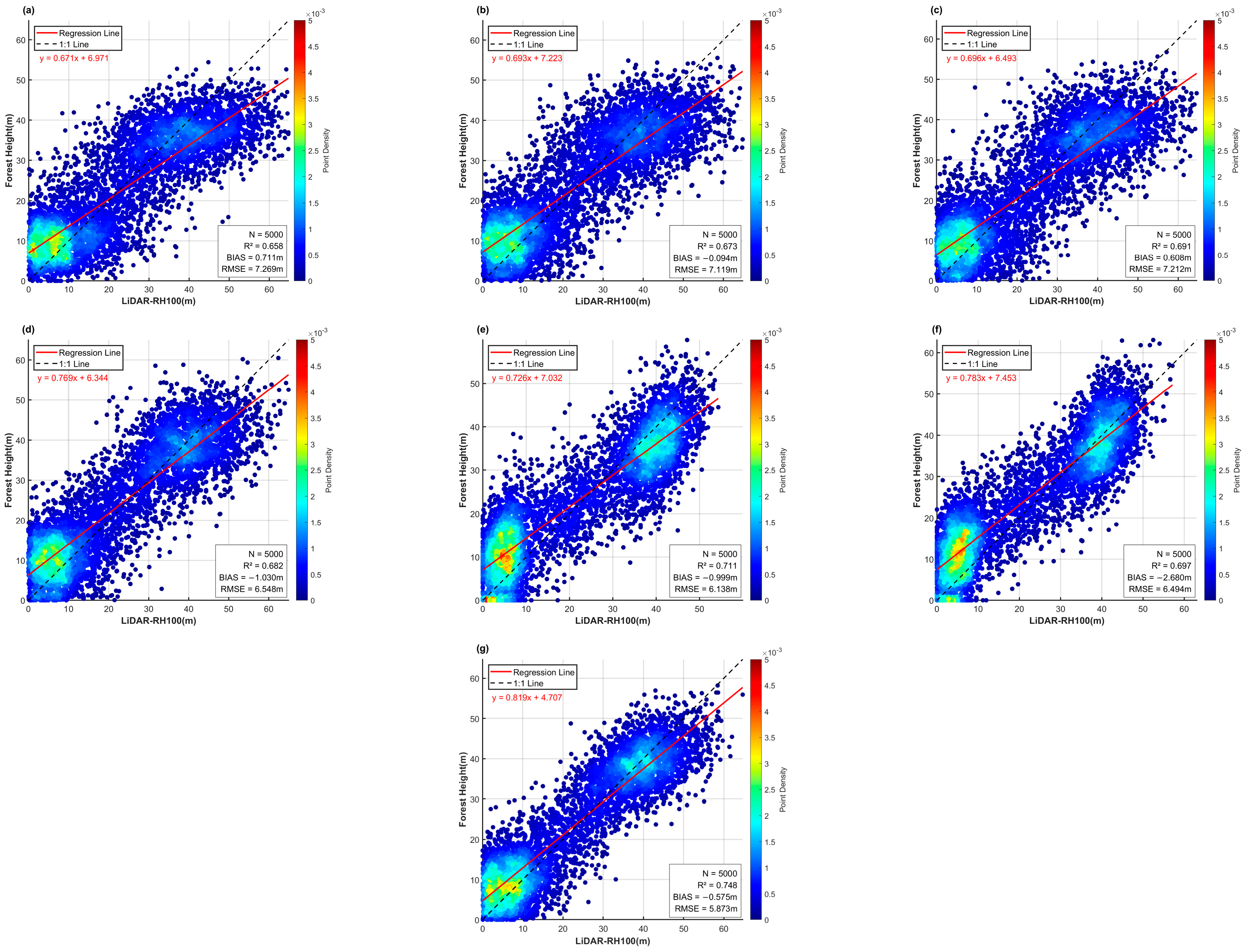
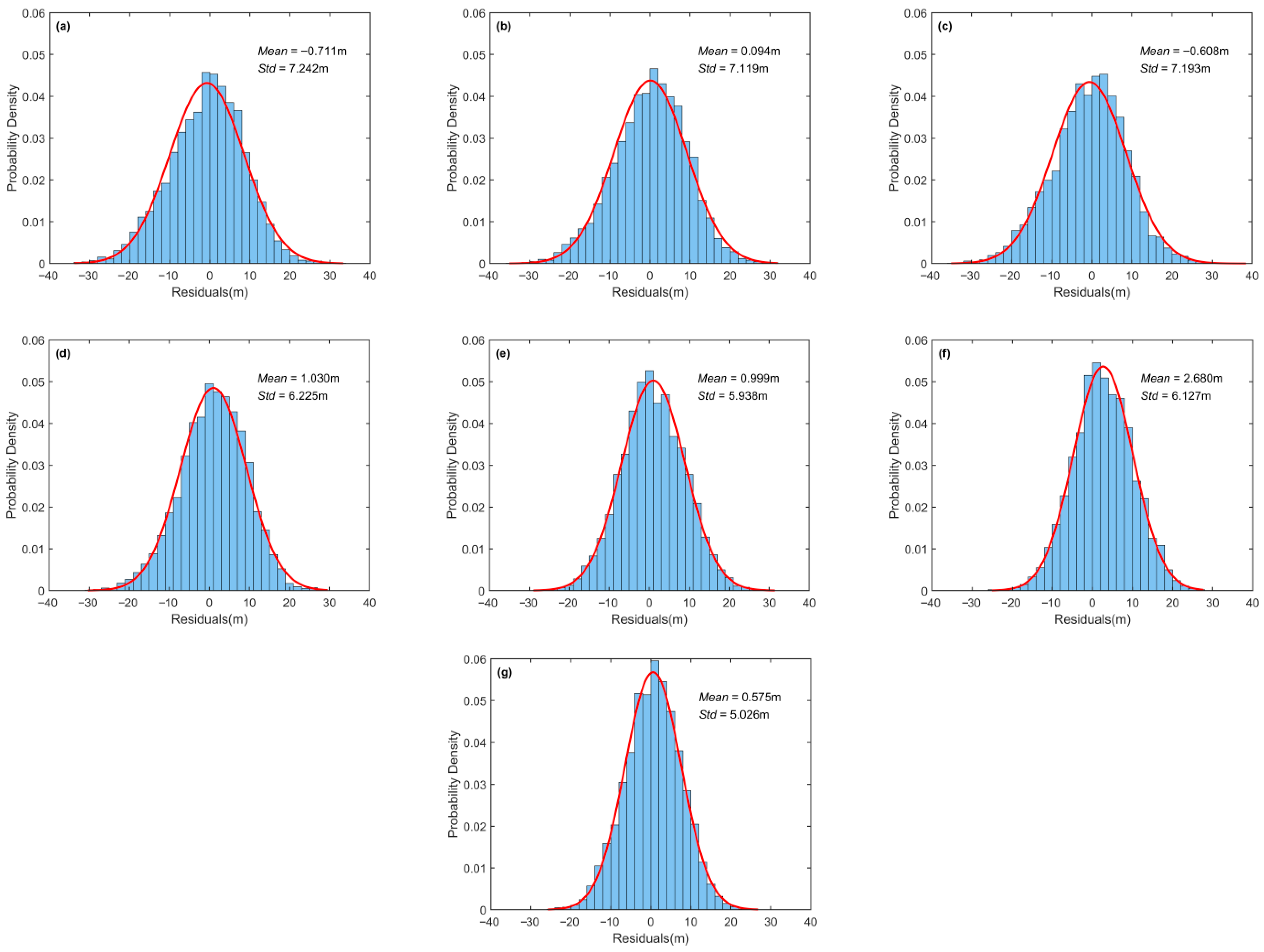
Figure 10 and Figure 11 present the accuracy evaluation of the six base models and the ensemble learning model in the testing area. The results show that deep learning models generally had smaller prediction errors and better stability than machine learning models, consistent with the conclusions from Section 3.2.1. Among the base models, ResNetU-Net performed best, reducing RMSE to 6.138 m, lowering the error standard deviation to 5.938 m, and achieving an R2 of 0.711. These findings also aligned with its superior visualization performance in Section 3.2.1. Moreover, the ensemble model consistently reduced errors and improved stability compared with each base model. Specifically, it achieved an RMSE of 5.873 m and an R2 of 0.748, both superior to all base models. The error standard deviation of the ensemble model was as low as 5.026 m, and its residual histogram indicated a higher probability of small-error samples. These results confirm that the proposed ensemble model achieved the best overall performance.

3.2.3. Comparison with Existing Global Models

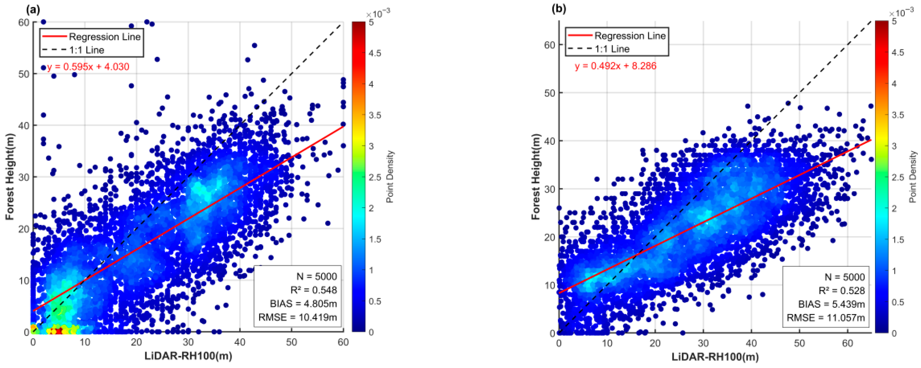
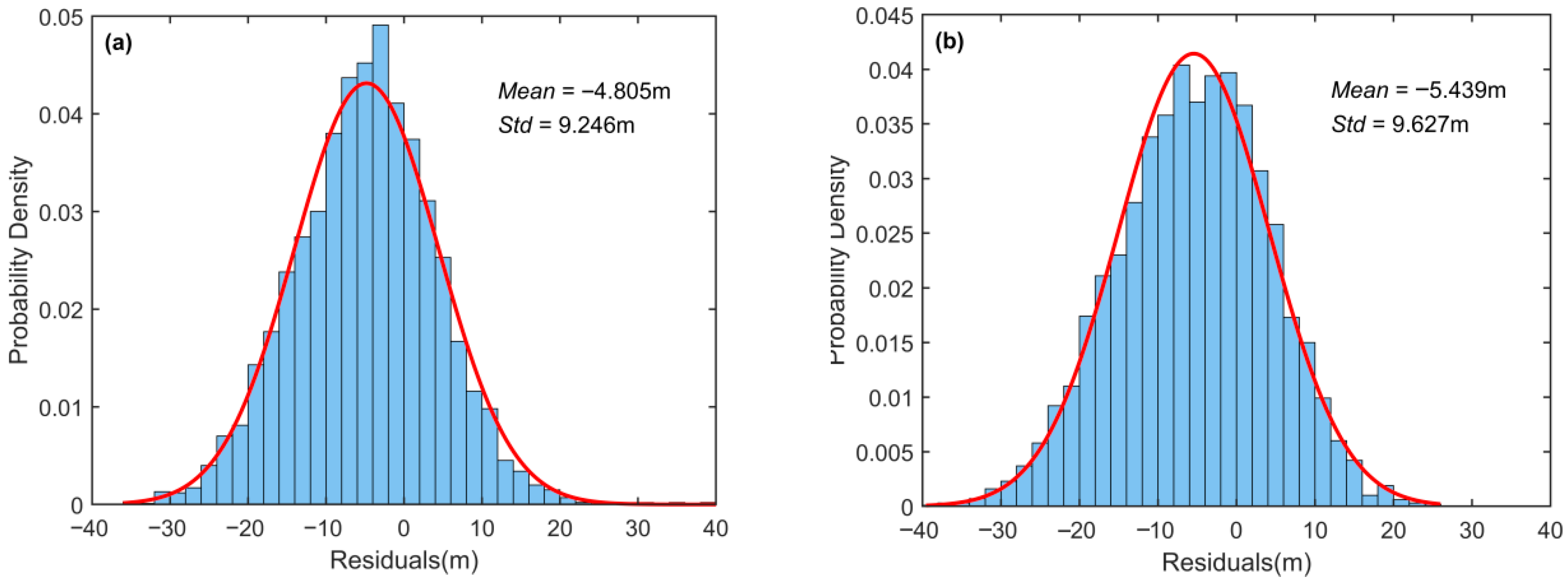
Due to the limited availability of GEDI LiDAR footprint samples in the study area, training the proposed model using GEDI data alone as the label set failed to achieve convergence. This indirectly demonstrates the unique advantage of the label set employed in this study for small-scale forest canopy height estimation. Therefore, in Table 5, Figure 12 and Figure 13, we directly compared the prediction accuracy of two publicly available global canopy height datasets, both of which used GEDI LiDAR data as labels with large sample sizes. Potapov et al. [20] employed Landsat-8, NDVI, and DEM as inputs to train machine learning models, while Lang et al. [21] used Sentinel-2 data as inputs for deep learning models. Although both models achieved good accuracy at the global scale (Table 6)—Potapov et al. [20] reported RMSE = 9.07 m, MAE = 6.36 m, R2 = 0.61, and Lang et al. [21] reported RMSE = 6.0 m, MAE = 4.0 m—their performance weakened in local areas such as our study site. Both models exhibited significant underestimation in our testing region. This indicates that when the research objective is to obtain more accurate canopy height mapping and prediction at local scales, the ensemble learning approach proposed in this study is more suitable.

3.3. Analysis of Model Channel Sensitivity Results

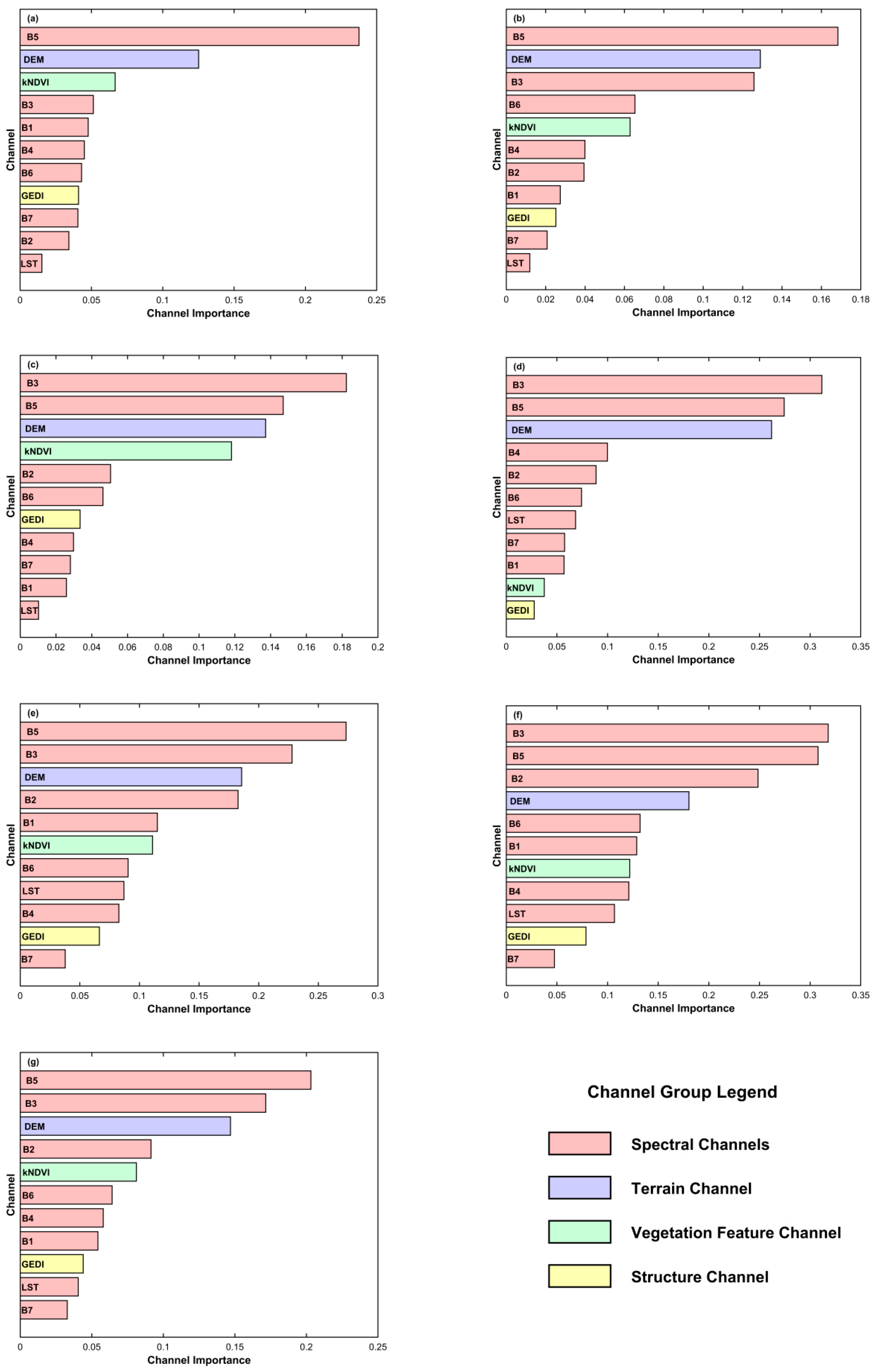
Figure 14 presents the contributions of different channels to the importance ranking during training for the six base models and the ensemble learning model in this study. For Landsat 8 data, bands B1 to B7 correspond to Coastal aerosol, Blue, Green, Red, NIR, SWIR 1, and SWIR 2 channels, respectively (Table 2).
Specifically, for machine learning models, the common key channels are vegetation related spectral bands (Green, NIR), the vegetation feature channel (kNDVI), and the topographic feature channel (DEM). In contrast, for deep learning models, the most important channels are primarily Green, NIR, and DEM, while the relative importance of the vegetation feature channel (kNDVI) decreases. Notably, for both categories of base models, the GEDI channel containing canopy height information ranks lower in importance; however, in machine learning models, GEDI ranks slightly higher than in deep learning models.
The reason for the relatively lower importance of kNDVI and GEDI in deep learning models may lie in their different mechanisms of feature extraction. Machine learning models analyze the numerical correlation between pixel feature vectors and target values, with more complex models better able to capture mathematical relationships. By contrast, deep learning models rely on a dual loss function combining numerical error (MSE) and structural similarity error (SSIM) to capture spatial similarity across patches. Combined with the visualization results in Section 3.2.1, it is evident that deep learning models tend to capture structural and mean-value trends, which likely contributes to the reduced importance of kNDVI and GEDI channels. Meanwhile, since the GEDI channel in this study is derived from the global GEDI dataset released by Potapov et al. [22], together with the accuracy validation results for this dataset in our study area (Section 3.2.2), it is reasonable to infer that the lower contribution of GEDI channels across models may be partly due to the inherent accuracy limitations of the dataset itself.
Overall, in the ensemble learning model that integrates all base models, the pattern of channel importance remains consistent with that of the individual models. The commonly shared key channels include vegetation-related spectral bands (Green and NIR), the topographic channel (DEM), and the vegetation feature channel (kNDVI), while the least contributing channels are the land surface temperature (LST) and the longer-wavelength shortwave infrared bands.

4. Discussion

This study proposed an ensemble learning framework that integrates airborne PolInSAR-derived canopy height labels with multi-source remote sensing data to address the uncertainty of sparse LiDAR-based models in heterogeneous tropical forests. Compared with conventional interpolation-dependent methods, this framework generates continuous high-quality labels and adaptively fuses complementary features across spectral, structural, and topographic dimensions.
The key advantage of PolInSAR over traditional remote sensing techniques lies in its ability to accurately characterize vertical canopy structure. By jointly exploiting polarization and interferometric information, PolInSAR can effectively separate surface and vegetation scattering components and capture vertical height differences through interferometric phase analysis, providing unique advantages in structurally complex tropical mangrove environments such as those in Gabon. The airborne L-band radar used in this study provides strong canopy penetration capability, forming a continuous scattering profile from the canopy top to the ground. While the RVoG-VTDs model introduces a temporal decorrelation term ( γ T V ) to quantify coherence loss caused by random leaf and branch motion, and this enables more accurate separation of canopy and ground phases, reducing the bias of conventional RVoG models that often misinterpret temporal decorrelation as canopy thickness [44].
Furthermore, the proposed hybrid baseline strategy (PROD+ECC) optimizes baseline selection across different canopy height ranges. The PROD method enhances inversion stability in tall forests (>30 m) with large coherence separation between canopy- and ground-dominated components ( γ h i g h , γ l o w ) and in short forests (<10 m) with low separation, while the ECC method improves performance in mid-height forests (10–30 m) by selecting baselines with higher linearity [45]. Experiments demonstrated that this strategy increased inversion accuracy by about 25%, confirming that a multi-baseline approach based on canopy height stratification can effectively mitigate errors caused by signal saturation or coherence ambiguity.
This study also integrates optical, LiDAR, topographic, and vegetation index features (Table 2) to jointly capture canopy height variation from spectral, structural, and terrain perspectives. Channel importance analysis showed that vegetation-related spectral bands (Green, NIR), terrain elevation (DEM), and the enhanced vegetation index (kNDVI) contributed most across models. Physically, the Green band (B3) relates to chlorophyll content and canopy vigor, aiding the distinction between young and mature stands [8]; the NIR band (B5), controlled by leaf cellular structure, correlates with leaf area index and indirectly indicates canopy thickness [8]; DEM represents terrain variation, correcting reflectance distortions and reflecting growth constraints such as reduced canopy height on steep slopes [52]; and kNDVI, less affected by soil background and saturation at high biomass, effectively differentiates canopy developmental stages [53].
Notably, the GEDI-derived vertical structure data contributed less to local model performance, likely due to systematic biases of global products at finer spatial scales (RMSE > 10 m). Deep learning models showed lower dependence on GEDI and kNDVI than machine learning models, probably because they autonomously extract spatial and contextual structure from raw spectral and terrain inputs rather than relying on predefined indices or secondary products.
Compared with the global canopy height products by Potapov et al. [20] and Lang et al. [21], the proposed method achieved lower RMSE (5.87 m) and higher R2 (0.748) in the local test region. This improvement arises from three key factors: (1) Label enhancement—PolInSAR-derived continuous labels reached RMSE = 5.38 m and R2 = 0.857 in the Pongara area, reducing error propagation from heterogeneous and interpolated GEDI/ICESat-2 footprints; (2) Model architecture optimization—the dual-layer ensemble dynamically balances the spectral sensitivity of machine learning and the structural perception of deep learning, achieving bias < 1 m compared with >4 m in Potapov et al. [20] and Lang et al. [21]; and (3) Feature refinement—in contrast to Potapov et al. [20] and Lang et al. [21], this study incorporated more physically grounded inputs such as DEM, GEDI, and kNDVI, which jointly enhanced model accuracy.
Nevertheless, our study has certain limitations. First, the experimental area was restricted to the PolInSAR coverage in Gabon; broader validation is needed to test generalizability across other forest types. Second, the diversity of multisource inputs was limited; incorporating additional features such as climate variables and SAR polarimetric indices may further enhance interpretability and robustness. Third, while PolInSAR inversion labels avoid the drawbacks of interpolation and sparse supervision, error propagation remains an issue; thus, exploring alternative or improved label sources is essential. Notably, the recent launch of ESA’s BIOMASS P-band SAR satellite offers new opportunities [62], as it will provide more penetrating and accurate forest parameters, including canopy height and biomass. Such datasets are expected to help overcome current limitations in data coverage, type, and accuracy, enabling more robust forest monitoring.
In conclusion, our study represents an attempt to construct novel labels based on airborne PolInSAR canopy height inversion, combined with multi-source remote sensing data to build and integrate multiple training models. The objective is to develop a canopy height prediction framework that does not rely on discontinuous LiDAR labels, thereby enabling applications in locally complex forest environments. The proposed ensemble learning model demonstrates optimal performance under the current study area and data availability. With the continuous accumulation of PolInSAR data and the incorporation of emerging satellite observations in the future, the model will be further refined and updated. We will continue to optimize the framework to achieve higher stability, improved accuracy, and stronger generalization capability in forest canopy height prediction.
5. Conclusions

This study developed a canopy height prediction framework that integrates airborne PolInSAR-derived continuous labels with multi-source remote sensing features through a dual-layer ensemble learning model. The hybrid PROD+ECC baseline strategy significantly improved inversion accuracy, enabling PolInSAR labels to serve as a reliable alternative to sparse LiDAR samples. By combining spectral, structural, and topographic information, the ensemble model achieved superior performance in complex tropical forests and outperformed existing global canopy height products in independent validation. Although the method is currently constrained by the spatial coverage of available PolInSAR data, the rapid expansion of PolInSAR observations and future missions such as ESA’s BIOMASS satellite will further enhance its applicability. Overall, this study provides an effective and scalable pathway for improving canopy height estimation and contributes to advancing forest carbon stock assessment and ecological monitoring.

Author Contributions

Conceptualization, Y.L. and X.Z.; methodology, Y.L.; software, Y.L. and W.C.; validation, Y.L.; formal analysis, Y.L. and T.L.; investigation, Y.L. and H.Z.; data curation, Y.L., Z.T. and W.C.; writing—original draft preparation, Y.L.; writing—review and editing, Y.L., X.Z. and T.L.; visualization, Y.L.; supervision, X.Z., T.L. and Z.T.; project administration, X.Z.; funding acquisition, X.Z. All authors have read and agreed to the published version of the manuscript.

Funding

This research was supported by the National Key Research and Development Program of China (Grant No. 2023YFB3907705).

Data Availability Statement

The data can be sourced from the following providers: The Landsat-8 Surface Reflectance data, and the SRTM-DEM product are available through Google Earth Engine (https://developers.google.com/earth-engine/datasets/, accessed on 16 June 2025). The UAVSAR data can be downloaded from NASA Jet Propulsion Laboratory (https://uavsar.jpl.nasa.gov/). The LVIS RH100 LiDAR data can be downloaded from NASA Earth Science Data (https://www.earthdata.nasa.gov/data/catalog/ornl-cloud-afrisar-lvis-biomass-vprofiles-1775-1, accessed on 21 May 2025). The GEDI and Landsat fusion product can be downloaded from Global Land Analysis & Discovery (https://glad.umd.edu/dataset/gedi/ or https://aws.amazon.com/marketplace/pp/prodview-elqs43227adgw?sr=0-1&ref_=beagle&applicationId=AWSMPContessa#resources, accessed on 19 November 2025).

Acknowledgments

We would like to express our gratitude to the teams behind the Google Earth Engine platform for providing access to essential remote sensing datasets. We also extend our appreciation to the NASA AfriSAR team for providing the open access to UAVSAR data and airborne LiDAR data. Special gratitude to the GEDI and GLAD teams for making their spaceborne lidar products accessible.

Conflicts of Interest

The authors declare no conflicts of interest.

Abbreviations

The following abbreviations are used in this manuscript:
PolInSARPolarimetric SAR Interferometry
LiDARLight Detection and Ranging
GEDIGlobal Ecosystem Dynamics Investigation
RFRandom Forest
XGBoostExtreme Gradient Boosting
LightGBMLight Gradient Boosting Machine
RVoGRandom Volume over Ground

Appendix A. Model Parameter Configurations

The following tables summarize the detailed configurations of the machine learning and deep learning models used in this study.
Table A1. Parameter Configuration of Machine Learning Models.
ModelParameter CategorySpecific Parameters and Values
Random Forest (RF)Structural ParametersNumber of decision trees = 200; Maximum tree depth = 25; Minimum samples per leaf node = 5
Training ParametersParallel computing: Random seed fixed (seed = 42)
XGBoostStructural ParametersNumber of decision trees = 200; Maximum tree depth = 8; Regularization parameters (reg_lambda = 0.5, reg_alpha = 0.1)
Training ParametersLearning rate = 0.05; Tree construction method = “hist”; GPU acceleration; Early stopping (patience = 20)
LightGBMStructural ParametersNumber of decision trees = 300; Maximum tree depth = 6; Regularization parameters (reg_lambda = 2.0, reg_alpha = 0.1)
Training ParametersLearning rate = 0.1; Feature sampling; Early stopping (patience = 20)
Table A2. Parameter Configuration of Deep Learning Models.
ModelParameter CategorySpecific Parameters and Values
U-NetStructural ParametersKernel size = 3 × 3; Encoder/decoder layers = 4 each; With CBAM attention module
Training ParametersLearning rate = 3 × 10⁻⁴; Weight decay = 1 × 10⁻⁵; Learning rate scheduler = ReduceLROnPlateau; Epochs = 100; Loss function = 0.8 × MSE + 0.2 × SSIM
ResNetU-NetStructural ParametersEncoder/decoder module = Residual block (2 layers of 3 × 3 convolution + BN + ReLU + skip connection); With CBAM attention module
Training ParametersLearning rate scheduler = OneCycleLR; Learning rate = 2 × 10⁻⁴; Epochs = 200; Loss function = 0.6 × MSE + 0.4 × SSIM
DenseNetU-NetStructural ParametersEncoder/decoder module = Dense block (4 layers of 1 × 1 + 3 × 3 convolution + feature concatenation); Growth rate = 16; With CBAM attention module
Training ParametersLearning rate = 5 × 10⁻⁴; Learning rate scheduler = ReduceLROnPlateau; Epochs = 150; Loss function = 0.8 × MSE + 0.2 × SSIM
All Deep Learning ModelsCommon ParametersOptimizer = Adam; Encoder channels = 11 → 32 → 64 → 128; Output channels = 1; Patch size = 32 × 32; Batch size = 32
Data AugmentationRandom brightness/contrast adjustment (probability = 0.5); Gaussian noise addition (standard deviation = 0.001–0.01, probability = 0.5)

References

  1. Beer, C.; Reichstein, M.; Tomelleri, E.; Ciais, P.; Jung, M.; Carvalhais, N.; Rödenbeck, C.; Arain, M.A.; Baldocchi, D.; Bonan, G.B.; et al. Terrestrial Gross Carbon Dioxide Uptake: Global Distribution and Covariation with Climate. Science 2010, 329, 834–838. [Google Scholar] [CrossRef]
  2. Pan, Y.; Birdsey, R.A.; Fang, J.; Houghton, R.; Kauppi, P.E.; Kurz, W.A.; Phillips, O.L.; Shvidenko, A.; Lewis, S.L.; Canadell, J.G.; et al. A Large and Persistent Carbon Sink in the World’s Forests. Science 2011, 333, 988–993. [Google Scholar] [CrossRef]
  3. Skidmore, A.K.; Coops, N.C.; Neinavaz, E.; Ali, A.; Schaepman, M.E.; Paganini, M.; Kissling, W.D.; Vihervaara, P.; Darvishzadeh, R.; Feilhauer, H. Priority List of Biodiversity Metrics to Observe from Space. Nat. Ecol. Evol. 2021, 5, 896–906. [Google Scholar] [CrossRef] [PubMed]
  4. Tuanmu, M.-N.; Jetz, W. A Global, Remote Sensing-Based Characterization of Terrestrial Habitat Heterogeneity for Biodiversity and Ecosystem Modelling. Glob. Ecol. Biogeogr. 2015, 24, 1329–1339. [Google Scholar] [CrossRef]
  5. Zhou, X.; Pan, J.; Wu, Y. Transparent Earth-Observing: Exploring the New Generation of Earth Observation Technology. Natl. Remote Sens. Bull. 2024, 28, 529–540. [Google Scholar] [CrossRef]
  6. Chirici, G.; Chiesi, M.; Corona, P.; Salvati, R.; Papale, D.; Fibbi, L.; Sirca, C.; Spano, D.; Duce, P.; Marras, S.; et al. Estimating Daily Forest Carbon Fluxes Using a Combination of Ground and Remotely Sensed Data. J. Geophys. Res. Biogeosci. 2016, 121, 266–279. [Google Scholar] [CrossRef]
  7. Chen, W.; Zheng, Q.; Xiang, H.; Chen, X.; Sakai, T. Forest Canopy Height Estimation Using Polarimetric Interferometric Synthetic Aperture Radar (PolInSAR) Technology Based on Full-Polarized ALOS/PALSAR Data. Remote Sens. 2021, 13, 174. [Google Scholar] [CrossRef]
  8. Rodríguez-Veiga, P.; Wheeler, J.; Louis, V.; Tansey, K.; Balzter, H. Quantifying Forest Biomass Carbon Stocks from Space. Curr. For. Rep. 2017, 3, 1–18. [Google Scholar] [CrossRef]
  9. Huete, A.; Didan, K.; Miura, T.; Rodriguez, E.P.; Gao, X.; Ferreira, L.G. Overview of the Radiometric and Biophysical Performance of the MODIS Vegetation Indices. Remote Sens. Environ. 2002, 83, 195–213. [Google Scholar] [CrossRef]
  10. Asner, G.P.; Keller, M.; Silva, J.N.M. Spatial and Temporal Dynamics of Forest Canopy Gaps Following Selective Logging in the Eastern Amazon. Glob. Change Biol. 2004, 10, 765–783. [Google Scholar] [CrossRef]
  11. Dubayah, R.; Blair, J.B.; Goetz, S.; Fatoyinbo, L.; Hansen, M.; Healey, S.; Hofton, M.; Hurtt, G.; Kellner, J.; Luthcke, S.; et al. The Global Ecosystem Dynamics Investigation: High-Resolution Laser Ranging of the Earth’s Forests and Topography. Sci. Remote Sens. 2020, 1, 100002. [Google Scholar] [CrossRef]
  12. Magruder, L.A.; Brunt, K.M.; Alonzo, M. Early ICESat-2 on-Orbit Geolocation Validation Using Ground-Based Corner Cube Retro-Reflectors. Remote Sens. 2020, 12, 3653. [Google Scholar] [CrossRef]
  13. Neuenschwander, A.; Pitts, K. The ATL08 Land and Vegetation Product for the ICESat-2 Mission. Remote Sens. Environ. 2019, 221, 247–259. [Google Scholar] [CrossRef]
  14. Magruder, L.A.; Brunt, K.M. Performance Analysis of Airborne Photon- Counting Lidar Data in Preparation for the ICESat-2 Mission. IEEE Trans. Geosci. Remote Sens. 2018, 56, 2911–2918. [Google Scholar] [CrossRef]
  15. Markus, T.; Neumann, T.; Martino, A.; Abdalati, W.; Brunt, K.; Csatho, B.; Farrell, S.; Fricker, H.; Gardner, A.; Harding, D.; et al. The Ice, Cloud, and Land Elevation Satellite-2 (ICESat-2): Science Requirements, Concept, and Implementation. Remote Sens. Environ. 2017, 190, 260–273. [Google Scholar] [CrossRef]
  16. Sothe, C.; Gonsamo, A.; Lourenço, R.B.; Kurz, W.A.; Snider, J. Spatially Continuous Mapping of Forest Canopy Height in Canada by Combining GEDI and ICESat-2 with PALSAR and Sentinel. Remote Sens. 2022, 14, 5158. [Google Scholar] [CrossRef]
  17. Hansen, M.C.; Potapov, P.V.; Goetz, S.J.; Turubanova, S.; Tyukavina, A.; Krylov, A.; Kommareddy, A.; Egorov, A. Mapping Tree Height Distributions in Sub-Saharan Africa Using Landsat 7 and 8 Data. Remote Sens. Environ. 2016, 185, 221–232. [Google Scholar] [CrossRef]
  18. Matasci, G.; Hermosilla, T.; Wulder, M.A.; White, J.C.; Coops, N.C.; Hobart, G.W.; Zald, H.S.J. Large-Area Mapping of Canadian Boreal Forest Cover, Height, Biomass and Other Structural Attributes Using Landsat Composites and Lidar Plots. Remote Sens. Environ. 2018, 209, 90–106. [Google Scholar] [CrossRef]
  19. Silva, C.A.; Duncanson, L.; Hancock, S.; Neuenschwander, A.; Thomas, N.; Hofton, M.; Fatoyinbo, L.; Simard, M.; Marshak, C.Z.; Armston, J.; et al. Fusing Simulated GEDI, ICESat-2 and NISAR Data for Regional Aboveground Biomass Mapping. Remote Sens. Environ. 2021, 253, 112234. [Google Scholar] [CrossRef]
  20. Potapov, P.; Li, X.; Hernandez-Serna, A.; Tyukavina, A.; Hansen, M.C.; Kommareddy, A.; Pickens, A.; Turubanova, S.; Tang, H.; Silva, C.E.; et al. Mapping Global Forest Canopy Height through Integration of GEDI and Landsat Data. Remote Sens. Environ. 2021, 253, 112165. [Google Scholar] [CrossRef]
  21. Lang, N.; Jetz, W.; Schindler, K.; Wegner, J.D. A High-Resolution Canopy Height Model of the Earth. Nat. Ecol. Evol. 2023, 7, 1778–1789. [Google Scholar] [CrossRef]
  22. Lang, N.; Kalischek, N.; Armston, J.; Schindler, K.; Dubayah, R.; Wegner, J.D. Global Canopy Height Regression and Uncertainty Estimation from GEDI LIDAR Waveforms with Deep Ensembles. Remote Sens. Environ. 2022, 268, 112760. [Google Scholar] [CrossRef]
  23. Liu, A.; Chen, Y.; Cheng, X. Evaluating ICESat-2 and GEDI with Integrated Landsat-8 and PALSAR-2 for Mapping Tropical Forest Canopy Height. Remote Sens. 2024, 16, 3798. [Google Scholar] [CrossRef]
  24. Cook, B.D.; Corp, L.A.; Nelson, R.F.; Middleton, E.M.; Morton, D.C.; McCorkel, J.T.; Masek, J.G.; Ranson, K.J.; Ly, V.; Montesano, P.M. NASA Goddard’s LiDAR, Hyperspectral and Thermal (G-LiHT) Airborne Imager. Remote Sens. 2013, 5, 4045–4066. [Google Scholar] [CrossRef]
  25. Chen, G.; Hay, G.J. An Airborne Lidar Sampling Strategy to Model Forest Canopy Height from Quickbird Imagery and GEOBIA. Remote Sens. Environ. 2011, 115, 1532–1542. [Google Scholar] [CrossRef]
  26. Duan, Z.; Zhao, D.; Zeng, Y.; Zhao, Y.; Wu, B.; Zhu, J. Assessing and Correcting Topographic Effects on Forest Canopy Height Retrieval Using Airborne LiDAR Data. Sensors 2015, 15, 12133–12155. [Google Scholar] [CrossRef]
  27. Bigdeli, B.; Amini Amirkolaee, H.; Pahlavani, P. DTM Extraction under Forest Canopy Using LiDAR Data and a Modified Invasive Weed Optimization Algorithm. Remote Sens. Environ. 2018, 216, 289–300. [Google Scholar] [CrossRef]
  28. Khosravipour, A.; Skidmore, A.K.; Isenburg, M.; Wang, T.; Hussin, Y.A. Generating Pit-Free Canopy Height Models from Airborne Lidar. Photogramm. Eng. Remote Sens. 2014, 80, 863–872. [Google Scholar] [CrossRef]
  29. Liu, X.; Su, Y.; Hu, T.; Yang, Q.; Liu, B.; Deng, Y.; Tang, H.; Tang, Z.; Fang, J.; Guo, Q. Neural Network Guided Interpolation for Mapping Canopy Height of China’s Forests by Integrating GEDI and ICESat-2 Data. Remote Sens. Environ. 2022, 269, 112844. [Google Scholar] [CrossRef]
  30. Zhang, L.; Duan, B.; Zou, B. Research on inversion models for forest height estimation using polarimetric SAR interferometry. Int. Arch. Photogramm. Remote Sens. Spat. Inf. Sci. 2017, XLII-2-W7, 659–663. [Google Scholar] [CrossRef]
  31. Cloude, S.R.; Papathanassiou, K.P. Polarimetric SAR Interferometry. IEEE Trans. Geosci. Remote Sens. 1998, 36, 1551–1565. [Google Scholar] [CrossRef]
  32. Papathanassiou, K.P.; Cloude, S.R. Single-Baseline Polarimetric SAR Interferometry. IEEE Trans. Geosci. Remote Sens. 2001, 39, 2352–2363. [Google Scholar] [CrossRef]
  33. Papathanassiou, K.P.; Cloude, S.R. The Effect of Temporal Decorrelation on the Inversion of Forest Parameters from Pol-InSAR Data. In Proceedings of the IGARSS 2003. 2003 IEEE International Geoscience and Remote Sensing Symposium. Proceedings (IEEE Cat. No.03CH37477), Toulouse, France, 21–25 July 2003; Volume 3, pp. 1429–1431. [Google Scholar]
  34. Wang, C.; Wang, L.; Fu, H.; Xie, Q.; Zhu, J. The Impact of Forest Density on Forest Height Inversion Modeling from Polarimetric InSAR Data. Remote Sens. 2016, 8, 291. [Google Scholar] [CrossRef]
  35. Tabb, M.; Orrey, J.; Flynn, T.; Carande, R. Phase Diversity: A Decomposition for Vegetation Parameter Estimation Using Polarimetric SAR Interferometry. In Proceedings of the EUSAR, Cologne, Germany, 4–6 June 2002; Volume 2, pp. 721–724. [Google Scholar]
  36. Garestier, F.; Le Toan, T. Forest Modeling For Height Inversion Using Single-Baseline InSAR/Pol-InSAR Data. IEEE Trans. Geosci. Remote Sens. 2010, 48, 1528–1539. [Google Scholar] [CrossRef]
  37. Qong, M. Coherence Optimization Using the Polarization State Conformation in PolInSAR. IEEE Geosci. Remote Sens. Lett. 2005, 2, 301–305. [Google Scholar] [CrossRef]
  38. Hajnsek, I.; Kugler, F.; Lee, S.-K.; Papathanassiou, K.P. Tropical-Forest-Parameter Estimation by Means of Pol-InSAR: The INDREX-II Campaign. IEEE Trans. Geosci. Remote Sens. 2009, 47, 481–493. [Google Scholar] [CrossRef]
  39. Kugler, F.; Schulze, D.; Hajnsek, I.; Pretzsch, H.; Papathanassiou, K.P. TanDEM-X Pol-InSAR Performance for Forest Height Estimation. IEEE Trans. Geosci. Remote Sens. 2014, 52, 6404–6422. [Google Scholar] [CrossRef]
  40. Kugler, F.; Lee, S.-K.; Hajnsek, I.; Papathanassiou, K.P. Forest Height Estimation by Means of Pol-InSAR Data Inversion: The Role of the Vertical Wavenumber. IEEE Trans. Geosci. Remote Sens. 2015, 53, 5294–5311. [Google Scholar] [CrossRef]
  41. Lavalle, M.; Simard, M.; Hensley, S. A Temporal Decorrelation Model for Polarimetric Radar Interferometers. IEEE Trans. Geosci. Remote Sens. 2012, 50, 2880–2888. [Google Scholar] [CrossRef]
  42. Lavalle, M.; Simard, M.; Solimini, D.; Pottier, E. Height-Dependent Temporal Decorrelation for POLINSAR and TOMOSAR Forestry Applications. In Proceedings of the 8th European Conference on Synthetic Aperture Radar, Aachen, Germany, 7–10 June 2010; pp. 1–4. [Google Scholar]
  43. Lee, S.-K.; Fatoyinbo, T.E. TanDEM-X Pol-InSAR Inversion for Mangrove Canopy Height Estimation. IEEE J. Sel. Top. Appl. Earth Obs. Remote Sens. 2015, 8, 3608–3618. [Google Scholar] [CrossRef]
  44. Luo, H.; Yue, C.; Wu, Y.; Zhang, X.; Lu, C.; Ou, G. An Efficient Method for Estimating Tropical Forest Canopy Height from Airborne PolInSAR Data. Ecol. Indic. 2024, 166, 112566. [Google Scholar] [CrossRef]
  45. Zhang, J.S.; Fan, W.Y.; Yu, Y. Forest Height Inversion Method Based on Baseline Selection Using Multi-Baseline PolInSAR. Trans. Chin. Soc. Agric. Mach. 2019, 50, 221–230. [Google Scholar] [CrossRef]
  46. Fatoyinbo, T.; Armston, J.; Simard, M.; Saatchi, S.; Denbina, M.; Lavalle, M.; Hofton, M.; Tang, H.; Marselis, S.; Pinto, N.; et al. The NASA AfriSAR Campaign: Airborne SAR and Lidar Measurements of Tropical Forest Structure and Biomass in Support of Current and Future Space Missions. Remote Sens. Environ. 2021, 264, 112533. [Google Scholar] [CrossRef]
  47. Armston, J.; Tang, H.; Hancock, S.; Marselis, S.; Duncanson, L.; Kellner, J.R.; Hofton, M.A.; Blair, J.B.; Fatoyinbo, L.; Dubayah, R.O. AfriSAR: Gridded Forest Biomass and Canopy Metrics Derived from LVIS, Gabon, 2016; NASA: Washington, DC, USA, 2020. [Google Scholar]
  48. Denbina, M.; Simard, M.; Riel, B.V.; Hawkins, B.P.; Pinto, N. AfriSAR: Rainforest Canopy Height Derived from PolInSAR and Lidar Data, Gabon; ORNL Distributed Active Archive Center DAAC: Oak Ridge, TN, USA, 2018; p. 1589. [Google Scholar] [CrossRef]
  49. Denbina, M.; Simard, M. Kapok: An Open Source Python Library for Polinsar Forest Height Estimation Using Uavsar Data. In Proceedings of the 2017 IEEE International Geoscience and Remote Sensing Symposium (IGARSS), Fort Worth, TX, USA, 23–28 July 2017; pp. 4314–4317. [Google Scholar]
  50. Fore, A.G.; Chapman, B.D.; Hawkins, B.P.; Hensley, S.; Jones, C.E.; Michel, T.R.; Muellerschoen, R.J. UAVSAR Polarimetric Calibration. IEEE Trans. Geosci. Remote Sens. 2015, 53, 3481–3491. [Google Scholar] [CrossRef]
  51. Earth Resources Observation and Science (EROS) Center. Landsat 8-9 Operational Land Imager/Thermal Infrared Sensor Level-1, Collection 2; U.S. Geological Survey: Reston, VA, USA, 2020. [Google Scholar] [CrossRef]
  52. Farr, T.G.; Kobrick, M. Shuttle Radar Topography Mission Produces a Wealth of Data. Eos Trans. Am. Geophys. Union 2000, 81, 583–585. [Google Scholar] [CrossRef]
  53. Camps-Valls, G.; Campos-Taberner, M.; Moreno-Martínez, Á.; Walther, S.; Duveiller, G.; Cescatti, A.; Mahecha, M.D.; Muñoz-Marí, J.; García-Haro, F.J.; Guanter, L.; et al. A Unified Vegetation Index for Quantifying the Terrestrial Biosphere. Sci. Adv. 2021, 7, eabc7447. [Google Scholar] [CrossRef] [PubMed]
  54. Reichstein, M.; Camps-Valls, G.; Stevens, B.; Jung, M.; Denzler, J.; Carvalhais, N. Prabhat Deep Learning and Process Understanding for Data-Driven Earth System Science. Nature 2019, 566, 195–204. [Google Scholar] [CrossRef] [PubMed]
  55. Breiman, L. Random Forests. Mach. Learn. 2001, 45, 5–32. [Google Scholar] [CrossRef]
  56. Chen, T.; Guestrin, C. XGBoost: A Scalable Tree Boosting System. In Proceedings of the 22nd ACM SIGKDD International Conference on Knowledge Discovery and Data Mining, San Francisco, CA, USA, 13 August 2016; ACM: New York, NY, USA, 2016; pp. 785–794. [Google Scholar]
  57. Ke, G.; Meng, Q.; Finley, T.; Wang, T.; Chen, W.; Ma, W.; Ye, Q.; Liu, T.-Y. LightGBM: A Highly Efficient Gradient Boosting Decision Tree. In Proceedings of the Advances in Neural Information Processing Systems, Long Beach, CA, USA, 4–9 December 2017; Curran Associates, Inc.: Red Hook, NY, USA, 2017; Volume 30. [Google Scholar]
  58. Ronneberger, O.; Fischer, P.; Brox, T. U-Net: Convolutional Networks for Biomedical Image Segmentation. In Proceedings of the Medical Image Computing and Computer-Assisted Intervention—MICCAI 2015, Munich, Germany, 5–9 October 2015. [Google Scholar]
  59. He, K.; Zhang, X.; Ren, S.; Sun, J. Deep Residual Learning for Image Recognition. In Proceedings of the 2016 IEEE Conference on Computer Vision and Pattern Recognition (CVPR), Las Vegas, NV, USA, 27–30 June 2016. [Google Scholar]
  60. Huang, G.; Liu, Z.; van der Maaten, L.; Weinberger, K.Q. Densely Connected Convolutional Networks. In Proceedings of the 2017 IEEE Conference on Computer Vision and Pattern Recognition (CVPR), Honolulu, HI, USA, 21–26 July 2017. [Google Scholar]
  61. Stone, M. Cross-Validatory Choice and Assessment of Statistical Predictions. J. R. Stat. Soc. Ser. B Methodol. 1974, 36, 111–133. [Google Scholar] [CrossRef]
  62. Quegan, S.; Le Toan, T.; Chave, J.; Dall, J.; Exbrayat, J.-F.; Minh, D.H.T.; Lomas, M.; D’Alessandro, M.M.; Paillou, P.; Papathanassiou, K.; et al. The European Space Agency BIOMASS Mission: Measuring Forest above-Ground Biomass from Space. Remote Sens. Environ. 2019, 227, 44–60. [Google Scholar] [CrossRef]
Figure 1. Study area: Pongara National Park and Akanda National Park and their LIDAR LVIS RH100 data.
Remotesensing 17 03822 g001
Figure 2. The overall research framework.
Remotesensing 17 03822 g002
Figure 3. The label dataset construction framework.
Remotesensing 17 03822 g003
Figure 4. The deep learning model architecture in this study.
Remotesensing 17 03822 g004
Figure 5. The ensemble learning model architecture in this study.
Remotesensing 17 03822 g005
Figure 6. Scatterplot comparison of inversion results under three baseline selection methods. (a) PROD baseline selection; (b) ECC baseline selection; (c) PROD+ECC baseline selection.
Remotesensing 17 03822 g006
Figure 7. Residual histogram comparison of inversion results under three baseline selection methods. (a) PROD baseline selection; (b) ECC baseline selection; (c) PROD+ECC baseline selection.
Remotesensing 17 03822 g007
Figure 8. Comparison of model visualization results. (a) RF model; (b) XGBoost model; (c) LightGBM model; (d) U-Net model; (e) ResNetU-Net model; (f) DenseNetU-Net model; (g) the ensemble learning model; (h) LVIS RH100 LiDAR data, which serve as the reference observations in this study. The red box marks the region that is magnified and compared in Figure 9.
Remotesensing 17 03822 g008
Figure 9. Local comparison of model visualization results. (a) RF model; (b) XGBoost model; (c) LightGBM model; (d) U-Net model; (e) ResNetU-Net model; (f) DenseNetU-Net model; (g) the ensemble learning model; (h) LVIS RH100 LiDAR data, which serve as the reference observations in this study.
Remotesensing 17 03822 g009
Figure 10. Comparison of scatter plots for accuracy validation across different models. (a) RF model; (b) XGBoost model; (c) LightGBM model; (d) U-Net model; (e) ResNetU-Net model; (f) DenseNetU-Net model; (g) the ensemble learning model.
Remotesensing 17 03822 g010
Figure 11. Comparison of residual distribution histograms across different models. (a) RF model; (b) XGBoost model; (c) LightGBM model; (d) U-Net model; (e) ResNetU-Net model; (f) DenseNetU-Net model; (g) the ensemble learning model.
Remotesensing 17 03822 g011
Figure 12. Scatter plots of model accuracy from previous studies in our test area. (a) the machine learning model of Potapov et al. (2021) [20]; (b) the deep learning model of Lang et al. (2023) [21].
Remotesensing 17 03822 g012
Figure 13. Residual probability distribution plots of models from previous studies in our test area. (a) the machine learning model of Potapov et al. (2021) [20]; (b) the deep learning model of Lang et al. (2023) [21].
Remotesensing 17 03822 g013
Figure 14. Channel importance rankings for each model. (a) RF model; (b) XGBoost model; (c) LightGBM model; (d) U-Net model; (e) ResNetU-Net model; (f) DenseNetU-Net model; (g) the ensemble learning model.
Remotesensing 17 03822 g014
Table 1. Key parameters for PolInSAR data processing.
Processing StepMethod and Core Parameters
Polarimetric CalibrationExternal calibration method [50]; corrected polarization channel amplitude error ≤ 0.5 dB and phase bias ≤ 5°
Baseline Co-registrationSub-pixel co-registration based on SLC data and accompanying metadata; registration error ≤ 0.3 pixels.
Spectral FilteringGaussian filtering with a 5 × 5 window and standard deviation σ = 1.2 to suppress spectral aliasing noise.
Multilooking20:5 window; resulting multilook image with 12 m azimuth and 8.3 m range resolution.
Coherence OptimizationPhase Diversity (PD) algorithm [35]; pixels with γ h i g h γ l o w > 0.3 were selected; optimized coherence magnitude mean ≥ 0.7.
Table 2. Input dataset channels (11 in total).
Data TypeChannels/AbbreviationsSelection Criteria
Multispectral dataB1-Coastal aerosolSensitive to atmospheric aerosols; reduces scattering interference and enhances vegetation signal purity [51].
B2-BlueRelated to chlorophyll-b absorption; indirectly reflects vegetation vigor and helps distinguish young from mature forests [8].
B3-GreenInfluenced by both chlorophyll absorption and canopy scattering; closely linked to low-to-medium vegetation growth [8].
B4-RedStrongly absorbed by chlorophyll; reflectance indicates biomass accumulation and canopy development stage [8].
B5-near-infraredControlled by leaf cellular structure; positively correlated with leaf area index, aiding vegetation height differentiation [8].
B6-Shortwave Infrared1Sensitive to leaf moisture and capable of penetrating canopy shadows, avoiding misclassification of shaded areas as low vegetation [9,10].
B7-Shortwave Infrared2Strong canopy penetration and low soil-moisture sensitivity; helps correct terrain-induced inversion bias [9,10].
LSTReflects vegetation transpiration intensity and photosynthetic efficiency, reducing temperature-related interference [51].
Spaceborne LiDAR fusion productGEDIProvides vertical structure information and prior knowledge of canopy height [20].
Topographic dataDEMDescribes terrain relief and corrects topography-induced reflectance deviation; linked to vegetation growth patterns [52].
Vegetation indexkNDVISuppresses soil background effects better than NDVI, improving height inversion accuracy in low-coverage areas [53].
Table 3. Descriptions of key parameters in the RVoG-VTDs model.
ParameterPhysical Meaning
γ ( ω ) Total coherence considering temporal decorrelation
ω Polarization state
e j φ 0 Ground phase offset term; φ0 is caused by terrain elevation differences and is estimated through coherence line fitting
γ ν Pure volume scattering coherence of vegetation
γ T V Temporal decorrelation term that quantifies coherence decay due to random motion of vegetation scatterers
m ( ω ) Effective ground-to-volume amplitude ratio, indicating the relative scattering contribution of ground and vegetation
λ Radar wavelength
σ ν Standard deviation of vertical motion of vegetation scatterers
Table 4. Accuracy comparison of forest height inversion results using three different baseline selection methods.
Method R 2 BIASRMSE
RVoG—VTDs+PROD0.811−1.871 m7.176 m
RVoG—VTDs+ECC0.790−2.965 m7.594 m
RVoG—VTDs+PROD and ECC0.8570.678 m5.376 m
Table 5. Accuracy comparison between the ensemble learning model proposed in this study and models from previous studies in our test area.
Model R 2 BIASRMSE
Potapov et al., 2021 [20], Machine Learning Model0.5484.805 m10.419 m
Lang et al., 2023 [21], Deep Learning Model0.5285.439 m11.057 m
Our Ensemble Learning Model0.748−0.575 m5.873 m
Table 6. Global accuracy reported in previous studies.
Model R 2 MAERMSE
Potapov et al., 2021 [20], Machine Learning Model0.616.36 m9.07 m
Lang et al., 2023 [21], Deep Learning Model/4.0 m6.0 m
Disclaimer/Publisher’s Note: The statements, opinions and data contained in all publications are solely those of the individual author(s) and contributor(s) and not of MDPI and/or the editor(s). MDPI and/or the editor(s) disclaim responsibility for any injury to people or property resulting from any ideas, methods, instructions or products referred to in the content.