Article

Evaluating Airborne Thermal Infrared Hyperspectral Data for Leaf Area Index Retrieval in Temperate Forests

1
Department of Natural Resources, Faculty of Geo-Information Science and Earth Observation (ITC), University of Twente, Hallenweg 8, 7522 NH Enschede, The Netherlands
2
Department of National Park Monitoring and Animal Management, Bavarian Forest National Park, Freyunger Str. 2, 94481 Grafenau, Germany
3
Faculty of Environment and Natural Resources, University of Freiburg, Tennenbacher Straße 4, 79106 Freiburg im Breisgau, Germany
4
Department of Forestry and Wildlife Management, Campus Evenstad, Inland Norway University, Postboks 400 Vestad, 2418 Elverum, Norway
5
Remote Sensing Department, Rabobank, Croeselaan 18, 3521 CB Utrecht, The Netherlands
*
Author to whom correspondence should be addressed.
Remote Sens. 2025, 17(23), 3820; https://doi.org/10.3390/rs17233820
Submission received: 17 September 2025 / Revised: 18 November 2025 / Accepted: 20 November 2025 / Published: 26 November 2025
(This article belongs to the Special Issue Recent Advances in Quantitative Thermal Imaging Using Remote Sensing)

Highlights

What are the main findings?
  • TIR narrowband indices demonstrated poor performance in estimating LAI.
  • Wavebands located at 8.1 µm, 9.1 µm, 9.85–9.95 µm, and 9.99–10.27 µm domains are effective in predicting LAI.
  • The ANN approach using the Levenberg–Marquardt algorithm outperformed the PLSR model in retrieving LAI using TIR hyperspectral data.
What is the implication of the main finding?
  • The main implication of our findings is that TIR hyperspectral data can reliably be used for LAI estimation in real-world fields and airborne conditions, not just in controlled laboratory experiments.
  • Equally important is the discovery that specific TIR wavebands (8.1 µm, 9.1 µm, 9.85–9.95 µm, and 9.99–10.27 µm) consistently perform well across different environments and measurement setups. This suggests these wavebands are robust predictors of LAI, making them particularly valuable for operational monitoring.
  • From a practical standpoint, the findings have direct implications for scaling up LAI estimation to regional and global levels, since these wavebands overlap with the capabilities of next-generation thermal satellite missions. This means that LAI monitoring could be integrated into future Earth observation programs, expanding the role of TIR data in vegetation and ecosystem monitoring.

Abstract

The Leaf Area Index (LAI) is a key vegetation biophysical variable extensively studied using various remote sensing platforms and applications. Most studies focused on retrieving LAI using remote sensing data have primarily applied visible to shortwave infrared (0.3–2.5 µm) data. While we have previously retrieved LAI using thermal infrared (TIR 2.5–14 µm) hyperspectral data under controlled laboratory conditions, this study aims to evaluate the reliability of our earlier findings using in situ and airborne TIR hyperspectral data. In this study, 36 plots, each 30 × 30 m in size, were randomly selected in the Bavarian Forest National Park in southeastern Germany. The EUFAR-TIR flight campaign, conducted on 6 July 2017, aligned with field data collection using an AISA Owl TIR hyperspectral sensor at 3 m spatial resolution. Statistical univariate and multivariate approaches have been applied to predict LAI using emissivity data. The LAI was derived using six narrowband indices, computed from all possible combinations of wavebands between 8 µm and 12.3 µm, via partial least squares regression (PLSR) and artificial neural network (ANN) models, applying the Levenberg–Marquardt and Scaled Conjugate Gradient algorithms. The results indicated that compared to LAI estimation under controlled conditions, TIR narrowband indices demonstrated poor performance in estimating in situ LAI (R2 = 0.28 and RMSECV = 0.02). Instead, it was observed that the PLSR model unexpectedly achieved higher prediction accuracy (R2 = 0.86 and RMSECV = 0.36) in retrieving LAI compared to the ANN approach using the Levenberg–Marquardt algorithm (R2 = 0.56, RMSECV = 0.71); however, it was outperformed by the Scaled Conjugate Gradient algorithm (R2 = 0.83, RMSECV = 0.18). The results revealed that wavebands located at 8.1 µm, 9.1 µm, 9.85–9.95 µm, and 9.99–10.27 µm are equally effective in predicting LAI, regardless of sensor or measurement/environmental conditions. Our findings have important implications for upscaling LAI predictions, as the identified wavebands are effective across varying conditions and align with the capabilities of upcoming thermal satellite missions such as Landsat Next and Copernicus LSTM.

1. Introduction

Accurately assessing plant characteristics in the current climate change scenario is crucial for monitoring and understanding the status of the forest ecosystem, guiding effective forest management interventions, and ensuring sustainable efforts while developing robust mitigation strategies. Leaf Area Index (LAI) is considered an essential input for various applications, including land surface and atmospheric energy exchange models [1], characterizing the vegetation cover’s structure and function, and comprehending crop growth inter alia [2]. In addition, LAI is a significant metric for forest management, offering insights into forest health and productivity, biodiversity and habitat quality, and assessing carbon sequestration. By integrating LAI measurements, forest managers can make informed decisions that balance ecological conservation and resource use [3].
Many researchers have used remote sensing (RS) applications to retrieve LAI for different ecosystems. Not only have climate experts considered LAI as an essential climate variable [4], but biodiversity and RS communities have also prioritized LAI as an RS-biodiversity product essential for biodiversity monitoring and as one of the components defining EBVs such as physiology, live cover fraction, ecosystem distribution, and primary productivity [5,6]. Therefore, the importance of LAI in various applications, particularly for forest monitoring, is undeniable. However, the retrieval accuracy of LAI has been deemed significant, as it is not only employed as an input in numerous applications [1] but also is essential for upscaling some vegetation traits from leaf to canopy level, such as water [7,8,9] and chlorophyll contents [10]. It was also revealed that significant disparities exist in LAI products retrieved from satellite data, which can contribute to biases and considerable uncertainty in simulated carbon and water fluxes models [11]. Therefore, predicting LAI with high accuracy remains an important avenue of research.
LAI has been widely retrieved using various platforms, including spaceborne [12,13,14], airborne [15,16], and Unmanned Aerial Vehicle (UAV) [17,18]. Typically, LAI has been retrieved by applying empirical [19] and physical approaches [20,21] with different degrees of success using visible-short wave infrared (VIS-SWIR, 0.4–3 µm) RS data [22]. However, predicting LAI using thermal infrared (TIR 8–14 µm) RS data has been challenging. This is due to the inherent complexity of TIR data, the limitations of sensors with coarse spectral and spatial resolutions, and the lack of devices capable of capturing spectral features with high signal-to-noise ratios across the TIR domain [23,24]. TIR data has been traditionally used in domains such as security, surveillance, and health and hazard assessment applications and is rarely used to monitor terrestrial ecosystems containing vegetation. Studies utilizing TIR-RS data have predominantly been conducted at the laboratory and leaf levels [25], which does not align with the requirements for studying biophysical and structural variables, as these necessitate measurements at the canopy level. Furthermore, due to the complexity and subtlety of the emissivity spectra within the TIR domain, the retrieval of plants’ biophysical and biochemical characteristics at the canopy level is rarely addressed using TIR-RS data. Previous studies have reported a substantial association between LAI and land surface emissivity, although the relationship between forest LAI and LST, utilizing satellite imaging, is considered insignificant [26]. This finding was further confirmed by Stobbelaar et al. [18] when applying UAV-TIR data. They predicted LAI and suggested integrating land surface emissivity and data from the VIS domain could boost the LAI prediction accuracy over the mixed temperate forest.
Hyperspectral TIR data offers greater spectral detail compared to multispectral data, enabling a more precise assessment of vegetation biophysical variables by capturing subtle variations in TIR properties. Neinavaz et al. [27] have demonstrated that LAI is predictable with relatively good accuracy using TIR hyperspectral data under controlled laboratory conditions. Nevertheless, the reviewed literature indicates that the retrieval of LAI using airborne hyperspectral TIR data with high spatial resolution has not been addressed. The absence of research on predicting LAI, a key biophysical variable of vegetation, using TIR hyperspectral data in natural ecosystems and non-controlled settings has cast doubt on the reliability of results obtained under controlled conditions.
To bridge the gap between retrieving LAI under controlled laboratory settings and natural ecosystems, we attempt for the first time to estimate LAI by applying TIR hyperspectral airborne data in a mixed temperate forest. We utilized narrowband vegetation indices (VIs), artificial neural network (ANN), and partial least squares regression (PLSR) to estimate the LAI in Bavarian Forest National Park (BFNP), Germany. The prediction accuracy of the applied approaches was compared, and the key wavebands for LAI prediction were identified and investigated.

2. Materials and Methods

2.1. Study Area

The BFNP is located in the Free State of Bavaria, occupying Germany’s southeastern corner, along the frontier with the Czech Republic (49°3′19″N, 13°12′9″E) (Figure 1). The BFNP is part of the Bohemian Forest ecosystem, which includes heavily forested mountains with an average altitude of 600–1453 m [28]. BFNP has a temperate climate and a total land area of 24,250 ha [29]. Norway spruce is regarded as the dominant tree species in the BFNP since this species dominates 67% of the BFNP [28]. The workflow adopted for retrieving LAI using TIR hyperspectral data for the mixed temperate forest is illustrated in Figure 2.

2.2. In Situ Measurement

Field measurements were carried out by Gara et al. [30] during the summer of 2017 in BFNP (Figure 1). A total of 40 plots were randomly collected on the grounds of vegetation stands (e.g., conifer, Broadleaf, as well as mixed vegetation cover) according to the map generated by Silveyra Gonzalez et al. [31]; however, four of these plots fell outside the flight lines and were subsequently excluded. The plots were navigated using a handheld Global Positioning System (GPS) device, a Leica GPS 1200, from Heerbrug, Switzerland. Plot center coordinates were documented using a Leica GPS 1200, achieving one-meter accuracy following post-processing (Leica Geosystems AG, Heerbrugg, Switzerland). Each plot was demarcated in a north-facing direction (Plot size: 30 m × 30 m).
Figure 2. The general methodological framework for Leaf Area Index (LAI) prediction applying airborne thermal infrared (TIR) hyperspectral data. The flowchart employs rounded rectangles to denote the initialization and termination of the workflow, standard rectangles to represent methodological and analytical processing steps, and parallelograms to indicate data-related components, including inputs, and outputs datasets.
Remotesensing 17 03820 g002

2.3. Leaf Area Index Measurement

To quantify the LAI, a plant canopy analyzer (LI-2200C, LI-COR Inc., Lincoln, NE, USA) was used with measurements taken while positioning the sun behind the operator to minimize direct light interference. A 45° view restrictor was used to limit the field of view and reduce the influence of scattered radiation [32]. Measurements were conducted following standard protocols to ensure accuracy. Specifically, three above-canopy radiation readings were taken in open areas under clear sky conditions to capture incident light levels. Subsequently, five below-canopy radiation measurements were recorded within each plot to assess light interception by the canopy. These paired measurements were used to calculate the LAI for each plot, and the mean LAI was determined by averaging the values obtained across all plots [30].
The flowchart outlines the LAI retrieval process using TIR hyperspectral data. It begins with the acquisition of canopy spectral radiance and the collection of field-measured LAI. Two retrieval approaches are then applied to estimate LAI, and the resulting predictions are validated against the field data to assess accuracy and reliability.

2.4. Airborne Thermal Infrared Hyperspectral Data and Data Pre-Processing

The flight campaign was conducted over BFNP on 6 July 2017, in cloud-free conditions. The UK Twin Otter aircraft was operated by the Natural Environment Research Council Airborne Research Facility, UK, and was fitted with an AISA Owl sensor manufactured by Specim, Oulu, Finland. An AISA Owl sensor is a compact pushbroom TIR hyperspectral imaging device that obtains high-quality RS data with a high spatial resolution of approximately 3 m, comprising 102 continuous bands between 7.6 µm and 12.3 µm [33]. The wavelengths from 7.6 µm to 8 µm were excluded from analysis due to significant water vapor absorption within this spectral range (i.e., the remaining wavebands were 93) [34]. During the flight, two internal blackbodies were used for calibration, which were switched consecutively in front of the sensor. The corresponding flight can be found in Figure 1. The raw data at-sensor radiance, blinking, and bad pixels were calibrated by applying Specim’s ‘Proctool_owl_v2.6.2’ tool. During data acquisition, internal blackbodies were employed to convert the raw AISA Owl digital number values to sensor radiance values [35,36]. For atmospheric correction, we applied the ATCOR 4 model, and we have included this information in the manuscript text. The AISA Owl sensor captures radiance released by the Earth’s surface, which is influenced by surface emissivity as well as temperature, attenuated by the atmosphere on its path to the sensor, along with radiation emitted by the atmosphere itself [37,38,39]. The radiance for the airborne nadir-viewing geometry is calculated as follows:
L λ = τ a λ L g   +   L u λ
where L λ stands as observed radiance at the wavelength λ, τ a λ is the atmospheric transmission function, L g is the surface-leaving radiance, and L u λ   stands as path radiance. To calculate L g the following equation needs to be followed:
L g = ε λ k B λ , T   +   1     ε λ L d
where ε λ k denotes as the surface emissivity at the wavelength λ k , B λ , T corresponds to ‘Plank’s function at the surface temperature, ε λ   is the emissivity of the surface, and L d   represents the downwelling radiance.
The emissivity spectra and temperature obtained were calculated using NERC-ARF-DAN scripts. The automatic temperature and emissivity retrieval approach implemented in NERC-ARF-DAN scripts is based on the premise that emissivity can be estimated by analyzing changes in surface temperature [40]. Emissivity spectra can be calculated using temperature per pixel, temperature error, as well as radiance spectra as follows:
ε λ k = L g     L d B λ , T     L d
However, the issue is that ε λ k remains undefined, meaning there are k spectral radiance measurements but k + 1 unknown variables to estimate ( k temperature and emissivity) [37,41,42]. A realistic assumption made by Borel [40] was followed, presuming that the object’s components define the highest emissivity value (i.e., ε λ k = 1 ), which can be achieved in a particular wavelength of the electromagnetic spectrum to address this issue. Therefore, surface temperature can be retrieved by applying clear channels where τ a λ   equals one and the L u λ    equals to zero.
Eventually, the brightness temperature can be derived by applying the inverse of Plank’s function to compute the surface temperature for each band further. The ‘true’ temperature was defined as falling within 2.5 standard deviations of the measured temperature values, with data points outside this range considered outliers and attributed to measurement errors [43,44]. To validate the accuracy of the retrieved surface temperature from airborne hyperspectral TIR data, we conducted measurements over known reference surfaces during the flight transect. These reference surfaces included materials with well-characterized emissivity and pure, homogeneous natural surfaces within the study area. Surface temperatures of these targets were measured in situ using calibrated thermocouples during the flight campaign.
Further, to reduce noise in the emissivity spectra, a Savitzky–Golay filter with a window size of 11 data points and a second-degree polynomial was applied to each captured flight line [45]. The resulting signal-to-noise ratio indicates that the spectra are reliable across the measured TIR wavelengths. A 9-by-9 pixel window (equivalent to 27 m × 27 m) was used to extract the mean emissivity spectra, accurately represent the sample plots, and minimize possible edge disturbance [46]. All data pre-processing was primarily conducted using R 4.4.1 (R Core Team, 2024) and the Python programming language, using Python Version 3.12.6 (Python Software Foundation, 2024).

2.5. Prediction of Leaf Area Index

2.5.1. Narrowband Vegetation Indices

VIs commonly applied for deriving LAI using optical RS data include normalized difference, simple ratio, and simple difference [47]. Hence, these frequently applied VIs [48,49] were computed across all feasible paired band combinations in this research, incorporating extracted canopy emissivity spectra spanning the 8 µm to 12.3 µm range. The coefficient of determination (R2) was computed for every two-waveband combination of these indices concerning the field-measured LAI (Table 1). The top 20 narrowband TIR indices and their corresponding waveband pairs exhibiting the highest R2 values were identified to highlight the combinations with the strongest correlation to LAI. Linear regression models were employed to characterize the relationship between calculated indices (predictor variables) and filed measured LAI (response variable).

2.5.2. Partial Least Squares Regression

Hyperspectral data possesses a robust spectral dimensionality, with narrow and adjacent bands often having a significant degree of collinearity. PLSR is a multivariate regression method that effectively handles multicollinearity, which frequently occurs in hyperspectral datasets. PLSR has been considered a suitable approach among multivariate statistical methods for LAI estimation [56,57]. PLSR was applied to investigate the retrieval of the LAI by applying emissivity spectra and to quantify the contribution of each waveband to the model through calibration coefficients (β coefficients). The emissivity spectra of the canopy were mean-centered before conducting the analysis and treated as an independent variable. The optimum number of factors was determined by applying a cross-validation procedure [58] to eliminate over-fitting and avoid collinearity. The criterion for adding a factor to the model was that it increases the R2CV and decreases Root Mean Squared Error (RMSECV) by more than two percent [59]. The B coefficients’ thresholds were adjusted according to the standard deviation of their respective values [60]. Bands whose β coefficient exceeds the threshold have been considered significantly contributing to retrieving LAI. The sign of the β coefficients (positive or negative) reflects the nature and directionality of the relationship between canopy emissivity spectra and LAI. Further, the association between significant bands for LAI retrieval and vegetation biochemical components was investigated. The model’s accuracy was evaluated using RMSECV, with lower values indicating a better fit.

2.5.3. Artificial Neural Network

The multi-layer perception, a type of ANN, has been widely applied in RS studies. The Levenberg–Marquardt (LM) [59,60] and Scaled Conjugate Gradient (SCG) [61] algorithms were applied for network training. LM is commonly used as a training method in back-propagation neural networks for developing models to estimate LAI [61,62,63]. SCG is a normalized conjugate gradient technique that previously performed well in predicting LAI [64]. No rules exist to determine the ideal quantity of hidden layers. However, increasing the number of hidden layers allows the network to model more complex patterns and solve more complicated problems [65]. The dataset was randomly divided into 70% for training, 15% for validation, and 15% for testing. The ANN used for LAI retrieval consisted of an input layer corresponding to the selected spectral bands and an output layer representing LAI. For LM training, the hidden layer contained six neurons, while for SCG training, the hidden layer contained five neurons. Since the prediction accuracy of an ANN is influenced by the hidden layer’s neuron count, the optimal number of neurons was identified by testing multiple hidden layer sizes. To prevent over-fitting, the strategy of early halting was adopted, where training stops when performance on the validation dataset declines [66]. Training performance was monitored using validation data, with a stopping criterion of six consecutive epochs without improvement in validation error. The LM-trained network converged after nine epochs, reaching the minimum gradient criterion, which indicates stable performance. For SCG training, the network converged after 14 epochs. To select the optimal ANN model, linear regression analyses were performed comparing retrieved LAI with ground proof LAI measurements. The cross-validation was conducted 1000 times, with the results averaging to reduce bias from the training process. The predictive reliability of the ANN for LAI retrieval was assessed by applying R2 and RMSECV. All analyses were conducted in MATLAB R2024b and utilized the Neural Network Fitting App, Deep Learning Toolbox. Version 24.2 (R2024b). Natick, Massachusetts: The MathWorks Inc.; 2024.

3. Results

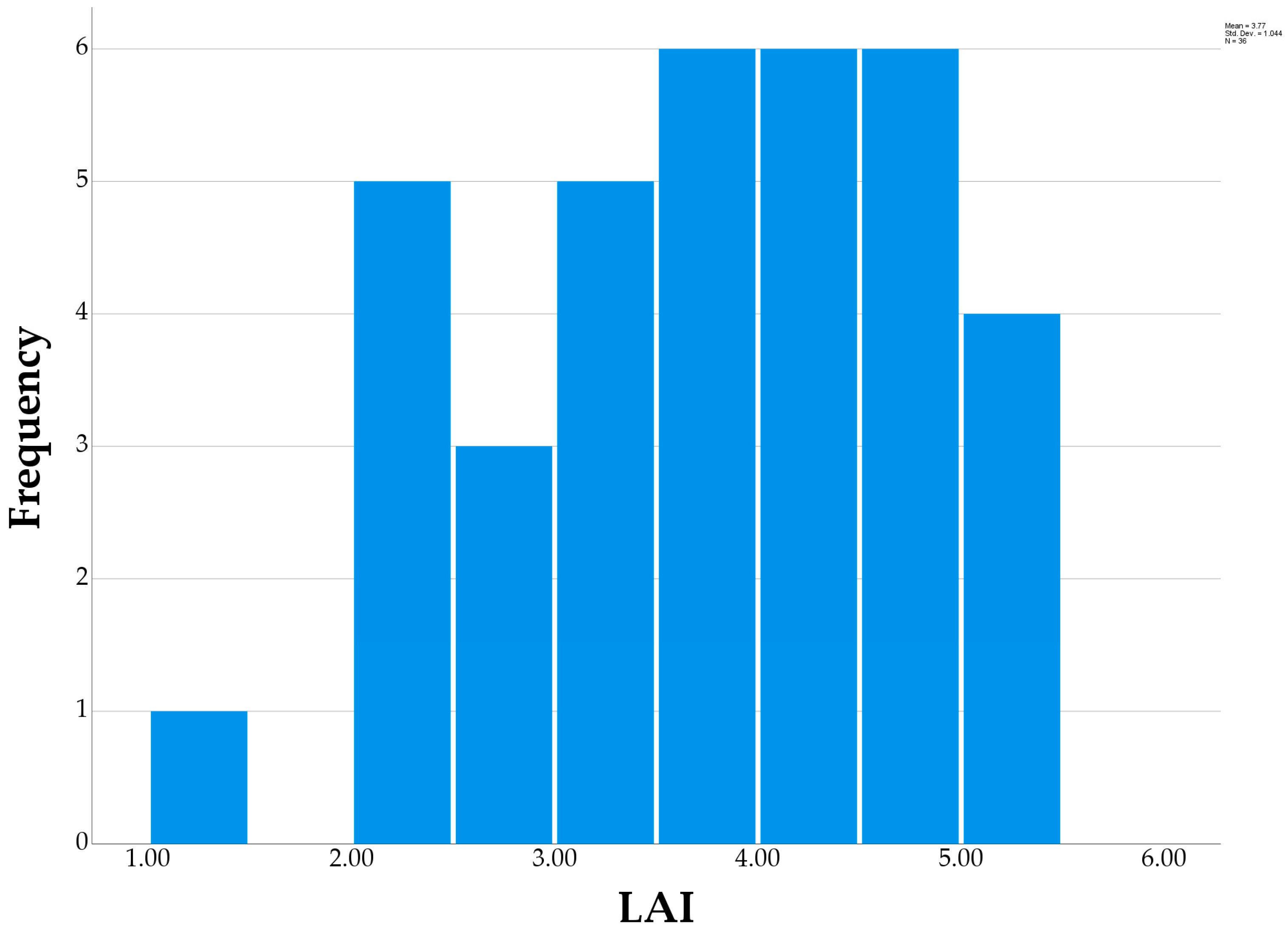
The measured LAI values displayed considerable variation, with a range of 4.09. The minimum, maximum, and mean LAI values were determined to be 1.33, 5.42, and 3.77, respectively, which aligns with the expected range of LAI from the literature for this study area. It is evident from Figure 3 that most of the plots exhibit LAI values between 3 and 5, while only one plot has an LAI value below 2.
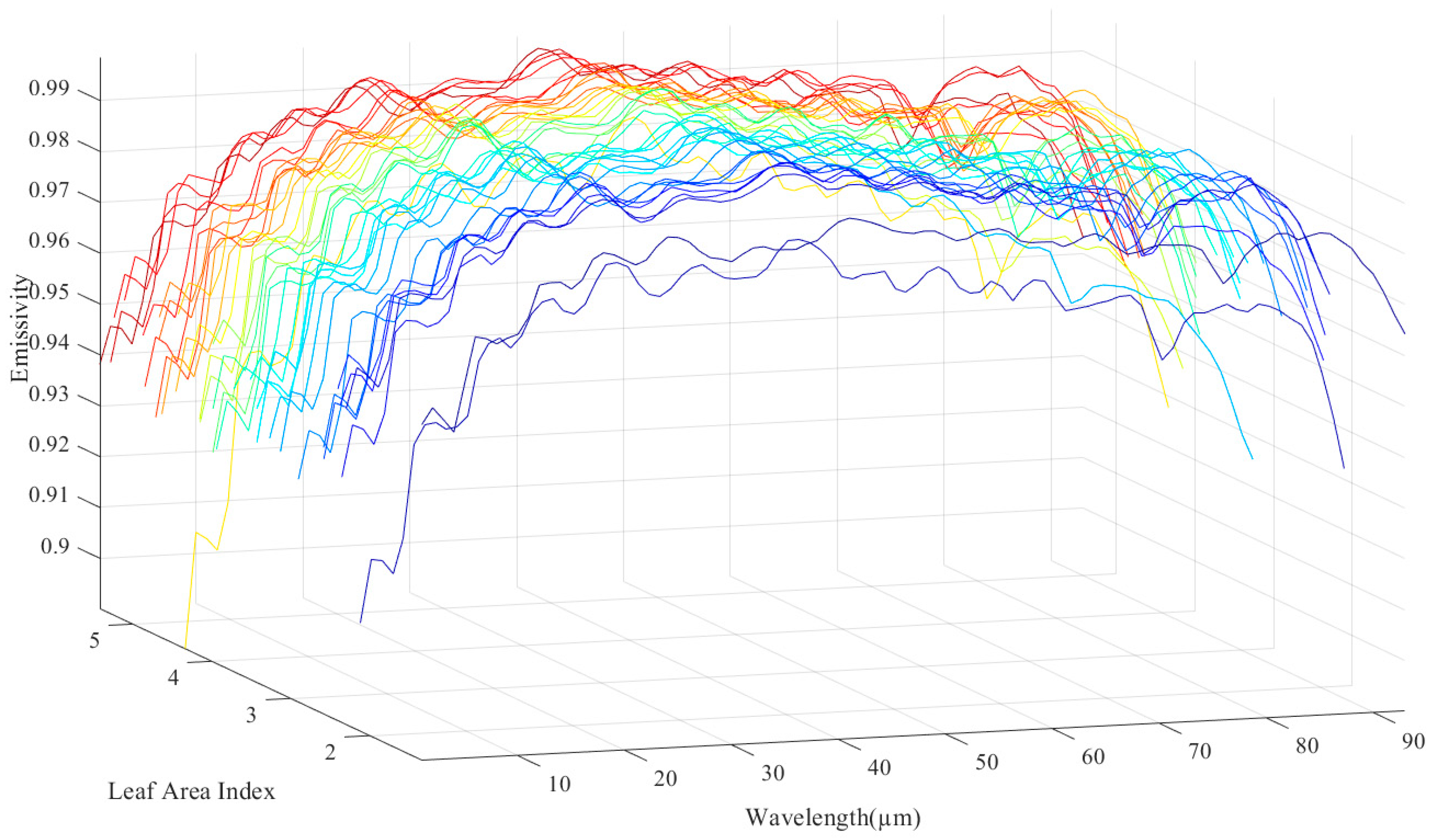
The emissivity was computed and is demonstrated in Figure 4; values extracted from each plot are depicted in Figure 5. It is evident that the extracted emissivity spectra are in agreement with the typical emissivity spectra expected for vegetation cover [27] across wavelengths ranging from 8 µm to 12.3 µm. The extracted emissivity values predominantly range from 0.94 to 0.99 µm across most plots. Nevertheless, it is noteworthy that the emissivity values are slightly lower for two plots, commencing at 0.89 at 8 µm, which are associated with relatively lower LAI values.

3.1. Narrowband Indices for Leaf Area Index Estimation

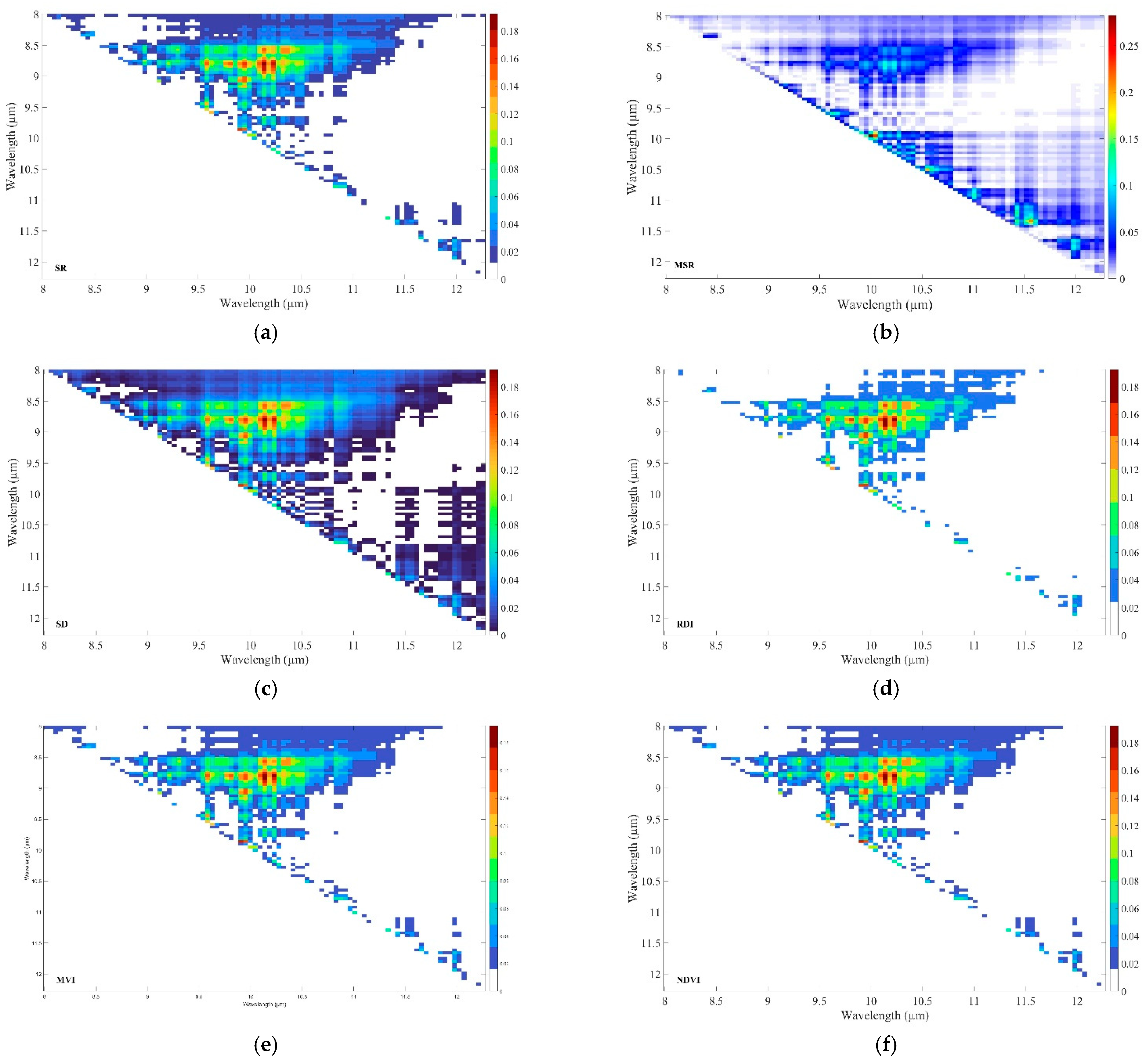
The results revealed that LAI could be retrieved with very low prediction accuracy using airborne TIR hyperspectral data, and none of the applied indices were able to successfully predict LAI (Table 2). Among the proposed indices, the MSR showed a slight ability to predict LAI (R2 = 0.28). However, the prediction accuracy for the remaining indices was surprisingly similar and low.
Figure 6 illustrates these results in a 2-D correlation plot, where each intersection of waveband pairs represents the R2 value between LAI and the spectral indices calculated using those two wavebands. The results identified wavebands including 8.75 µm, 8.79 µm, 9.95 µm, 9.99 µm, and 10.13 µm as important for LAI retrieval.

3.2. Estimation of Leaf Area Index Using Partial Least Squares Regression

The PLSR model was configured with eight factors, achieving an R2 of 0.865 and RMSECV of 0.361 (Figure 7). Figure 8 illustrates the key wavebands for LAI retrieval, as determined by the β coefficient, and Table 3 outlines their associations with vegetation biochemical components. The important wavebands for LAI retrieval identified in this study were compared with the results of Neinavaz et al. [57]. Our findings identified four critical wavebands at 8.1 µm, 9.1 µm, and within the ranges 9.85–9.95 µm and 9.99–10.27 µm, which align with those identified by Neinavaz et al. [57] in the same spectral region. However, the other wavebands (i.e., 8.01, 8.06, 8.15, 8.19, 9.35–9.62, 10.31–10.96, 11.10, 11.19, 12.210, and 12.256) were not identified or aligned with the findings of Neinavaz et al. [57].

3.3. Retrieval of Leaf Area Index Using an Artificial Neural Network

LAI could be retrieved with moderate accuracy using the LM algorithm (R2 = 0.564, RMSECV = 0.712), while the SCG algorithm predicts LAI with higher accuracy (R2 = 0.831, RMSECV = 0.184). Figure 9a shows a noticeable overestimation of LAI values between 2 and 2.5.

4. Discussion

This study assessed whether TIR hyperspectral data with high spatial resolution can accurately predict LAI in temperate forests. We found that narrowband VIs derived from emissivity spectra combinations cannot accurately predict LAI. While Neinavaz et al. [57] demonstrated that LAI could be retrieved with moderate accuracy using TIR hyperspectral data for specific species under controlled laboratory conditions, accuracy significantly decreased when emissivity spectra were pooled from different species. This aligns with our findings in the mixed temperate forest ecosystem, regardless of forest stand type. Previous studies on vegetation using TIR-RS data have highlighted the species-specific nature of TIR-RS for vegetation [25,73].
Prior research has shown that leaves of varying ages and under different illumination conditions may exhibit distinct physiological and biochemical states, resulting in different spectral emissivity and emitted TIR radiation [74]. The retrieval accuracy of LAI in this study may be influenced by ecological variables such as stand age and species composition, as these factors affect canopy structure and spectral properties. The BFNP contains diverse stand types and age classes; however, the limited number of pure plots for each type in the dataset precluded a separate statistical analysis of these variables. In addition, since this study was conducted at the canopy level in a forest, variations in vegetation species may influence heat absorption and emittance, thereby affecting species-specific TIR signatures and reducing LAI prediction accuracy. Additionally, variations in leaf physiology, such as cuticle thickness and surface texture, can affect heat absorption and radiation, influencing the accuracy of TIR-based measurements for specific species. Recently, it was revealed that leaves’ emissivity value declines from 0.99 to a minimum of 0.095 as they mature [75]. BFNP is a mixed temperate forest with diverse stands and age classes, so as mentioned before, these factors may reduce LAI prediction accuracy. While the species-specific nature of TIR data may be a disadvantage, it can aid LAI estimation in ecosystems with homogeneous vegetation. Rock et al. [76] noted that the species-specific nature of TIR data helps distinguish plant species, but success depends on the signal-to-noise ratio.
Furthermore, as observation distances increase, scale effects like mixed pixels, scattering, re-radiation, and cavity effects become more pronounced [77]. These phenomena may lead to nonlinear spectral mixtures and reduced spectral contrast [23]. Water content in vegetation is a key factor influencing TIR emission. Species differ in water storage and leaf water content, which can significantly affect their TIR signatures, resulting in distinct thermal profiles for each species [78]. The TIR response of a vegetation canopy is not just a direct measurement of foliage temperature but results from multiple factors, including canopy structure and the vertical distribution of foliage surface temperatures. The distribution of surface temperature within the foliage is influenced by a complex interplay of energy transfers, many of which are closely related to the canopy’s geometric structure [79]. Foliage density within the canopy can significantly affect the TIR signature. Variations in canopy architecture and leaf density alter heat transfer and emission processes, making it challenging to generalize TIR measurements across species [80].
The identification of key TIR wavebands, particularly around 8.1 µm, represents a significant finding in this study, highlighting spectral regions that are strongly associated with LAI using emissivity spectra. Despite a thorough review of the existing literature, we could not find explicit biochemical or biophysical mechanisms directly linking this waveband to LAI, indicating that the underlying processes remain poorly understood. It is plausible that the observed spectral relationships arise from indirect associations with canopy structural and physiological properties, including leaf emissivity, water content, and temperature, all of which can influence radiative characteristics in the TIR region. These factors likely mediate the relationship between the identified wavebands and canopy leaf area. Understanding the precise mechanistic basis would require controlled experiments linking leaf- and canopy-level traits to spectral emissivity in the TIR range.
Our findings showed that PLSR can retrieve LAI with high accuracy, even outperforming the ANN approach using the LM algorithm. This may be due to PLSR’s effectiveness with datasets with high multicollinearity among predictor variables, a common issue in spectroscopy and scientific analyses. PLSR handles this by reducing the data to a lower-dimensional space while preserving key variance for accurate predictions, making it more robust in situations where an ANN may struggle. Additionally, PLSR is a linear model [81], which makes it well-suited for cases where the relationship between variables is predominantly linear, as is the case between LAI and emissivity spectra. Previously, Neinavaz et al. [27] revealed that the relationship between LAI and emissivity spectra is linear under controlled conditions when all the noises are eliminated.
In such situations, PLSR can directly capture the underlying patterns, often leading to more accurate predictions than ANN’s complex, nonlinear approach. It is also important to emphasize that PLSR aims to maximize the covariance between predictor and response variables, effectively filtering out noise. PLSR can achieve higher accuracy than ANN by concentrating on the most relevant variance [82], particularly in datasets with a low signal-to-noise ratio. In contrast, ANN may inadvertently model the noise, resulting in less precise predictions [83]. The improvement in LAI prediction accuracy using the ANN approach can be considered significant, particularly given the choice of training algorithms. The results indicate significant differences in prediction accuracy attributable to the selection of algorithms. The SCG algorithm retrieved LAI with relatively higher accuracy compared to the LM algorithm. The LM algorithm combines the rapid convergence properties of the Gauss–Newton method with the stability of gradient descent, making it particularly effective for small- to medium-sized networks and problems with highly nonlinear relationships, such as mapping emissivity spectra to LAI. LM typically converges faster and with higher precision because it uses second-order derivative information to adjust network weights, which reduces sensitivity to local minima. In contrast, the SCG algorithm is a first-order optimization method that does not require computation of the Hessian matrix, making it more memory-efficient and suitable for larger networks. However, SCG often requires more iterations to converge and can be slower in reaching an optimal solution, particularly in cases with strongly correlated inputs or highly nonlinear relationships.
Our results revealed that there are four important wavebands, including 8.1 µm, whose association with biochemical properties in vegetation remains unknown; 9.1 µm is associated with silica and sulphate anions [24,70], and the ranges 9.85–9.95 µm and 9.99–10.27 µm are associated with Oleanolic acid [24], which are considered significant in retrieval of the LAI and coincide with those important bands identified by Neinavaz et al. [57] under controlled laboratory conditions.

5. Conclusions

This research focused on estimating LAI using airborne TIR hyperspectral data by applying narrowband VIs, PLSR, and ANN. Our findings indicate that the success of TIR hyperspectral data in retrieving LAI is relatively limited, and the accuracy of the predictions is highly sensitive to the choice of the retrieval approach. While each approach offers unique strengths, their performance is notably influenced by various factors inherent in the data. PLSR, for instance, excels at managing noise due to its ability to capture relevant variance, whereas ANN may be overfit with noise, leading to less reliable predictions.
Furthermore, this research underscores the need for further investigation into other contributing factors, particularly the impact of stand age and species composition on LAI retrieval using TIR hyperspectral data. Differences in vegetation characteristics could alter the spectral response, affecting the robustness and accuracy of the LAI retrieval methods.
Future research should therefore (1) systematically evaluate the influence of stand age and species composition on TIR-based LAI retrieval and (2) explore hybrid or ensemble modelling approaches that integrate the strengths of both regression-based and machine learning methods. Such targeted efforts will be essential for enhancing the robustness and accuracy of LAI estimates in future TIR remote sensing applications.

Author Contributions

Conceptualization, E.N., R.D. and A.K.S.; methodology, E.N.; software, E.N.; validation, E.N.; formal analysis, E.N.; investigation, E.N.; resources, A.K.S. and M.H.; data curation, E.N.; writing—original draft preparation, E.N.; writing—review and editing, E.N., R.D., A.K.S., M.H. and X.Z.; visualization, E.N.; supervision, E.N.; project administration, R.D., A.K.S. and M.H.; funding acquisition, A.K.S. All authors have read and agreed to the published version of the manuscript.

Funding

This research received financial support from the Department of Natural Resources, Faculty of Geo-Information Science and Earth Observation (ITC), University of Twente, and was co-funded by BFNP. Skidmore was supported by the European Research Council (ERC) through the EU-Horizon 2020 research and innovation program, grant agreement n° 834709. Funding was also provided by the European Facility for Airborne Research in Environmental and Geo-sciences (EUFAR) under the EC’s 7th Framework Programme (FP7/2014-2018), grant agreement n° 312609.

Data Availability Statement

Airborne data is available upon submitting a request to EUFAR. All users must acknowledge the data providers in any publication based on EUFAR data.

Acknowledgments

The authors thank Stefanie Holzwarth, Ils Reusen, and Tawanda Gara for their assistance during the EUFAR field and flight campaigns and appreciate the support from the BFNP management, Bavarian State Forest Enterprise (Bayerische Staatsforsten), Neuburg Forest, and the Bavarian Forest’s Data Pool initiative for the Bohemian Forest Ecosystem.

Conflicts of Interest

All the authors confirm that no known conflicts of interest are associated with this publication, and all authors have approved the manuscript.

Abbreviations

The following abbreviations are used in this manuscript:
ANNArtificial Neural Network
BFNPBavarian Forest National Park
ITCFaculty of Geo-Information Science and Earth Observation
LAILeaf Area Index
LMLevenberg–Marquardt
PLSRPartial Least Squares Regression
R2Coefficients of Determination
RMSERoot Mean Squared Error
RMSECVCross-Validation Root Mean Squared Error
RSRemote Sensing
SCGScaled Conjugate Gradient
TIRThermal infrared
UAVUnmanned Aerial Vehicle
VIsVegetation Indices
VIS-SWIRVisible-Short Wave Infrared

References

  1. Fang, H.; Baret, F.; Plummer, S.; SchaepmanÔÇÉStrub, G. An overview of global leaf area index (LAI): Methods, products, validation, and applications. Rev. Geophys. 2019, 57, 739–799. [Google Scholar] [CrossRef]
  2. Tripathi, A.M.; Pohanková, E.; Fischer, M.; Orság, M.; Trnka, M.; Klem, K.; Marek, M.V. The evaluation of radiation use efficiency and leaf area index development for the estimation of biomass accumulation in short rotation poplar and annual field crops. Forests 2018, 9, 168. [Google Scholar] [CrossRef]
  3. Taugourdeau, S.; Le Maire, G.; Avelino, J.; Jones, J.R.; Ramirez, L.G.; Quesada, M.J.; Charbonnier, F.; Gómez-Delgado, F.; Harmand, J.-M.; Rapidel, B. Leaf area index as an indicator of ecosystem services and management practices: An application for coffee agroforestry. Agric. Ecosyst. Environ. 2014, 192, 19–37. [Google Scholar] [CrossRef]
  4. Bojinski, S.; Verstraete, M.; Peterson, T.C.; Richter, C.; Simmons, A.; Zemp, M. The concept of essential climate variables in support of climate research, applications, and policy. Bull. Am. Meteorol. Soc. 2014, 95, 1431–1443. [Google Scholar] [CrossRef]
  5. Skidmore, A.K.; Coops, N.C.; Neinavaz, E.; Ali, A.; Schaepman, M.E.; Paganini, M.; Kissling, W.D.; Vihervaara, P.; Darvishzadeh, R.; Feilhauer, H.; et al. Priority list of biodiversity metrics to observe from space. Nat. Ecol. Evol. 2021, 5, 896–906. [Google Scholar] [CrossRef]
  6. Skidmore, A.K.; Pettorelli, N.; Coops, N.C.; Geller, G.N.; Hansen, M.; Lucas, R.; Mücher, C.A.; O’Connor, B.; Paganini, M.; Pereira, H.M.; et al. Environmental science: Agree on biodiversity metrics to track from space. Nature 2015, 523, 403–405. [Google Scholar] [CrossRef] [PubMed]
  7. Clevers, J.G.; Kooistra, L.; Schaepman, M.E. Estimating canopy water content using hyperspectral remote sensing data. Int. J. Appl. Earth Obs. Geoinf. 2010, 12, 119–125. [Google Scholar] [CrossRef]
  8. Hunt, E.R., Jr.; Wang, L.; Qu, J.J.; Hao, X. Remote sensing of fuel moisture content from canopy water indices and normalized dry matter index. J. Appl. Remote Sens. 2012, 6, 061705. [Google Scholar] [CrossRef]
  9. Yebra, M.; Dennison, P.E.; Chuvieco, E.; Riaño, D.; Zylstra, P.; Hunt, E.R., Jr.; Danson, F.M.; Qi, Y.; Jurdao, S. A global review of remote sensing of live fuel moisture content for fire danger assessment: Moving towards operational products. Remote Sens. Environ. 2013, 136, 455–468. [Google Scholar] [CrossRef]
  10. Simic, A.; Fernandes, R.; Wang, S. Assessing the impact of leaf area index on evapotranspiration and groundwater recharge across a shallow water region for diverse land cover and soil properties. J. Water Resour. Hydraul. Eng 2014, 3, 60–73. [Google Scholar]
  11. Liu, Y.; Xiao, J.; Ju, W.; Zhu, G.; Wu, X.; Fan, W.; Li, D.; Zhou, Y. Satellite-derived LAI products exhibit large discrepancies and can lead to substantial uncertainty in simulated carbon and water fluxes. Remote Sens. Environ. 2018, 206, 174–188. [Google Scholar] [CrossRef]
  12. Kang, Y.; Ozdogan, M.; Gao, F.; Anderson, M.C.; White, W.A.; Yang, Y.; Yang, Y.; Erickson, T.A. A data-driven approach to estimate leaf area index for Landsat images over the contiguous US. Remote Sens. Environ. 2021, 258, 112383. [Google Scholar] [CrossRef]
  13. Pu, R.; Landry, S. Evaluating seasonal effect on forest leaf area index mapping using multi-seasonal high resolution satellite pléiades imagery. Int. J. Appl. Earth Obs. Geoinf. 2019, 80, 268–279. [Google Scholar] [CrossRef]
  14. Tillack, A.; Clasen, A.; Kleinschmit, B.; Förster, M. Estimation of the seasonal leaf area index in an alluvial forest using high-resolution satellite-based vegetation indices. Remote Sens. Environ. 2014, 141, 52–63. [Google Scholar] [CrossRef]
  15. Xie, R.; Darvishzadeh, R.; Skidmore, A.K.; Heurich, M.; Holzwarth, S.; Gara, T.W.; Reusen, I. Mapping leaf area index in a mixed temperate forest using Fenix airborne hyperspectral data and Gaussian processes regression. Int. J. Appl. Earth Obs. Geoinf. 2021, 95, 102242. [Google Scholar] [CrossRef]
  16. Xie, Q.; Huang, W.; Liang, D.; Chen, P.; Wu, C.; Yang, G.; Zhang, J.; Huang, L.; Zhang, D. Leaf area index estimation using vegetation indices derived from airborne hyperspectral images in winter wheat. IEEE J. Sel. Top. Appl. Earth Obs. Remote Sens. 2014, 7, 3586–3594. [Google Scholar] [CrossRef]
  17. Qi, H.; Zhu, B.; Wu, Z.; Liang, Y.; Li, J.; Wang, L.; Chen, T.; Lan, Y.; Zhang, L. Estimation of peanut leaf area index from unmanned aerial vehicle multispectral images. Sensors 2020, 20, 6732. [Google Scholar] [CrossRef] [PubMed]
  18. Stobbelaar, P.; Neinavaz, E.; Nyktas, P. Prediction of leaf area index using thermal infrared data acquired by UAS over a mixed temperate forest. Int. J. Appl. Earth Obs. Geoinf. 2022, 114, 103049. [Google Scholar] [CrossRef]
  19. Delegido, J.; Verrelst, J.; Alonso, L.; Moreno, J. Evaluation of sentinel-2 red-edge bands for empirical estimation of green LAI and chlorophyll content. Sensors 2011, 11, 7063–7081. [Google Scholar] [CrossRef]
  20. Atzberger, C.; Richter, K. Spatially constrained inversion of radiative transfer models for improved LAI mapping from future Sentinel-2 imagery. Remote Sens. Environ. 2012, 120, 208–218. [Google Scholar] [CrossRef]
  21. Laurent, V.C.; Schaepman, M.E.; Verhoef, W.; Weyermann, J.; Chávez, R.O. Bayesian object-based estimation of LAI and chlorophyll from a simulated Sentinel-2 top-of-atmosphere radiance image. Remote Sens. Environ. 2014, 140, 318–329. [Google Scholar] [CrossRef]
  22. Verrelst, J.; Rivera, J.P.; Veroustraete, F.; Muñoz-Marí, J.; Clevers, J.G.; Camps-Valls, G.; Moreno, J. Experimental Sentinel-2 LAI estimation using parametric, non-parametric and physical retrieval methods–A comparison. ISPRS J. Photogramm. Remote Sens. 2015, 108, 260–272. [Google Scholar] [CrossRef]
  23. Ribeiro da Luz, B.; Crowley, J.K. Identification of plant species by using high spatial and spectral resolution thermal infrared (8.0–13.5 μm) imagery. Remote Sens. Environ. 2010, 114, 404–413. [Google Scholar] [CrossRef]
  24. Ribeiro da Luz, B.; Crowley, J.K. Spectral reflectance and emissivity features of broad leaf plants: Prospects for remote sensing in the thermal infrared (8.0–14.0 μm). Remote Sens. Environ. 2007, 109, 393–405. [Google Scholar] [CrossRef]
  25. Neinavaz, E.; Schlerf, M.; Darvishzadeh, R.; Gerhards, M.; Skidmore, A.K. Thermal infrared remote sensing of vegetation: Current status and perspectives. Int. J. Appl. Earth Obs. Geoinf. 2021, 102, 102415. [Google Scholar] [CrossRef]
  26. Neinavaz, E.; Darvishzadeh, R.; Skidmore, A.K.; Abdullah, H. Integration of Landsat-8 Thermal and Visible-Short Wave Infrared Data for Improving Prediction Accuracy of Forest Leaf Area Index. Remote Sens. 2019, 11, 390. [Google Scholar] [CrossRef]
  27. Neinavaz, E.; Darvishzadeh, R.; Skidmore, A.K.; Groen, T.A. Measuring the response of canopy emissivity spectra to leaf area index variation using thermal hyperspectral data. Int. J. Appl. Earth Obs. Geoinf. 2016, 53, 40–47. [Google Scholar] [CrossRef]
  28. Heurich, M.; Beudert, B.; Rall, H.; Křenová, Z. Long-Term Ecological Research; Springer: Berlin/Heidelberg, Germany, 2010; pp. 327–344. [Google Scholar]
  29. Huber, C. Long lasting nitrate leaching after bark beetle attack in the highlands of the Bavarian Forest National Park. J. Environ. Qual. 2005, 34, 1772–1779. [Google Scholar] [CrossRef] [PubMed]
  30. Gara, T.W.; Darvishzadeh, R.; Skidmore, A.K.; Wang, T.; Heurich, M. Accurate modelling of canopy traits from seasonal Sentinel-2 imagery based on the vertical distribution of leaf traits. ISPRS J. Photogramm. Remote Sens. 2019, 157, 108–123. [Google Scholar] [CrossRef]
  31. Silveyra Gonzalez, R.; Latifi, H.; Weinacker, H.; Dees, M.; Koch, B.; Heurich, M. Integrating LiDAR and high-resolution imagery for object-based mapping of forest habitats in a heterogeneous temperate forest landscape. Int. J. Remote Sens. 2018, 39, 8859–8884. [Google Scholar] [CrossRef]
  32. Darvishzadeh, R.; Skidmore, A.; Schlerf, M.; Atzberger, C. Inversion of a radiative transfer model for estimating vegetation LAI and chlorophyll in a heterogeneous grassland. Remote Sens. Environ. 2008, 112, 2592–2604. [Google Scholar] [CrossRef]
  33. Liu, C.; Xu, R.; Xie, F.; Jin, J.; Yuan, L.; Lv, G.; Wang, Y.; Li, C.; Wang, J. New airborne thermal-infrared hyperspectral imager system: Initial validation. IEEE J. Sel. Top. Appl. Earth Obs. Remote Sens. 2020, 13, 4149–4165. [Google Scholar] [CrossRef]
  34. Harris, L.; Warren, M.; Grant, M.; Llewellyn, G.M. Spectral characterization of the AisaOWL. IEEE Trans. Geosci. Remote Sens. 2017, 55, 2751–2756. [Google Scholar] [CrossRef]
  35. Harris, L.J.; Warren, M.; Clewley, D.; Taylor, B.; Llewellyn, G.; Maclellan, C.; Mata, A.; Goult, S.; Grant, M.; Groom, S. NERC-ARSF-DAN Thermal Hyperspectral Data Quality Report 2015, 2016.
  36. Wolosin, M.; Harris, N. Tropical Forests and Climate Change: The Latest Science; World Resources Institute: Washington, DC, USA, 2018. [Google Scholar]
  37. Manolakis, D.; Pieper, M.; Truslow, E.; Lockwood, R.; Weisner, A.; Jacobson, J.; Cooley, T. Longwave infrared hyperspectral imaging: Principles, progress, and challenges. IEEE Geosci. Remote Sens. Mag. 2019, 7, 72–100. [Google Scholar] [CrossRef]
  38. Minkina, W.; Dudzik, S. Infrared Thermography: Errors and Uncertainties; John Wiley & Sons: Hoboken, NJ, USA, 2009. [Google Scholar]
  39. Vollmer, M. Computer Vision: A Reference Guide; Springer: Berlin/Heidelberg, Germany, 2020; pp. 1–4. [Google Scholar]
  40. Borel, C.C. Iterative Retrieval of Surface Emissivity and Temperature for a Hyperspectral Sensor; Los Alamos National Lab. (LANL): Los Alamos, NM, USA, 1997. [Google Scholar]
  41. Realmuto, V. Separating the effects of temperature amd emissivity: Emissivity spectrum normalization. In Proceedings of the Second Thermal Infrared Multispectral Scanner (TIMS) Workshop, Reston, Virginia, 29–30 October 1985; pp. 31–35. [Google Scholar]
  42. Young, S.J.; Johnson, B.R.; Hackwell, J.A. An in-scene method for atmospheric compensation of thermal hyperspectral data. J. Geophys. Res. Atmos. 2002, 107, 4774. [Google Scholar] [CrossRef]
  43. Norman, J.M.; Divakarla, M.; Goel, N.S. Algorithms for extracting information from remote thermal-IR observations of the earth’s surface. Remote Sens. Environ. 1995, 51, 157–168. [Google Scholar] [CrossRef]
  44. Norman, J.M.; Becker, F. Terminology in thermal infrared remote sensing of natural surfaces. Agric. For. Meteorol. 1995, 77, 153–166. [Google Scholar] [CrossRef]
  45. Savitzky, A.; Golay, M.J. Smoothing and differentiation of data by simplified least squares procedures. Anal. Chem. 1964, 36, 1627–1639. [Google Scholar] [CrossRef]
  46. Darvishzadeh, R.; Atzberger, C.; Skidmore, A.; Schlerf, M. Mapping grassland leaf area index with airborne hyperspectral imagery: A comparison study of statistical approaches and inversion of radiative transfer models. ISPRS J. Photogramm. Remote Sens. 2011, 66, 894–906. [Google Scholar] [CrossRef]
  47. Huete, A.; Didan, K.; Miura, T.; Rodriguez, E.P.; Gao, X.; Ferreira, L.G. Overview of the radiometric and biophysical performance of the MODIS vegetation indices. Remote Sens. Environ. 2002, 83, 195–213. [Google Scholar] [CrossRef]
  48. Chen, J.M.; Cihlar, J. Retrieving leaf area index of boreal conifer forests using Landsat TM images. Remote Sens. Environ. 1996, 55, 153–162. [Google Scholar] [CrossRef]
  49. Viña, A.; Bearer, S.; Zhang, H.; Ouyang, Z.; Liu, J. Evaluating MODIS data for mapping wildlife habitat distribution. Remote Sens. Environ. 2008, 112, 2160–2169. [Google Scholar] [CrossRef]
  50. Jordan, C.F. Derivation of leaf area index from quality of light on the forest floor. Ecology 1969, 50, 663–666. [Google Scholar] [CrossRef]
  51. Chen, J.M. Evaluation of vegetation indices and a modified simple ratio for boreal applications. Can. J. Remote Sens. 1996, 22, 229–242. [Google Scholar] [CrossRef]
  52. Tucker, C.J. Red and photographic infrared linear combinations for monitoring vegetation. Remote Sens. Environ. 1979, 8, 127–150. [Google Scholar] [CrossRef]
  53. Roujean, J.-L.; Breon, F.-M. Estimating PAR absorbed by vegetation from bidirectional reflectance measurements. Remote Sens. Environ. 1995, 51, 375–384. [Google Scholar] [CrossRef]
  54. Paltridge, G.; Barber, J. Monitoring grassland dryness and fire potential in Australia with NOAA/AVHRR data. Remote Sens. Environ. 1988, 25, 381–394. [Google Scholar] [CrossRef]
  55. Rouse, J.; Haas, R.; Schell, J.; Deering, D.; Harlan, J. Monitoring the Vernal Advancements and Retrogradation of Natural Vegetation; NASA/GSFC Final Report; NASA: Greenbelt MD USA, 1974; pp. 1–137. [Google Scholar]
  56. Cho, M.A.; Skidmore, A.; Corsi, F.; Van Wieren, S.E.; Sobhan, I. Estimation of green grass/herb biomass from airborne hyperspectral imagery using spectral indices and partial least squares regression. Int. J. Appl. Earth Obs. Geoinf. 2007, 9, 414–424. [Google Scholar] [CrossRef]
  57. Neinavaz, E.; Skidmore, A.K.; Darvishzadeh, R.; Groen, T.A. Retrieval of leaf area index in different plant species using thermal hyperspectral data. ISPRS J. Photogramm. Remote Sens. 2016, 119, 390–401. [Google Scholar] [CrossRef]
  58. Duda, R.O.; Hart, P.E. Pattern classification and scene analysis. A Wiley-Interscience Publication; Wiley: New York, NY, USA, 1973. [Google Scholar]
  59. Geladi, P.; Kowalski, B.R. Partial least-squares regression: A tutorial. Anal. Chim. Acta 1986, 185, 1–17. [Google Scholar] [CrossRef]
  60. Haaland, D.M.; Thomas, E.V. Partial least-squares methods for spectral analyses. 1. Relation to other quantitative calibration methods and the extraction of qualitative information. Anal. Chem. 1988, 60, 1193–1202. [Google Scholar] [CrossRef]
  61. Chai, L.; Qu, Y.; Zhang, L.; Liang, S.; Wang, J. Estimating time-series leaf area index based on recurrent nonlinear autoregressive neural networks with exogenous inputs. Int. J. Remote Sens. 2012, 33, 5712–5731. [Google Scholar] [CrossRef]
  62. Johnson, D.M.; Smith, W.K.; Vogelmann, T.C.; Brodersen, C.R. Leaf architecture and direction of incident light influence mesophyll fluorescence profiles. Am. J. Bot. 2005, 92, 1425–1431. [Google Scholar] [CrossRef]
  63. Wu, T.; Zhang, Z.; Wang, Q.; Jin, W.; Meng, K.; Wang, C.; Yin, G.; Xu, B.; Shi, Z. Estimating rice leaf area index at multiple growth stages with Sentinel-2 data: An evaluation of different retrieval algorithms. Eur. J. Agron. 2024, 161, 127362. [Google Scholar] [CrossRef]
  64. Wang, T.; Xiao, Z.; Liu, Z. Performance evaluation of machine learning methods for leaf area index retrieval from time-series MODIS reflectance data. Sensors 2017, 17, 81. [Google Scholar] [CrossRef] [PubMed]
  65. Atkinson, P.M.; Tatnall, A.R. Introduction neural networks in remote sensing. Int. J. Remote Sens. 1997, 18, 699–709. [Google Scholar] [CrossRef]
  66. Nowlan, S.J.; Hinton, G.E. Simplifying neural networks by soft weight-sharing. Neural Comput. 1992, 4, 473–493. [Google Scholar] [CrossRef]
  67. Boeriu, C.G.; Bravo, D.; Gosselink, R.J.; van Dam, J.E. Characterisation of structure-dependent functional properties of lignin with infrared spectroscopy. Ind. Crops Prod. 2004, 20, 205–218. [Google Scholar] [CrossRef]
  68. Socrates, G. Infrared and Raman Characteristic Group Frequencies: Tables and Charts; John Wiley & Sons: Hoboken, NJ, USA, 2004. [Google Scholar]
  69. Elvidge, C.D. Thermal infrared reflectance of dry plant materials: 2.5–20.0 μm. Remote Sens. Environ. 1988, 26, 265–285. [Google Scholar] [CrossRef]
  70. Mayo, D.W.; Miller, F.A.; Hannah, R.W. Course Notes on the Interpretation of Infrared and Raman Spectra; John Wiley & Sons: Hoboken, NJ, USA, 2004. [Google Scholar]
  71. Ribeiro da Luz, B. Attenuated total reflectance spectroscopy of plant leaves: A tool for ecological and botanical studies. New Phytol. 2006, 172, 305–318. [Google Scholar] [CrossRef]
  72. Stewart, D.; Yahiaoui, N.; McDougall, G.J.; Myton, K.; Marque, C.ę.; Boudet, A.M.; Haigh, J. Fourier-transform infrared and Raman spectroscopic evidence for the incorporation of cinnamaldehydes into the lignin of transgenic tobacco (Nicotiana tabacum L.) plants with reduced expression of cinnamyl alcohol dehydrogenase. Planta 1997, 201, 311–318. [Google Scholar] [CrossRef]
  73. Ullah, S.; Skidmore, A.K.; Naeem, M.; Schlerf, M. An accurate retrieval of leaf water content from mid to thermal infrared spectra using continuous wavelet analysis. Sci. Total Environ. 2012, 437, 145–152. [Google Scholar] [CrossRef] [PubMed]
  74. Buitrago, M.F.; Groen, T.A.; Hecker, C.A.; Skidmore, A.K. Changes in thermal infrared spectra of plants caused by temperature and water stress. ISPRS J. Photogramm. Remote Sens. 2016, 111, 22–31. [Google Scholar] [CrossRef]
  75. Richardson, A.D.; Aubrecht, D.M.; Basler, D.; Hufkens, K.; Muir, C.D.; Hanssen, L. Developmental changes in the reflectance spectra of temperate deciduous tree leaves and implications for thermal emissivity and leaf temperature. New Phytol. 2021, 229, 791–804. [Google Scholar] [CrossRef]
  76. Rock, G.; Gerhards, M.; Schlerf, M.; Hecker, C.; Udelhoven, T. Plant species discrimination using emissive thermal infrared imaging spectroscopy. Int. J. Appl. Earth Obs. Geoinf. 2016, 53, 16–26. [Google Scholar] [CrossRef]
  77. Kirkland, L.; Herr, K.; Keim, E.; Adams, P.; Salisbury, J.; Hackwell, J.; Treiman, A. First use of an airborne thermal infrared hyperspectral scanner for compositional mapping. Remote Sens. Environ. 2002, 80, 447–459. [Google Scholar] [CrossRef]
  78. Fabre, S.; Lesaignoux, A.; Olioso, A.; Briottet, X. Influence of Water Content on Spectral Reflectance of Leaves in the 3–15. IEEE Geosci. Remote Sens. Lett. 2011, 8, 143–147. [Google Scholar] [CrossRef]
  79. Lagouarde, J.-P.; Kerr, Y.H.; Brunet, Y. An experimental study of angular effects on surface temperature for various plant canopies and bare soils. Agric. For. Meteorol. 1995, 77, 167–190. [Google Scholar] [CrossRef]
  80. Still, C.; Powell, R.; Aubrecht, D.; Kim, Y.; Helliker, B.; Roberts, D.; Richardson, A.; Goulden, M. Thermal imaging in plant and ecosystem ecology: Applications and challenges. Ecosphere 2019, 10, e02768. [Google Scholar] [CrossRef]
  81. Cheng, J.-H.; Sun, D.-W. Partial least squares regression (PLSR) applied to NIR and HSI spectral data modeling to predict chemical properties of fish muscle. Food Eng. Rev. 2017, 9, 36–49. [Google Scholar] [CrossRef]
  82. Tran, T.N.; Afanador, N.L.; Buydens, L.M.; Blanchet, L. Interpretation of variable importance in partial least squares with significance multivariate correlation (sMC). Chemom. Intell. Lab. Syst. 2014, 138, 153–160. [Google Scholar] [CrossRef]
  83. Vega, J.; Reynoso, R.; Calvet, H.C. Effect of signal noise on the learning capability of an artificial neural network. Nucl. Instrum. Methods Phys. Res. Sect. A Accel. Spectrometers Detect. Assoc. Equip. 2009, 606, 693–699. [Google Scholar] [CrossRef]
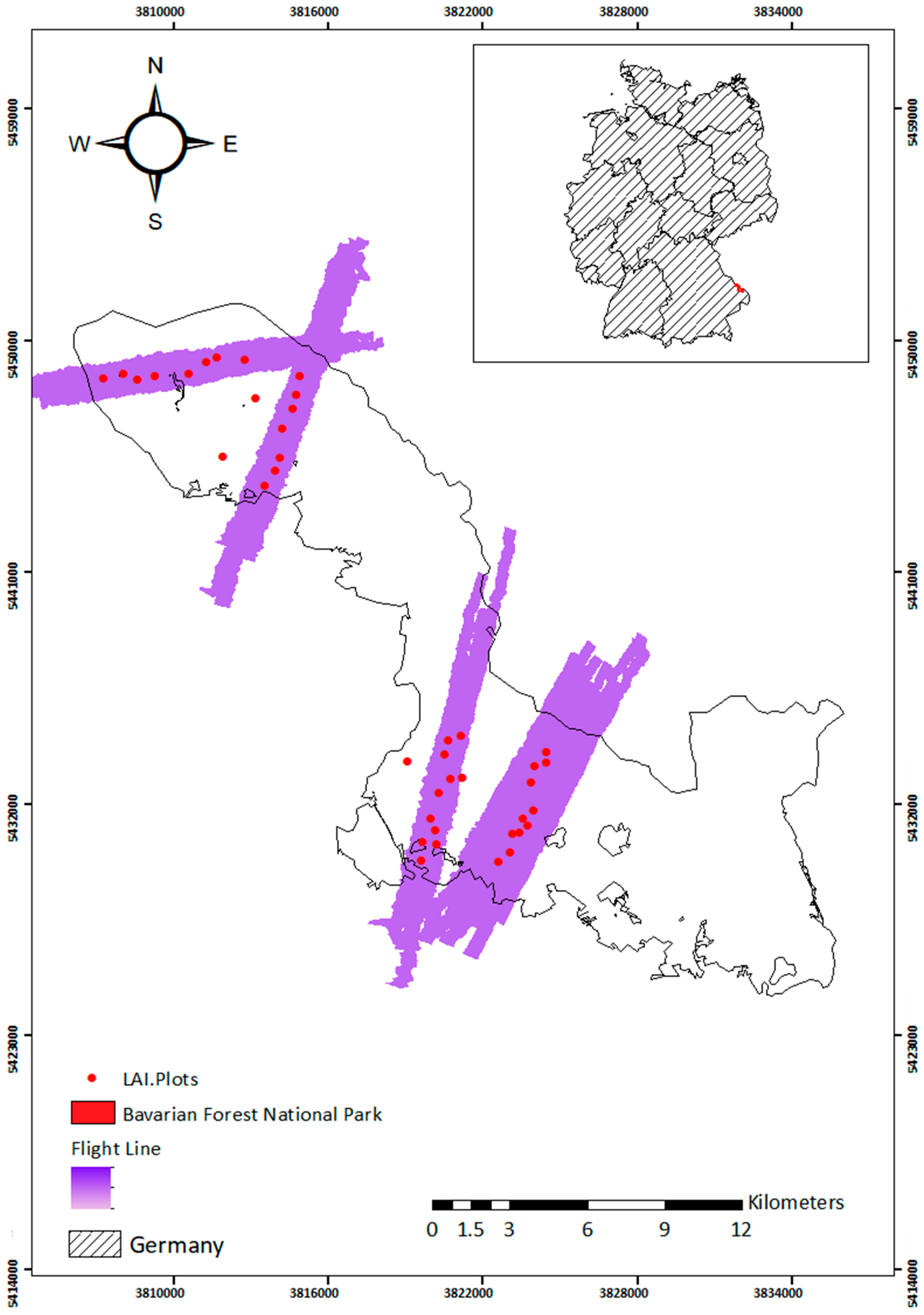
Figure 1. The location of the Bavarian Forest National Park in southeastern Germany, the plot arrangement across the study area, along with the flight lines followed during the flight campaign.
Remotesensing 17 03820 g001
Figure 3. The Leaf Area Index (LAI) histogram values are based on 36 plots.
Remotesensing 17 03820 g003
Figure 4. The emissivity spectra were computed for the Bavarian Forest National Park in Germany.
Remotesensing 17 03820 g004
Figure 5. Emissivity spectra extracted for each plot (n = 36). Colors are for visual distinction only and are not described further.
Remotesensing 17 03820 g005
Figure 6. Two-dimensional correlation plots showing the coefficient of determination between the Leaf Area Index and vegetation indices, including (a) Simple Ratio Index, (b) Modified Simple Ratio Index, (c) Difference Vegetation Index, (d) Renormalized Difference Index, (e) Modified Vegetation Index, and (f) Normalized Difference Vegetation Index. All indices were derived from every possible pair of wavebands within the 8 µm to 12.3 µm spectral range.
Remotesensing 17 03820 g006
Figure 7. A scatterplot illustrates the relationship between the measured and predicted Leaf Area Index, obtained by applying a partial least squares regression model.
Remotesensing 17 03820 g007
Figure 8. The β coefficients derived from the PLSR model for the prediction of Leaf Area Index. The significance threshold is defined based on the standard deviation of the β coefficients.
Remotesensing 17 03820 g008
Figure 9. Scatterplot showing the relationship between measured and retrieved Leaf Area Index using an artificial neural network with (a) Levenberg–Marquardt and (b) Scaled Conjugate Gradient algorithms.
Remotesensing 17 03820 g009
Table 1. Leaf Area Index derived from emissivity spectra using narrowband indices.
Vegetation IndexAcronymInitial EquationImplemented EquationReference
Simple RatioSR* ρ N I R ρ R e d ** ρ λ 1 ρ λ 2 [50]
Modified Simple RatioMSR ρ N I R     ρ R e d     1 ρ N I R / ρ R e d 0.5   +   1 ρ λ 1     ρ λ 2     1 ρ λ 1 / ρ λ 2 0.5   +   1 [51]
Difference Vegetation IndexSD ρ N I R     ρ R e d ρ λ 1     ρ λ 2 [52]
Re-normalized Difference IndexRDI ρ N I R     ρ R e d ρ N I R   +   ρ R e d ρ λ 1     ρ λ 2 ρ λ 1   +   ρ λ 2 [53]
Modified Vegetation IndexMVI ρ N I R     1.2 ρ R e d ρ N I R   +   ρ R e d ρ λ 1     1.2 ρ λ 2 ρ λ 1   +   ρ λ 2 [54]
Normalized Difference Vegetation IndexNDVI ρ N I R     ρ R e d ρ N I R   +   ρ R e d ρ λ 1     ρ λ 2 ρ λ 1   +   ρ λ 2 [55]
* ρ is the reflectance value at a given wavelength λ, and NIR is the near-infrared reflectance. ** λ1, λ2, and λ3 are canopy emissivity spectra at different wavebands.
Table 2. Use of coefficients of determination (R2) and cross-validation RMSE (RMSECV) to evaluate top-performing narrowband vegetation indices for Leaf Area Index prediction.
IndexMost Sensitive Wavebands CombinationR2RMSECV
SR9.95 µm and 9.99 µm0.190.003
MSR9.95 µm and 9.99 µm0.280.002
SD8.75 µm and 10.13 µm0.190.001
RDI8.79 µm and 10.13 µm0.190.009
MVI8.79 µm and 10.13 µm0.190.007
NDVI8.79 µm and 10.13 µm0.190.007
Table 3. Significant wavebands for Leaf Area Index retrieval identified in this study, compared with those found by Neinavaz et al. [57]. The bold numbers refer to the wavebands that were identified as significant in the current and previous study by Neinavaz et al.
Important Wavebands (µm) Associated Biochemical PropertiesReference
Neinavaz, et al. [57]Current Study
-8.01CutinRibeiro da Luz and Crowley [24]
-8.06CutinRibeiro da Luz and Crowley [24]
8.18.10--
-8.15--
-8.19LigninBoeriu, et al. [67]
8.4-LigninSocrates [68]
8.5-Cellulose, CutinRibeiro da Luz and Crowley [24]
8.8-Cellulose
9.0-Cellulose [24,69]
9.19.12Silica, Sulphate anion[24], Mayo et al. [70]
9.2-CelluloseElvidge [69]
-9.35CelluloseElvidge [69]
-9.49CelluloseRibeiro da Luz and Crowley [24]
-9.53--
-9.58--
-9.62Hemicellulose xylan Ribeiro da Luz and Crowley [24]
9.7–10.029.85–9.95Oleanolic acidRibeiro da Luz [71]
9.9–10.29.99–10.27Oleanolic acidRibeiro da Luz and Crowley [24]
-10.31–10.96Cellulose, Hollocellulose, EsterElvidge [69], Stewart et al. [72]
-11.103--
-11.195--
11.86–11.94-LigninBoeriu, et al. [67], Elvidge [69]
12.0-CutinRibeiro da Luz and Crowley [24]
12.1-CutinRibeiro da Luz and Crowley [24]
-12.210--
-12.256--
Disclaimer/Publisher’s Note: The statements, opinions and data contained in all publications are solely those of the individual author(s) and contributor(s) and not of MDPI and/or the editor(s). MDPI and/or the editor(s) disclaim responsibility for any injury to people or property resulting from any ideas, methods, instructions or products referred to in the content.