Deep Learning-Based Classification of Aquatic Vegetation Using GF-1/6 WFV and HJ-2 CCD Satellite Data

Highlights

What are the main findings?

• This study demonstrated that high-temporal-resolution Chinese satellite data—aofen-1/6 (GF-1/6) Wide Field of View (WFV) and Huanjing-2A/B (HJ-2A/B)—with 16 m spatial resolution, 1-day revisit capability after constellation networking, and consistent spectral performance, can support effective extraction of aquatic vegetation.
• This study showed that deep learning algorithms can efficiently learn spectral–spatial information from multisource imagery, enabling accurate aquatic vegetation classification, and identified the optimal input parameters and network components for achieving the best performance.

What is the implication of the main finding?

• This study provides a practical and reliable technical framework for monitoring aquatic vegetation during the peak growing season in the Yangtze River Basin, particularly under limited clear-sky conditions.
• The study’s examination of optimal deep learning configurations for aquatic vegetation mapping offers a useful reference for future work in related fields.

Abstract

The Yangtze River Basin, one of China’s most vital watersheds, sustains both ecological balance and human livelihoods through its extensive lake systems. However, since the 1980s, these lakes have experienced significant ecological degradation, particularly in terms of aquatic vegetation decline. To acquire reliable aquatic vegetation data during the peak growing season (July–September), when clear-sky conditions are scarce, we employed Chinese domestic satellite imagery—Gaofen-1/6 (GF-1/6) Wide Field of View (WFV) and Huanjing-2A/B (HJ-2A/B) Charge-Coupled Device (CCD)—with approximately one-day revisit frequency after constellation networking, 16 m spatial resolution, and excellent spectral consistency, in combination with deep learning algorithms, to monitor aquatic vegetation across the basin. Comparative experiments identified the near-infrared, red, and green bands as the most informative input features, with an optimal input size of 256 × 256. Through visual interpretation and dataset augmentation, we generated a total of 5016 labeled image pairs of this size. The U-Net++ model, equipped with an EfficientNet-B5 backbone, achieved robust performance with an mIoU of 90.16% and an mPA of 95.27% on the validation dataset. On independent test data, the model reached an mIoU of 79.10% and an mPA of 86.42%. Field-based assessment yielded an overall accuracy (OA) of 75.25%, confirming the reliability of the model. As a case study, the proposed model was applied to satellite imagery of Lake Taihu captured during the peak growing season of aquatic vegetation (July–September) from 2020 to 2025. Overall, this study introduces an automated classification approach for aquatic vegetation using 16 m resolution Chinese domestic satellite imagery and deep learning, providing a reliable framework for large-scale monitoring of aquatic vegetation across lakes in the Yangtze River Basin during their peak growth period.

1. Introduction

Lakes sustain human life and economy but face severe ecological degradation from human activities and climate change [1,2,3,4]. As a vital component of lake ecosystems, the growth status of aquatic plants serves as an indicator of the ecological health of lakes. In addition, aquatic plants help regulate water quality and maintain the balance of the aquatic environment. They can adsorb nutrients and heavy metals from the water, thus aiding in purification [5]. Additionally, by absorbing carbon dioxide and releasing oxygen, they improve the physico-chemical environment and help maintain ecological balance in aquatic systems [6]. Furthermore, aquatic plants provide essential habitats and food sources for birds, fish, and other organisms, playing a vital role in preserving biodiversity [7]. Nevertheless, overgrowth of aquatic plants can be detrimental: decaying plant matter can cause secondary pollution, while residues that resist decomposition can accelerate sediment accumulation and promote marsh formation in lakes [7].

Based on their morphological and growth characteristics, aquatic plants are generally classified into three life forms: submerged, floating-leaved, and emergent plants. Submerged plants serve as habitats for zooplankton, benthic organisms, and fish, while playing an important role in the absorption and decomposition of nutrients, as well as in the concentration and accumulation of heavy metals [8]. Floating-leaved species help regulate phytoplankton growth and enhance water clarity [9,10]. Emergent plants provides nesting and refuge sites for birds and fish, and nearshore emergent communities help buffer water flow and attenuate wind-induced waves [9,10].

Given that different life forms of aquatic plants play distinct roles within aquatic ecosystems, it is essential to classify and extract aquatic vegetation accordingly.

Conventional monitoring approaches for aquatic vegetation—such as field sampling—yield accurate results but demand substantial time, labor, and material resources, and they are often incapable of capturing the continuous spatial distribution of vegetation [11]. In contrast, remote sensing techniques offer rapid and cost-effective monitoring capabilities, enabling the acquisition of large-scale spatial information. Moreover, the traceability of remote sensing imagery provides a solid foundation for long-term monitoring of aquatic vegetation.

The classification of aquatic vegetation primarily relies on three types of features: spectral characteristics, spectral indices derived from them, and texture features. Emergent and most floating-leaved vegetation display typical vegetation spectral profiles, with canopy spectra mainly influenced by factors such as canopy coverage, structural attributes, and biochemical parameters. Their spectral signatures are characterized by low reflectance in the blue and red regions and high reflectance in the green and near-infrared regions [11,12]. In contrast, the spectral behavior of submerged vegetation is additionally affected by aquatic environmental factors, including water transparency, depth, chlorophyll-a concentration, and suspended sediment concentration. As a result, submerged vegetation generally exhibits lower reflectance in the visible bands compared to emergent vegetation, floating-leaved vegetation [11,12]. All three aquatic vegetation life forms display pronounced surface roughness and textural characteristics.

Researchers commonly classify aquatic vegetation using spectral characteristics and spectral indices, applying both traditional approaches (e.g., decision trees) and modern machine learning algorithms (e.g., support vector machines and random forests). The decision tree method, known for its simplicity, efficiency, and interpretability, remains one of the most commonly used techniques in aquatic vegetation classification [13,14,15,16,17,18,19,20,21,22,23]. In this approach, besides the selection of suitable classification features, the determination of segmentation thresholds plays a crucial role in influencing the classification performance. Traditionally, optimal segmentation thresholds are determined through visual interpretation for each image. However, this manual process introduces subjectivity and becomes time-consuming for long-term monitoring. To mitigate these limitations, fixed-threshold methods have been applied by several studies [13,14,15,19,20,23]. Recognizing that the optimal threshold can vary depending on factors such as acquisition time, viewing angle, and atmospheric conditions, other researchers have explored automated threshold determination techniques [16,17,18,21,22]. With the rapid progress of artificial intelligence, modern machine learning methods have become increasingly prevalent in aquatic vegetation classification. Compared with traditional rule-based classification approaches, machine learning methods can automatically capture complex nonlinear relationships between features and target classes from large training datasets, leading to substantial improvements in both classification accuracy and generalization performance. Approaches such as support vector machines [24], random forests [25,26,27], and deep learning [28] have demonstrated significant potential. As computational power and remote sensing data availability continue to expand, deep learning has emerged as a powerful tool in this field. Compared with other approaches, deep learning can autonomously extract intricate spectral–spatial features directly from raw imagery, exhibiting superior feature representation and classification performance even in complex environmental backgrounds. Gao et al. [28], for instance, developed a ResUNet-based model using Sentinel-2 Multispectral Imager (MSI) data from lakes across the Yangtze River Basin to classify aquatic vegetation with high precision.

Currently, most remote sensing studies on aquatic vegetation classification rely primarily on optical satellite imagery as data sources. Commonly used datasets include Sentinel-2 MSI with 10 m spatial resolution [18,19,20,26,27,28], Gaofen-1 (GF-1) Wide Field of View (WFV) imagery with 16 m resolution [15], the Landsat series at 30 m resolution [13,14,21,22,25], Huanjing-1 (HJ-1) Charge-Coupled Device (CCD) data at 30 m resolution [16], Moderate-resolution Imaging Spectroradiometer (MODIS) data at 500 m resolution [17], and hyperspectral imagery [24]. 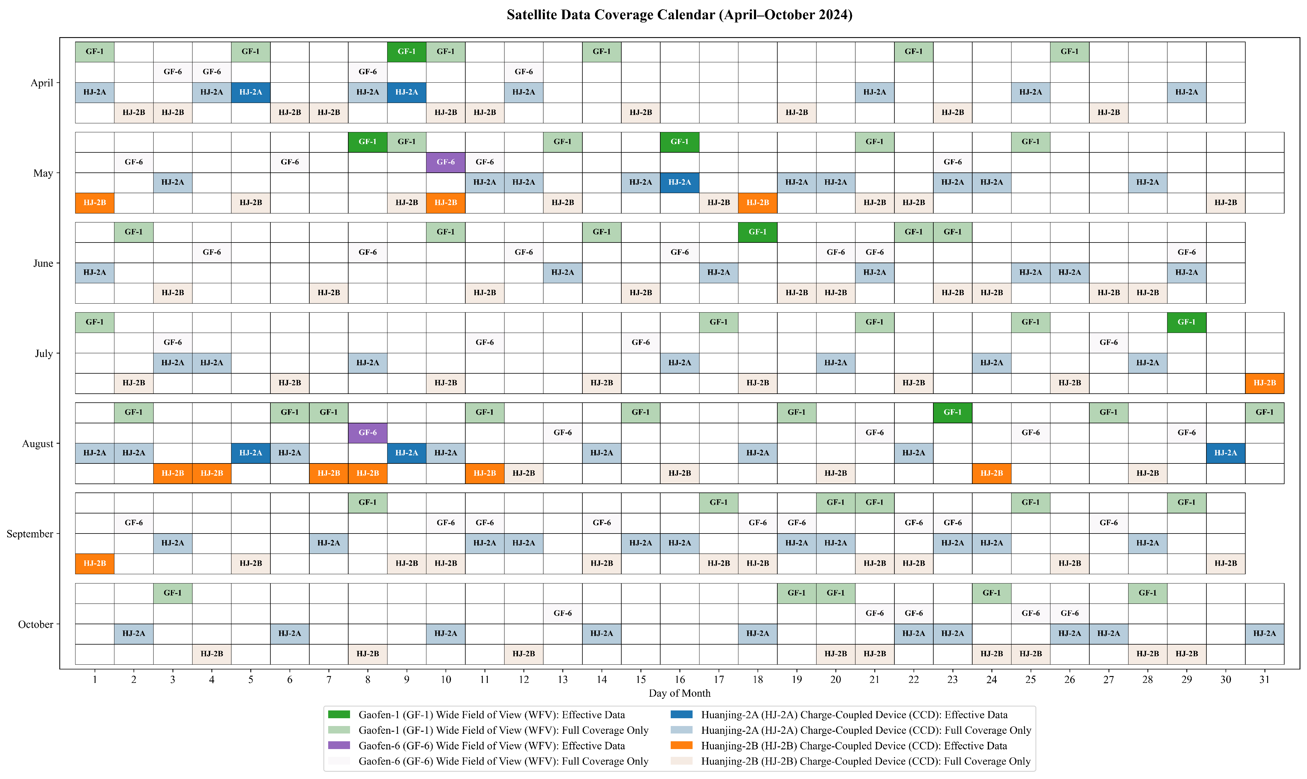In addition, some researchers have explored the integration of optical data and Synthetic Aperture Radar (SAR)—such as Sentinel-1 SAR—to improve the accuracy of aquatic vegetation classification [23,29,30]. Nevertheless, medium- to high-resolution multispectral satellites like Sentinel-2 MSI and the Landsat series typically have revisit periods of at least five days. During the peak growing season of aquatic vegetation in the Yangtze River Basin—when clear-sky conditions are scarce—it is often challenging to acquire valid imagery. Although SAR data such as Sentinel-1 can penetrate clouds, it cannot effectively penetrate the water surface, limiting its ability to capture information on submerged vegetation. To address the challenge that existing medium- to high-resolution optical satellites have relatively long revisit cycles—making it difficult to obtain sufficient cloud-free imagery during the peak growing season of aquatic vegetation—this study aims to develop a high-temporal-resolution dataset (effective revisit interval of about one day) by integrating imagery from China’s Gaofen-1/6 (GF-1/6) Wide Field of View (WFV) sensors and Huanjing-2A/B (HJ-2A/B) Charge-Coupled Device (CCD) instruments. Building on this dataset, we leverage the strong spectral–spatial feature learning capability of deep learning algorithms to investigate its potential for high-precision aquatic vegetation classification.

2. Materials

2.1. Study Area

This study selected six representative lakes within China’s Yangtze River Basin for the purpose of sampling (Figure 1), including Lake Taihu, Lake Chaohu, Lake Honghu, Lake Dianchi, Lake Dianshanhu, and Lake Caohai. These lakes are evenly distributed along the main course of the Yangtze River, spanning its upper (Lakes Dianchi and Caohai), middle (Lake Honghu), and lower reaches (Lakes Chaohu, Taihu and Dianshanhu), thus encompassing the basin’s major hydrological segments. The selected lakes exhibit both representativeness and diversity in the composition of aquatic vegetation life forms. As shown in

Table 1. Life-form composition of aquatic vegetation across different lakes.

Lake	Submerged Vegetation (SV)	Floating-Leaved (FV)	Emergent Vegetation (EV)
Lake Taihu	✓	✓	✓
Lake Chaohu	×	✓	✓
Lake Honghu	×	✓	✓
Lake Dianchi	×	✓	✓
Lake Dianshanhu	✓	✓	✓
Lake Caohai	×	✓	✓

, each lake supports at least two of the three dominant life forms—submerged, floating-leaved, and emergent plants—providing a comprehensive representation of aquatic vegetation growth conditions across the Yangtze River Basin [31]. The region lies within the subtropical monsoon climate zone, where rainfall and warmth occur concurrently [32]. The growing season of aquatic vegetation typically spans from April to October, with peak biomass observed during August and September [27,33,34,35]. During this period, the area is predominantly influenced by monsoonal circulation, resulting in frequent overcast and rainy weather [36,37].

Lake Taihu (30°55′N–31°34′N, 119°53′E–120°36′E), China’s third-largest freshwater lake, is located at the center of the Yangtze River Delta. The basin is one of the country’s most economically developed regions, with its population in 2024 accounting for 4.9% of China’s total and its GDP contributing 10.1% to the national economy [38], reflecting the intensity of human activities. The region experiences a subtropical monsoon climate with distinct seasons, abundant warmth, and plentiful rainfall. The long-term mean temperature ranges from 15 to 17 °C, and the average annual precipitation is approximately 1177 mm. Lake Taihu supports three primary life forms of aquatic vegetation—submerged, floating-leaved, and emergent species—showing a spatial pattern of sparse growth in the northern and western zones, while being widely distributed across the northeastern, eastern, and southern parts of the lake [39]. Given its large surface area, complex aquatic vegetation community, and the coexistence of intensive human activities with relatively complete lake ecosystems, Lake Taihu serves as a representative site for exploring the interactions between anthropogenic disturbances and aquatic vegetation dynamics in the Yangtze River Basin.

2.2. Image Data

The remote sensing data utilized in this study primarily consist of images from the GF-1/6 WFV and HJ-2A/B CCD satellites. GF-1, launched in April 2013, and GF-6, launched in June 2018, are both equipped with WFV sensors offering a spatial resolution of 16 m. Each satellite has an individual revisit period of 4 days, which shortens to 2 days when operating in tandem. Similarly, the HJ-2A and HJ-2B satellites, launched in September 2020, carry CCD sensors with multispectral bands of the same 16 m spatial resolution and a 4-day revisit cycle, reduced to 2 days in dual-satellite operation. When these four satellites function together as a complete observation network, the theoretical revisit frequency can be further improved to once per day. Taking Lake Taihu from April to October 2024 as an example (Figure 2). Over a total observation period of 214 days, complete satellite coverage was achieved on 173 days, of which 21 days provided high-quality imagery characterized by minimal cloud cover and sun glints.

The spectral bands for each sensor are listed in

Table 2. Spectral band configuration of Chinese domestic satellites.

	Sensor	GF-1 WFV	GF-6 WFV	HJ-2A CCD	HJ-2B CCD
Band
B1		450–520	450–520	450–520	450–520
B2		520–590	520–590	520–590	520–590
B3		630–690	630–690	630–690	630–690
B4		770–890	770–890	770–890	770–890
B5		/	690–730	690–730	690–730
B6		/	730–770	/	/
B7		/	400–450	/	/
B8		/	590–630	/	/

Note: “/” denotes the absence of the corresponding spectral band in that sensor.

. This study mainly utilized the common spectral bands shared by all sensors—the blue (B1), green (B2), red (B3), and near-infrared (B4) bands—for analytical purposes. All satellite imagery used in this research is available from the China Centre for Resources Satellite Data and Application (CRESDA) (https://data.cresda.cn/#/home, accessed on 1 April 2025).

2.3. Field Validation Data

The validation areas for aquatic vegetation distribution were delineated through a comprehensive analysis combining historical literature and remote sensing interpretation results, with survey timing adjusted according to weather conditions and satellite overpass schedules. A standardized quadrat sampling method was employed to validate the spatial distribution patterns of aquatic vegetation in the field. Considering both the spatial resolution of the satellite imagery and the operational feasibility of fieldwork, each quadrat was uniformly designed as a 10 × 10 m². By integrating ground-based observations with aerial imagery acquired via unmanned aerial vehicles (UAVs), the study conducted a systematic investigation and quantitative evaluation of aquatic vegetation community types and their coverage across the study area.

Between August 2023 and October 2024, eight systematic field validation surveys were conducted across all lakes within the study area. A total of 121 sampling points of aquatic vegetation distribution were obtained, comprising 38 sites of submerged vegetation, 9 of floating-leaved vegetation, 40 of emergent vegetation, and 34 of background categories. The spatial distribution of these validation sites is shown in Figure 3.

2.4. Measured Spectral Data

In this study, an Analytical Spectral Devices (ASD) FieldSpec spectroradiometer (Malvern Panalytical, Malvern, United Kingdom) was used to measure the spectral characteristics of aquatic vegetation and water bodies. Given that different life forms of aquatic vegetation vary in their vertical positioning relative to the water surface, resulting in distinct spectral features, a differentiated measurement strategy was applied. For submerged vegetation and open water, above-water spectral measurements were performed to effectively separate water-leaving radiance from atmospheric scattering signals [40], whereas for floating-leaved and emergent vegetation, conventional field spectral measurement methods were used to directly obtain canopy reflectance.

Field validation and supplementary water body experiments were conducted under clear and cloud-free conditions. A total of 78 reflectance spectra were obtained, representing four categories: submerged vegetation (n = 13), floating-leaved vegetation (n = 10), emergent vegetation (n = 25) and open water (n = 30) (Figure 4a–d). The spectral data of various surface features were averaged, together with algal bloom spectra, used to generate characteristic reflectance curves for different surface types (Figure 4e). Results indicate that in the visible wavelength range, water shows slightly higher reflectance than other surfaces, with submerged vegetation exhibiting the lowest reflectance. In the near-infrared range, emergent vegetation demonstrate the typical high-reflectance pattern of green vegetation, greatly exceeding that of floating-leaved vegetation, algal blooms, and submerged vegetation, while water remains the darkest target.

3. Methods

3.1. Image Preprocessing

Using Sentinel-2 MSI orthorectified imagery provided by European Space Agency (ESA) (https://browser.dataspace.copernicus.eu/, accessed on 1 April 2025, 10 m spatial resolution), together with SRTM DEM data (https://dwtkns.com/srtm30m/, accessed on 1 April 2025, 30 m spatial resolution), we refined the original RPC model of the domestic satellites and applied the corrected RPC model to geometrically rectify the imagery [41,42,43,44].

Radiometric calibration was applied to the geometrically corrected images using the official calibration coefficients released by CRESDA (https://mp.weixin.qq.com/s/uREY-V33lQTPqNlCtKuuww, accessed on 1 April 2025), converting raw DN values into spectral radiance. For historical images, absolute radiometric calibration coefficients published within six months before or after the imaging date were adopted. For recent images, if coefficients within that six-month window were unavailable, the latest officially released values were used. This approach ensured that the interval between image acquisition and coefficient generation never exceeded 15 months, thereby maintaining the reliability of radiometric calibration.

Finally, atmospheric correction was performed using radiative transfer models such as 6S [45,46,47,48] or MODTRAN [49,50], converting top-of-atmosphere radiance into surface reflectance. The models simulate atmospheric scattering and absorption processes while incorporating site-specific atmospheric parameters at the time of acquisition—such as aerosol type and water vapor content—to effectively eliminate atmospheric effects and improve spectral fidelity. Based on the study area’s geographic setting, imaging date, and data quality, the atmospheric model was configured as mid-latitude summer, the aerosol model as rural, and visibility was set to 23 km, ensuring high-accuracy atmospheric correction.

3.2. Equivalent Reflectance Computation

Using measured spectral data together with the spectral response function (SRF) provided by CRESDA (https://mp.weixin.qq.com/s/uREY-V33lQTPqNlCtKuuww, accessed on 1 April 2025), the equivalent surface reflectance of each band was derived through convolution integration [51]. Given the differences in spectral measurement approaches for various surface types, appropriate equivalent reflectance computation methods were adopted for each category.

For submerged vegetation and open-water surfaces, the equivalent water remote sensing reflectance ($R_{\mathrm{rs}}$) was derived from field measurements and subsequently multiplied by $\pi$ to obtain the equivalent surface reflectance (R) [52]. The corresponding computation was expressed as

$$\left\{\begin{array}{cc}\hfill R_{\mathrm{rs}}\left(ban{d}_i\right)& ={\displaystyle \frac{{\int }_{{\lambda }_1}^{{\lambda }_2}{R}_{\mathrm{rs}}\left(\lambda \right)SRF\left(\lambda \right)d\left(\lambda \right)}{{\int }_{{\lambda }_1}^{{\lambda }_2}SRF\left(\lambda \right)d\left(\lambda \right)}},\hfill \\ \hfill R\left(ban{d}_{\mathrm{i}}\right)& =R_{\mathrm{rs}}\left(ban{d}_{\mathrm{i}}\right)\times \pi .\hfill \end{array}\right.$$

(1)

where $R_{\mathrm{rs}}\left(ban{d}_{\mathrm{i}}\right)$ denotes the equivalent water remote-sensing reflectance for the i-th spectral band (${\mathrm{sr}}^{-1}$), $R_{\mathrm{rs}}\left(\lambda \right)$ is the measured water remote sensing reflectance (${\mathrm{sr}}^{-1}$), and ${\lambda }_1$ to ${\lambda }_2$ denote the wavelength range of the band.

The equivalent surface reflectance of floating-leaved and emergent vegetation was calculated using the following formula:

$$R\left(ban{d}_{\mathrm{i}}\right)={\displaystyle \frac{{\int }_{{\lambda }_1}^{{\lambda }_2}R\left(\lambda \right)SRF\left(\lambda \right)d\left(\lambda \right)}{{\int }_{{\lambda }_1}^{{\lambda }_2}SRF\left(\lambda \right)d\left(\lambda \right)}}$$

(2)

where $R\left(ban{d}_{\mathrm{i}}\right)$ represents the equivalent surface reflectance for the i-th spectral band, while $R\left(\lambda \right)$ refers to the measured surface reflectance, and ${\lambda }_1$ to ${\lambda }_2$ denote the wavelength range of the band.

3.3. Remote Sensing Interpretation Features

This study differentiated various surface types primarily by analyzing their spectral and textural characteristics, as summarized in

Table 3. Remote sensing interpretation characteristics of different surface types.

Class	True Color Composite	False Color Composite	Description
Submerged Vegetation (SV)			Appears dark green or nearly black in true color composites, and dark red or black in false color composites, exhibiting a rough surface-like distribution.
Floating-leaved Vegetation (FV)			Appears light green in true color composites, and pale pink in false color composites, distributed in rough surface-like or fragmented patterns along the lakeshore.
Emergent Vegetation (EV)			Appears bright to dark green tones in true color composites, and bright pink to red tones in false color composites, distributed in rough surface-like patterns along the lakeshore.
Water			Appears blue or black in both true, and false color composites, showing a smooth surface-like distribution.
Algal Bloom (AB)			Appears bright green in true color composites, and bright pink in false color composites, showing a smooth flocculent distribution.

.

3.4. Sample Preparation

The study defined the lake boundary as the spatial reference for sample generation. Remote sensing imagery containing only the near-infrared, red, and green bands was cropped to produce raster image datasets, and the corresponding classification vector data were converted into label rasters of identical spatial extent. Using a fixed-size sliding window with a 10% overlap and zero-padding along the boundaries, spatially aligned image–label pairs of 256 × 256 pixels were generated. To address the class imbalance caused by the dominance of background pixels such as open water and algal bloom, all pairs consisting solely of background classes were excluded, resulting in 836 valid sample pairs. Given the intensive workload involved in manual interpretation of aquatic vegetation types, data augmentation techniques were employed to enhance dataset diversity and utilization. Augmentation methods included rotations of 90° and 270°, horizontal and vertical flips, and diagonal mirroring. After augmentation, the dataset expanded to 5016 pairs, which were subsequently divided into training and validation sets at a ratio of 8:2.

3.5. Network Model Architecture

This study employed an advanced encoder–decoder segmentation framework, namely U-Net++ integrated with an EfficientNet-B5 backbone. The encoder was initialized with weights pretrained on the ImageNet dataset, leveraging transfer learning to enhance the efficiency and robustness of multi-scale feature extraction—from high-level semantic representations to fine-grained textural details—across multi-channel remote sensing imagery. The decoder adopted the U-Net++ architecture, an enhanced version of the classic U-Net, characterized by its densely nested skip connections that allow more precise fusion of hierarchical features captured at different encoding stages [53]. By combining EfficientNet’s powerful feature representation with U-Net++’s superior capability in reconstructing spatial details and object boundaries, this hybrid architecture provided a robust foundation for the precise segmentation of aquatic vegetation with complex morphological structures.

3.6. Experimental Settings

All experiments were implemented on an NVIDIA GeForce RTX 4080 SUPER GPU equipped with 16 GB of memory. To balance model performance, contextual feature capture, and computational efficiency, the input image size was normalized to 256 × 256 pixels, with a batch size of 4. The segmentation framework combined U-Net++ and an EfficientNet-B5 backbone, optimized for a four-class classification task. Parameter updates were carried out using the Adam optimizer, with an initial learning rate of $1\times {10}^{-4}$ that decayed progressively to $1\times {10}^{-6}$ following a cosine annealing schedule.

A hybrid loss function integrating Dice Loss and Focal Loss was designed to improve recognition of underrepresented classes. To mitigate overfitting, training was run for 200 epochs with an early stopping criterion—halting automatically if validation performance showed no improvement for 20 consecutive epochs. Validation was executed after each epoch, and model checkpoints were saved every five epochs to ensure training stability and traceability.

3.7. Model Evaluation

3.7.1. Source of Evaluation Data

To thoroughly evaluate the model’s classification performance, this study utilized multi-source validation datasets. The visual interpretation results derived from remote sensing imagery provided polygonal reference data representing the distribution of aquatic vegetation, while field validation provided point-based ground truth samples. Together, these datasets formed a comprehensive, multi-scale validation framework. This integrative approach allowed simultaneous evaluation of the model’s capability to capture large-scale spatial patterns and its performance in localized classifications, ensuring a systematic and robust assessment of overall model performance.

3.7.2. Evaluation Method Design

Surface reference data were generated from Sentinel-2 MSI imagery acquired on the same date as the target image with a higher spatial resolution of 10 m. Using the spectral, textural, and spatial distribution features of aquatic vegetation, manual visual interpretation was performed to delineate high-accuracy reference polygons. Within the study region, we selected three representative lakes for model evaluation: Lake Taihu, the largest lake with extensive and highly diverse aquatic vegetation; Lake Chaohu, the second largest but characterized by sparse vegetation and relatively few life forms; and Lake Caohai, the smallest lake, where vegetation is widely distributed but exhibits low diversity.

A point-based validation dataset was established by integrating field validation data collected under favorable weather conditions with temporally and spatially matched remote sensing imagery. Given the temporal stability of aquatic vegetation spectral characteristics [33,35] and the scarcity of clear-sky days that constrained the acquisition of high-quality imagery, we selected high-quality images acquired within 15 days of the field validation and excluded from model training as the matching data source. Due to field access limitations, boat-based observations were restricted to the marginal zones of aquatic vegetation, making it challenging to capture pure vegetation pixels. Thus, a coverage threshold of 50% was defined as the minimum level of aquatic vegetation that can be reliably detected through remote sensing. Furthermore, to account for GPS positioning errors, vessel drift caused by wind and water currents, and to minimize uncertainties in spatial distribution and coverage due to temporal differences between imagery and field data, a buffer zone with a 50 m radius (approximately three pixels) centered on each sampling point was established. Classification results were deemed correct when at least one classified pixel within the buffer zone matched the corresponding field observation.

3.7.3. Evaluation Metrics

A pixel-level, dual-dimensional assessment framework was employed in this study. Class-level evaluation metrics were used to quantify the model’s capability in distinguishing individual categories, while overall metrics was applied to evaluate its global classification performance. This integrated approach enabled a comprehensive evaluation of the model from both local and overall perspectives.

(1)

Class Evaluation

The classification performance for each category was assessed using standard evaluation metrics, including Intersection over Union (IoU), Precision, Recall, and F1-Score. The corresponding formulas are presented as

$$IoU={\displaystyle \frac{TP}{TP+FP+FN}}$$

(3)

$$Precision={\displaystyle \frac{TP}{TP+FP}}$$

(4)

$$Recall={\displaystyle \frac{TP}{TP+FN}}$$

(5)

$$F1-Score={\displaystyle \frac{2\times Precision\times Recall}{Precision+Recall}}={\displaystyle \frac{2\times TP}{2\times TP+FP+FN}}$$

(6)

where $TP$ represents the number of correctly classified positive pixels, $FP$ represents the number of negative pixels misclassified as positive, and $FN$ represents the number of positive pixels misclassified as negative.

(2)

Overall Evaluation

The overall classification performance was evaluated using four standard metrics: mean Intersection over Union (mIoU), mean Pixel Accuracy (mPA), Overall Accuracy (OA), and the Kappa coefficient.

The mIoU metric quantifies the overlap between predicted and reference regions, and is calculated as

$$mIoU={\displaystyle \frac{1}{n}}\times \sum _{\mathrm{i}=1}^{\mathrm{n}}Io{U}_{\mathrm{i}}$$

(7)

where $Io{U}_{\mathrm{i}}$ denotes the Intersection over Union for the i-th category, and n represents the total number of categories.

Overall Accuracy (OA) evaluates the model’s global classification correctness across all pixels, serving as an indicator of its overall performance. Mean Pixel Accuracy (mPA), on the other hand, assesses the model’s per-class pixel-level accuracy, providing insight into its ability to distinguish minor or less represented classes. The corresponding formulas are expressed as

$$OA={\displaystyle \frac{{\sum }_{\mathrm{i}=1}^{\mathrm{n}}T{P}_{\mathrm{i}}}{N}}$$

(8)

$$mPA={\displaystyle \frac{1}{n}}\times \sum _{\mathrm{i}=1}^{\mathrm{n}}{\displaystyle \frac{T{P}_{\mathrm{i}}}{T{P}_{\mathrm{i}}+F{N}_{\mathrm{i}}}}$$

(9)

where $T{P}_{\mathrm{i}}$ represents the number of correctly classified pixels for the i-th class, and $F{N}_{\mathrm{i}}$ denotes the number of pixels from the i-th class that are incorrectly assigned to other categories, and N refers to the total number of pixels.

The Kappa coefficient quantifies the agreement between the model’s classification results and the ground truth, accounting for the possibility of random agreement. Its calculation is expressed as

$$Kappa={\displaystyle \frac{p_0-p_{\mathrm{e}}}{1-p_{\mathrm{e}}}}$$

(10)

where $p_0$ denotes the ratio of correctly classified pixels to the total number of pixels, corresponding to the Overall Accuracy (OA), and $p_{\mathrm{e}}$ is defined as follows:

$$p_{\mathrm{e}}={\displaystyle \frac{{\sum }_{\mathrm{i}=1}^n(T{P}_{\mathrm{i}}+F{N}_{\mathrm{i}})\times (T{P}_{\mathrm{i}}+F{P}_{\mathrm{i}})}{N\times N}}$$

(11)

where $F{P}_{\mathrm{i}}$ denotes the number of pixels from other categories that are incorrectly assigned to the i-th class.

3.8. Statistical Approaches and Error Analysis Techniques

Pearson’s correlation coefficient was used to quantify the relationship between the two datasets: image reflectance versus equivalent reflectance in the atmospheric correction assessment, and inter-sensor band-level reflectance consistency in the sensor consistency evaluation.

Root Mean Square Error (RMSE) was further applied to measure their quantitative differences, reflecting deviations from equivalent reflectance in the atmospheric correction analysis and discrepancies in band reflectance between the two sensors in the consistency assessment.

$$RMSE=\sqrt{{\displaystyle \frac{{\sum }_{\mathrm{i}=1}^{\mathrm{n}}{(X_{\mathrm{obs},\mathrm{i}}-X_{\mathrm{pred},\mathrm{i}})}^2}{n}}}$$

(12)

where $X_{\mathrm{obs},\mathrm{i}}$ represents observed data, and $X_{\mathrm{pred},\mathrm{i}}$ denotes predicted data, n stands for total number of observations.

4. Results

4.1. Atmospheric Correction Evaluation

Given the strong spatiotemporal variability of water optical properties and the comparatively stable spectral characteristics of aquatic vegetation, this study employed a data collection strategy integrating both synchronous and quasi-synchronous observations to assess atmospheric correction performance. For water bodies, strictly synchronous matching was performed between in situ spectra and satellite image data acquired on the same day. For aquatic vegetation, quasi-synchronous matching was conducted using spectra and imagery collected within 7 days, ensuring consistent surface cover types for the matched pixels. During data processing, the equivalent surface reflectance was derived from field spectra using SRF and quantitatively compared with the surface reflectance retrieved from corresponding image pixels. As illustrated in Figure 5, the validation results showed that most scatter points followed a well-aligned 1:1 linear relationship, with Pearson’s r consistently exceeding 0.83 (p < 0.001) and RMSE remaining below 0.115. These findings confirm that the atmospheric correction approach employed in this study provides high accuracy and robustness.

4.2. Sensor Consistency Evaluation

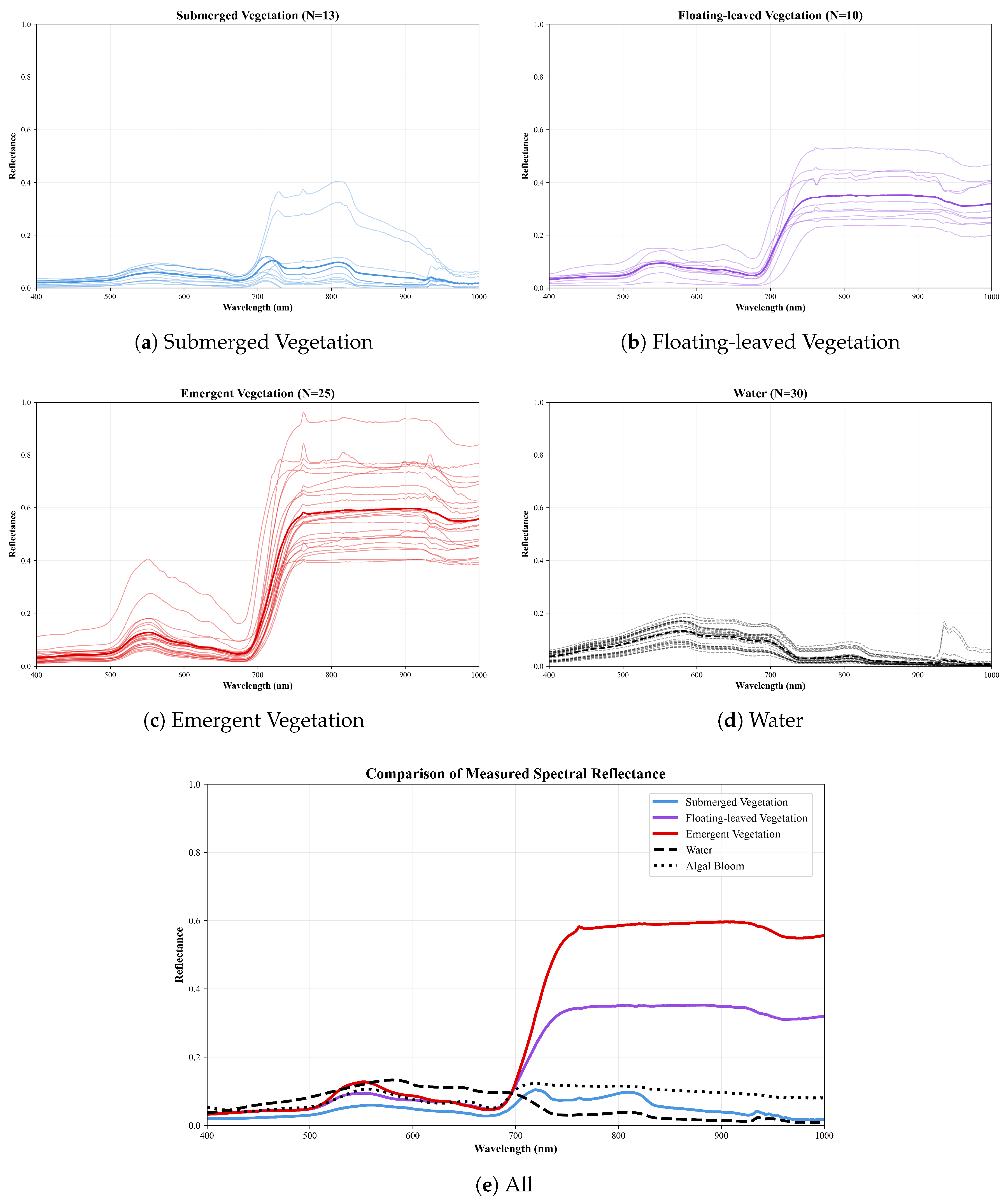
In this study, Chinese domestic multispectral satellite data were jointly employed for model development, incorporating imagery from multiple sensors, including GF-1 WFV (four cameras), GF-6 WFV (one camera), and HJ-2A/B CCD (four cameras). As shown in Figure 6, inherent differences among the Spectral Response Functions (SRFs) of these sensors can introduce systematic deviations in surface reflectance products. To ensure the effective integration of multisensor datasets within the deep learning framework, we conducted a twofold evaluation of spectral consistency: (1) simulating and comparing sensor-specific reflectance using in situ surface spectra combined with each sensor’s SRF; and (2) directly comparing surface reflectance products derived from quasi-synchronous imagery. This comprehensive assessment enabled a quantitative analysis of the spectral discrepancies among reflectance products generated by different sensors.

4.2.1. Sensor Consistency Evaluation Based on Spectral Response Function

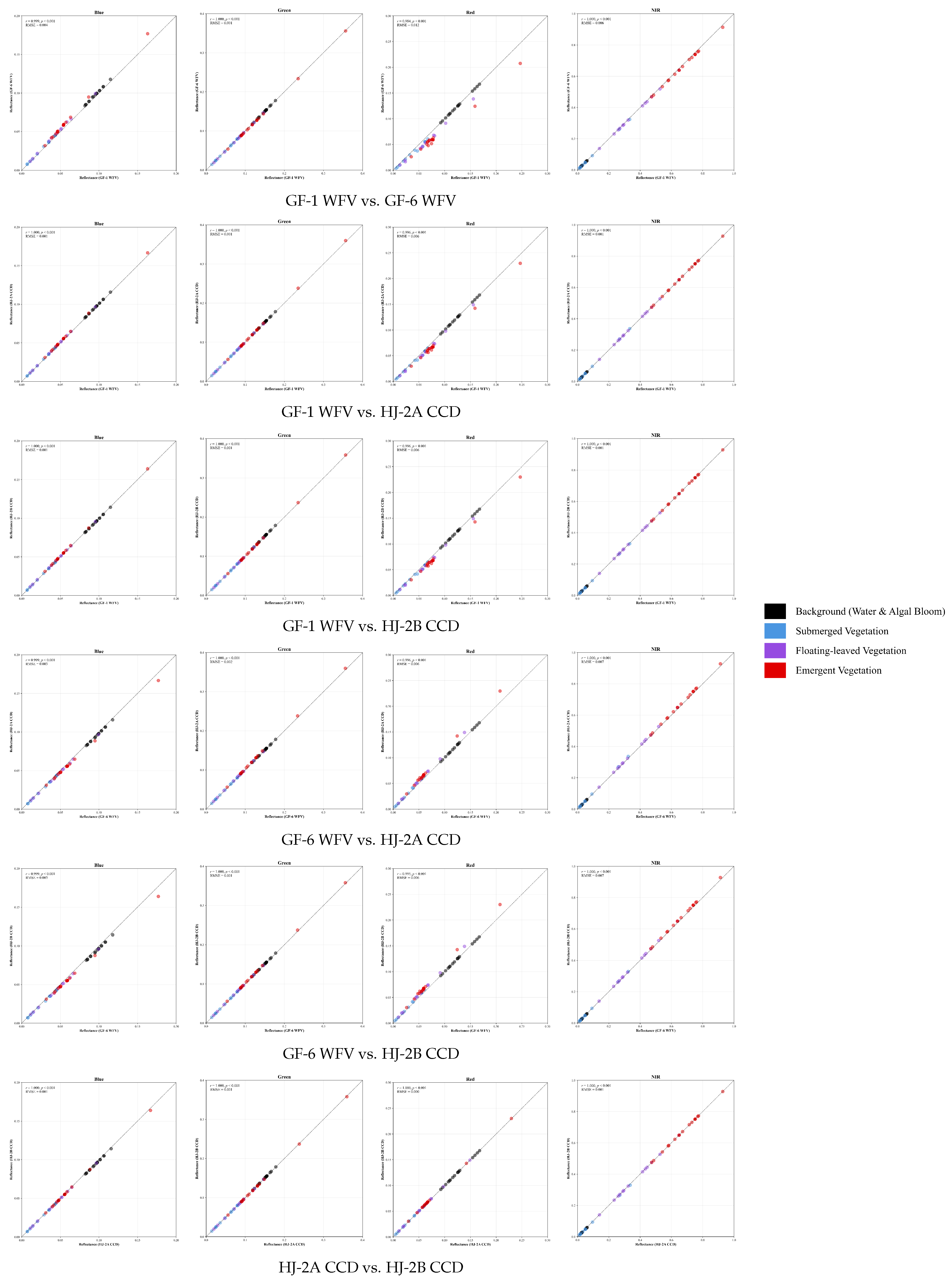
For multi-camera mosaic sensors, the equivalent surface reflectance of each camera was first derived using the in situ spectra and the respective SRF of each camera. The equivalent reflectances from all cameras within a single sensor were then averaged to represent the overall equivalent surface reflectance of that sensor. Cross-validation of band-matched equivalent reflectance across different sensors (Figure 7) demonstrates that scatter points for all bands align closely with the 1:1 reference line. Pearson’s r exceeds 0.81 for every band (p < 0.001), and RMSE remains below 0.012, indicating strong spectral consistency among sensors.

4.2.2. Sensor Consistency Evaluation Based on Quasi-Synchronous Imagery

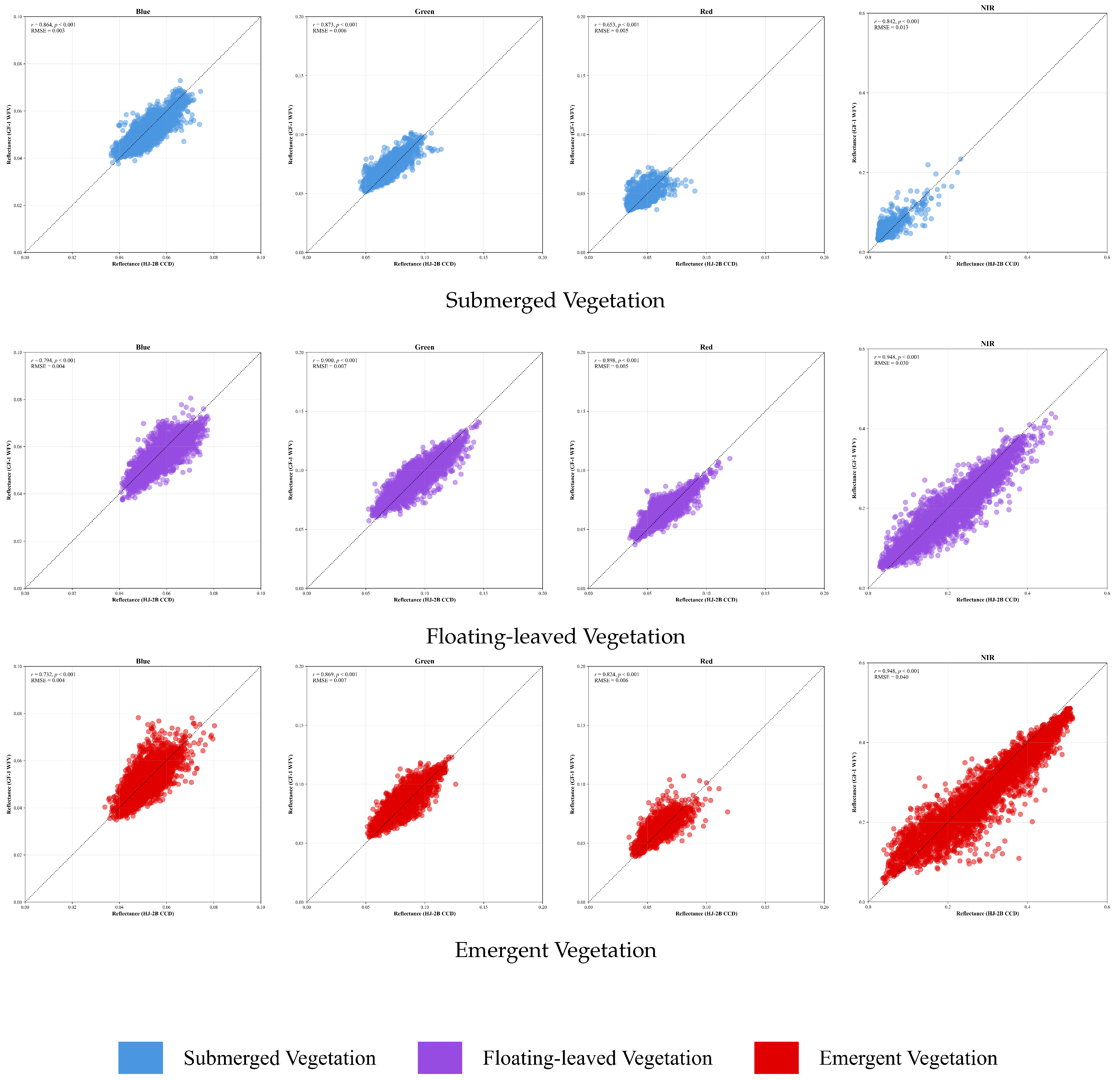
Due to the scarcity of clear-sky conditions in the study area, it is difficult to obtain perfectly synchronous multi-source satellite data. To address this, we selected a pair of quasi-synchronous images—a GF-1 WFV scene acquired on 23 August, 2024, and an HJ-2B CCD scene captured one day later—to evaluate sensor consistency at the surface reflectance level. To precisely assess the spectral consistency of specific surface categories, the imagery was overlaid with a pre-established vector dataset representing aquatic vegetation classifications for comparative analysis. Due to the highly variable optical characteristics of water bodies, their spectral signatures can change noticeably even within a single day, while the spatial distribution of algal blooms also shifts over time. Consequently, this study excluded background pixels such as open water and algal bloom areas, concentrating instead on comparing the reflectance of the three primary aquatic vegetation types—submerged, floating-leaved, and emergent vegetation. As shown in Figure 8, the reflectance scatter points of all three aquatic vegetation life forms cluster closely around the 1:1 reference line across all spectral bands. Pearson’s r exceeds 0.65 for each band (p < 0.001), and the RMSE remains below 0.040, demonstrating strong spectral consistency between the two sensor datasets.

Combining the results from SRF simulations and quasi-synchronous imagery cross-validation, this study demonstrates that the four selected sensors maintain strong spectral consistency in surface reflectance products. Therefore, additional cross-sensor normalization or calibration is unnecessary. This finding suggests that these heterogeneous datasets are suitable for collaborative classification and can provide a solid data basis for building a unified joint model.

4.3. Selection of Input Parameters and Model Components

In remote sensing image semantic segmentation, the selection of input parameters can strongly influence model performance. To verify the rationality and necessity of the input configurations used in this study, comparative experiments were conducted from two aspects: input band combinations and input block size. All experiments were performed under the same training strategy and network architecture, with each configuration tested in three repeated trials.

First, in terms of input bands, we tested three configurations: using only near-infrared, red, and green (NIR + R + G); adding the blue band; and adding the normalized difference vegetation index (NDVI). As shown in

Table 4. Selection of input parameters.

Exp.	Input Band	Input Block Size	mIoU ± std (%)	mPA ± std (%)
Final Model	NIR + R + G	$256\times 256$	$77.49\pm 1.15$	$84.65\pm 1.30$
+ Blue	NIR + R + G + B	$256\times 256$	$76.06\pm 0.22$	$83.48\pm 0.42$
+ NDVI	NIR + R + G + NDVI	$256\times 256$	$72.73\pm 0.96$	$81.30\pm 0.51$
+ Input Size	NIR + R + G	$\mathbf{128}\times \mathbf{128}$	$73.69\pm 1.49$	$81.42\pm 1.26$

Note: bold text indicates input-parameter settings that differ from those used in the final model configuration.

, the NIR + R + G configuration achieved the most favorable performance across three trials, outperforming the other setups. This indicates that including additional bands such as blue or NDVI can introduce redundancy, potentially increasing the model’s learning complexity and reducing its generalization capability.

Secondly, in terms of input block size, some lakes are relatively small, with dimensions less than 512 pixels, making the use of $512\times 512$ image blocks for training and prediction prone to errors. Therefore, we focused on testing $256\times 256$ and $128\times 128$ block sizes. The results indicated that the $256\times 256$ size provides an optimal balance between performance and computational efficiency, while smaller blocks ($128\times 128$) suffer from lower performance due to limited spatial context.

In conclusion, the experiments demonstrate that using the NIR + R + G band combination along with a $256\times 256$ input block size represents the optimal configuration for this task. This setup achieves a balance between computational efficiency and enhanced model performance and robustness, offering a solid experimental basis for further model comparisons and practical applications.

Based on the identified optimal input configuration (band combination and input block size), a series of comparative experiments were designed to systematically evaluate the effectiveness of each component in the final segmentation model and its contribution to overall performance.

Specifically, key modules of the model architecture, including the encoder, decoder, and loss function, were individually tested by removing or substituting them to quantify performance changes. As illustrated in

Table 5. Selection of model components.

Exp.	Encoder	Decoder	Loss	mIoU ± std (%)	mPA ± std (%)
Final Model	EfficientNet-B5	U-Net++	Dice + Focal	77.49 ± 1.15	84.65 ± 1.30
Loss	EfficientNet-B5	U-Net++	Cross Entropy	76.51 ± 1.08	83.67 ± 0.92
Encoder	ResNet-34	U-Net++	Dice + Focal	76.90 ± 1.16	84.36 ± 1.06
Decoder	EfficientNet-B5	U-Net	Dice + Focal	76.41 ± 0.07	83.24 ± 0.16

Note: bold text highlights model-component modifications relative to the final model architecture.

, these experiments provided insights into how each component contributes to performance improvement and confirmed the rationality and necessity of the modeling approach proposed in this study.

4.4. Model Performance

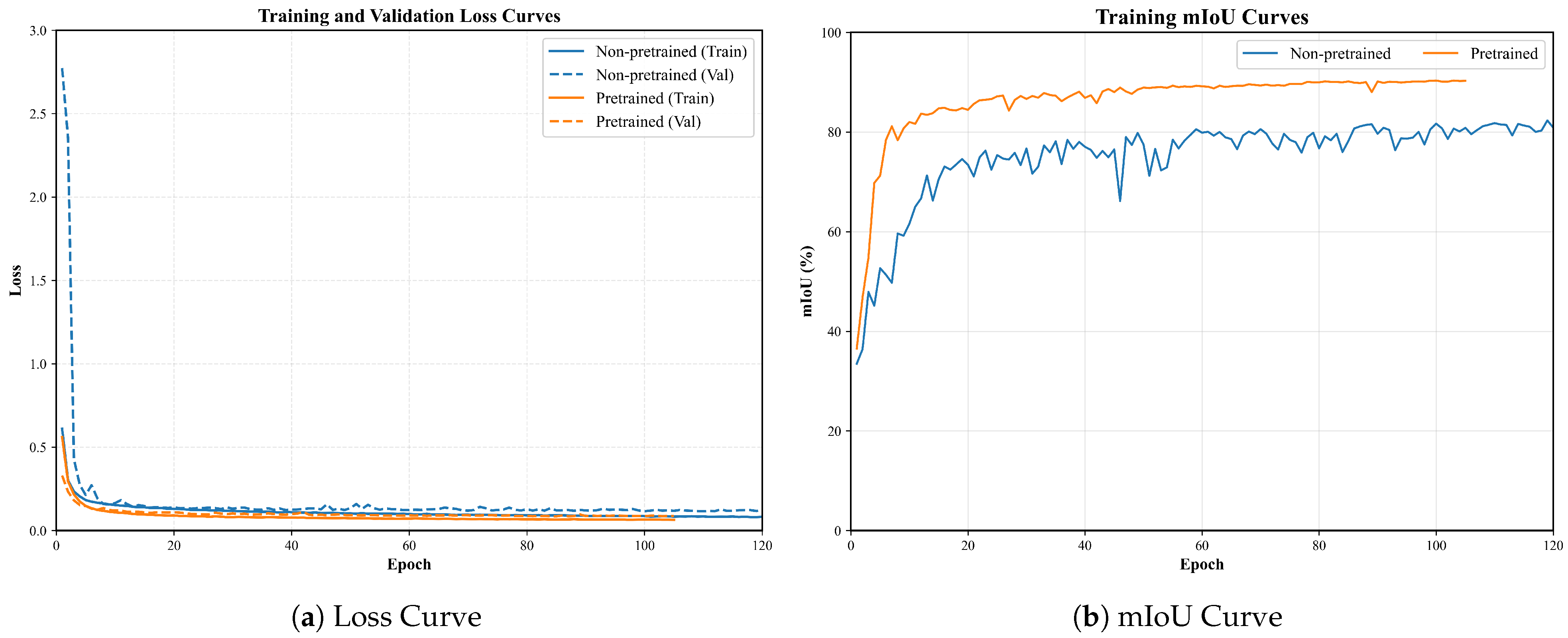
The model performance stabilized after around ten training epochs, where the training loss converged to 0.066, the validation loss to 0.086, and the training mIoU surpassed 90%. As shown in Figure 9, without transfer learning, both the validation loss and training mIoU fluctuated noticeably and failed to converge effectively. Ultimately, the optimal model demonstrated robust performance on the validation set, with an mIoU of 90.16%, an mPA of 95.27%, an OA of 99.11%, and a Kappa coefficient of 0.94.

To comprehensively assess the model’s classification performance, we established a multi-source validation framework. At the macro level, polygonal ground-truth data derived from visual interpretation were used to evaluate the spatial consistency of classification results. At the micro level, point-based field validation data were employed to examine the model’s local classification accuracy. This framework enables a multidimensional and systematic evaluation of the model’s classification capabilities.

4.4.1. Model Evaluation Based on Visual Interpretation

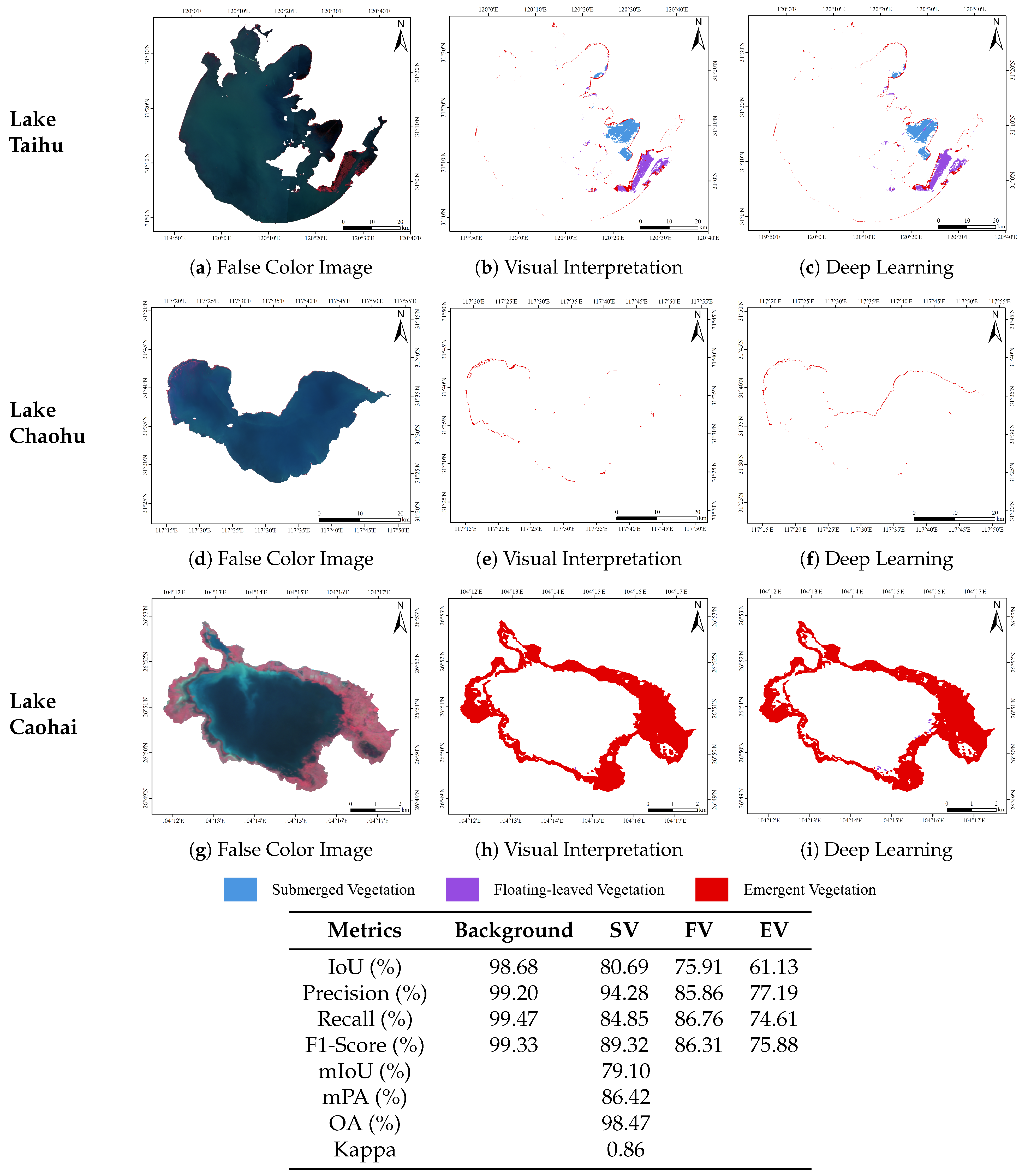
In this study, visually interpreted results from high-resolution Sentinel-2 MSI imagery (10 m spatial resolution) were used as benchmark ground truth to evaluate the model’s classification performance across a broad regional scale. Evaluation was conducted using a fully independent test dataset (Lake Taihu imagery acquired on 16 August 2020; Lake Chaohu on 12 August 2023; and Lake Caohai on 18 October 2024), which was strictly excluded from model training. As shown in Figure 10, the model achieved a relatively good overall performance, with mIoU = 79.10%, mPA = 86.42%, OA = 98.47%, and a Kappa coefficient of 0.86. At the class level, the IoU, Precision, Recall, and F1-Score for all aquatic vegetation life forms reached 61.13%, 77.19%, 74.61%, and 75.88%, respectively. Some confusion occurred between floating-leaved and emergent vegetation due to their similar spectral and textural characteristics, resulting in slightly lower classification performance for these types. Overall, the quantitative assessment confirms that the proposed deep learning model effectively captures the spatial distribution patterns of different aquatic vegetation life forms, highlighting its strong potential for large-scale aquatic vegetation monitoring via remote sensing.

4.4.2. Model Evaluation Based on Field Validation

Field validation data were used to evaluate the model’s classification performance in representative areas. Using field validation data collected under favorable weather conditions and remote sensing images obtained within a 15-day interval, a benchmark dataset comprising 101 field samples was established. These included 31 samples of submerged vegetation, 7 of floating-leaved vegetation, 29 of emergent vegetation, and 34 of background classes. As shown in Figure 11, the model achieved producer’s accuracies (PA) of 51.61% for submerged vegetation, 85.71% for floating-leaved vegetation, and 68.97% for emergent vegetation, while the user’s accuracies (UA) were 100%, 75.00%, and 90.91%, respectively. The OA reached 75.25%, with a Kappa coefficient of 0.65, indicating that the model maintains reliable classification performance in field-validated regions.

4.5. Comparison with Other Methods

We further compared our model with other widely adopted deep learning semantic segmentation frameworks. DeepLabv3+ excels at capturing multi-scale contextual information, making it particularly effective for large-scale and complex landscapes with diverse object sizes, while HRNet demonstrates superior performance in delineating fine boundaries and small-scale features due to its high-resolution feature maintenance mechanism. We performed three independent experimental runs for each algorithm. As illustrated in Figure 12, the model we trained achieves marginally higher mIoU and OA values compared with the other two models.

4.6. Spatiotemporal Variation of Aquatic Vegetation in Lake Taihu

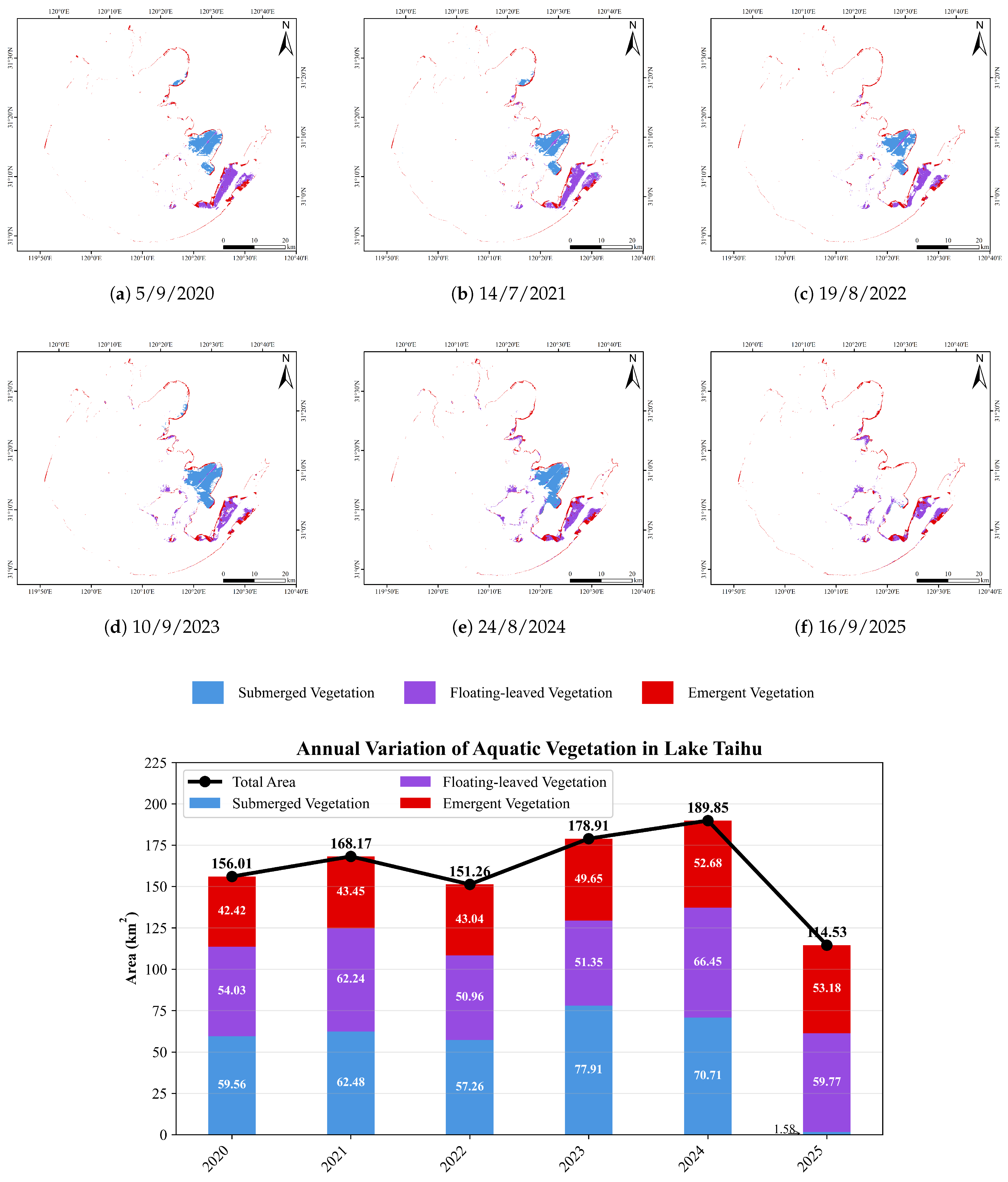
The trained deep learning model was employed to classify and extract remote sensing imagery of Lake Taihu captured during the peak growing season of aquatic vegetation over the past five years. Based on these classification results, the overall growth conditions of aquatic vegetation in Lake Taihu were analyzed. As illustrated in Figure 13, aquatic vegetation in Lake Taihu is primarily concentrated in the eastern portion of the lake. Submerged vegetation dominates the central region, while floating-leaved and emergent vegetation are mainly found in the southern area. These spatial patterns align well with previously reported field investigations and remote sensing observations [27,34,39]. The total area of aquatic vegetation in Lake Taihu peaked in 2024 at approximately $189.85{\mathrm{km}}^2$, then declined to its lowest level in 2025, about $114.53{\mathrm{km}}^2$.

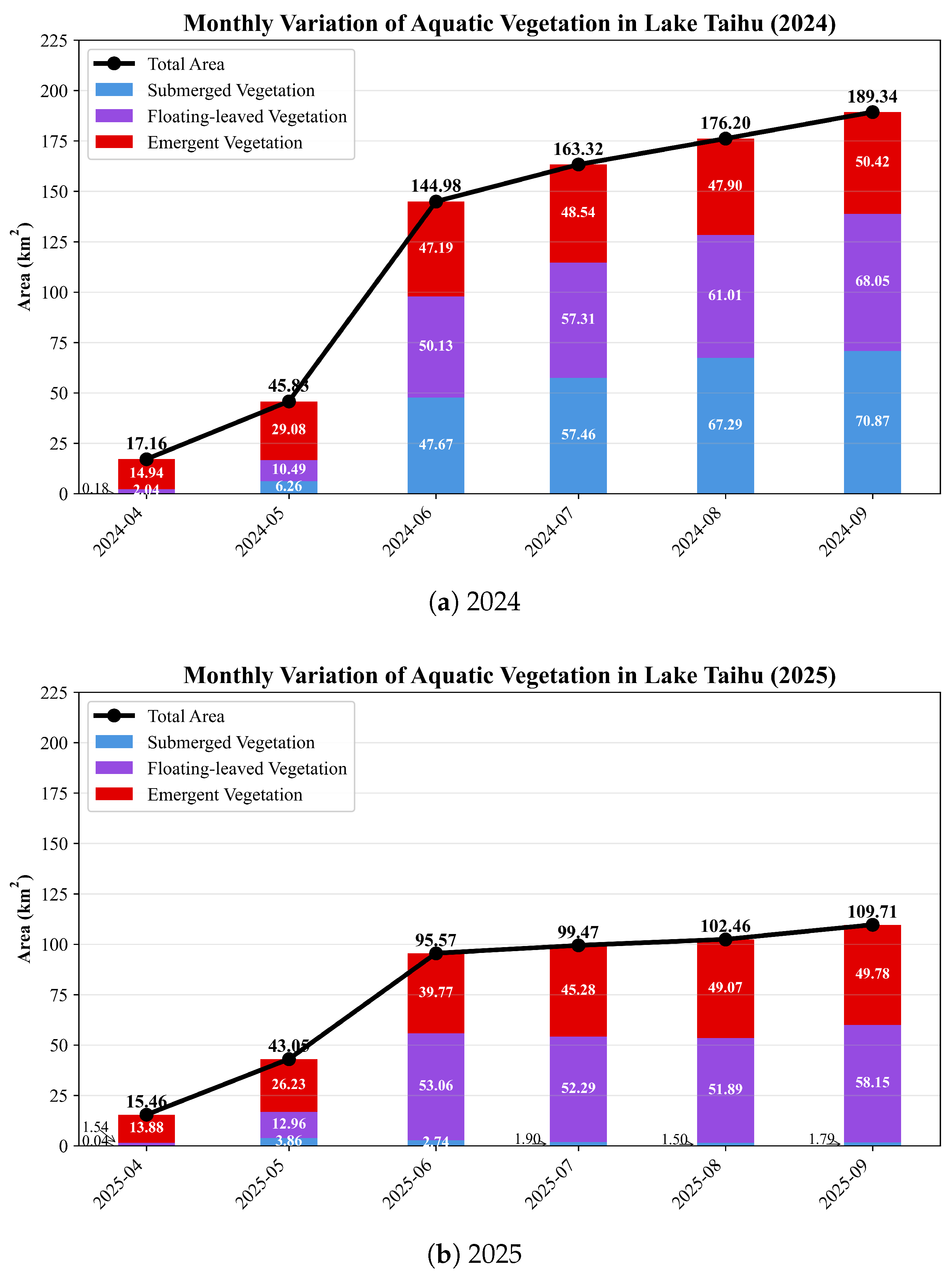
Based on multi-temporal satellite imagery from the growing seasons of 2024 and 2025—the years with the largest and smallest aquatic vegetation coverage in the past five years—aquatic vegetation was extracted and analyzed. The mean monthly aquatic vegetation area was used to characterize vegetation growth conditions in each month. As illustrated in Figure 14, aquatic vegetation is in its germination stage in April, enters a rapid growth phase from May to June, stabilizes gradually from July onward, and peaks around September.

Relative to other years, the total aquatic vegetation coverage in Lake Taihu in 2025 declined markedly, primarily due to the drastic degradation of submerged vegetation. A comparison of the monthly variations between 2024 and 2025 showed that the submerged vegetation area in 2025 had already fallen well below the previous year’s level by June and remained extremely low thereafter. To mitigate this decline, management agencies could strengthen water quality and water level regulation, enhance ecological monitoring, and conduct timely artificial replanting to restore submerged vegetation, thereby reducing algal blooms and curbing further eutrophication.

5. Discussion

In this study, we integrate domestic multispectral satellite observations (GF-1/6 WFV and HJ-2A/B CCD) with a deep learning classification framework to enable detailed mapping of lake aquatic vegetation across the Yangtze River Basin. Although deep learning has proven highly effective for automatically learning spatial–spectral representations and reducing reliance on handcrafted features, its use in this region has long been constrained by limited data sources and low observation frequency. For instance, despite the high spectral resolution and mature product system of Sentinel-2 MSI, persistent cloudy and rainy conditions during the peak growing season of aquatic vegetation (July–September) greatly restrict the availability of clear-sky imagery. To address this challenge, we incorporate multi-source domestic satellite imagery, reducing the effective revisit interval to approximately 1 day and substantially increasing the number of usable scenes and the timeliness of monitoring. Furthermore, by integrating U-Net++ with EfficientNet-B5, we develop a high-accuracy classification model whose mIoU and Kappa scores improve by 11% and 0.07, respectively, compared with previous work [28]. This framework provides a stronger data foundation and technical pathway for large-scale, high-frequency, and long-term remote sensing monitoring of aquatic vegetation.

Although our sample set includes several representative lakes—such as Lake Taihu, Lake Chaohu, and Lake Honghu—spanning diverse vegetation types and markedly different geographic settings, its spatial coverage is still limited. When the model is transferred to other lakes, variations in spectral signatures and spatial structural characteristics may reduce its accuracy in fine-grained classes, even if overall classification performance remains high. Moreover, the images used for sample construction were primarily acquired under favorable conditions with low cloud cover and minimal sun-glint contamination, while clouds and glint are common in real-world operational scenarios. Clouds obscure surface information outright, and sun glint makes it difficult for the model to recover the true characteristics of targets such as submerged vegetation. This often leads to missing or unretrievable vegetation patches—an inherent limitation of optical remote sensing in complex environments. Additionally, submerged vegetation is highly sensitive to water transparency, depth, chlorophyll-a concentration, and suspended matter levels [11,12], frequently resulting in situations where vegetation is clearly visible in the field but indistinguishable in satellite imagery. Consequently, even if evaluations based on visual interpretation appear promising, model performance may still be weaker when validated against in situ measurements.

To overcome these limitations, future research could improve usability and generalization along two directions. First, by taking advantage of the seasonal growth dynamics and relatively stable spatial patterns of aquatic vegetation, approaches incorporating spatial geometric constraints, neighborhood-based spatial inference, or temporal interpolation models could be employed to estimate vegetation conditions in areas obscured by dense clouds or strong sun glint. Such methods would help reduce spatiotemporal data gaps and enhance the completeness of monitoring results. Second, although domestic satellite constellations substantially increase the availability of optical imagery, some years or lake regions may still experience several consecutive weeks without usable scenes due to prolonged cloudy and rainy weather. To improve the continuity and robustness of long-term time-series monitoring, integrating Sentinel-1 or other SAR datasets as complementary sources would enable all-weather aquatic-vegetation observation through optical–radar data fusion, providing more reliable temporal information under challenging meteorological conditions.

In conclusion, the aquatic-vegetation monitoring framework developed in this study—combining Chinese domestic satellite imagery with deep learning—offers notable enhancements in image accessibility, model robustness, and the spatiotemporal continuity of monitoring. Moreover, it establishes a strong data and technical foundation for future studies on vegetation growth dynamics, exploration of ecological drivers, and the conservation of lake ecosystems in the Yangtze River Basin.

6. Conclusions

Based on 16 m spatial resolution domestic satellite data (GF-1/6 WFV and HJ-2A/B CCD), this study constructed aquatic vegetation sample sets for representative lakes in the Yangtze River Basin using visual interpretation. The datasets were split into training and validation sets at an 8:2 ratio. The U-Net++/EfficientNet-B5 model trained on the training set achieved high performance on the validation set, with mIoU = 90.16% and mPA = 95.27%. On independent test data derived from higher-resolution imagery (Sentinel-2 MSI) through visual interpretation, the model attained mIoU = 79.10% and mPA = 86.42%, with IoU and F1-Score for all aquatic vegetation life forms reaching 61.13% and 75.88%, respectively. Field-based evaluation yielded OA = 75.25% and Kappa = 0.65. When applied to peak-season images of Lake Taihu over the past five years, we found that aquatic vegetation in Lake Taihu is predominantly distributed in the eastern part of the lake, with total coverage peaking in 2024 and declining to its lowest in 2025, largely due to the drastic degradation of submerged vegetation.

The approach presented in this study offers reliable support for monitoring aquatic vegetation in lakes across the Yangtze River Basin. Our analysis demonstrates that the four sensors (GF-1/6 WFV and HJ-2A/B CCD) exhibit high consistency, satisfying the requirements for collaborative classification. Compared with other commonly used medium- to high-resolution satellites, these sensors provide substantially improved temporal coverage, providing more effective data during the peak growth period of aquatic vegetation when sunny days are limited. Furthermore, we identified that the sharp decline in Lake Taihu’s aquatic vegetation area in 2025 was primarily driven by the degradation of submerged vegetation, a trend that could be detected as early as June. This suggests that the technology developed in this study enables real-time monitoring of aquatic vegetation dynamics, facilitating early problem detection and timely management interventions.

It is important to note that, given the limited extent of the sample set, the model may show some inaccuracies when extended to other lakes, different river basins, or imagery impacted by clouds and complex weather conditions. Additionally, factors such as sun glint and water environment conditions can cause submerged vegetation to be visible in situ yet undetectable in remote sensing images, which can hinder the model’s ability to accurately extract these features.