Highlights
- Establish the submatrix dimension adaptive estimation model driven by coherence stability detection.
- Introduce the submatrix overlap criterion for covariance matrix adaptive sequential partitioning.
- Propose a phase reference adjustment correction method based on a weighted least squares estimator.
Abstract
Phase optimization, aimed to enhance phase signal-to-noise ratio, is a critical component of the distributed scatterer interferometric synthetic aperture radar technique and directly determines the fineness and reliability of deformation monitoring. As a state-of-the-art method that balances computational efficiency and optimization performance in high-dimensional data environments, sequential phase optimization has been widely studied. However, the improper matrix partitioning and discontinuous sequence compensation in current sequential methods severely restrict their optimization performance. To address these limitations, an adaptive sequential phase optimization method (AdSeq) based on coherence stability detection and adjustment correction is proposed. A submatrix dimension adaptive estimation model driven by coherence stability detection is first established based on persistent exceedance detection analysis. Then, a covariance matrix adaptive sequential partitioning strategy is developed by introducing the submatrix overlap criterion. Finally, a phase reference correction model based on weighted least squares adjustment is proposed to improve phase continuity and overall optimization performance. Experiments with simulated and real datasets are performed to comprehensively evaluate the optimization performance. Experimental results demonstrate that, compared with traditional phase optimization methods, the monitoring point density obtained by AdSeq increased by over 21.07%, and the deformation monitoring accuracy reached 16.49 mm, representing an improvement exceeding 10.09%. These results confirm that the proposed AdSeq method achieves superior noise robustness and phase optimization performance, and provides a higher deformation monitoring accuracy.
1. Introduction
Interferometric synthetic aperture radar (InSAR) has emerged as one of the most powerful remote sensing techniques for measuring surface deformation with millimeter-level accuracy over large spatial and temporal scales [1]. This technique effectively overcomes the limitations of traditional ground-based measurements, such as leveling, which are costly and have low spatial resolution. Subsequently, time series InSAR techniques have been developed to further improve deformation monitoring accuracy and reveal the dynamic evolution of surface deformation. Depending on the statistical characteristics of radar scatterers, time series InSAR are generally categorized into persistent scatterer (PS) InSAR and distributed scatterer InSAR (DSInSAR). Since PS pixels mainly exist in artificial structures and rock surfaces with long-term coherence, monitoring point density is inevitably insufficient in natural areas covered by vegetation or farmland. Consequently, the DSInSAR technique, which can provide a higher monitoring point density, has been widely developed and applied in various fields [2,3].
However, unlike PS pixels with persistent coherence, DS pixels are characterized by weak and similar backscatter within each resolution cell. The corresponding phase is easily contaminated by various decorrelation factors, leading to degraded phase quality and reduced deformation monitoring accuracy. Therefore, phase optimization, aimed at improving the signal-to-noise ratio of the DS phase, plays a crucial role in DSInSAR processing [4,5]. The phase optimization performance will directly determine the richness and accuracy of deformation information. Under the assumption of a complex circular Gaussian distribution, the phase optimization model can be expressed as the maximum likelihood estimator (MLE) of the probability density function of pixel distributions, which is theoretically asymptotically unbiased and of minimum variance [6]. Hence, it has been extensively studied [7,8]. Nevertheless, in practical applications, the true coherence matrix is typically approximated by its sample estimator [9]. Spatial inhomogeneity, small sample sizes, and low coherence easily lead to bias in the estimation of the sample coherence matrix [10]. To mitigate these effects, Eppler et al. and Biessel et al. introduced bias correction schemes based on K-means clustering [11] and non-closure error estimation [12]. Zhou et al. adopted a cross-correlation complex coherence matrix to replace the traditional covariance matrix [13]. Liang et al. reduced the sample coherence matrix magnitude bias by shrinking the tapered matrix toward a scaled identity matrix, particularly under small sample conditions [14]. Furthermore, to alleviate the ill-conditioning of the coherence matrix caused by small sample sizes, Zwieback et al. introduced Hadamard and spectral regularization methods [15], and Shen et al. further developed an adaptive damping mechanism within the regularization framework [16]. Alternative formulations have also been widely studied, including L1/L2-norm regularization [17] and oracle approximating shrinkage [18]. However, although these bias-correction and regularization strategies mitigate the limitations and improve performance, they do not fundamentally solve the issue and often incur high computational costs.
To address these issues, Ansari et al. proposed a sequential phase optimization method [19], where the high-dimensional matrix is partitioned into smaller submatrices to reduce the possibility that the sample size is smaller than the matrix dimension and alleviate low-rank problems. Advanced studies have shown that this method significantly improves the trade-off between optimization performance and computational efficiency [20]. Subsequently, several improved methods, such as recursive sequential optimization [21,22], the optimal subset selection [22], multilevel perception sequential optimization [23], and polarization-based phase estimation [24], have been proposed [25]. Nevertheless, existing sequential optimization methods still encounter several limitations that prevent them from obtaining an optimal phase. Specifically, these methods fail to fully account for the spatiotemporal variability and heterogeneity of pixels, leading to sub-matrices that may not contain the most informative phase data, thus limiting optimal phase estimation for each pixel. Current compensation strategies for compressed phase data fail to enforce global reference consistency between adjacent subsequences, resulting in discontinuities between optimized phase subsequences.
In view of these challenges, an adaptive sequential phase optimization method based on coherence stability detection and adjustment correction is proposed in this paper. The adaptive submatrix dimension estimation method is first established by coherence stability detection, incorporating prior coherence information. Then, an adaptive sequential partitioning strategy is introduced by the overlap criterion. The reference correction method based on weighted least squares adjustment is finally proposed to enhance continuity among phase subsequences, thereby improving overall phase optimization performance.
The remainder of this article is organized as follows. Section 2 provides a concise overview of the theoretical basis of the sequential phase optimization method. Section 3 introduces a detailed description of the proposed adaptive sequential phase optimization method. Section 4 and Section 5 present comprehensive analyses using both simulated and real SAR datasets to thoroughly evaluate the performance of the proposed algorithm. Section 6 further discusses the phase continuity performance. Finally, the conclusion is derived.
2. Sequential Phase Optimization
Conventional phase optimization methods typically utilize the full-dimensional interferometric dataset to maximize effective interferometric phase information preservation. Specifically, these methods directly perform model optimization on the complete covariance matrix, thereby incorporating all statistical dependencies among observations. Drawing on recent advances, the general phase optimization model [26] can be expressed as,
where denotes the optimized phase to be solved, denotes the optimized phase estimator, N is the number of single look complex (SLC) images, represents the observed interferometric phase, and w is the weighting factor of the optimization model. Among them, the weighting factor is a crucial component differentiating existing optimization models. For instance, in the MLE-based optimization model, the weighting factor is defined as,
where is the inverse operation, || is the absolute operation, is the complex coherence matrix, is the complex covariance matrix, is the standard deviation vector of the N × 1 dimensional data, , and is the expectation operation. Similar weighting strategies are adopted in other models, such as eigen decomposition-based maximum-likelihood-estimator of interferometric phase (EMI) [27], phase triangulation algorithm [28], and component extraction and selection SAR [29] methods, all of which express the weight as a functional representation of the complex coherence or covariance matrix, i.e., .
Despite its theoretical rigor, the direct use of the full-dimensional covariance matrix in phase optimization remains problematic. As the data dimension increases, computational requirements rise sharply, leading to inefficiency in handling large-scale SAR acquisitions. Moreover, when the number of statistically homogeneous pixels is smaller than the number of SAR images, the covariance matrix may lose its positive definiteness, preventing the inverse operation of the matrix and thereby constraining optimization accuracy. Although advanced regularization schemes have been proposed to mitigate this singularity problem, they often come at the cost of added algorithmic complexity and computational overhead without fundamentally resolving the underlying limitations.
To address these challenges, a sequential phase optimization method has been developed. The core idea is to partition the covariance matrix into submatrices of reduced dimensionality, perform local phase optimization within each submatrix, and subsequently compensate the optimized subsequences with the compressed phase information. This method achieves a balance between maximizing the use of full-dimensional interferometric information and minimizing computational and storage costs. Moreover, locally partitioning the full-covariance matrix significantly decreases the data dimensionality, effectively avoiding the matrix non-positive-definiteness problem caused by insufficient homogeneous pixels.
Mathematically, the covariance matrix is usually decomposed by a fixed submatrix dimension Nsub in the sequential method,
Each submatrix undergoes local phase optimization, producing optimized phase subsequences . Based on principal component analysis (PCA), the compression transformation basis v during the data compression can be defined by the most powerful eigenvector, which is actually the optimized phase estimator in the eigenvalue decomposition phase optimization model. In terms of phase optimization, the power of PCA is in the decomposition of the probable multiple coherent scattering mechanisms rather than providing a precise estimation of the phase linking. Therefore, the normalized optimized phase mentioned above is adopted to replace the maximum eigenvector as the compression transformation basis, that is,
where denotes the compressed SLC data, denotes the imaginary unit. To unify different subsequences under a common reference, the compressed m × 1 dataset is subjected to a secondary phase optimization. And then, the optimized phase serves as a compensation value to establish connections between different optimized subsequences.
where represents the final compensated phase subsequence and is the compensation component of the optimized phase subsequence.
3. Methodology
3.1. Adaptive Partitioning of the Covariance Matrix
Conventional sequential phase optimization methods often rely on fixed-dimension partitioning of the covariance matrix. This design ignores spatial and temporal variability and fails to adapt to the coherence characteristics of the study area. Consequently, the submatrix cannot contain the optimal available interferometric phase information, as described in the third column of Figure 1, and the redundant or low-quality interferometric phase information contained in submatrices will degrade local phase optimization accuracy. Furthermore, because pixels differ in scattering behavior and temporal coherence, reflected in the differences in observed coherence in different pixels under the same coherence model shown in the second column of Figure 1, fixed partitioning does not guarantee optimal phase estimates for each pixel.
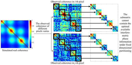
Figure 1.
The limitations of fixed-dimensional partitioning for the full-covariance matrix.
To overcome these limitations, an adaptive submatrix partitioning strategy is proposed, guided by prior coherence information. The procedure begins with extracting the coherence matrix from the full-covariance matrix. Each element in the coherence matrix reflects the interferometric phase quality of a pair of SAR acquisitions, thus providing a direct measure of phase reliability. This value is used as prior information for submatrix partitioning.
where is the coherence matrix.
Based on characteristics of the study area, a temporal baseline threshold is defined, assuming that interferometric pairs with temporal baselines exceeding this threshold rarely exhibit phase information with coherence values above 0.1. The SAR image with a temporal baseline nearest to this threshold, denoted as Nmax, is selected as the upper bound for submatrix dimension. The phase information beyond this dimension cannot be considered beneficial for optimizing performance to a large extent.
where is the time interval from the 1-th scene image to the N-th scene image, i.e., the temporal baseline, and is the temporal baseline threshold. Meanwhile, the minimum submatrix size is constrained to Nmin = 5.
Subsequently, an initial submatrix of size Nmax × N is extracted. The average coherence across each of the same temporal baselines is calculated along the diagonal vectors:
where is the average coherence vector of size 1 × N.
Since coherence typically decreases with increasing temporal baseline in theory, generally shows a declining trend. Even the seasonal coherence model may exhibit an indirect local declining trend. Therefore, a coherence stability detection method based on persistent exceedance detection analysis is adopted to detect a continuous threshold stable segment, that is, identify the stable interval above a coherence threshold, which is set to 0.2, from the average coherence vector. The farthest position within this interval is denoted as Nk. The dimension of the first submatrix patch can be defined as:
To ensure smooth transitions between optimized phase subsequences, a patch overlap criterion is introduced. The overlap ratio is set to 30%. Additionally, the minimum overlapping dimension is set to 2 to ensure effective repeated observations for subsequent adjustment correction, expressed as,
where Nolap is the overlapping dimension, ⌊⌋ is the rounding operation.
Following the construction of the first covariance submatrix patch of dimension Np1 × Np1, the overlapping dimension between the first and second submatrices is defined as Nolap based on the above overlap criterion for submatrices. Guided by the sequential extraction principle, the starting pixel position of the second submatrix is determined as (Np1-Nolap + 1, Np1-Nolap + 1). From this position, an initial covariance submatrix with dimension Nmax × (N-Np1 + Nolap) is extracted. The dimension of the second submatrix, Np2, is then estimated by applying the same procedures used for the first patch, namely average coherence vector estimation and coherence stability detection. Furthermore, the same processes, including overlapping dimension estimation, initial pixel position for extraction determination, initial submatrix construction, and submatrix dimension estimation, are repeated iteratively for all subsequent patches. Through this recursive process, the full-covariance matrix with dimension N × N is adaptively partitioned into multiple covariance submatrix patches with variable dimensions. The detailed processes of adaptive partitioning of the covariance matrix are shown in Figure 2.
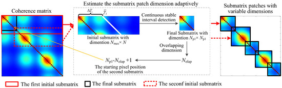
Figure 2.
The diagram of adaptive partitioning of the full-covariance matrix.
3.2. Subsequence Phase Optimization and Adjustment Correction
Once covariance submatrices with different dimensions are obtained adaptively, local phase optimization is performed sequentially. The advanced studies indicate that the choice of the local optimization model has little effect on the overall sequential framework [27]. Therefore, any current phase optimization model can be adopted for local optimization processing. In this study, two representative methods are employed: EMI and true maximum likelihood estimation (TMLE) [30].
The EMI method modifies the standard MLE optimization model by introducing correction factors. This adjustment retains the strong performance of MLE while mitigating the inefficiency of nonlinear solvers. The optimized phase is obtained by the eigenvector associated with the smallest eigenvalue of .
The TMLE method derives a phase optimization model that couples coherence and phase by simultaneously considering the maximum likelihood estimator of coherence and phase, achieving true maximum likelihood estimation of phase. Under the assumption of a complex circular Gaussian distribution, the logarithmic function of the probability density function corresponding to the phase is expressed as:
where ln() is the logarithmic operation, det() is the determinant operation, is the true coherence matrix, is the SLC phase vector, is the complex phase matrix containing the true phase sequence, is the transpose operation, and diag() is the diagonal matrix operation. Combining maximum likelihood estimation, the maximum likelihood estimator of coherence and phase can be derived, respectively.
where Re() is the real part operation.
TMLE fully considers the maximum likelihood estimator of the coherence matrix, rather than directly using the approximate value of . Therefore, the likelihood function constructed by this method strictly follows the statistical model and can truly represent the maximum likelihood value of the given solution, without being affected by the poor estimation of the sample coherence matrix, and has better optimization performance. However, its reliance on nonlinear optimization makes it more computationally demanding.
For each submatrix, the chosen optimization model yields an optimized phase subsequence. Given that the submatrix patch overlap process is employed to improve continuity between optimized phase subsequences, the optimized phase subsequence can be expressed as,
Subsequently, the compensated optimized phase subsequence is obtained by performing data compression and reference compensation. However, due to the overlap criterion introduced in the adaptive partitioning process, different subsequences share common elements. To ensure phase continuity across submatrices, an adjustment correction procedure is proposed.
Let the phase of common elements in the overlapping region of the i-th and j-th compensated optimized phase subsequences be denoted as and , respectively. According to the theory of data adjustment, the final optimized phase at the common element can be expressed in the form of observation equations,
These equations can be combined and transformed into matrix form, that is,
where is the design matrix corresponding to the observations of the compensated optimized phase subsequences, represents residuals. The corrected phase at the common element is derived by solving the above equation using the weighted least squares estimator.
where P denotes the weight matrix, and are the i-th and j-th subsequence. In accordance with the principle of error propagation, a smaller weight is assigned to a phase originating from a later subsequence. This design reduces the influence of accumulated uncertainty across the sequential processing chain.
Once the corrected phase of the overlapping element is obtained, the adjustment continues by calculating the mean residual between consecutive subsequences. Specifically, using the previous subsequence as a reference, the mean residual of the latter subsequence is then propagated to the latter subsequence as a correction term, expressed as,
The final corrected optimized phase subsequence can then be obtained,
By iteratively applying this adjustment to all compensated subsequences, the entire set of corrected subsequences is obtained. The final optimized phase is then estimated by concatenating these corrected subsequences in order and eliminating redundant overlapping phases. The procedure ensures the global continuity of the final optimized phase, thereby improving the stability and accuracy of the proposed adaptive sequential phase optimization framework.
3.3. Overall Framework
The overall process of the proposed adaptive sequential phase optimization algorithm is as shown in Algorithm 1.
| Algorithm 1. Pseudocode of the proposed adaptive sequential phase optimization algorithm |
| Input data: Time series SLC data (N scenes) |
for i-th pixel (∈ image) do
|
| Output data: Optimized time series SLC data |
4. Experimental Analysis of Simulated Data
To evaluate the effectiveness of the proposed adaptive sequential phase optimization method (AdSeq), the simulation-based experiments were conducted. The performance of AdSeq was compared against state-of-the-art phase optimization methods: EMI, TMLE, and Sequential (Seq). Moreover, to further investigate the influence of local optimization models, AdSeq was tested with both EMI and TMLE as local optimization models, referred to as AdSeq + EMI and AdSeq + TMLE, respectively.
The complex coherence between the m-th and n-th SAR acquisitions is defined as,
where denotes the general coherence model, is the temporal baseline, is the radar wavelength, and represent short-term and long-term coherence, is the temporal decorrelation constant, and v is the deformation rate and the linear deformation rate is adopted. represents the short-term coherence model and corresponds to the long-term coherence model. For the seasonal coherence model, the coherence is further defined as:
where and are the temporal baselines relative to the first image, respectively.
The long-term, short-term, and seasonal coherence models were adopted for experiments. The deformation rate was set at 4 mm/a, and other parameters were set as shown in Table 1. Based on this setup, 50 images with 100 statistically homogeneous pixels were simulated. The generating coherence and phase are shown in Figure 3.

Table 1.
Parameter setting of the coherence model.
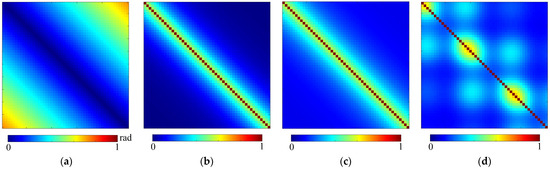
Figure 3.
Simulated datasets. (a) Phase; (b) Short-term coherence; (c) Long-term coherence; (d) Seasonal coherence.
4.1. Optimization Performance Analysis
Phase optimization was then performed on the simulated datasets with EMI, TMLE, Seq, AdSeq + EMI, and AdSeq + TMLE methods. The submatrix dimension was fixed at 10 in the Seq method. Optimization accuracy was quantified using the root mean square error (RMSE), which is shown in Figure 4.
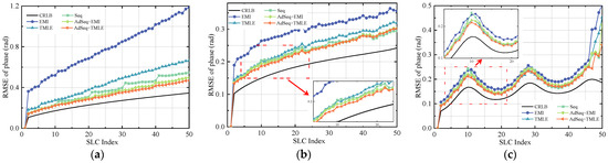
Figure 4.
The optimized phase results of simulated datasets. (a) Short-term coherence; (b) Long-term coherence; (c) Seasonal coherence.
For the experimental results of short-term coherence shown in Figure 4a, the Cramér–Rao lower bound (CRLB) of the optimized phase RMSE increases approximately linearly with temporal baseline, reaching about 0.35 rad at the last acquisition. The CRLB represents the theoretical minimum variance and highest accuracy of the optimized phase estimator, and the closer the RMSE value is to it, the better the optimization performance. EMI yields the worst performance, with a mean RMSE of about 0.78 rad and a standard deviation of about 0.24 rad, reaching as high as 1.18 rad. TMLE improves the performance significantly, with a mean RMSE of about 0.44 rad and a standard deviation of about 0.15 rad. This is mainly thanks to its joint modeling for the maximum likelihood estimator of phase and coherence and the regularization processing of the coherence matrix. Seq achieves a lower mean RMSE with about 0.37 rad and standard deviation with about 0.12 rad than EMI and TMLE. However, the optimized phase obtained by Seq suffers from sharp jumps due to discontinuities at optimized phase sequence boundaries. The proposed AdSeq method yields the lowest RMSE and best optimization performance compared to EMI, TMLE, and Seq, resolving the discontinuity issue of Seq and achieving the best phase continuity. Regarding the analysis of different local phase optimization models in AdSeq, AdSeq + EMI has a mean RMSE of about 0.34 rad and a standard deviation of about 0.10 rad, while AdSeq + TMLE performs slightly better, with a mean RMSE of about 0.32 rad and a standard deviation of about 0.09 rad. The slight difference between AdSeq + EMI and AdSeq + TMLE experimental results confirms that while TMLE is superior to EMI, the AdSeq framework reduces the sensitivity to the choice of local optimization model.
According to experimental results analysis under the long-term coherence model, as illustrated in Figure 4b, the coherence maintains a minimum level of approximately 0.1 even when the temporal baseline becomes considerably extended. As a result, the CRLB of the RMSE for the optimized phase at the longest temporal baseline is only 0.24 rad. This characteristic indicates that, in contrast to the short-term coherence model, the long-term model provides a more stable interferometric environment, allowing all phase optimization methods to achieve enhanced performance. Among them, EMI exhibits the most noticeable improvement, with the maximum RMSE of the optimized phase reaching approximately 0.36 rad and the mean value about 0.30 rad. However, its overall optimization performance still remains the poorest compared to the other methods. TMLE performs better than EMI, yet the optimization performance decreases markedly under long temporal baselines compared to the Seq and AdSeq methods. And, the mean RMSE corresponding to TMLE stabilizes about 0.25 rad. In contrast, Seq, AdSeq + EMI, and AdSeq + TMLE methods deliver similar optimization results, all significantly outperforming EMI and TMLE. Their corresponding mean RMSE are about 0.24 rad, 0.24 rad, and 0.23 rad, respectively. A closer inspection of the locally enlarged region reveals that at shorter temporal baselines, the optimization performance of AdSeq is slightly superior to that of Seq, especially the AdSeq + TMLE method. As the temporal baseline increases, the performances of Seq, AdSeq + EMI, and AdSeq + TMLE gradually converge, exhibiting nearly identical accuracy levels.
As illustrated in Figure 4c, the coherence of the seasonal coherence model remains at least 0.1 even under long temporal baselines, and maintains relatively high values within specific seasonal periods. Consequently, the CRLB of RMSE also exhibits periodic variations corresponding to the periodic coherence changes over the temporal baseline. Owing to the periodically high coherence, all tested methods demonstrate improved performance and exhibit similar periodic trends. However, at the longest temporal baseline, the optimization performance of all methods deteriorates significantly, with EMI performing the worst, followed by the TMLE. Specifically, EMI consistently yields the highest RMSE with a mean value of about 0.22 rad, indicating the poorest performance. TMLE, Seq, and AdSeq methods demonstrate similar optimization performance, and their differences are not visually significant. Based on the locally enlarged region under shorter temporal baselines, AdSeq + TMLE shows slightly better optimization performance. According to statistical analysis, the mean RMSE of TMLE, Seq, AdSeq + EMI, and AdSeq + TMLE methods are approximately 0.196 rad, 0.193 rad, 0.194 rad, and 0.187 rad, respectively, further indicating that the proposed AdSeq achieves relatively better optimization performance.
4.2. Computational Efficiency Analysis
Based on the above limited simulated dataset, the computational efficiency of different phase optimization methods is evaluated, as summarized in Table 2. The results show that the proposed AdSeq incurs a modest computational overhead due to the inclusion of adaptive dimension estimation and overlapping adjustment correction procedures. Consequently, the computation time of AdSeq + EMI is slightly higher than that of EMI and Seq, yet remains substantially lower than that of the TMLE. In addition, because TMLE relies on a computationally intensive nonlinear optimization strategy, AdSeq + TMLE exhibits a longer runtime than AdSeq + EMI, though still less than that of standalone TMLE.
Table 2.
Computation time of different methods.
Importantly, the efficiency advantage of Seq-type methods extends beyond the experimental setting with a fixed dataset. These methods are inherently scalable: when new SAR images are incorporated, only the newly added segments require local optimization and compensation, avoiding the need for full re-optimization of the entire dataset as required by EMI. This characteristic makes Seq-type strategies especially suitable for long-term monitoring scenarios and continuously growing InSAR archives.
5. Experimental Analysis of Real Data
To further verify the effectiveness and reliability of the proposed AdSeq, a real data experiment was conducted using Sentinel-1A SAR images covering the Shilawusu Coal Mine in the Inner Mongolia Autonomous Region. A total of 34 ascending orbit SAR images acquired in Interferometric Wide Swath mode with VV polarization were collected, covering the period from January 2018 to March 2019. The temporal interval between adjacent images was 12 days. The coverage map of the study area is shown in Figure 5.
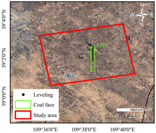
Figure 5.
The study area coverage diagram of the real dataset.
Based on the conclusions drawn from the simulated dataset experiments, AdSeq in this experiment was implemented using the EMI local phase optimization model to balance computational efficiency and optimization performance. Seq was configured with a fixed submatrix dimension of 10.
5.1. Qualitative Analysis of Optimized SLC Interferometric Phase
To qualitatively evaluate the optimization performance, a representative interferometric pair with a temporal baseline of 180 days was selected, corresponding to a period of pronounced ground deformation in the mining area. The optimized interferometric phase after removing flat-earth and topographic phase processed by EMI, TMLE, Seq, and AdSeq methods is illustrated in Figure 6.
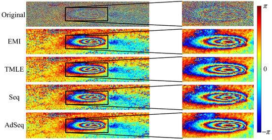
Figure 6.
The optimized interferometric phase obtained by different optimization methods.
It can be found that the original long temporal baseline interferogram exhibits significant phase noise, which obscures deformation signals. Although an irregular elliptical deformation field can still be vaguely discerned in the central region, the pervasive noise considerably limits the accuracy of the deformation interpretation. After phase optimization processing, all methods demonstrate a noticeable reduction in phase noise and a smoother phase structure. Specifically, EMI, TMLE, and Seq provide similar noise suppression performance but retain significant residual noise in the left and upper-right areas of the image. In contrast, AdSeq more effectively reduces phase noise, producing the smoothest interferometric phase among all methods, which indicates that AdSeq achieves superior noise suppression performance. Regarding fringe preservation within the deformation region, locally enlarged analyses show that the first three methods all suffer from notable fringe discontinuities and loss of phase information in areas with dense fringes. Seq is the most severe, followed by EMI, while TMLE performs relatively better. However, the proposed AdSeq achieves a more effective and smoother restoration of the phase fringes, ensuring better phase continuity and preservation of deformation details and greatly facilitating accurate interpretation of deformation.
5.2. Quantitative Analysis of Optimized SLC Interferometric Phase
To more intuitively compare the optimized interferometric phase quality obtained by different phase optimization methods, the number of residues (NR), sum of the phase difference (SPD), and phase standard deviation (PSD) were selected as the quantitative evaluation indicators. The NR reflects the number of phase residues; a smaller NR value indicates higher interferometric phase quality. Similarly, both SPD and PSD characterize the smoothness of the interferometric phase; smaller values imply a smoother phase and stronger noise suppression ability. The percentage improvement of the optimized interferometric phase relative to the original interferometric phase under each evaluation indicator was calculated, and the mean and standard deviation of these improvements are summarized as shown in Figure 7.
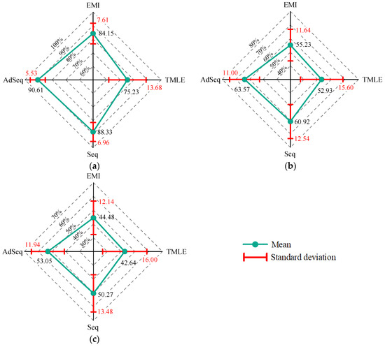
Figure 7.
The mean and standard deviation of percentage improvement in interferometric phase evaluation indicators. (a) NR; (b) SPD; (c) PSD.
In terms of NR, TMLE yields a relatively weak NR suppression rate of approximately 75.23%, while EMI reaches about 84.15%, showing a better noise suppression effect than TMLE. This slight deviation from the simulation-based results likely arises from the non-convergence of nonlinear optimization caused by limited iterations and suboptimal initializations in TMLE. Seq further improves the NR suppression rate to 88.33%, outperforming EMI and TMLE. Remarkably, AdSeq achieves the highest mean NR suppression rate of 90.61%, exceeding Seq, EMI, and TMLE by 2.28%, 6.46%, and 15.38%, respectively, thus demonstrating the best noise suppression performance. Furthermore, AdSeq exhibits the lowest standard deviation, only 5.53%, which is 1.43%, 2.08%, and 8.15% lower than those of Seq, EMI, and TMLE, respectively. This indicates that AdSeq maintains the strong stability and robustness across different temporal baselines.
Regarding the SPD, TMLE exhibits the poorest phase smoothness, with a mean percentage improvement of only 52.93%, followed by EMI at 55.23%. However, AdSeq reaches the highest mean percentage improvement of about 63.57%, outperforming Seq, EMI, and TMLE by 2.65%, 8.34%, and 10.64%, respectively. And, AdSeq achieves the lowest standard deviation of percentage improvement, only about 11%. These results clearly demonstrate that AdSeq yields the best phase smoothness. Similarly, for the PSD, AdSeq again achieves the highest mean percentage improvement of about 53.05%, surpassing Seq, EMI, and TMLE by 2.78%, 8.57%, and 10.41%, respectively, while maintaining the lowest standard deviation, reduced by 1.54%, 0.20%, and 4.06%, respectively. Overall, the proposed AdSeq produces the best phase smoothness and noise robustness in each indicator, demonstrating the best phase optimization performance.
5.3. Temporal Coherence Analysis
To comprehensively assess the impact of phase optimization on deformation interpretation, a temporal coherence analysis was performed on the optimized phases obtained by different methods. Temporal coherence serves as a critical indicator for identifying DS candidates, fundamentally influencing the density and reliability of monitoring points in subsequent DSInSAR processing.
It is important to note that, in the classical definition of temporal coherence, the temporal coherence of each pixel is calculated using all elements of the phase observation matrix, as shown in Figure 3a. This definition remains valid for EMI and TMLE methods, as both utilize the entire observation phase matrix as input. However, Seq and AdSeq optimization models operate on partial submatrices of the phase observation matrix, as illustrated in Figure 1 and Figure 2, rather than the full matrix. Consequently, directly applying the conventional temporal coherence formula may lead to a biased estimation that does not truly reflect their optimization performance. Moreover, if the actual submatrices used by each optimization model are adopted for temporal coherence computation, the results across methods would lose reference consistency, making direct comparison impossible. Therefore, the local phase submatrix with fixed dimension, smaller than the Seq submatrix dimension, is introduced as the computational unit for temporal coherence to ensure fair evaluation. The submatrix dimension is set to 7, and the modified temporal coherence is defined as,
where Np is the submatrix dimension, Ns is the number of submatrix patches divided by the submatrix dimension.
As illustrated in Figure 8, TMLE yields the poorest overall temporal coherence, with many low-coherence values distributed along the left and right regions of the study area. EMI performs slightly better. While Seq and AdSeq achieve similar temporal coherence and are significantly better than EMI and TMLE. Local analysis of the left and right regions further reveals that AdSeq performs slightly better than Seq, though the difference is subtle.
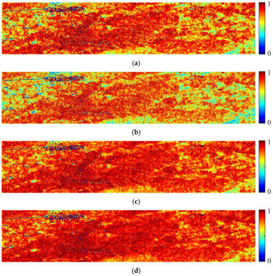
Figure 8.
The temporal coherence. (a) EMI; (b) TMLE; (c) Seq; (d) AdSeq.
A statistical evaluation of the temporal coherence distributions was conducted to further accurately assess these observations, as shown in Figure 9. TMLE exhibits the lowest density of high-coherence pixels, with a peak of coherence density around 0.8. The proportion of pixels with temporal coherence above 0.8 for AdSeq, Seq, EMI, and TMLE is approximately 73.11%, 63.77%, 49.16%, and 35.16%, respectively. However, the peak of coherence density corresponding to the other three methods appears near 0.9. Using 0.9 as a threshold, the proportion of pixels with temporal coherence greater than 0.9 for AdSeq reaches 35.07%, which is approximately 8.01%, 16.28%, and 23.20% higher than those of Seq, EMI, and TMLE, respectively. These results further demonstrate that the proposed AdSeq achieves the best optimization performance. In addition, the higher proportion of pixels with large temporal coherence obtained by AdSeq directly contributes to a denser distribution of DS candidate points. This allows many high signal-to-noise ratio phases to be selected for deformation interpretation, thereby improving the precision and reliability of deformation monitoring.
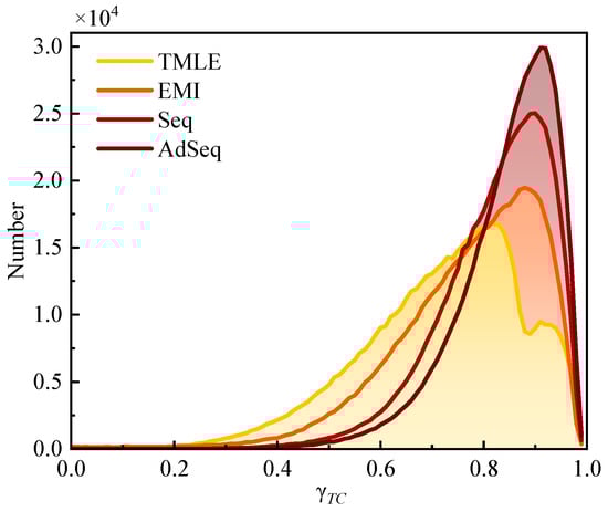
Figure 9.
The statistical analysis of temporal coherence.
5.4. Deformation Monitoring Results Analysis
Based on the optimized phase obtained by different methods, a temporal coherence threshold of 0.85 was adopted to select DS candidate points for subsequent deformation information interpretation, and the final deformation monitoring products were generated. The optimization performance can be further effectively evaluated by comparing the impact of different optimization methods on the final deformation results, as shown in Figure 10.
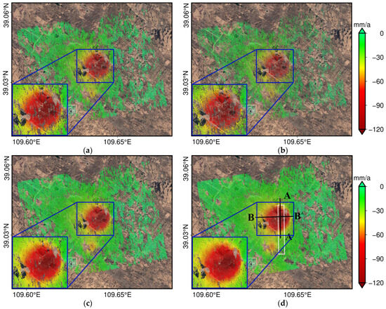
Figure 10.
The deformation rate results obtained by different methods. (a) EMI; (b) TMLE; (c) Seq; (d) AdSeq.
Deformation rate results derived from the integrated PS and DS processing exhibit extensive spatial coverage of monitoring points across the study area, providing a solid basis for accurate deformation interpretation. However, significant differences in monitoring point density are evident among the deformation results obtained using different phase optimization methods. Specifically, TMLE produces the sparsest monitoring points, with approximately 113,090, corresponding to a density of about 3635 pixels/km2. EMI performed moderately better, generating around 177,323 monitoring points, corresponding to 5700 pixels/km2. The limited density observed for both TMLE and EMI is attributed to their weaker phase optimization capability, which fails to maintain stable and reliable phases over long temporal baselines, leading to fewer pixels being selected as final DS points. In contrast, Seq significantly increases the number of monitoring points to 275,248, corresponding to about 8847 pixels/km2, notably superior to TMLE and EMI deformation results. The proposed AdSeq, however, achieves the highest monitoring point density, with 333,256 monitoring points, corresponding to about 10,712 pixels/km2. Compared to Seq, EMI, and TMLE, the monitoring point density increases by approximately 21.07%, 87.94%, and 194.68%, respectively. The deformation results obtained by AdSeq reveal more detailed subsidence information within the study area, particularly in regions with a large deformation gradient. Spatially, the detected deformation field corresponds closely to the active coal extraction zone of the 1201 working face in the Shilawusu Coal Mine, indicating strong geophysical consistency between observed deformation and mining activities.
To further investigate the deformation characteristics of the study area, two cross-sectional profiles, A–A′ and B–B′, were established along the strike and dip directions of the 1201 working face, as shown in Figure 10d. The deformation rate and time series deformation along these profiles were extracted and analyzed, as illustrated in Figure 11.
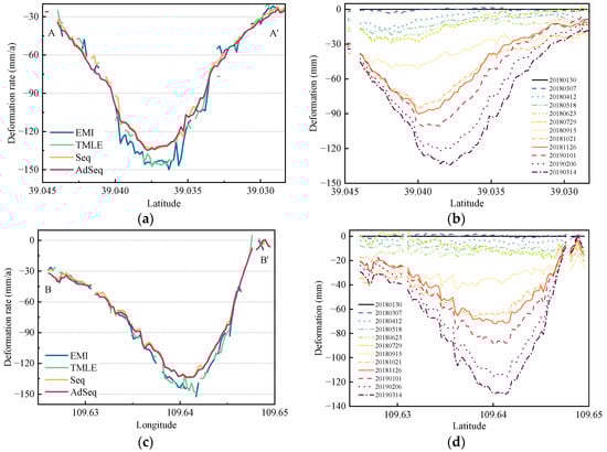
Figure 11.
The deformation rates and time series deformation of profile lines. (a,c) Deformation rates; (b,d) Time series deformation; (a,b) Profile lines A–A′; (c,d) Profile lines B–B′.
According to the deformation results at profile line A–A′, TMLE retains only about 60% of valid data, followed by EMI with approximately 74%. The sparse distribution of monitoring points severely limits the interpretability of deformation behavior in the mining area. In contrast, Seq and AdSeq achieve much higher valid data coverage along the profile, reaching about 88% and 98%, respectively, consistent with the conclusion of monitoring density analysis presented earlier. Furthermore, the deformation rate results derived from AdSeq and Seq are similar, and the maximum subsidence rates are approximately 134.77 mm/a and 134.35 mm/a, respectively. However, EMI and TMLE produce the larger maximum subsidence rates of about 149.90 mm/a and 146.50 mm/a, indicating an apparent overestimation of deformation. This overestimation is primarily attributed to the limited number of valid monitoring points, which restricts the reliability of the deformation interpretation.
The time series deformation results derived from AdSeq were further extracted to capture the temporal evolution of the subsidence process. To enhance readability, the results were temporally resampled to an average interval of 36 days. The time series deformation along profile A–A′ shows that from 30 January 2018 to 29 July 2018, the ground experienced slow subsidence, with a maximum displacement of about 29.42 mm over 180 days. Subsequently, the deformation rate increased sharply from 29 July to 21 October, 2018, with a cumulative subsidence of 58.05 mm in 84 days. Between 21 October and 26 November 2018, the deformation rate slowed, but accelerated again between 26 November 2018 and 14 March 2019, reaching a maximum cumulative subsidence of 134.22 mm.
For profile B–B′, the maximum subsidence rate estimated by AdSeq and Seq are approximately 133.75 mm/a and 134.30 mm/a, respectively. However, EMI and TMLE yield larger maximum subsidence rates of 152.40 mm/a and 148.76 mm/a, likely due to the same overestimation effect caused by low monitoring point density. Additionally, the temporal evolution of surface deformation along profile B–B′ is also largely consistent with that of profile A–A′.
5.5. Deformation Monitoring Accuracy Analysis
To rigorously evaluate the accuracy of deformation results derived from different phase optimization methods, high-precision leveling data acquired from the 1201 working face, as shown in Figure 5, were employed for comparative analysis. For consistency, the initial leveling survey date was taken as the temporal reference, and a stable leveling point located in a non-deforming region was used as the spatial reference. For convenience of contrast, the DSInSAR-derived line-of-sight (LOS) deformation results were converted to the vertical direction, expressed as,
where , , , and are the LOS, vertical, east–west, and north–south deformations, respectively, is the incidence angle, is the heading angle. Noted that, due to the limitations of one look observation, deformations in the east–west and north–south directions are ignored in this experiment. Furthermore, the same temporal and spatial reference framework is calibrated to ensure direct comparability with leveling data.
Taking the maximum cumulative deformation observed during the leveling survey period as the reference, the difference between the deformation results obtained from different methods and the leveling data was statistically analyzed, as shown in Table 3. TMLE exhibits the most significant deviation, with an RMSE of 21.44 mm and a mean difference of −14.49 mm, indicating the poorest monitoring accuracy. EMI achieves slightly better results, with an RMSE of 19.11 mm and a mean difference of −11.70 mm. Seq further improves monitoring accuracy, yielding an RMSE of 18.34 mm and a mean difference of −10.62 mm. However, the proposed AdSeq achieves the lowest RMSE of 16.49 mm, corresponding to improvements of 10.09%, 13.71%, and 23.09% over the Seq, EMI, and TMLE methods, respectively. Moreover, AdSeq maintains the lowest mean of −7.68 mm and standard deviation of about 14.27 mm. These results all confirm its superior deformation monitoring accuracy.
Table 3.
Statistics of deformation differences.
To comprehensively evaluate the consistency between leveling data and DSInSAR deformation results, Pearson correlation analyses were performed across all monitoring epochs and observation points. As shown in Figure 12, the Pearson correlation coefficient between the leveling data and the TMLE-based deformation results is the lowest, at about 0.934, followed by EMI at 0.938. Seq achieves a higher correlation of 0.942, while the proposed AdSeq maintains the strongest agreement with the leveling data, reaching 0.943, further demonstrating its superior deformation monitoring accuracy.
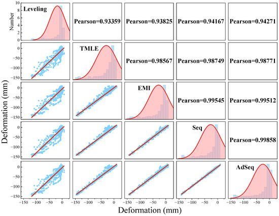
Figure 12.
Correlation of deformation results.
Additionally, inter-comparisons between deformation results from different methods reveal that TMLE exhibits the lowest absolute accuracy and the weakest correlations with other methods, with only about 0.987. The EMI result shows higher consistency with those from Seq and AdSeq, with correlation coefficients around 0.995. Notably, the Seq and AdSeq deformation results are highly consistent, with a correlation coefficient as high as 0.998, further highlighting the strong reliability and stability of the AdSeq phase optimization approach.
6. Discussion
As described in the previous methods and experiments, the proposed AdSeq can effectively address the problem of phase discontinuity in phase subsequences of traditional Seq. However, its improvement level needs further in-depth and detailed exploration. Therefore, more experiments were conducted under the short-term coherence model to further analyze the differences in phase discontinuity between the proposed AdSeq and the conventional Seq. Meanwhile, the influence of submatrix dimension on the optimization performance of Seq-type algorithms is evaluated. Specifically, the submatrix dimensions were set to 14, 10, and 6, respectively, and the optimization results are shown in Figure 13.
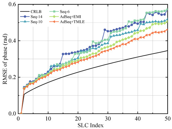
Figure 13.
The optimized phase results under different submatrix dimensions.
The analysis of the results reveals that, regardless of the selected submatrix dimension, Seq consistently exhibits noticeable phase jumps between adjacent optimized phase subsequences. This phenomenon implies that the data compensation strategy adopted by Seq fails to achieve phase continuity across subsequences. Furthermore, when the submatrix dimension is set to 14 and 6, the mean RMSEs are approximately 0.383 rad and 0.377 rad, respectively, showing similar performance. A moderate improvement is obtained when the submatrix dimension is 10, yielding a slightly lower mean RMSE with 0.357 rad. Overall, the comparative analysis confirms that the submatrix dimension in Seq exhibits no significant correlation with the phase optimization performance. However, discontinuities between optimized phase subsequences persist in all cases. In contrast, the proposed AdSeq effectively addresses the deficiency of reference compensation in the traditional Seq by introducing an adaptive patch overlapping mechanism and a common element adjustment procedure. This significantly enhances the continuity between optimized phase subsequences and yields the best overall phase optimization performance.
7. Conclusions
At present, the sequential phase optimization method has not sufficiently considered the spatiotemporal variability characteristics of pixels and the heterogeneity among pixels. This limitation results in unreasonable submatrix partitioning and poor continuity between phase subsequences, severely constraining the overall optimization performance. Therefore, an adaptive sequential phase optimization method that integrates coherence stability detection and adjustment correction is proposed in this paper. Specifically, the proposed method first employs a coherence stability detection mechanism to adaptively determine the dimension of covariance submatrices, ensuring that the partitioning process preserves the most stable and informative phase observations. A submatrix patch overlap strategy is then introduced to maintain continuity across neighboring subsets. Finally, a weighted least squares adjustment correction is developed to connect optimized phase subsequences, leading to a more continuous and robust phase optimization outcome.
Simulation experiments demonstrate that the proposed AdSeq consistently achieves the lowest RMSE under short-term, long-term, and Seasonal coherence models, confirming superior optimization performance. Moreover, submatrix dimensional setting experiments of sequential-type methods indicate that it is difficult to establish a clear relationship between dimensional settings and optimization performance. Nevertheless, conventional sequential methods under any dimension consistently suffer from significant phase discontinuity, whereas the proposed AdSeq effectively mitigates this problem and further enhances phase optimization performance.
Real data experiments over the Shilawusu Coal Mine show that the proposed AdSeq significantly improves the quality of optimized interferometric phase, and the density of deformation monitoring points reaches 10,712 pixels/km2, an improvement of more than 21.07% compared with traditional methods. Moreover, the deformation monitoring accuracy reaches 16.49 mm, corresponding to improvements of 10.09%, 13.71%, and 23.09% over the Seq, EMI, and TMLE methods, respectively. These results collectively confirm that the proposed AdSeq achieves superior phase optimization performance and deformation monitoring accuracy.
Author Contributions
Conceptualization, S.L.; methodology, S.L. and Y.G.; software, Y.G. and H.B.; validation, Y.M., Y.Y. and Q.C.; formal analysis, S.L. and W.D.; investigation, Y.G. and N.Z.; resources, W.D., Y.Y. and B.J.; writing—original draft preparation, S.L.; writing—review and editing, S.L. and Y.G.; visualization, H.B. and Y.Y.; supervision, Y.M. and B.J.; project administration, N.Z.; funding acquisition, S.L., Y.G. and N.Z. All authors have read and agreed to the published version of the manuscript.
Funding
This research was funded by National Natural Science Foundation of China (grant number 42404047, U22A20569, and 42271460), Natural Science Foundation of Jiangsu Province (grant number BK20241671), Major Scientific and Technological Special Projects of Xinjiang Uygur Autonomous Region (grant number 2024A01002), Jiangsu Funding Program for Excellent Postdoctoral Talent (grant number 2023ZB277); and China Postdoctoral Science Foundation (grant number 2023M733743).
Data Availability Statement
The original contributions presented in this study are included in the article. Further inquiries can be directed to the corresponding author.
Acknowledgments
The authors would like to thank the European Space Agency for providing Sentinel-1 data and the editor and reviewers for their insightful comments.
Conflicts of Interest
Author Qiang Chen was employed by the company Yankuang Energy Group Company Limited Jining No.3 Coal Mine. The remaining authors declare that the research was conducted in the absence of any commercial or financial relationships that could be construed as a potential conflict of interest.
References
- Xiao, R.; Wang, X.; Jiang, M.; Yuan, S.; Li, Z.; Wu, Z.; Ferreira, V.; He, X. Decadal Earth observation-informed analysis of urban riverbank deformation: InSAR insights into soft ground dynamics in Nanjing, China. Int. J. Appl. Earth Obs. Geoinf. 2025, 144, 104868. [Google Scholar] [CrossRef]
- Wang, F.; Liu, Q.; Li, R.; Wang, S.; Wang, H.; Wang, J.; Ma, X.; Zhou, L.; Wang, Y. Surface Deformation Monitoring and Prediction of InSAR-Hybrid Deep Learning Model for Subsidence Funnels. Remote Sens. 2025, 17, 2972. [Google Scholar] [CrossRef]
- Zhou, Y.; Hao, G.; Qin, X.; Yi, F.; Tan, Z. A refined DS-InSAR technique for long-term deformation monitoring of low-coherence bridge groups. Eng. Struct. 2025, 335, 120335. [Google Scholar] [CrossRef]
- Feng, J.; Fan, H.; Yuan, Y.; Liu, Z. Enhanced Phase Optimization Using Spectral Radius Constraints and Weighted Eigenvalue Decomposition for Distributed Scatterer InSAR. Remote Sens. 2025, 17, 862. [Google Scholar] [CrossRef]
- Zhang, Y.; Zhao, F.; Wang, Y.; Ma, Z.; Zhang, L.; Wang, T.; Huo, W.; Zou, G. Interferometric Phase Optimization Based on Total Power Polarization Optimization and Nonlocal Phase Linking. IEEE Trans. Geosci. Remote Sens. 2025, 63, 1–15. [Google Scholar] [CrossRef]
- Ansari, H.; De Zan, F.; Parizzi, A. Study of systematic bias in measuring surface deformation with SAR interferometry. IEEE Trans. Geosci. Remote Sens. 2021, 59, 1285–1301. [Google Scholar] [CrossRef]
- Morishita, Y.; Lazecky, M.; Wright, T.; Weiss, J.; Elliott, J.; Hooper, A. LiCSBAS: An open-source InSAR time series analysis package integrated with the LiCSAR automated Sentinel-1 InSAR processor. Remote Sens. 2020, 12, 424. [Google Scholar] [CrossRef]
- Zhang, Z.; Yan, S.; Zhang, H.; Zhao, F. Nonlocal phase linking for distributed scatterer interferometry. IEEE Trans. Geosci. Remote Sens. 2024, 62, 5201913. [Google Scholar] [CrossRef]
- Li, S.; Zhang, S.; Li, T.; Gao, Y.; Zhou, X.; Chen, Q.; Zhang, X.; Yang, C. An adaptive weighted phase optimization algorithm based on the sigmoid model for distributed scatterers. Remote Sens. 2021, 13, 3253. [Google Scholar] [CrossRef]
- Chen, B.; Liu, N.; Yu, H.; Zhao, F.; Zhu, C.; Zhang, L.; Liu, Z. TSO-PL: A Novel Phase Linking Method for DS InSAR Based on a Two-Step Strategy to Optimize the Sample Coherence Matrix. IEEE Trans. Geosci. Remote Sens. 2025, 63, 1–19. [Google Scholar] [CrossRef]
- Eppler, J.; Rabus, B.T. Adapting InSAR phase linking for seasonally snow-covered terrain. IEEE Trans. Geosci. Remote Sens. 2022, 60, 4305313. [Google Scholar] [CrossRef]
- Biessel, R.; Zwieback, S. An intensity triplet for prediction and correction of systematic InSAR closure phases. TechRxiv 2023. [Google Scholar] [CrossRef]
- Zhou, D.; Zhao, Z. Optimal algorithm for distributed scatterer InSAR phase estimation based on cross-correlation complex coherence matrix. Int. J. Appl. Earth Obs. Geoinf. 2024, 134, 104214. [Google Scholar] [CrossRef]
- Liang, H.; Zhang, L.; Li, X.; Wu, J. Coherence bias mitigation through regularized tapered coherence matrix for phase linking in decorrelated environments. ISPRS J. Photogramm. Remote Sens. 2024, 215, 369–382. [Google Scholar] [CrossRef]
- Zwieback, S. Cheap, valid regularizers for improved interferometric phase linking. IEEE Geosci. Remote Sens. Lett. 2022, 19, 4512704. [Google Scholar] [CrossRef]
- Shen, P.; Wang, C.; An, B. AdpPL: An adaptive phase linking-based distributed scatterer interferometry with emphasis on interferometric pair selection optimization and adaptive regularization. Remote Sens. Environ. 2023, 295, 113687. [Google Scholar] [CrossRef]
- Gao, Z.; He, X.; Ma, Z.; Wei, S.; Xiong, J.; Aoki, Y. Distributed Scatterer Interferometry for Fast Decorrelation Scenarios Based on Sparsity Regularization. IEEE Trans. Geosci. Remote Sens. 2024, 62, 1–14. [Google Scholar] [CrossRef]
- Zhao, C.; Yu, H.; Jiang, M.; Cao, J. A hybrid approach for high-precision phase estimation in distributed scatterer interferometry. IEEE Trans. Geosci. Remote Sens. 2024, 62, 5202416. [Google Scholar] [CrossRef]
- Ansari, H.; De Zan, F.; Bamler, R. Sequential estimator: Toward efficient InSAR time series analysis. IEEE Trans. Geosci. Remote Sens. 2017, 55, 5637–5652. [Google Scholar] [CrossRef]
- Mirzaee, S.; Amelung, F.; Fattahi, H. Non-linear phase linking using joined distributed and persistent scatterers. Comput. Geosci. 2023, 171, 105291. [Google Scholar] [CrossRef]
- Ao, M.; Wei, L.; Liao, M.; Zhang, L.; Dong, J.; Liu, S. Incremental multi temporal InSAR analysis via recursive sequential estimator for long-term landslide deformation monitoring. ISPRS J. Photogramm. Remote Sens. 2024, 215, 313–330. [Google Scholar] [CrossRef]
- Wang, G.; Li, Z.; Gao, H.; Hu, J.; Jiang, M.; Ren, P.; Zhang, J. Adaptive sequential estimator for InSAR time series phase estimation. Int. J. Appl. Earth Obs. Geoinf. 2025, 139, 104552. [Google Scholar] [CrossRef]
- Li, S.; Li, Z.; Gao, Y.; Zheng, N.; Yan, M.; Zhang, S.; Mao, Y.; Zhang, D. Multilevel Perception Sequential Phase Optimization for Distributed Scatterer InSAR Steep Deformation Monitoring. IEEE J. Sel. Top. Appl. Earth Obs. Remote Sens. 2025, 18, 28123–28136. [Google Scholar] [CrossRef]
- Wang, Y.; Luo, J.; Dong, J.; Mallorqui, J.J.; Liao, M.; Zhang, L.; Gong, J. Sequential polarimetric phase optimization algorithm for dynamic deformation monitoring of landslides. ISPRS J. Photogramm. Remote Sens. 2024, 218, 84–100. [Google Scholar] [CrossRef]
- El Hajjar, D.; Ginolhac, G.; Yan, Y.; Nabil El Korso, M. Sequential Covariance Fitting for InSAR Phase Linking. IEEE Trans. Geosci. Remote Sens. 2025, 63, 1–13. [Google Scholar] [CrossRef]
- Ning, C.; Hyongki, L.; Hahn Chul, J. Mathematical framework for phase-triangulation algorithms in distributed-scatterer interferometry. IEEE Geosci. Remote Sens. Lett. 2015, 12, 1838–1842. [Google Scholar] [CrossRef]
- Ansari, H.; De Zan, F.; Bamler, R. Efficient phase estimation for interferogram stacks. IEEE Trans. Geosci. Remote Sens. 2018, 56, 4109–4125. [Google Scholar] [CrossRef]
- Ferretti, A.; Fumagalli, A.; Novali, F.; Prati, C.; Rocca, F.; Rucci, A. A new algorithm for processing interferometric data-stacks: SqueeSAR. IEEE Trans. Geosci. Remote Sens. 2011, 49, 3460–3470. [Google Scholar] [CrossRef]
- Fornaro, G.; Verde, S.; Reale, D.; Pauciullo, A. CAESAR: An approach based on covariance matrix decomposition to improve multibaseline–multitemporal interferometric SAR processing. IEEE Trans. Geosci. Remote Sens. 2015, 53, 2050–2065. [Google Scholar] [CrossRef]
- Wang, C.; Wang, X.; Xu, Y.; Zhang, B.; Jiang, M.; Xiong, S.; Zhang, Q.; Li, W.; Li, Q. A new likelihood function for consistent phase series estimation in distributed scatterer interferometry. IEEE Trans. Geosci. Remote Sens. 2022, 60, 5227314. [Google Scholar] [CrossRef]
Disclaimer/Publisher’s Note: The statements, opinions and data contained in all publications are solely those of the individual author(s) and contributor(s) and not of MDPI and/or the editor(s). MDPI and/or the editor(s) disclaim responsibility for any injury to people or property resulting from any ideas, methods, instructions or products referred to in the content. |
© 2025 by the authors. Licensee MDPI, Basel, Switzerland. This article is an open access article distributed under the terms and conditions of the Creative Commons Attribution (CC BY) license (https://creativecommons.org/licenses/by/4.0/).