Article

Reconstructed SWHs Based on a Deep Learning Method and the Revealed Long-Term SWH Variance Characteristics During 1993–2024

1
State Key Laboratory for Climate System Predictions and Risk Management/Key Laboratory of Meteorological Disaster, Ministry of Education (KLME)/Collaborative Innovation Center on Forecast and Evaluation of Meteorological Disasters, Nanjing University of Information Science and Technology, Nanjing 210044, China
2
Key Laboratory of Space Ocean Remote Sensing and Application, Ministry of Natural Resources, Beijing 100081, China
3
School of Atmospheric Sciences, Nanjing University of Information Science and Technology, Nanjing 210044, China
4
School of Atmospheric Sciences, Sun Yat-Sen University and Southern Marine Science and Engineering Guangdong Laboratory (Zhuhai), Zhuhai 519082, China
5
National Climate Centre, Beijing 100081, China
6
National Satellite Ocean Application Service, Ministry of Natural Resources, Beijing 100081, China
7
Ministry of Education Key Laboratory for Earth System Modeling, Department of Earth System Science, Tsinghua University, Beijing 100084, China
*
Author to whom correspondence should be addressed.
Remote Sens. 2025, 17(23), 3802; https://doi.org/10.3390/rs17233802 (registering DOI)
Submission received: 22 September 2025 / Revised: 18 November 2025 / Accepted: 21 November 2025 / Published: 23 November 2025

Highlights

What are the main findings?
  • This study reconstructed daily long-term high-resolution 0.25° × 0.25° SWHs for 1993–2024 using a partial convolutional U-Net model with attention and residual blocks, altimeter swath-derived SWHs, and ERA5 SWHs.
  • Comparison between the daily reconstructed SWHs and ERA5 SWHs demonstrated enhanced accuracy for SWHs of >2.5 m (a range systematically underestimated in ERA5 SWHs).
What is the implication of the main finding?
  • ERA5 reanalysis data exhibit systematic underestimation of SWH in geographically complex straits and under high sea state conditions, but swath-derived SWH measurements from satellite altimeters can substantially enhance SWH accuracy in these regions.

Abstract

Long-term high-resolution spatial gridded altimeter-derived significant wave height (SWH) data with daily temporal resolution are fundamental to revealing the detailed processes through which weather systems influence the ocean. However, elucidation of those processes is hampered by the sparse coverage and narrow width of the swath of altimeter-derived SWHs. The core problem is how best to extract the spatial structure and then fill missing values around the daily swaths. Although recent developments in deep learning methods have improved the extraction of spatial features, progress regarding the reconstruction of gridded altimeter daily SWHs remains limited. This study reconstructed daily 0.25° × 0.25° gridded SWHs from 1993 to 2024 using a partial convolutional U-Net model with attention and residual blocks. Comparison between the daily reconstructed SWHs and ERA5 SWHs revealed that the reconstructed SWHs improved the accuracy for SWHs of >2.5 m, which are usually underestimated in the ERA5 data. The greatest differences were in China’s offshore waters, especially in the region of the Taiwan Strait and in waters influenced by the Huanghai Warm Current. This study highlights the importance of altimeter swath-derived SWHs in reconstructed gridded SWH datasets, particularly in complex straits and under high sea state conditions.

1. Introduction

Significant wave height (SWH), which is the average height of the highest one-third of waves, is an important parameter in oceanic engineering design and oceanographic research, reflecting the strength of air–sea interactions [1,2,3,4]. Unlike the huge numbers of observations acquired over land areas, measurements of SWH are rather sparse and usually acquired over long intervals [5]. The main sources of SWH data are buoy observations [6], ship-based measurements [7], and satellite remote sensing retrievals. Buoy observations are rare, particularly over the open ocean [8]. Ship-based measurements are characterized by limited spatiotemporal coverage outside of the main shipping channels, and few observations are taken when ships encounter a severe weather system [9]. Thus, satellite-based altimeter observations currently represent the primary source of SWH data over the open ocean because of their broader spatial coverage, relative stability, and ability to directly observe the sea state [10].
Nevertheless, given the limited operational lifespan of a space-based payload (usually only several years [11,12,13]), together with the narrow viewing swath of a nadir-looking altimeter (approximately several kilometers in the footprint), integration of multiple altimeter SWH sources is necessary. Several agencies expend considerable effort to integrate SWH data obtained by multiple altimeter missions [14]. These agencies include GlobWave (ftp://ftp.ifremer.fr, accessed on 20 November 2025), the Radar Altimeter Data System (http://rads.tudelft.nl, accessed on 20 November 2025, https://www.aviso.altimetry.fr, accessed on 20 November 2025), the China National Satellite Ocean Application Service (http://www.nsoas.org.cn/, accessed on 20 November 2025), the National Oceanic and Atmospheric Administration (https://www.noaa.gov/, accessed on 20 November 2025), the ESA Sea State Climate Change Initiative [15], and China’s National Climate Center (https://bcc.ncc-cma.net, accessed on 20 November 2025) [16]. Although altimeter SWHs are carefully calibrated and the quality of altimeter swath-derived SWHs is reasonably good [17], the large numbers of missing values around the altimeter swaths hamper the construction of high-resolution spatial gridded SWH data with daily temporal resolution [11]. Production of reliable daily altimeter-derived SWHs could support improved understanding of air–sea interactions under various weather processes and provide precise reference data for oceanic engineering design and numerical simulations.
The state-of-the-art daily numerical simulation of SWH is the European Centre for Medium-Range Weather Forecasts Fifth Generation Reanalysis (ERA5), which couples atmospheric, oceanic, and sea surface wave models [18]. Additionally, the high-quality ERA5 SWHs assimilate altimeter wave heights from satellite platforms such as ERS1/2 and Jason 1/2 [19]. The ERA5 SWHs are the output of numerical simulation, the basic principle of which is totally different to the SWHs obtained by altimeters. Under many types of complex sea conditions, such as in straits and in areas of strong air–sea interactions, the accuracy of a numerical model simulation is not as good as is usually expected. To improve the quality of simulated SWH data in areas of complex sea conditions, we must establish a daily gridded SWH dataset based on altimeter retrievals, the quality of which are relatively stable under high sea conditions.
The main obstacle to the construction of such a daily gridded SWH dataset is the sparse coverage and narrow width of altimeter swaths [20]. In recent years, despite considerable developments in deep learning methods for efficient extraction of spatial features and improvements in ERA5 SWHs, progress regarding the reconstruction of daily gridded SWHs with high horizontal resolution remains limited. Therefore, the objective of this study was to construct a daily gridded SWH climate dataset for China’s offshore waters using deep learning, ERA5 SWHs, and various altimeter swath-derived SWHs.
The remainder of this paper is arranged as follows. Section 2 outlines the validation data, ERA5 SWHs, and altimeter SWHs considered in the study and describes the deep learning method and workflow adopted. Section 3 presents validation results for the reconstructed SWHs against in situ observations and the outcomes of comparison with ERA5 SWHs in terms of spatial distribution, linear trend, and linear trend of the standard deviation (STD). The discussion is in Section 4, and the main conclusions are presented in Section 5.

2. Data and Methods

2.1. Data

2.1.1. ERA5 Significant Wave Height (SWH) Data

The background SWH data used for the deep learning method in this study were obtained from the ERA5 dataset (https://cds.climate.copernicus.eu/#!/home, accessed on 20 November 2025), which has been widely used in ocean-related climatic studies [21,22]. In this research, we used daily ERA5 SWH data with spatial resolution of 0.25° × 0.25°.

2.1.2. Applied Multisource Altimeter SWHs and Buoy Observations

This study also used SWH swath data extracted from two principal multisatellite altimeter datasets (Figure 1): one from GlobWave (1993–2016) called CERSAT (ftp://ftp.ifremer.fr/ifremer/cersat/products/swath/altimeters/waves/, accessed on 20 November 2025) [23] and the other called Sat6 (2015–2024) [16], which is composed of China–France Oceanography Satellite (CFOSAT) data from the China National Space Administration and the Centre National D’Etudes Spatiales [24], HY-2A [25], HY-2B [26], HY-2C [5], and HY-2D [27] data from the China National Satellite Ocean Application Service (https://osdds.nsoas.org.cn/OceanDynamics/, accessed on 20 November 2025), and Jason-3 data [28] from the Centre National D’Etudes Spatiales (ftp://ftp-access.aviso.altimetry.fr/geophysical-data-record/jason-3/, accessed on 20 November 2025). Additionally, buoy observations were obtained from the State Oceanic Administration of China (SOAC), the China Meteorology Administration (CMA), and the National Data Buoy Center (NDBC, https://www.ndbc.noaa.gov/, accessed on 20 November 2025).
Referring to the validation method [29], the statistical parameters used were the relative bias (RB), scattering index (SI), correlation coefficient (R), root mean square error (RMSE), and temporal STD for every grid box (Tstd), defined as follows:
R B = 100 % 1 N i = 1 N A i B i B ¯ ,
S I = 1 N i = 1 N A i A ¯ ( B i B ¯ ) 2 B ¯ ,
R = i = 1 N A i A ¯ ( B i B ¯ ) i = 1 N A i A ¯ 2 B i B ¯ 2 ,
R M S E = i = 1 n A i B i 2 n ,
T s t d = i = 1 n x i x ¯ 2 n 1 ,
where A i is the reconstruction or ERA5 SWH, B i is the buoy observation SWH, and N is the number of matched data pairs. In Equation (5), x is the SWH in one grid box from the reconstruction or ERA5, and n is the number of time series in the grid box.

2.1.3. Merging of the Two Main Multisource Altimeter SWHs Datasets

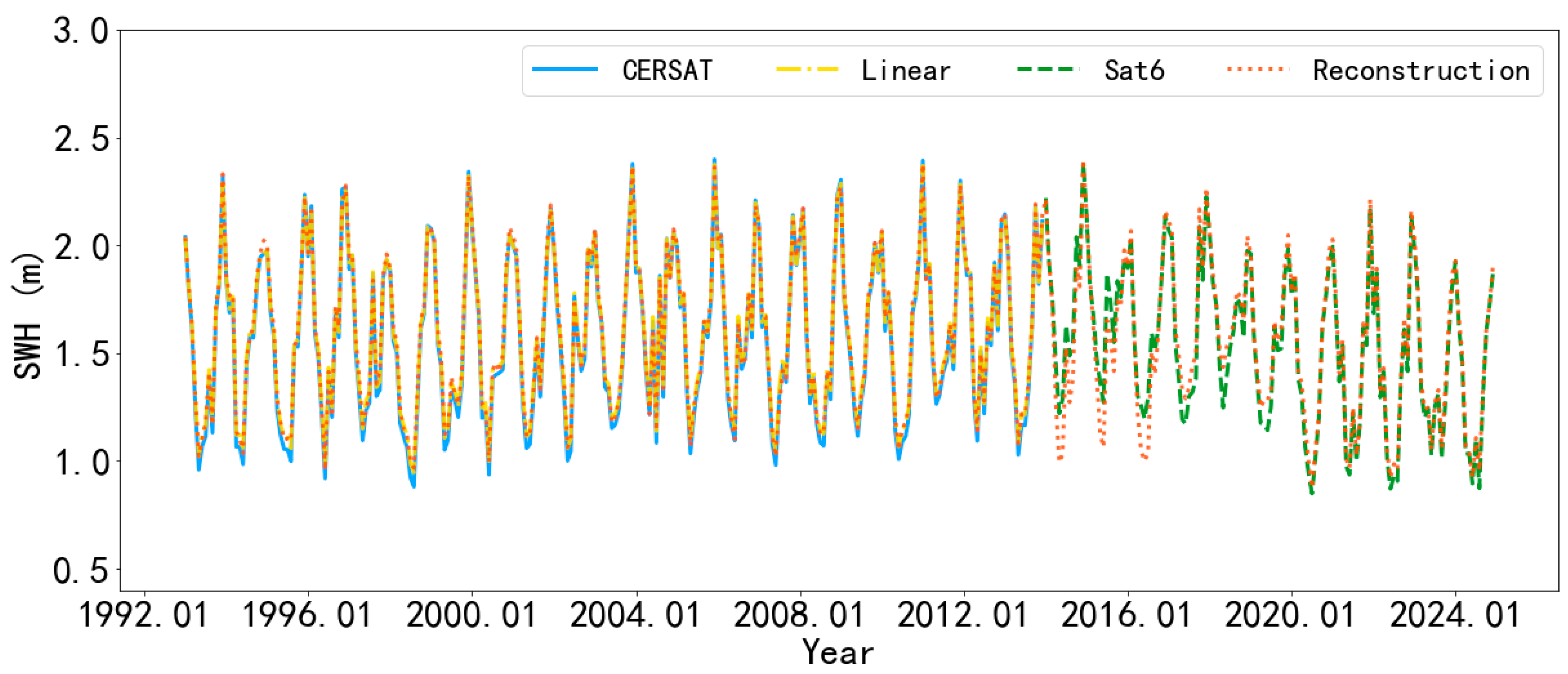
To reduce the systematic bias between the two altimeter swath-derived SWH datasets, data at grids with a distance of <50 km [16,17] in the two datasets on the same day during 2015–2016 were used as matched SWHs in the linear regression. For this linear regression, the Sat6 data, which have been calibrated using buoy observations from China’s offshore waters [16], were taken as reference data to validate CERSAT SWHs (Figure 2).

2.2. Method

The key to reconstruction of missing values is to capture spatial features from the background, e.g., ERA5 SWHs (the fifth generation ECMWF reanalysis). In recent years, advances in deep learning methods have improved the extraction of spatial features from reanalysis datasets. To fulfill this work in this study, we applied a partial convolutional U-Net model with attention and residual blocks. To solve for missing values over land, the partial convolutional U-Net was applied. According to the literature, the partial convolutional U-Net can effectively eliminate the influence from land [30]. The attention block was used to enhance the learning accuracy of identifying SWH using limited altimeter swaths data. The residual block was selected to enhance the learning efficiency of the model and enable faster convergence of the loss function.

2.2.1. Residual Attention CNN

A CNN is developed based on deep neural networks and various types of hidden layers, such as convolutional layers, pooling layers, activation layers, and fully connected layers [31]. Unlike traditional deep neural networks, a CNN utilizes convolutional kernels to perform convolution operations, enabling it to effectively understand the spatial hierarchical relationship and capture detailed features from two-dimensional variables [32].
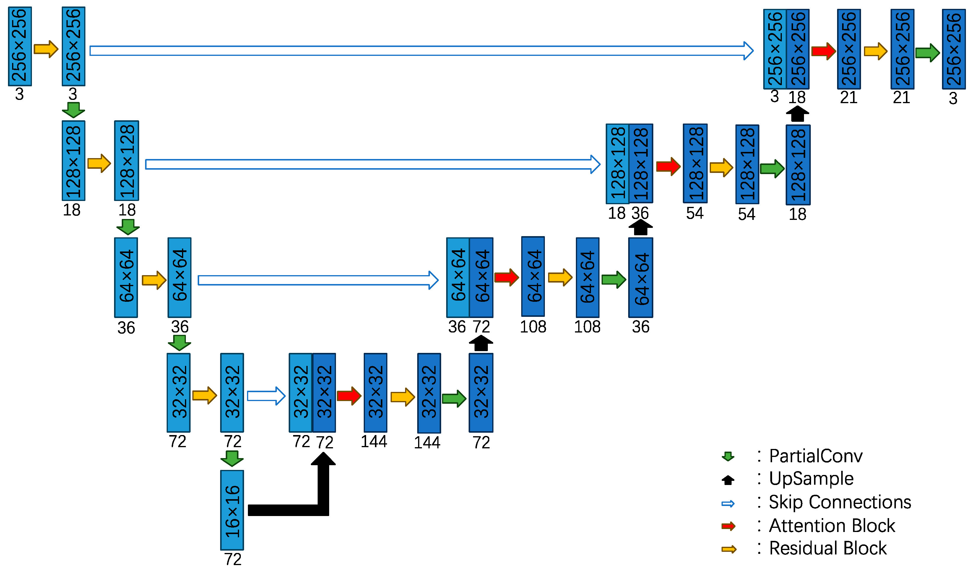
U-Net is a special type of CNN that is applied widely to image inpainting tasks [33]. Moreover, to more effectively capture the detailed gradient features of SWHs from high-resolution satellite observations, we incorporated partial convolutional, residual, and attention blocks into U-Net (Figure 3) to help alleviate the vanishing gradient problem and strengthen U-Net’s emphasis on key features [34]. To accelerate the convergence of the U-Net model loss function and improve training efficiency, three channels were used, as described in the literature [30,35].
Based on the partial convolutional layer principles in image inpainting [36], and similarly to other research enhancing the effectiveness of the U-Net model in extracting spatial characteristics [35], we replaced the standard convolutional layers with partial convolution layers in the U-Net structure. Unlike the direct computation of traditional convolution kernels, the partial convolution layer divides the convolution operation into two parts: the partial convolution and the updated mask. The calculation formula is as follows:
  X = W T X M s u m 1 s u m M + b ,                             i f   s u m M > 0 0 ,                                                                                                   o t h e r w i s e ,
where WT denotes the convolutional kernel, X denotes the input values, and M is the corresponding mask. The term 1/sum(M) denotes the impact of the number of valid values within the convolutional region, and ⊙ denotes the Hadamard product, i.e., the element-wise multiplication of matrices. The partial convolution operates only on regions within the convolutional area that contain at least one valid value of 1. Moreover, the convolution results vary depending on the number of real values within the convolutional region.
The updated mask refers to modification of those regions within the convolutional area that contain at least one valid value. Regions with valid values are updated to 1, while regions without valid values are updated to 0. The calculation formula is as follows:
M =   1 ,                 i f   s u m ( M ) > 0     0 ,                 o t h e r w i s e                     ,  
Based on ablation experiments, to further enhance the accuracy of the reconstructed results from the observed data, residual and attention blocks were incorporated into the model (Table 1). The residual network is divided into a direct mapping part and a residual part. After each convolution operation, the resulting value is added to the value prior to the convolution operation and this summed value is used as the input for the next neuron. The calculation formula is as follows:
x l + 1 = W l x l + F ( x l , W l ) ,            
where x l + 1 denotes the input to the next neuron, x l denotes the input to the current neuron, and W l ′ is a 1 × 1 convolution operation, which is applied to adjust the format of x l , ensuring that the number of channels of x l matches that of x l + 1 . Equations (6)–(8) are from the literature [30,35], and the adjustment allows for proper addition in the residual connection and consistency in the number of channels in the input and output. Here, F x l , W l denotes the value obtained after convolving x l . The residual block further strengthens the ability of the model to transfer information. Additionally, during the decoding phase in the reconstructed area, the data undergo attention-based weighting, which enhances the learning of attention weights from the real values. Overall, the above operations increase the influence of valid data on the reconstruction results, ultimately improving the accuracy of the reconstruction results.

2.2.2. SWH Reconstruction Process

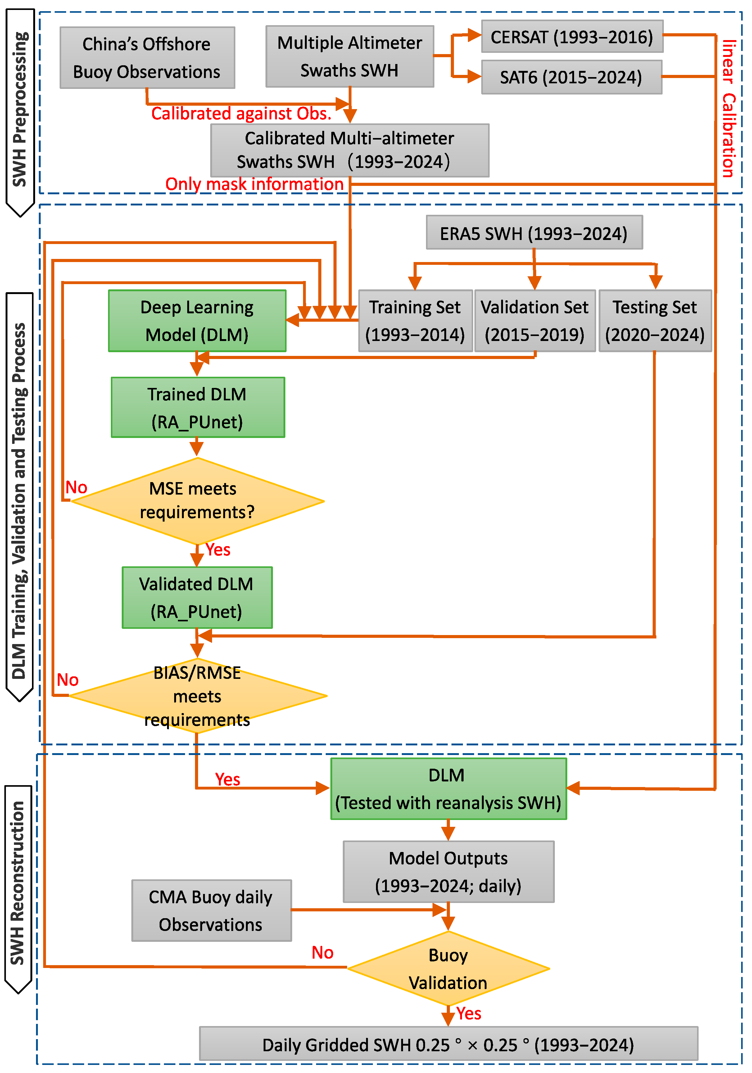
The objective of this study was to fill missing SWH values between altimeter swaths during 1993–2024. The ERA5 SWHs were selected as the background, while the altimeter SWH positions were used as mask data. To avoid leakage between training and test periods, data from 1993 to 2014, 2015 to 2019, and 2020 to 2024 were used as the training set, validation set, and test set, respectively. For the training set, the mask of one day in 1993–2024 from the altimeters was randomly assigned with ERA5 in 1993–2014 to enhance the ability of the model to determine the spatial structure. The efficacy of this random masking strategy has been validated in multiple machine learning and deep learning studies [37]. The specific process adopted was as follows. First, to complete the convolution process on land in the training set, the K-nearest neighbor interpolation method is used to interpolate SWH from sea to land. Then, corresponding spatiotemporal fields are selected for the region 10–44°N, 105–160°E, for which there are 256 grid points latitudinally and 256 grid points longitudinally. The dataset is preprocessed using mean–variance normalization, which is also called standardization, using multiyear monthly averages and STDs. Finally, the normalized training and validation sets, together with their corresponding mask values, are input into the model for training (Figure 4).
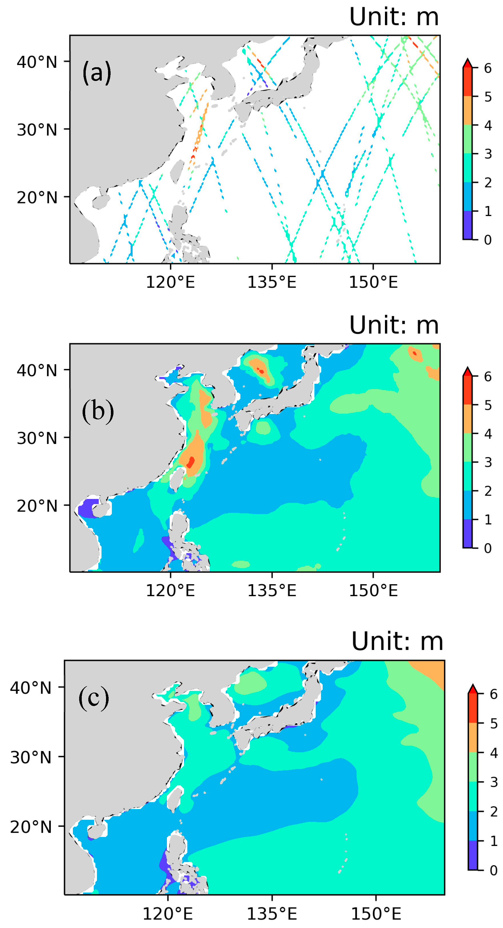
An Adam-based optimizer was employed with an initial learning rate of 2 × 10⁻⁴, a batch size of 30, and training conducted over 6000 iterations. Batch normalization was applied within the residual blocks, while the encoder’s batch normalization layer was frozen. The loss function comprised multiple weighted components (with a weight of 1 for the true region and 6 for the missing region), and the total loss was the weighted sum of these components. During training, both training and validation set losses are monitored simultaneously. Models are saved every 500 iterations, with visual evaluations conducted every 500 iterations. The reconstructed images are checked to ensure that the reconstructed SWHs are being processed correctly, and the reconstruction results are compared with the original swath-derived SWHs to evaluate the influence of these processes on the original swath data. Model parameters are adjusted continually until the loss function in the training set no longer decreases, or until the loss function decreases in the training set but increases in the validation set, at which point the model parameters are considered determined. As an example, Figure 5 shows the results for 23 January 2023, illustrating the coverage of the original swath-derived SWHs, the reconstructed SWHs, and the ERA5 SWHs. It is evident that the spatial features of the ERA5 and reconstructed SWHs are similar, and that in the original swath position, the swath-derived SWH values control the values of the reconstructed SWHs (Figure 5).

3. Results

3.1. Validation of the Reconstructed SWHs and Their Comparison with ERA5 SWHs

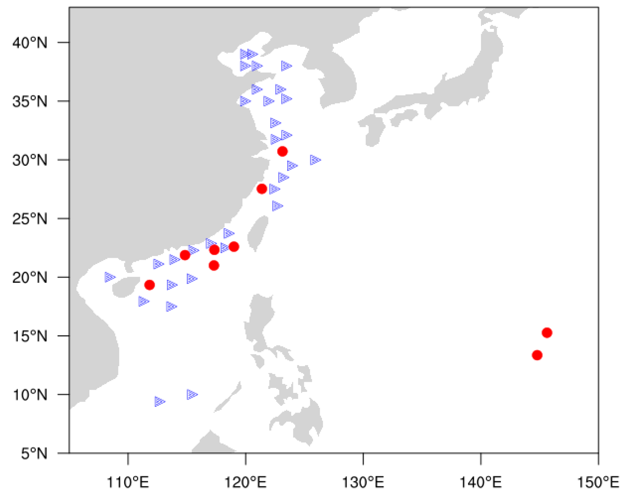
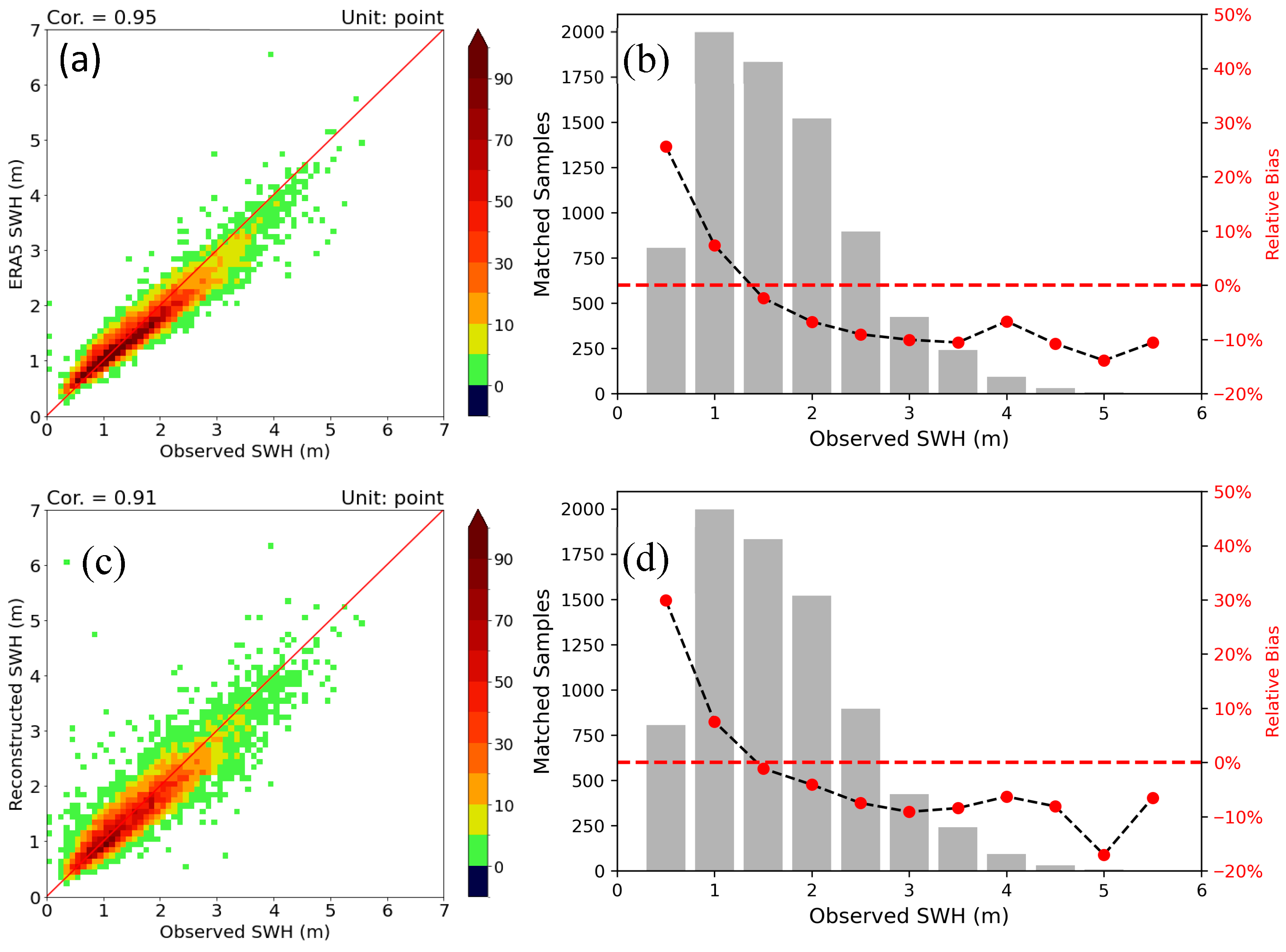
To obtain a general awareness of the quality of the reconstructed SWHs, daily SWHs from the reconstruction and buoy observations were compared. The buoy data were not used in the calibration of the altimeter-derived SWHs (Figure 6). The reconstructed SWHs are broadly consistent with the observed SWHs, and the variance of the reconstructed SWHs also agrees well with the observations with a temporal correlation coefficient of 0.91 (Figure 7a). Generally, the accuracy of the reconstructed SWHs is similar to that of the ERA5 SWHs, with RMSE and SI values for the ERA5 (reconstructed) SWHs of 0.26 m (0.31 m) and 0.15 (0.19), respectively. The relative bias in each 0.5 m interval of the observations indicates that the magnitude of the reconstructed SWHs is slightly less than that of the observations, with a relative bias of approximately −10% in the SWH range of 1.25–4.25 m (Figure 7b). It is worth noting that the original swath SWHs are greater than the in situ SWHs, even though we calibrated the SWH of each altimeter before using them in the reconstruction process [16], Therefore, the negative bias is derived mainly from the ERA5 data during the reconstruction processes, the values of which are usually less than the observations for SWHs of >1.5 m [38] (Figure 7c,d). The quality of the reconstructed daily SWHs is as good as that of the 10-day mean results, for which the relative bias is between approximately −10% and 15% [16]. These results indicate that application of the deep learning method in combination with the ERA5 SWHs improves the temporal resolution of the derived SWHs from 10 days to the daily scale. Moreover, the relative bias of the reconstructed SWHs is less compared with that of the ERA5 SWHs for heights of >1.5 m but greater in the range of approximately 0.5–1 m, meaning that the reconstructed SWHs have an advantage for greater SWHs.
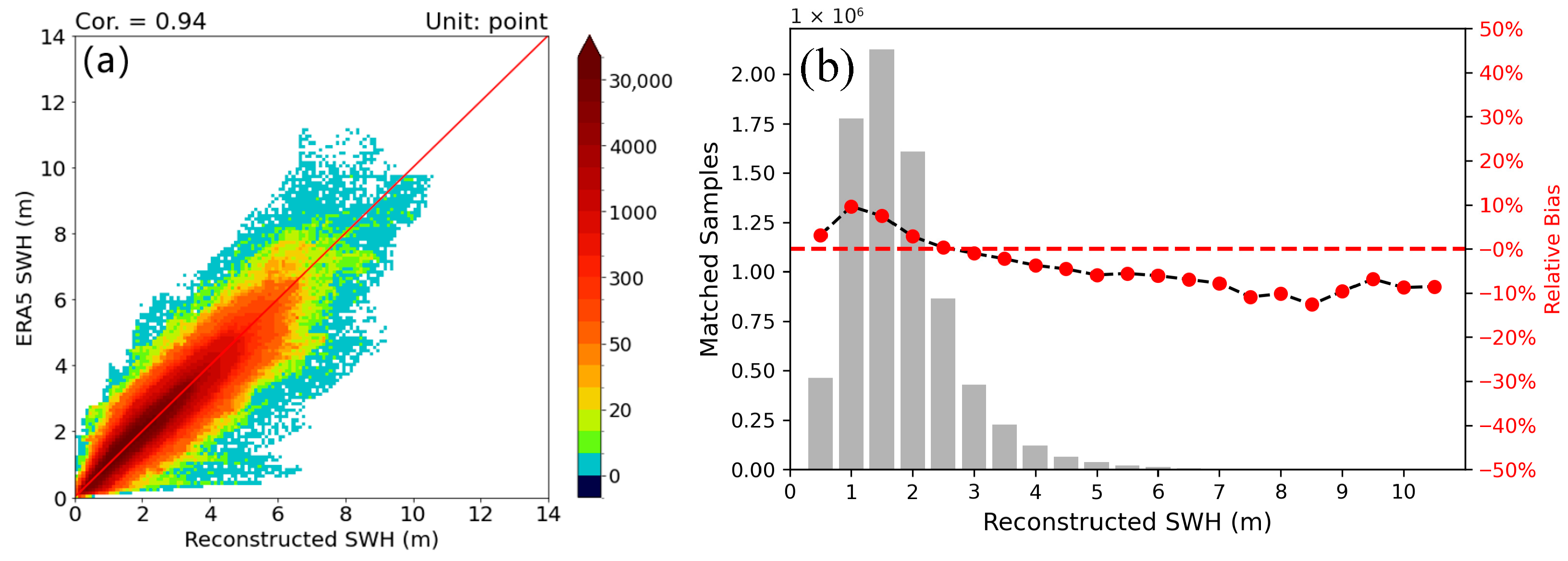
Furthermore, to analyze the differences between the U-Net background ERA5 SWHs and the reconstruction results, we also compared the daily reconstructed SWHs with the ERA5 SWHs in 2023 and the ERA5 SWHs with all buoy observations. The differences in SWH between the ERA5 and reconstructed data indicate that the reconstructed SWHs agree well with the ERA5 SWHs (Figure 8a). However, comparison with the buoy observations reveals that for SWHs over >2.5 m, the reconstructed SWHs have a greater value than the corresponding ERA5 SWHs (Figure 8b), meaning that the reconstructed SWHs have improved accuracy relative to the ERA5 SWHs, which are usually underestimated for SWHs of >2.5 m.
The retrieval algorithm for SWHs relies on the principle that at near-nadir incidence, the normalized radar cross-section is sensitive to the local slope of sea waves [39]. In calm sea conditions, the signal-to-noise ratio is relatively low, meaning that the accuracy of altimeter SWHs is lower for SWHs of <1 m than for SWHs of >2.5 m.

3.2. Differences in Spatial Distribution Between ERA5 SWHs and Reconstructed SWHs

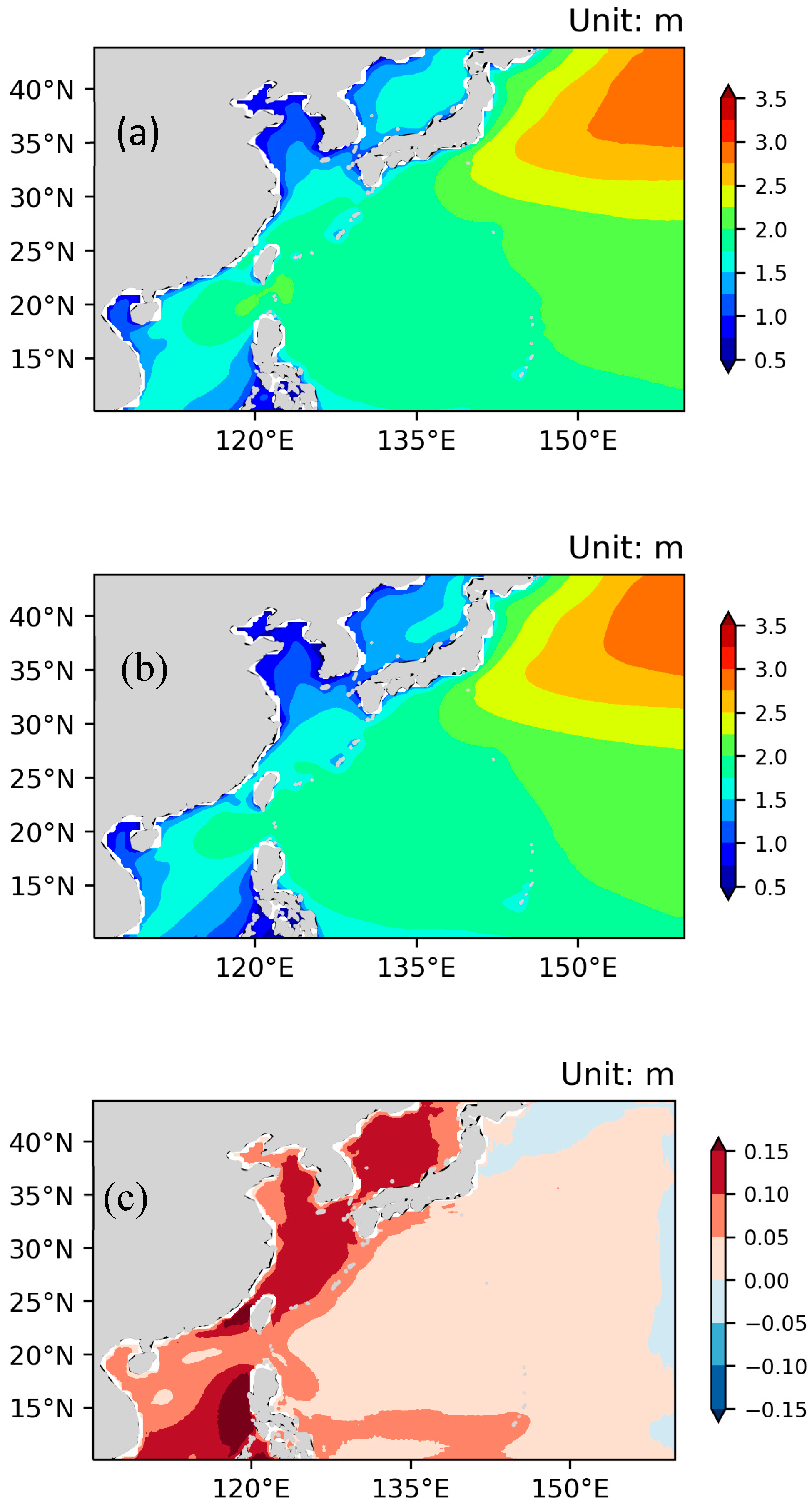
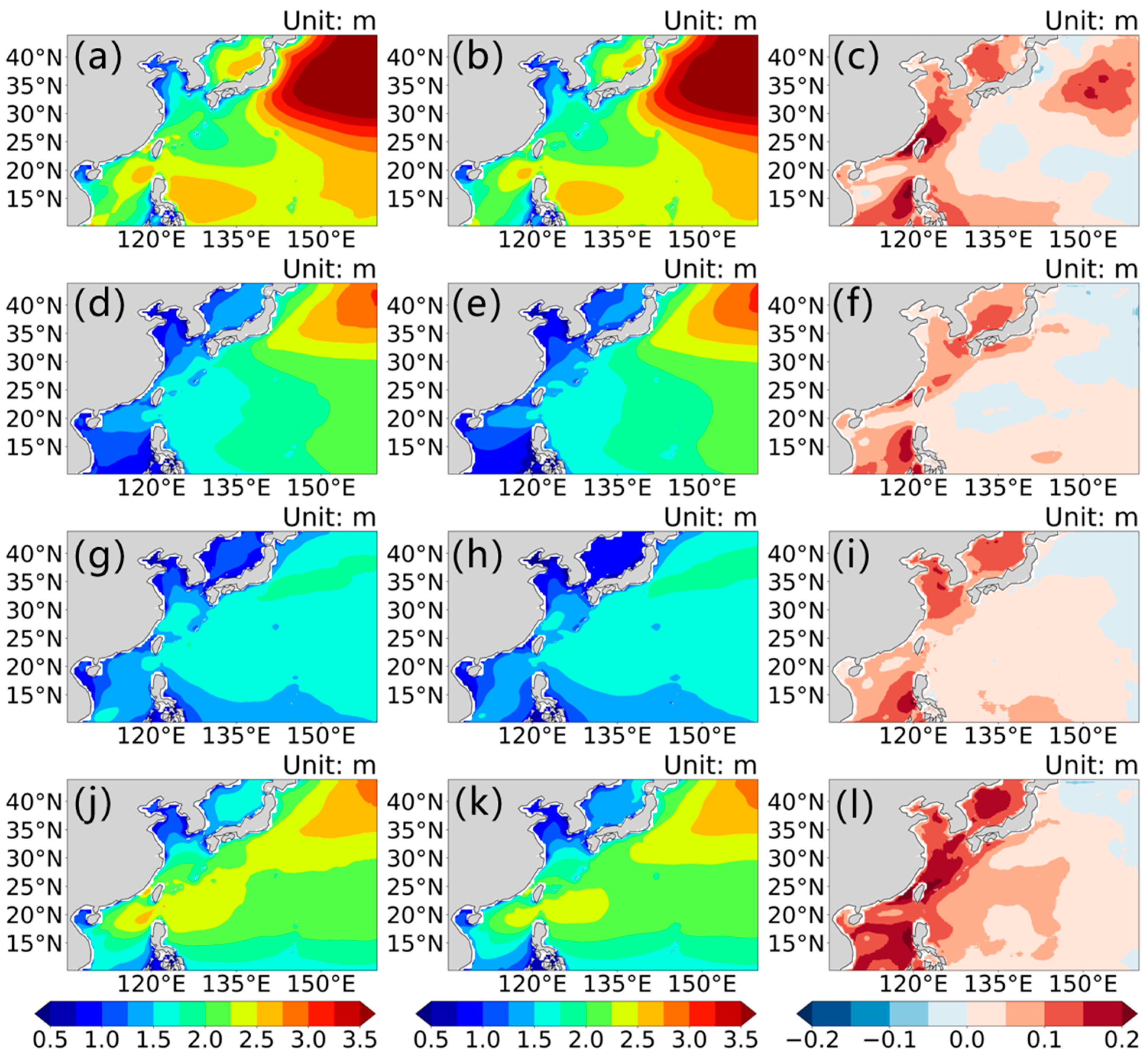
Generally, the features of SWH distribution are similar between the reconstructed data and the ERA5 data, with the highest SWH values in waters in the region of the East Asia Deep Trough (EADT) and lower values in northern parts of China’s offshore waters (Figure 9a,b). However, in almost all areas, the multiyear mean SWHs are higher in the reconstructed data than in the ERA5 data, especially in China’s offshore waters, where the reconstructed SWHs are greater than the ERA5 SWHs by around 0.1 m. The greatest differences are evident in the region of straits and waters influenced by robust air–sea interactions, e.g., the Taiwan Strait, Tsushima Strait, Bashi Channel, and the area affected by the Huanghai Warm Current (Figure 9c).
To analyze the differences in the seasonal spatial distribution between the ERA5 SWHs and the reconstructed SWHs, the monthly mean differences in representative months during 1993–2024 are compared in Figure 10. In winter, represented by January, the main distribution of SWH is similar between the reconstruction and ERA5, with both exhibiting higher SWHs in waters in the region of the EADT and lower SWHs in China’s offshore waters (Figure 10a,b). However, in waters in the region of the EADT and in straits such as the Taiwan Strait and Bashi Channel, the reconstructed SWHs are visibly greater than the ERA5 SWHs (Figure 10c).
In spring and summer, represented by April and July, respectively, the general distributions are the same between the reconstructed SWHs and the ERA5 SWHs (Figure 10d,e,g,h), where the greatest differences in the studied waters are found near the Taiwan Strait and in the Bashi Channel (Figure 10f,i).
In autumn, represented by October, when northerly winds are dominant, the greatest seasonal differences in SWH are evident. The main distribution of the reconstructed SWHs is similar to that of the ERA5 SWHs, with the highest SWHs in the region of the EADT and lower SWHs in northern parts of China’s offshore waters (Figure 10j,k). The greatest differences in SWH within the study area are in the region influenced by the Huanghai Warm Current and in straits such as the Taiwan Strait (Figure 10l).
Generally, the pattern of SWHs is similar between the reconstructed data and the ERA5 data; however, the main differences are the greater SWHs in areas such as the Taiwan Strait and in regions of robust air–sea interaction such as the regions influenced by the Huanghai Warm Current and the Kuroshio Current. This result indicates that in complex straits and under high sea state conditions, the wind-driven wave heights in the ERA5 data are not as high as those obtained directly from altimeter observations.

3.3. Differences in Linear Trends Between ERA5 SWHs and Reconstructed SWHs

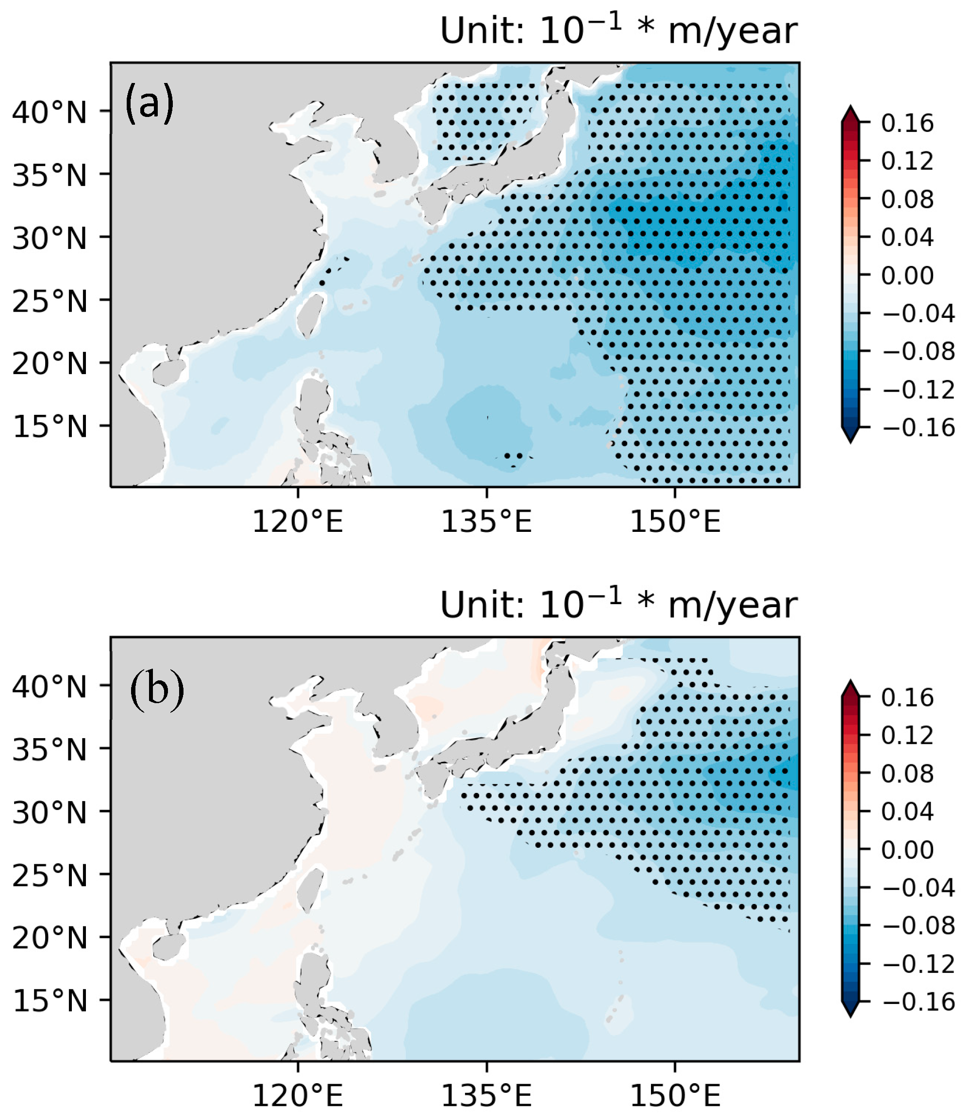
The linear trend of SWH is an important element that reveals the variance in the strength of air–sea interaction over the long term, e.g., 1993–2024. To eliminate the influence of seasonal cycles, we calculated the yearly mean SWH value and then computed its linear trend. The results reveal a uniformly negative trend across the entire research area for the reconstructed SWHs (Figure 11a), whereas the ERA5 SWHs show a pattern with a slight positive trend in the offshore waters of China and the Philippines and a negative trend in most open-ocean waters to the east of approximately 130°E, but with the greatest statistically significant trend to the east of 150°E and between 25°N and 40°N (Figure 11b). It is worth noting that the magnitude of the trend of the reconstructed SWHs is greater than that of the ERA5 data, which indicates that the negative trend of the SWHs from remote sensing is greater than that from numerical simulation. Moreover, in China’s offshore waters, a statistically significant negative linear trend in the reconstructed SWHs is evident only in the region to the north of the Taiwan Strait.
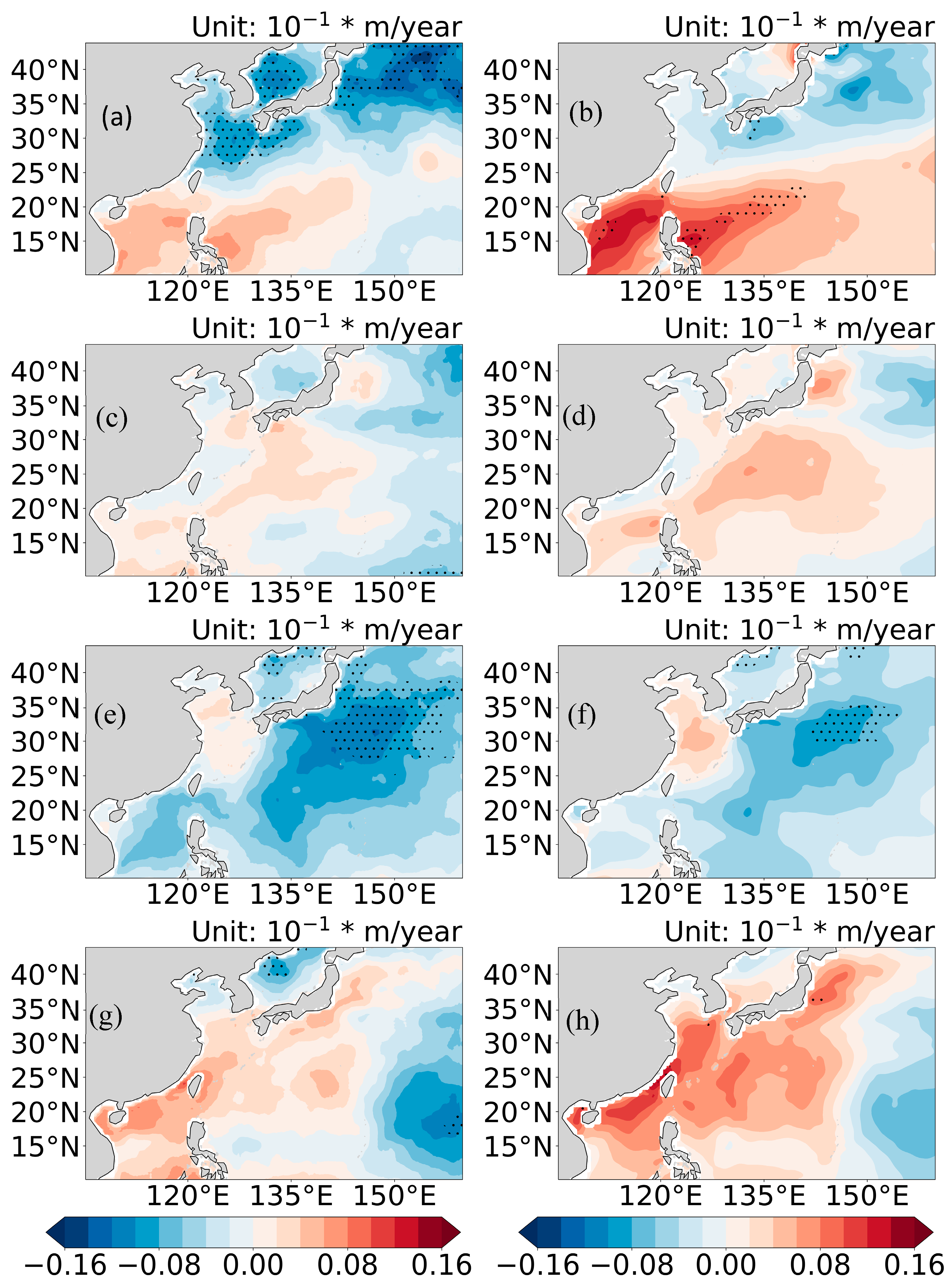
Given the dramatic changes in the dominant wind on the seasonal scale, the linear trends of the variance in SWH from the reconstruction and from ERA5 for each month representative of a season were analyzed. The patterns of the trend in SWH from the reconstruction and ERA5 agree well with each other (Figure 12), although the negative trends among the four representative months are greater for the reconstructed SWHs than for the ERA5 SWHs.
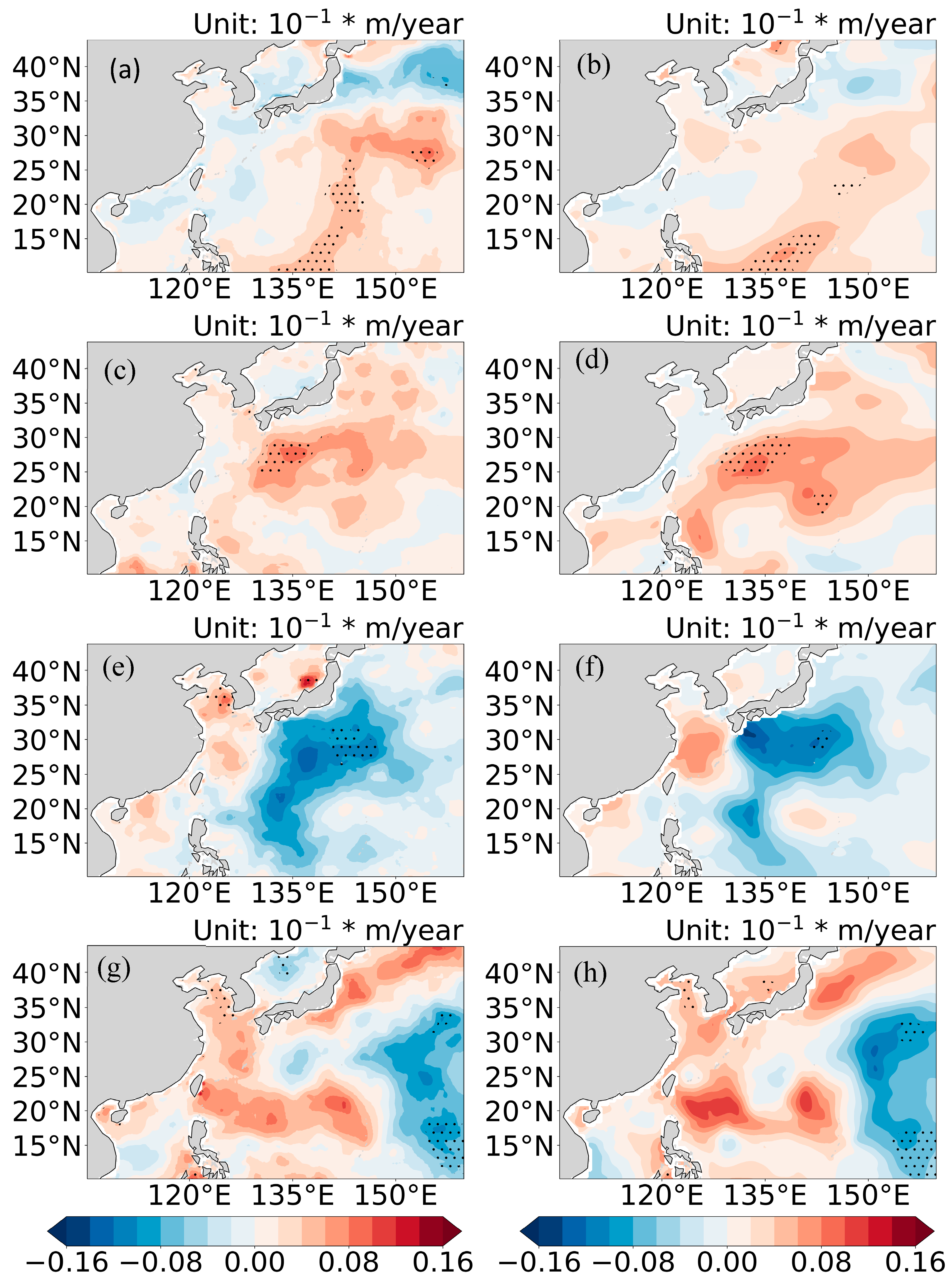
In winter, represented by January, the linear trends of SWH for both datasets show similar distributions and greater negative trends over the northwestern Pacific Ocean (Figure 12a,b). The magnitude of the positive linear trend of ERA5 SWHs is greater than that of the reconstructed SWHs in the region of the South China Sea and to the east of the Philippines in January. In April, the month taken as representative of spring, the magnitude of the linear trend is weaker in comparison with that in other seasons and no waters exhibit a statistically significant trend (Figure 12c,d). In July, boreal summer, the magnitude of the negative linear trend is greater for the reconstructed SWHs than for the ERA5 SWHs around 150°E (Figure 12e,f). In October, representative of autumn, the linear trends of both datasets show no obvious signal in terms of SWH variance (Figure 12g,h).
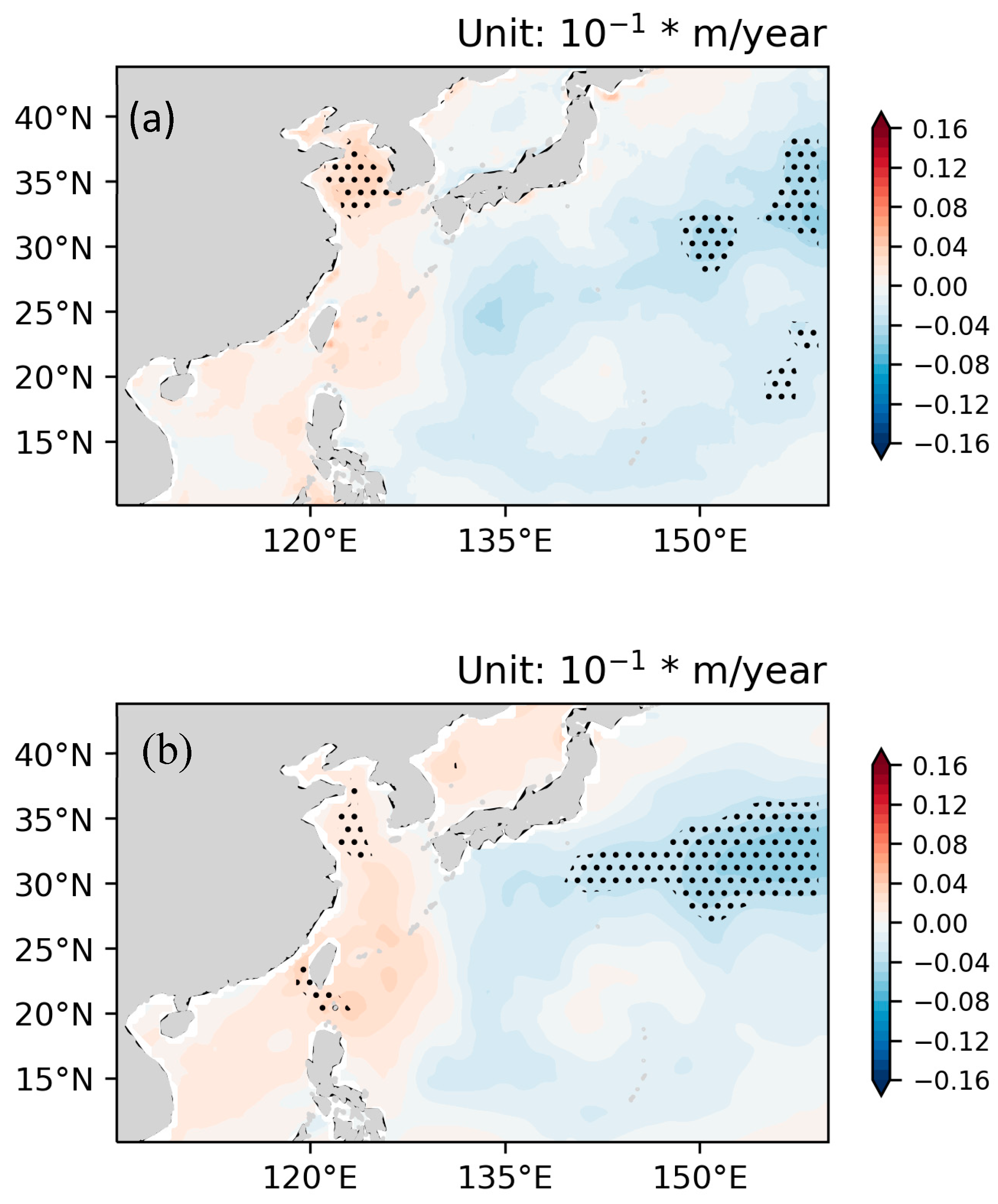
Additionally, the trend of the STDs indicates the magnitude of the variance of abnormal SWHs, which is also an important indicator of the variance of extreme SWH events, where a positive (negative) signal means an increase (decline) in extreme SWH events. The pattern of the reconstructed results is similar to that of the ERA5 results throughout the study area (Figure 13). It is worth noting that the magnitude of the positive trend in STDs is greater for the reconstructed data than for the ERA5 data over northern parts of China’s offshore waters, which means that the occurrence of extreme SWH events observed by altimeters is increasing relative to that derived from ERA5. However, the negative trend of the STDs of both datasets indicates that the variance in SWH is diminishing in waters to the east of 150°E.
The patterns of the trends of STDs in the four months representative of the seasons are similar for both datasets (Figure 14). However, for waters affected by the Huanghai Warm Current in October, the positive trend of the STD signal is greater for the reconstructed data than for the ERA5 data, indicating that abnormal variance increased visibly during 1993–2024.
Generally, to the east of 150°E, negative linear trends in SWHs and negative trends of STDs are both evident, indicating a stable decline in SWHs in that area. Furthermore, the magnitude of the trend of decline is greater for the reconstructed SWHs than for the ERA5 SWHs. The positive trend in the STDs in northern parts of China’s offshore waters indicates that the magnitude of abnormal SWHs increased during the study period. Similarly to the greater negative signal for the reconstructed data in the region to the east of 150°E, this signal is also greater for the reconstructed SWHs than for the ERA5 SWHs.

4. Discussion

This work focused on developing a deep learning method to fill gaps in long-term daily high-resolution gridded SWHs, comparing the quality of reconstructed SWHs against in situ observations and revealing the long-term linear trend characteristics of reconstructed SWHs. The major differences between the reconstructed SWHs and the ERA5 SWHs were found in the region of straits and in waters influenced by robust air–sea interactions. Therefore, it is important to note that robust air–sea interactions can lead to uncertainty in SWH values, especially when the weather system process generates high sea conditions. Despite the relatively limited number of observations, comparisons with data from 38 buoys moored in China’s offshore waters revealed broadly consistent results between the reconstructed SWHs and the ERA5 SWHs. This finding emphasizes the need for special attention regarding the method used for effective extraction of the spatial features of SWH. Advances in other approaches, such as using a generative model, exploiting the advantages of numerical simulations of SWHs, and obtaining altimeter-derived gridded SWH data with higher temporal resolution (e.g., 6 h), represent promising areas for further development of the proposed method.

5. Conclusions

High-resolution spatial gridded altimeter-derived SWH data with daily temporal resolution can reveal details of the influencing processes of weather systems on the ocean. Moreover, long-term gridded altimeter-derived SWH data can reveal the variance in the strength of air–sea interactions under the background of climate change. However, owing to the sparse coverage and narrow swath width of satellite-borne altimeters, the main obstacle is compensating for the numerous missing SWH values around the daily swaths. Even before the development of deep learning methods, it was possible to effectively extract the spatial features of ERA5 SWHs, which substantially enhanced the feasibility of filling missing values. However, in this study, we used a partial convolutional U-Net model with attention and residual blocks, adopting ERA5 SWHs as a background and altimeter swath-derived SWHs as the constraint condition, to reconstruct gridded altimeter-derived SWHs during 1993–2024. We then analyzed the quality of the reconstructed SWHs against in situ observations of SWH and compared them with the ERA5 SWHs. The results showed that the reconstructed SWHs agreed well with the in situ observations and that the bias was as good as that of 10-day mean SWHs. The reconstructed SWHs improved the accuracy for SWHs of >2.5 m, which are usually underestimated in the ERA5 data. In regions with high SWHs, the reconstructed values were generally greater than those of ERA5. The magnitude of the negative linear trend of SWHs from the reconstruction was greater than that from ERA5 around 150°E. Although this study developed a method to fill missing SWHs around altimeter swaths, further systematic studies will be necessary to investigate other deep learning methods for more effective and precise extraction of the spatial distribution features of SWHs. The main results of this study are summarized in the following points.
(1)
The proposed partial convolutional U-Net model with attention and residual blocks can effectively extract the spatial features of ERA5 SWHs and fill missing values around the daily altimeter swaths. Consideration of the results for a single day, as an example, revealed that the spatial features of the ERA5 and reconstructed SWHs are similar. Furthermore, in the original swath position, the SWH values can control the values in the reconstruction results in the same position.
(2)
The reconstructed daily SWHs are lower than the observations, with relative bias of approximately −10% for SWHs between 1.25 and 4.25 m, the quality of which is as good as that of 10-day mean SWHs, but with dramatic improvement in temporal resolution. The reconstructed SWHs improve accuracy for SWHs of >2.5 m, which are usually underestimated in the ERA5 data.
(3)
Although the spatial distribution of the reconstructed SWHs is similar to that of the ERA5 SWHs, the greatest differences are found in China’s offshore waters, especially in straits and waters influenced by robust air–sea interactions, e.g., the Taiwan Strait and the region affected by the Huanghai Warm Current. This indicates that ERA5 underestimates both the intensity of wind in straits and the strength of air–sea interactions.
(4)
For the period 1993–2024, the negative trend of SWHs from the reconstruction is greater than that of SWHs from ERA5, especially in waters to the east of 150°E. Moreover, the reconstructed SWHs revealed an obvious positive trend in STDs over northern parts of China’s offshore waters, indicating that the magnitude of abnormal SWHs has increased during the study period.

Author Contributions

J.X. initiated and coordinated the work. Y.Z. and L.Y. provided the calculation and validation. J.X. and Y.Z. wrote the manuscript. Z.M. and Y.L. supplied software on the U-Net model. X.Z. (Xiefei Zhi), X.Z. (Xiuzhi Zhang), Y.X. and L.K. gave valuable suggestions for revisions. X.Z. (Xiefei Zhi) revised the analysis. All authors have read and agreed to the published version of the manuscript.

Funding

This research was jointly supported by the project entitled “Research on 8-42d Subseasonal Multi-mode Integrated Forecasting Based on Statistical Methods and Machine Learning” supported by the National Natural Science Foundation of China (grant numbers 42275164), the Civil Aviation Safety Operation Support Capability Construction Project, GrantsKG2025005, project 2023CFO018 supported by the Key Laboratory of Space Ocean Remote Sensing and Application, MNR and National Natural Science Foundation of China (grant numbers 41005057). Also, we acknowledge the High Performance Computing Center of Nanjing University of Information Science & Technology for their support of this work.

Data Availability Statement

Data are available upon request.

Acknowledgments

We thank anonymous reviewers for comments and suggestions that helped to improve the manuscript. Also, we thank CNSA and CNES for providing the CFOSAT data, NSOAS for providing the HY–2A, HY–2B, and HY–2C data, global altimeter SWH Ifremer database for providing Jason–2 and Cryosat–2 data, and SOAC and CMA for providing the buoy observations. The ECMWF ERA5 hourly data on levels can be accessed from the Copernicus Climate Change Service Climate Data Store [40], https://cds.climate.copernicus.eu/#!/home (accessed on 20 November 2025). We also thank the National Buoy Data Center for providing the buoy observations used in this paper. The code for the partial convolutional U-Net model with attention and residual blocks is available at https://doi.org/10.5281/zenodo.17641790 (accessed on 20 November 2025).

Conflicts of Interest

The authors declare no conflicts of interest.

References

  1. Han, X.; Wang, X.; He, Z.; Wu, J. Significant Wave Height Retrieval in Tropical Cyclone Conditions Using CYGNSS Data. Remote Sens. 2024, 16, 4782. [Google Scholar] [CrossRef]
  2. Xu, J.; Zhi, X.; Sein, D.V.; Cabos, W.; Luo, Y.; Zhang, L.; Dong, F.; Fraedrich, K.; Jacob, D. Predictability of Coastal Boundary Layer Jets in South China Using Atmosphere–Ocean Coupling. J. Geophys. Res. Atmos. 2023, 128, e2023JD039184. [Google Scholar] [CrossRef]
  3. Zhang, S.; Zhou, R.; Jia, Y.; Jin, T.; Kong, X. Performance of HaiYang-2 Altimetric Data in Marine Gravity Research and a New Global Marine Gravity Model NSOAS22. Remote Sens. 2022, 14, 4322. [Google Scholar] [CrossRef]
  4. Aboobacker, V.M.; Shanas, P.R.; Al-Ansari, E.M.A.S.; Sanil Kumar, V.; Vethamony, P. The maxima in northerly wind speeds and wave heights over the Arabian Sea, the Arabian/Persian Gulf and the Red Sea derived from 40 years of ERA5 data. Clim. Dyn. 2021, 56, 1037–1052. [Google Scholar] [CrossRef]
  5. Wang, J.; Yu, T.; Deng, F.; Ruan, Z.; Jia, Y. Acquisition of the Wide Swath Significant Wave Height from HY-2C through Deep Learning. Remote Sens. 2021, 13, 4425. [Google Scholar] [CrossRef]
  6. Bué, I.; Lemos, G.; Semedo, Á.; Catalão, J. Assessment of satellite altimetry SWH measurements by in situ observations within 25 km from the coast. Ocean Dyn. 2024, 74, 183–210. [Google Scholar] [CrossRef]
  7. Grigorieva, V.G.; Badulin, S.I.; Gulev, S.K. Global Validation of SWIM/CFOSAT Wind Waves Against Voluntary Observing Ship Data. Earth Space Sci. 2022, 9, e2021EA002008. [Google Scholar] [CrossRef]
  8. Kang, J.; Mao, R.; Chang, Y.; Fu, H. Comparative analysis of significant wave height between a new Southern Ocean buoy and satellite altimeter. Atmos. Ocean. Sci. Lett. 2021, 14, 100044. [Google Scholar] [CrossRef]
  9. Müller, M.; Knol-Kauffman, M.; Jeuring, J.; Palerme, C. Arctic shipping trends during hazardous weather and sea-ice conditions and the Polar Code’s effectiveness. NPJ Ocean Sustain. 2023, 2, 12. [Google Scholar] [CrossRef]
  10. Woo, H.-J.; Park, K.-A. Estimation of Extreme Significant Wave Height in the Northwest Pacific Using Satellite Altimeter Data Focused on Typhoons (1992–2016). Remote Sens. 2021, 13, 1063. [Google Scholar] [CrossRef]
  11. Quartly, G.D.; Chen, G.; Nencioli, F.; Morrow, R.; Picot, N. An Overview of Requirements, Procedures and Current Advances in the Calibration/Validation of Radar Altimeters. Remote Sens. 2021, 13, 125. [Google Scholar] [CrossRef]
  12. Ribal, A.; Young, I.R. 33 years of globally calibrated wave height and wind speed data based on altimeter observations. Sci. Data 2019, 6, 77. [Google Scholar] [CrossRef]
  13. Young, I.R.; Ribal, A. Multiplatform evaluation of global trends in wind speed and wave height. Science 2019, 364, 548–552. [Google Scholar] [CrossRef]
  14. Timmermans, B.W.; Gommenginger, C.P.; Dodet, G.; Bidlot, J.R. Global Wave Height Trends and Variability from New Multimission Satellite Altimeter Products, Reanalyses, and Wave Buoys. Geophys. Res. Lett. 2020, 47, e2019GL086880. [Google Scholar] [CrossRef]
  15. Dodet, G.; Piolle, J.F.; Quilfen, Y.; Abdalla, S.; Accensi, M.; Ardhuin, F.; Ash, E.; Bidlot, J.R.; Gommenginger, C.; Marechal, G.; et al. The Sea State CCI dataset v1: Towards a sea state climate data record based on satellite observations. Earth Syst. Sci. Data 2020, 12, 1929–1951. [Google Scholar] [CrossRef]
  16. Xu, J.; Wu, H.; Zhi, X.; Koldunov, N.V.; Zhang, X.; Xu, Y.; Zhang, Y.; Guo, M.; Kong, L.; Fraedrich, K. Validation of Multisource Altimeter SWH Measurements for Climate Data Analysis in China’s Offshore Waters. Remote Sens. 2024, 16, 2162. [Google Scholar] [CrossRef]
  17. Xu, J.; Wu, H.; Xu, Y.; Koldunov, N.V.; Zhang, X.; Kong, L.; Xu, M.; Fraedrich, K.; Zhi, X. Validation of Nadir SWH and Its Variance Characteristics from CFOSAT in China&rsquo;s Offshore Waters. Remote Sens. 2023, 15, 1005. [Google Scholar]
  18. Hersbach, H.; Bell, B.; Berrisford, P.; Hirahara, S.; Horányi, A.; Muñoz-Sabater, J.; Nicolas, J.; Peubey, C.; Radu, R.; Schepers, D.; et al. The ERA5 global reanalysis. Q. J. R. Meteorol. Soc. 2020, 146, 1999–2049. [Google Scholar] [CrossRef]
  19. Wang, J.; Wang, Y. Evaluation of the ERA5 Significant Wave Height against NDBC Buoy Data from 1979 to 2019. Mar. Geod. 2022, 45, 151–165. [Google Scholar] [CrossRef]
  20. Yang, Y.; Qi, J.; Yan, Q.; Fan, C.; Zhang, R.; Zhang, J. Reconstruction of Wide Swath Significant Wave Height From Quasi-Synchronous Observations of Multisource Satellite Sensors. Earth Space Sci. 2024, 11, e2023EA003162. [Google Scholar] [CrossRef]
  21. Qiao, X.; Zhang, K.; Huang, W. Impacts of Climate Change on Oceans and Ocean-Based Solutions: A Comprehensive Review from the Deep Learning Perspective. Remote Sens. 2025, 17, 2306. [Google Scholar] [CrossRef]
  22. Sardana, D.; Kumar, P.; Bhaskaran, P.K.; Nair, T.M.B. The projected changes in extreme wave height indices over the Indian Ocean using COWCLIP2.0 datasets. Clim. Dyn. 2023, 61, 255–269. [Google Scholar] [CrossRef]
  23. Queffeulou, P. Long-Term Validation of Wave Height Measurements from Altimeters. Mar. Geod. 2004, 27, 495–510. [Google Scholar] [CrossRef]
  24. Xu, Y.; Liu, J.; Xie, L.; Sun, C.; Liu, J.; Li, J.; Xian, D. China-France Oceanography Satellite (CFOSAT) simultaneously observes the typhoon-induced wind and wave fields. Acta Oceanol. Sin. 2019, 38, 158–161. [Google Scholar] [CrossRef]
  25. Haifeng, Z.; Qing, W.U.; Ge, C. Validation of HY-2A Remotely Sensed Wave Heights against Buoy Data and Jason-2 Altimeter Measurements. J. Atmos. Ocean. Technol. 2015, 32, 150402094232008. [Google Scholar]
  26. Jia, Y.; Yang, J.; Lin, M.; Zhang, Y.; Ma, C.; Fan, C. Global assessments of the HY-2B measurements and cross-calibrations with Jason-3. Remote Sens. 2020, 12, 2470. [Google Scholar] [CrossRef]
  27. Ye, X.; Lin, M.; Xu, Y. Validation of Chinese HY-2 satellite radar altimeter significant wave height. Acta Oceanol. Sin. 2015, 34, 60–67. [Google Scholar] [CrossRef]
  28. Donlon, C.; Berruti, B.; Buongiorno, A.; Ferreira, M.-H.; Féménias, P.; Frerick, J.; Goryl, P.; Klein, U.; Laur, H.; Mavrocordatos, C. The global monitoring for environment and security (GMES) sentinel-3 mission. Remote Sens. Environ. 2012, 120, 37–57. [Google Scholar] [CrossRef]
  29. Yang, J.; Zhang, J. Validation of Sentinel-3A/3B satellite altimetry wave heights with buoy and Jason-3 data. Sensors 2019, 19, 2914. [Google Scholar] [CrossRef]
  30. Ma, Z.; Huang, J.; Zhang, X.; Luo, Y.; Ding, M.; Wen, J.; Jin, W.; Qiao, C.; Yin, Y. Newly reconstructed Arctic surface air temperatures for 1979–2021 with deep learning method. Sci. Data 2023, 10, 140. [Google Scholar] [CrossRef] [PubMed]
  31. Chauhan, R.; Ghanshala, K.K.; Joshi, R.C. Convolutional Neural Network (CNN) for Image Detection and Recognition. In Proceedings of the 2018 First International Conference on Secure Cyber Computing and Communication (ICSCCC), Jalandhar, India, 15–17 December 2018; pp. 278–282. [Google Scholar]
  32. Liu, D.; Han, G.; Liu, P.; Yang, H.; Sun, X.; Li, Q.; Wu, J. A Novel 2D-3D CNN with Spectral-Spatial Multi-Scale Feature Fusion for Hyperspectral Image Classification. Remote Sens. 2021, 13, 4621. [Google Scholar] [CrossRef]
  33. Du, G.; Cao, X.; Liang, J.; Chen, X.; Zhan, Y. Medical image segmentation based on U-net: A review. J. Imaging Sci. Technol. 2020, 64, 1. [Google Scholar] [CrossRef]
  34. Zhang, Z.; Song, Q.; Duan, M.; Liu, H.; Huo, J.; Han, C. Deep Learning Model for Precipitation Nowcasting Based on Residual and Attention Mechanisms. Remote Sens. 2025, 17, 1123. [Google Scholar] [CrossRef]
  35. Ma, Z.; Huang, J.; Zhang, X.; Luo, Y.; Dou, T.; Ding, M. Deep learning-based reconstruction of monthly Antarctic surface air temperatures from 1979 to 2023. Sci. Data 2025, 12, 847. [Google Scholar] [CrossRef]
  36. Liu, G.; Dundar, A.; Shih, K.J.; Wang, T.-C.; Reda, F.A.; Sapra, K.; Yu, Z.; Yang, X.; Tao, A.; Catanzaro, B. Partial convolution for padding, inpainting, and image synthesis. IEEE Trans. Pattern Anal. Mach. Intell. 2022, 45, 6096–6110. [Google Scholar] [CrossRef] [PubMed]
  37. Bochow, N.; Poltronieri, A.; Rypdal, M.; Boers, N. Reconstructing historical climate fields with deep learning. Sci. Adv. 2025, 11, eadp0558. [Google Scholar] [CrossRef]
  38. Zhai, R.; Huang, C.; Yang, W.; Tang, L.; Zhang, W. Applicability evaluation of ERA5 wind and wave reanalysis data in the South China Sea. J. Oceanol. Limnol. 2023, 41, 495–517. [Google Scholar] [CrossRef]
  39. Hauser, D.; Tison, C.; Amiot, T.; Delaye, L.; Corcoral, N.; Castillan, P. SWIM: The First Spaceborne Wave Scatterometer. IEEE Trans. Geosci. Remote Sens. 2017, 55, 3000–3014. [Google Scholar] [CrossRef]
  40. Hersbach, H.; Bell, B.; Berrisford, P.; Biavati, G.; Horányi, A.; Muñoz Sabater, J.; Nicolas, J.; Peubey, C.; Radu, R.; Rozum, I.; et al. ERA5 hourly data on pressure levels from 1940 to present. Copernicus Climate Change Service (C3S) Climate Data Store (CDS). 2023. Available online: https://cds.climate.copernicus.eu/datasets/reanalysis-era5-pressure-levels?tab=overview (accessed on 20 November 2025). [CrossRef]
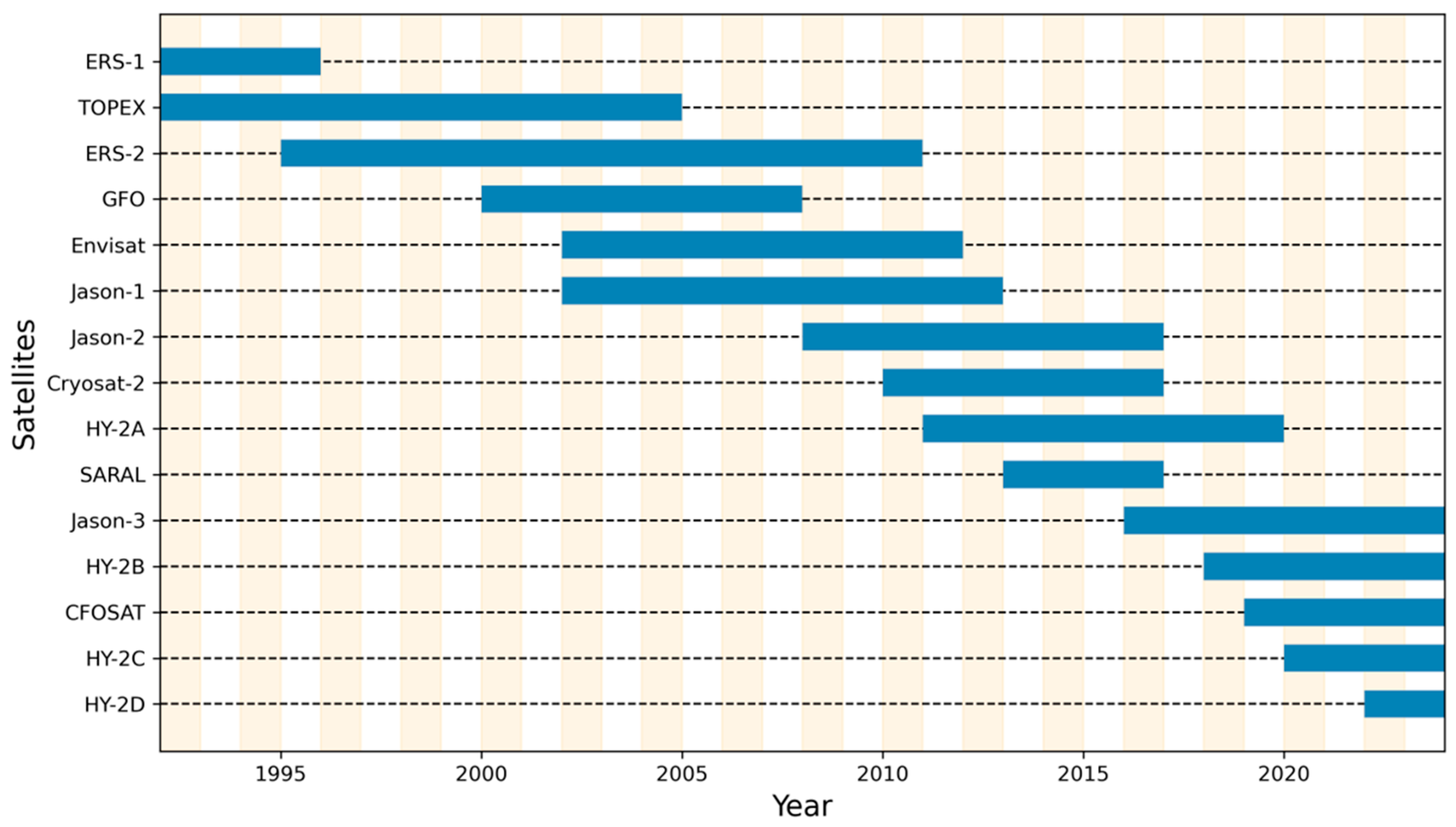
Figure 1. Span of altimeter observations, where HY-2A, HY-2B, HY-2C, HY-2D, CFOSAT, and Jason-3 represent the sources for the Sat6 SWH dataset.
Remotesensing 17 03802 g001
Figure 2. Variance in SWH in the search area based on the linear regression (yellow line), CERSAT from the GlobWave project (blue line), Sat6 (green line), and the reconstruction (red line).
Remotesensing 17 03802 g002
Figure 3. Schematic of the U-Net structure. Numbers inside the rectangular boxes indicate the dimensions of the image, and the value below each box indicates the number of channels. Green arrows represent partial convolution operations. Black arrows indicate upsampling operations via nearest neighbor interpolation. White arrows signify skip connections. Red arrows correspond to the attention block that adaptively emphasizes features in the input. Yellow arrows illustrate residual connections.
Remotesensing 17 03802 g003
Figure 4. Applied U-Net with the partial convolutional, residual, and attention workflow. “China’s Offshore Buoy Observations” are from the SOAC. “CMA Buoy daily Observations” are from the CMA.
Remotesensing 17 03802 g004
Figure 5. Example results for 23 January 2023, showing (a) altimeter swath-derived SWHs, (b) reconstructed SWHs, and (c) ERA5 SWHs.
Remotesensing 17 03802 g005
Figure 6. Positions of buoys in China’s offshore waters. Blue triangles indicate buoys used for correction of Sat6 altimeter SWHs; red circles indicate buoys used for validation of the reconstructed SWHs.
Remotesensing 17 03802 g006
Figure 7. (a) Scatter point comparing reconstructed SWHs with buoy measurements and (b) relative bias of reconstructed SWH measurements compared with buoy observations at 0.5 m intervals. (c,d) As in (a,b), respectively, but for ERA5 SHWs and all buoy observations. The number of samples within each interval (gray columns) is shown on the left-hand y-axis, and the relative bias (red dots) is shown on the right-hand y-axis. The relative bias is defined in Section 2.1.2. The RMSE and SI values for ERA5 SWHs are 0.26 m and 0.15, respectively, while the RMSE and SI values for the reconstructed SWHs are 0.31 m and 0.19, respectively.
Remotesensing 17 03802 g007
Figure 8. (a) Scatter plot of reconstructed daily SWHs and ERA5 daily SWHs in 2023 and (b) relative bias of ERA5 SWH compared with the reconstructed SWHs in 0.5 m intervals in 2023. The relative bias is defined in Section 2.1.2.
Remotesensing 17 03802 g008
Figure 9. (a) Multiyear mean of reconstructed SWHs during 1993–2024. (b) As in (a) but for ERA5 SWHs. (c) Difference in multiyear mean SWHs between the reconstructed data and ERA5 data.
Remotesensing 17 03802 g009
Figure 10. Multiyear (1993–2024) mean SWHs in January from (a) the reconstruction and (b) ERA5, and (c) the differences between them. (df) As in (ac), respectively, but for April. (gi) As in (ac), respectively, but for July. (jl) As in (ac), respectively, but for October.
Remotesensing 17 03802 g010
Figure 11. Linear trend (1993–2024) of (a) reconstructed SWHs and (b) ERA5 SWHs. Stippled areas passed the Wald significance test (p < 0.05).
Remotesensing 17 03802 g011
Figure 12. Linear trend of (a) reconstructed SWHs and (b) ERA5 SWHs in January. (c,d) As in (a,b), respectively, but for April. (e,f) As in (a,b), respectively, but for July. (g,h) As in (a,b), respectively, but for October. Stippled areas passed the Wald significance test (p < 0.05).
Remotesensing 17 03802 g012
Figure 13. As in Figure 11 but for the trend of STDs from (a) reconstructed SWHs and (b) ERA5 SWHs. Stippled areas passed the Wald significance test (p < 0.05).
Remotesensing 17 03802 g013
Figure 14. As in Figure 12 but for the linear trend of STDs in January from (a) the reconstructed SWHs and (b) the ERA5 SWHs. (c,d) As in (a,b), respectively, but for April. (e,f) As in (a,b), respectively, but for July. (g,h) As in (a,b), respectively, but for October. Stippled areas passed the Wald significance test (p < 0.05).
Remotesensing 17 03802 g014
Table 1. Ablation experiment of performance of RA-PUnet residual and attention blocks in the training process compared with ERA5. Higher performance indicates more effective determination of the spatial features.
ModelBIASRMSEWall Clock Time (h)
RA-PUnet 10.00010.469265
R-PUnet−0.04050.473253.5
A-PUnet−0.02330.502568
PU-net−0.04820.506960
1 RA-PUnet is a partial convolutional U-Net combined with a residual block and an attention block; R-PUnet is a partial convolutional U-Net combined with a residual block; A-PUnet is a partial convolutional U-Net combined with an attention block; PU-net is a partially convolutional U-Net.
Disclaimer/Publisher’s Note: The statements, opinions and data contained in all publications are solely those of the individual author(s) and contributor(s) and not of MDPI and/or the editor(s). MDPI and/or the editor(s) disclaim responsibility for any injury to people or property resulting from any ideas, methods, instructions or products referred to in the content.