Article

High-Resolution Mapping and Spatiotemporal Dynamics of Cropland Soil Temperature in the Huang-Huai-Hai Plain, China (2003–2020)

1
Hebei International Joint Research Center for Remote Sensing of Agricultural Drought Monitoring, Hebei GEO University, Shijiazhuang 050031, China
2
State Key Laboratory of Efficient Utilization of Arable Land in China, Institute of Agricultural Resources and Regional Planning, Chinese Academy of Agricultural Sciences, Beijing 100081, China
3
Hebei Utilization and Planning Institute of Natural Resources, Shijiazhuang 050031, China
*
Author to whom correspondence should be addressed.
Remote Sens. 2025, 17(22), 3765; https://doi.org/10.3390/rs17223765
Submission received: 29 September 2025 / Revised: 3 November 2025 / Accepted: 17 November 2025 / Published: 19 November 2025

Highlights

What are the main findings?
  • Monthly two-depth (0–5, 5–15 cm) cropland soil temperature mapping with RF + RFE-CV.
  • Seasonally adaptive feature selection reveals a monthly driver hierarchy.
What are the implications of the main findings?
  • There is a 1 km cropland soil temperature dataset for the Huang-Huai-Hai Plain (2003–2020).
  • There is spatiotemporal heterogeneity driven by latitude, elevation, and soil type.

Abstract

Soil temperature (ST) is a key regulator of crop growth, microbial activity, and soil biogeochemical processes, making its accurate estimation critical for agricultural monitoring. Focusing on the Huang-Huai-Hai (HHH) Plain, a major grain-producing region of China, we developed a monthly ST prediction framework for two depths (0–5 cm and 5–15 cm) using Random Forest and recursive feature elimination with cross-validation. Based on ~3000 in situ records (2003–2020) and 19 geo-environmental covariates, we generated 1 km monthly cropland ST maps and examined their spatiotemporal dynamics. The models achieved consistently high accuracy (R2 ≥ 0.80; RMSE ≤ 1.9 °C; MAE ≤ 1.1 °C; NSE ≥ 0.8, Bias ≤ ±0.3 °C). Feature selection revealed clear month-to-month shifts in predictor importance: environmental variables dominated overall but followed a U-shaped pattern (decreasing then increasing importance), soil properties became more influential in spring–summer, and topography gained importance in autumn–winter. Interannually, cropland ST declined during 2003–2012 (−0.60 °C/decade at 0–5 cm; −0.52 °C/decade at 5–15 cm) but increased more rapidly during 2012–2020 (1.04 and 0.84 °C/decade, respectively). Seasonally, the largest amplitudes occurred in spring–summer (±0.5 °C at 0–5 cm; ±0.4 °C at 5–15 cm), with there being moderate fluctuations in autumn (±0.1 °C) and negligible changes in winter. These temporal dynamics exhibited pronounced spatial heterogeneity shaped by latitude, elevation, and soil type. Collectively, this study produces high-resolution monthly maps and a transparent variable-selection framework for cropland ST, providing new insights into soil thermal regimes and supporting precision agriculture and sustainable land management in the HHH Plain.

1. Introduction

As a critical regulatory factor in agroecosystems, soil temperature has a profound impact on crop growth, soil ecological processes, and the sustainable development of agriculture [1]. Appropriate soil temperatures not only promote seed germination and healthy seedling development but also significantly reduce the risk of pests and diseases, thereby decreasing the need for pesticide application [2]. Studies have shown that soil temperature directly influences the activity and diversity of microbial communities, determines the availability and accessibility of plant nutrients, and plays a key role in root development and the absorption of water and nutrients by crops [3,4]. Notably, as a core parameter in cropland management, soil temperature regulates the decomposition rate of soil organic matter, the mineralization of nutrients, and water transport capacity [5]. It also directly determines farmland productivity and cultivation quality—an effect that becomes especially pronounced under water-limited conditions [6]. Beyond its baseline role, variations in soil temperature are themselves critical in agroecosystems. Soil temperature variations are often closely linked to factors such as climate change, seasonality, soil properties, and land surface characteristics [7]. Such changes—especially warming under climate change—can be more consequential than fluctuations in air temperature for agriculture and ecology because they intensify soil microbial activity, alter nutrient cycling, and increase soil respiration, with direct implications for productivity and sustainability [1]. Soil temperature variation is broadly governed by interactions among climatic conditions, land surface characteristics, and soil properties. These interrelated factors collectively reshape soil thermal regimes under climate change, thereby influencing soil processes, crop growth, and the overall sustainability of agricultural production [3,4,5]. In modern precision agriculture, soil temperature has become a key indicator for cropland monitoring. It provides a scientific basis for identifying optimal cultivation periods, implementing pest and disease early warnings, and optimizing resource allocation. As such, it plays an irreplaceable guiding role in improving cropland use efficiency, advancing sustainable agriculture, and enhancing cropland monitoring and early warning systems [8,9].
In previous research, various algorithms—including traditional statistical regression models, deep learning models, and machine learning methods—have been employed for soil temperature prediction [10,11,12]. However, traditional regression models, particularly simple linear regression, often assume linear relationships, which limits their ability to capture the complex, nonlinear interactions between climate, soil, and vegetation variables [11]. While deep learning models such as Convolutional Neural Networks (CNN) and Long Short-Term Memory Networks (LSTM) are capable of modeling these nonlinear relationships, they require large-scale, high-quality datasets and are prone to overfitting, particularly in areas with sparse observational data [12]. Furthermore, machine learning models like Random Forest (RF) can enhance prediction accuracy even with smaller datasets compared to deep learning models. However, they often lack a systematic approach to feature selection, which may result in the inclusion of irrelevant or highly correlated features, thereby reducing the model’s interpretability [10,13].
Currently, soil temperature monitoring mainly relies on in situ measurement data obtained from dispersed meteorological station networks [14,15]. Although these stations can provide vertical soil temperature profile information at different depths, the limited number of observation sites and their uneven spatial distribution [8] result in insufficient data coverage, making it difficult to comprehensively reflect the overall soil temperature conditions at regional or global scales. While satellite remote sensing technology has overcome the spatial coverage limitations of traditional observation methods, enabling large-scale synchronous monitoring, it can only obtain land surface temperature (LST) data for a mixed pixel [16], rather than soil temperature at subpixel scale. Although studies have developed a series of algorithms to decompose LST into soil and vegetation component temperatures, these approaches are still constrained to estimating surface soil temperatures at a thin penetration depth [17,18]. Actually, in agricultural production and cropland monitoring, soil temperatures at deep soil layers play an irreplaceable role in influencing both crop growth and soil ecological processes [19].
In recent years, various machine learning methods have been developed and applied in the field of soil temperature prediction [19]. These methods have shown significant potential in enabling large-scale synchronous monitoring and estimating soil temperature at different depths [11,20,21,22]. These approaches primarily rely on multi-dimensional variables such as meteorological data, soil physical and chemical properties, and climate factors for comprehensive modeling [23,24,25]. Among these, air temperature is widely used as a key predictor variable [22,26,27]. However, in consideration of the spatial structure of heat transfer between air, land surface, and soil, the vertical separation by the land surface layer may introduce bias in air-temperature-based predictions. Moreover, current studies have mainly focused on model construction or improving prediction accuracy [11,21,28,29], while lacking in-depth analysis of predictor variables and the formulation of variable selection strategies. This not only increases research workload and computational costs but may also become a key bottleneck limiting further improvements in model performance. Therefore, developing a scientific and efficient variable selection method is of great theoretical and practical importance for enhancing the accuracy and generalizability of soil temperature prediction.
In this study, we select the Huang-Huai-Hai plain, one of China’s nine major agricultural areas [30], as the study area to analyze the spatiotemporal variation in cropland soil temperature, aiming to provide scientific evidence for cropland monitoring. To obtain accurate soil temperature predictions, a novel prediction model is proposed, which uses LST as the primary predictor instead of the traditional air temperature and employing a random forest (RF) algorithm integrated with recursive feature elimination and cross-validation (RFE-CV) to construct monthly prediction models for 0–5 cm and 5–15 cm depths. In addition, a detailed explanation of the variable selection strategy has been proposed. Using the optimized model, 1 km two-layer soil temperatures from 2003 to 2020 for the Huang-Huai-Hai plain are generated. The data is then analyzed in terms of long-term trends, seasonal characteristics, and depth differences, revealing the spatiotemporal evolution patterns of soil temperature in the study area. The structure of this study is organized as follows. Section 2 provides an overview of the study area, describes the datasets used, and details the predictive and analytical methods. Section 3 presents the study results. Finally, Section 4 discusses the advantages and limitations of the proposed approach, and Section 5 summarizes the key conclusions.

2. Materials and Methods

2.1. Study Area

This study was conducted in the Huang-Huai-Hai plain (also known as the North China Plain), one of China’s nine major agricultural zones [30], which is formed by the alluvial deposits of the Yellow River, Huai River, and Hai River and their tributaries, as well as the neighboring southern hilly region of the Shandong Peninsula and the Lunan Hills. The region is located between 32 and 40°N latitude and 114–121°E longitude (Figure 1a), with a total area of approximately 469,500 square kilometers. The topography of the Huang-Huai-Hai plain is dominated by plains, especially the North China Plain and Huang-Huai Plain, characterized by low-lying areas with an elevation typically not exceeding 300 m. The higher-altitude peripheral areas, particularly the mountainous regions in the northwest, form a natural barrier surrounding the central lowland area (Figure 1b). Agricultural production plays a crucial role in the economic development of the Huang-Huai-Hai plain, with major crops including wheat, maize, soybeans, and cotton. Additionally, rice and other economic crops are cultivated in certain areas. The land use types in the region are diverse, including cropland, forests, shrubs, grasslands, water bodies, ice and snow, barren land, impervious surfaces, and wetlands (Figure 1c), with cropland being the dominant land use type. The soil types for cropland in the region are varied, including Luvisol, Alisol, Calcisol, Regosol, Fluvisol, Gleysol, Solonchak, and Anthrosol (Figure 1d). These diverse soil types provide a varied soil environment for crop growth, supporting the different growth requirements of various crops.
The Huang-Huai-Hai Plain is one of the most important agricultural production regions in China, accounting for approximately 28% of the nation’s grain output and 40% of its cotton production. Its distinctive monsoon climate, diverse soil types, and intensive double-cropping management make it an ideal case for studying soil temperature dynamics in high-yield farmlands. The region is characterized by a warm temperate monsoon climate with hot, rainy summers and cold, dry winters, leading to pronounced seasonal fluctuations in soil temperature. These temperature variations directly influence sowing times, crop phenological development, and yield formation in the winter wheat–summer maize rotation system. The diversity of soil types results in significant differences in soil heat capacity and thermal conductivity. Moreover, the intensive double-cropping system of winter wheat and summer maize alters the surface energy balance through seasonal changes in vegetation cover and soil moisture, thereby regulating soil heat and water fluxes and affecting heat transfer rates, soil evaporation, and surface energy partitioning [31,32]. The combined effects of climate, soil, and crop characteristics give the Huang-Huai-Hai Plain its distinctive spatiotemporal soil temperature patterns, making it a representative region for studying intensively managed agricultural ecosystems.

2.2. Data

2.2.1. In Situ Soil Temperature Measurements

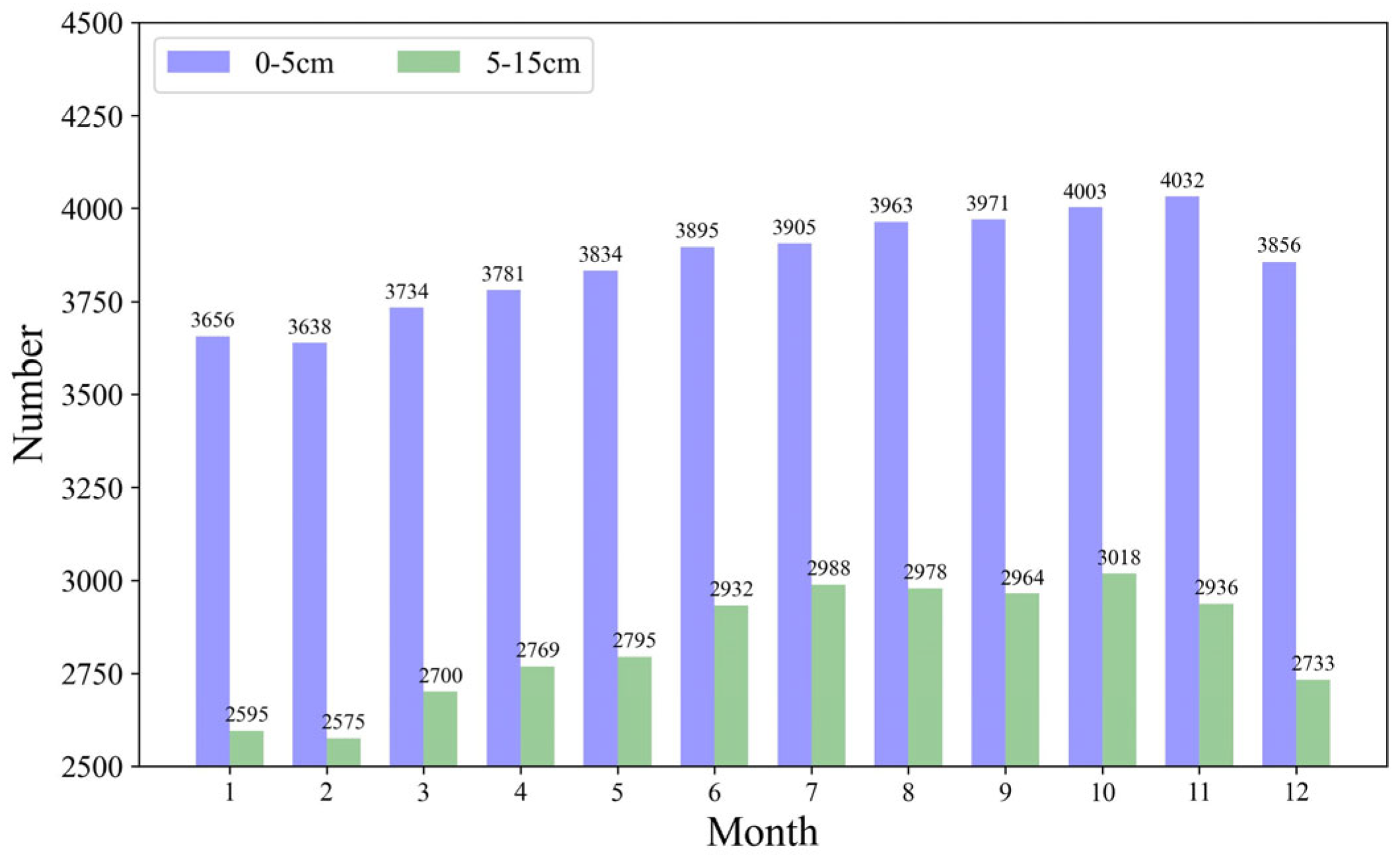
Lembrechts [29] compiled in situ soil temperature measurement data from 9362 independent sensors across 60 countries. Each sensor corresponds to an independent time series, with an average duration of 2.9 years, ranging from 1 month to 41 years, primarily covering the period from 2000 to 2020. In this dataset, all time-series underwent quality control checks, with strict data filtering, for instance, if monthly data contained missing values exceeding one day, such data were excluded. Subsequently, the monthly mean, monthly minimum (5th percentile of all monthly values), and monthly maximum (95th percentile of all monthly values) were calculated. These sensors primarily measured soil temperature at surface (0–5 cm) and subsurface (5–15 cm) depths, with approximately 91% of the data originating from these two depth layers. The collected measurements were averaged into approximately 1200 (surface) and 1000 (subsurface) independent 1 km2 grid cells globally. This study uses data from Lembrechts [29], and given that latitude is a key factor, data from sites located between 30°N and 50°N were selected to align with the geographic scope of the study area, which includes the Huang-Huai-Hai plain (32–40°N). Although the subset corresponding to the Huang-Huai-Hai plain was not reported separately, it lies centrally within the selected latitude range, ensuring that the data is sufficiently representative. The number of available sites for each soil layer, by month, is shown in Figure 2. Both soil layers possess abundant in situ soil temperature data (number of stations), with monthly station numbers ranging from 3638 to 4032 for the shallow layer and 2575 to 3018 for the deep layer. The shallow layer consistently exceeds the deep layer in station numbers by approximately 1000 stations per month across all months.

2.2.2. Predictor Variables

Soil temperature is a parameter regulated by multiple factors, including surface water-heat balance, solar radiation, vegetation cover, and soil properties. Considering this multifaceted influence, this study uses 19 predictor variables, which are categorized into three main groups: environmental variables, soil properties, and topographic factors. The environmental variables included LST [33], evapotranspiration (ET) [34,35], normalized difference vegetation index (NDVI) [36], and shortwave radiation (Reflectance_1, Reflectance_2, Reflectance_3, Reflectance_4, Reflectance_5, Reflectance_6, Reflectance_7) [37]. The soil properties consisted of soil moisture (SM) [38], bulk density, sand content, soil organic carbon (SOC), and soil pH (pH) [39]. The topographic factors included elevation, slope, surface roughness, and the terrain ruggedness index (tri) [40]. The details are presented in Table 1; among these variables, all environmental variables and SM were considered dynamic variables, with data spanning from 2003 to 2020 at a monthly temporal resolution. In contrast, the remaining soil properties and topographic variables were treated as static variables.
Before data utilization, preprocessing was required. The original resolution of bulk density, sand content, SOC, and pH data was 250 m. In this study, these datasets were resampled to 1 km using bilinear interpolation to match the other variables. Additionally, the original ET dataset contained five bands: gross primary production (GPP), total evapotranspiration (Ec), soil evaporation (Es), canopy transpiration (Ei), and ET_water. In this study, ET was calculated as the sum of Ec, Es, and Ei, while the ET_water band was excluded, as the focus was on terrestrial soil temperature.

2.2.3. Auxiliary Variables

Since the focus is the soil temperature variation in cropland, this study used a land cover dataset from Jie Yang [41] to further distinguish cropland from other land cover types. The original resolution of this dataset is 30 m, and it was resampled to 1 km by defining pixels as cropland when they contained at least 2/3 cropland coverage [42]. To ensure comparability across different years, we selected regions that were cropland during the whole period. In addition, previous research has demonstrated that soil type significantly influences soil temperature [43]. Accordingly, 1 km soil type data were obtained from the “1:1,000,000 Soil Map of the People’s Republic of China” published in 1995 by the Resource and Environmental Science Data Platform. For subsequent analysis, the original soil classifications at the Suborder level were aggregated into the Soil Order level.
All datasets used in this study were obtained from publicly accessible and peer-reviewed sources to ensure transparency and reliability. The in situ soil temperature data compiled by Lembrechts et al. underwent strict quality control, including the removal of time series with missing daily records exceeding one day per month and the calculation of monthly mean, minimum, and maximum values. For predictor variables, land surface temperature (LST), evapotranspiration (ET), normalized difference vegetation index (NDVI), and surface reflectance (Reflectance 1–7) were obtained from Zenodo, PML_V2, MODIS MYD13Q1, and MODIS MCD43A4 datasets, respectively. Soil moisture data were derived from the National Tibetan Plateau Data Center, and soil property variables (bulk density, sand content, soil organic carbon, and soil pH) were obtained from the SoilGrids database. Topographic factors including elevation, slope, surface roughness, and terrain ruggedness index were sourced from the EarthEnv Topography dataset. Before modeling, all datasets were preprocessed for spatial consistency by resampling to 1 km resolution and aligning them to a uniform grid. These datasets have been widely used in environmental and climatic studies and provide consistent spatiotemporal coverage from 2003 to 2020, ensuring the reliability of data inputs and the robustness of the model results.

2.3. Methods

2.3.1. Soil Temperature Prediction

Random forest (RF) is an ensemble learning method based on decision trees [44]. It achieves efficient data prediction and classification by constructing a large number of decision trees and aggregating their results through weighted averaging. Due to its significant advantages in handling high-dimensional data, capturing nonlinear relationships, and reducing overfitting, the RF model is widely used in the retrieval of temperature variables [45,46]. Thus, this study employed an RF model to establish monthly relationships between in situ soil temperature and 19 predictor variables. During the construction of the RF model, grid search optimization was performed to determine the optimal configuration among 36 hyperparameter combinations. These hyperparameters included the number of variables considered at each split (ranging from 2 to 10) and the minimum number of samples per leaf node (ranging from 2 to 5). A total of 36 models were generated, each consisting of 250 trees. Model performance was evaluated using k-fold cross-validation (k = 10) during the optimization process. To ensure accurate soil temperature prediction, this procedure was repeated separately for both soil depth layers (0–5 cm and 5–15 cm) for each month, resulting in distinct soil temperature prediction models for each depth layer.
This study involved 19 variables, with varying importance across different seasons. To improve the accuracy and provide a reference for future research on variable selection, the Recursive Feature Elimination with Cross-Validation (RFE-CV) method was adopted. This method incorporates cross-validation into the standard Recursive Feature Elimination (RFE) [47], enabling automatic selection of the optimal feature subset and avoiding model overfitting. RFE-CV is a model-based feature selection technique that iteratively removes features with minimal impact on prediction performance, optimizing the feature set and enhancing the model’s predictive ability. Specifically, the RFE-CV procedure was independently implemented for each month and each soil layer (0–5 cm and 5–15 cm). In each iteration, RFE-CV progressively eliminates unimportant features based on their importance assessment, until the optimal feature subset is identified. This study used the Random Forest Regressor (RandomForestRegressor, n_estimators = 250) as the base estimator, with a step size of 1 (removing one feature per iteration), 5-fold cross-validation, and the coefficient of determination (R2) as the evaluation metric to assess the relationship between the feature subset and the target variable. Ultimately, the RFE-CV method provided the optimal feature subset for model training, improving model prediction performance, reducing feature redundancy, and enhancing computational efficiency, while ensuring the objectivity and reproducibility of the variable selection process.
To comprehensively evaluate the predictive performance of the model, this study employed Mean_R2, Mean_RMSE, Mean_MAE, Mean_NSE, and Mean_Bias (i.e., the average values across multiple trials) to measure the goodness of fit between predicted and observed values. During cross-validation, using these averaged metrics helps to reduce the influence of fluctuations from individual test sets on the evaluation results, thereby enhancing the stability of the assessment. This approach ensured the objectivity and accuracy of the model evaluation, providing a reliable foundation for subsequent soil temperature analysis. It has been widely used in various inversion studies of soil properties [29,48].

2.3.2. Spatiotemporal Variation Analysis of Soil Temperature

To thoroughly analyze the spatiotemporal variation in soil temperature in the croplands of the Huang-Huai-Hai plain, this study was conducted from three perspectives: long-term trends, seasonal characteristics, and depth differences.
Regarding the long-term trends, Sen’s slope estimator [49] and the Mann–Kendall test [50] were employed. The Sen’s slope estimator, a robust non-parametric statistical method for trend estimation, and the Mann–Kendall test, a non-parametric method for assessing time series trend significance, are both suitable for detecting pronounced trends in long-term data. In addition to trend analysis, this study also investigates the fluctuation of soil temperature. Here, the Coefficient of Variation (CV) [51] was used. As a standardized statistical indicator, CV effectively describes the degree of variation in the data relative to its mean, with its formula being:
C V = σ μ × 100 %
where σ represents the standard deviation over the entire study period (2003–2020), measuring the dispersion of the data, and μ denotes the average temperature for the period, reflecting the central tendency of the data.
In terms of analyzing seasonal characteristics, temperature anomalies, rather than soil temperature itself, were used to eliminate the influence of temperature differences across different months. Temperature anomaly is the difference between the observed temperature and the long-term average temperature for the corresponding period, which is defined as:
T = T o b s T a v g
where T represents the temperature anomaly for a certain month, T o b s represents the observed temperature for this month, and T a v g represents the long-term mean temperature for the same month over the study period. The analysis was conducted from two aspects. First, a monthly analysis was performed, including the temporal variation trend and spatial distribution of temperature anomalies. Second, the seasonality of soil temperature was calculated as the difference between the maximum and minimum temperatures within a year, which was also analyzed in terms of both trends and spatial distribution.
Regarding depth differences, the Normalized Cross-Correlation (NCC) [52] was first used to assess the correlation and lag between temperatures at different soil depths. NCC is used to measure the similarity between two soil layers at different lag times. By calculating the cross-correlation coefficient, it is possible to determine whether there is significant synchronous variation between surface temperature and subsurface soil temperature, or whether one time series influences another at a specific time lag. The formula is:
N C C x , y = t = 1 N x t x ¯ y t y ¯ t = 1 N x t x ¯ 2 t = 1 N ( y t y ¯ ) 2
where x t and y t represent the values of the two time-series at time t, x ¯ and y ¯ represent the mean values of time series x and y, respectively, and N is the number of data points. In this study, the lag time was set between 0 and 12 months, and the computed results range from [−1, 1], with positive and negative values indicating positive and negative correlations, respectively. Additionally, the study also analyzed the temporal variation trend and spatial distribution of temperature differences between the two soil layers.
All experiments and analyses in this study were conducted on a computer without the use of laboratory equipment. The only software used was PyCharm Community Edition (version 2022.1.4).

3. Results

3.1. Model Predictive Performance

3.1.1. Model Performance

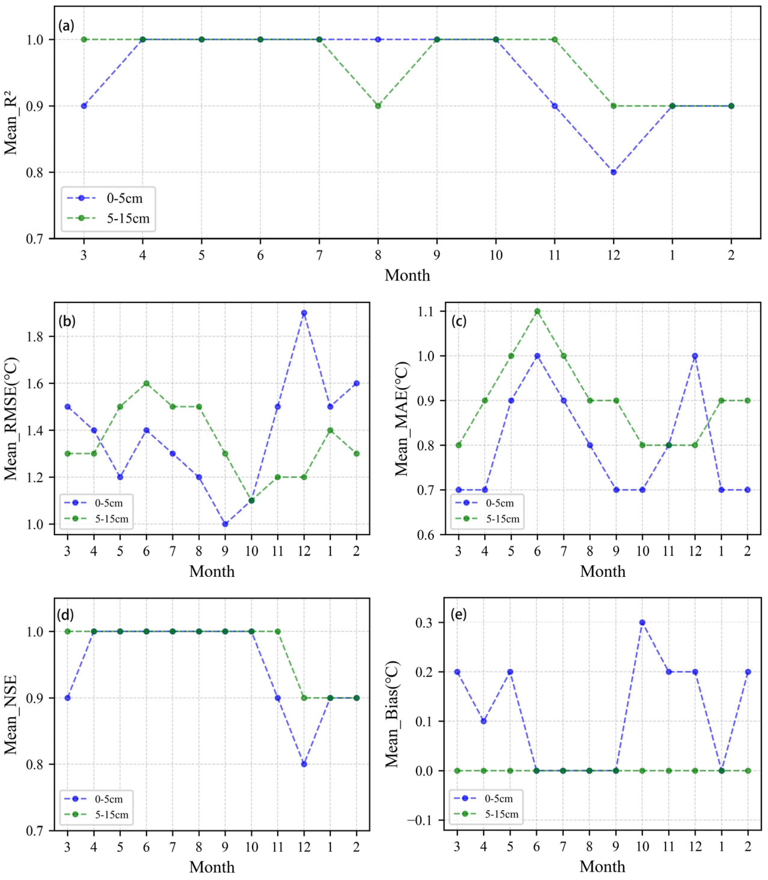
Figure 3 presents the monthly prediction accuracy for soil temperature at two depths, showing high model performance. The Mean_R2 is 0.8–1.0 (0.9–1.0), the Mean_RMSE is 1.0–1.9 °C (1.1–1.6 °C), and the Mean_MAE is 0.7–1.0 °C (0.8–1.1 °C) for the shallow (deep) layer, confirming the effectiveness of the model.
To further illustrate, the 0–5 cm soil layer shows a clear annual pattern in Mean_R2, with the strongest explanatory power in mid-year months and a significant decrease in winter (December to February). Specifically, during spring (March to May), Mean_R2 steadily increases from 0.9 to 1.0, indicating gradually improving model performance. In summer (June to August), Mean_R2 remains stable at the optimal level of 1.0, representing the best performance of the year. In autumn (September to November), it stays at 1.0 in September and October but slightly declines to 0.9 in November. During winter, Mean_R2 drops to its lowest value of 0.8 in December and then slightly recovers to 0.9 in January and February. In comparison, the 5–15 cm layer shows similarly strong performance in spring and early summer, with Mean_R2 maintained at 1.0, consistent with the shallow layer. However, Mean_R2 decreases to 0.9 in August, diverging from the stable trend observed at 0–5 cm. In autumn, it returns to 1.0 and remains stable throughout the season. During winter, Mean_R2 stays at 0.9; although slightly lower than earlier months, the fluctuation is smaller than that of the 0–5 cm layer, indicating better seasonal stability.
The Mean_RMSE for the 0–5 cm soil layer exhibits a clear ‘U’-shaped seasonal variation trend, indicating the necessity of monthly modeling. Specifically, the Mean_RMSE for 0–5 cm follows a complete annual cycle, with higher values in spring and winter, and lower values in summer and autumn. Starting from a peak in winter, the Mean_RMSE gradually decreases, reaching its lowest point in autumn, then quickly rises again in winter, forming a cyclical pattern. In winter, the Mean_RMSE ranges from 1.5 °C to 1.9 °C, representing the highest levels of the year. In spring, it decreases progressively from 1.2 °C to 1.5 °C. During summer, the value gradually declines from 1.4 °C to 1.2 °C, while in autumn, it increases from the lowest point of 1.0 °C to 1.5 °C. Notably, September in autumn has the best prediction performance, with a Mean_RMSE of 1.0 °C, while December in winter has the worst, with the value reaching 1.9 °C. The prediction accuracy at the 5–15 cm depth exhibited seasonal characteristics different from those of the surface layer. Unlike the “U” shaped variation trend observed for the 0–5 cm depth, the Mean_RMSE at the 5–15 cm depth was higher in spring and summer, and lower in autumn and winter. In spring, the value remained between 1.3 °C and 1.5 °C, slightly higher than the range observed for the 0–5 cm depth. As summer approached, the Mean_RMSE further increased to 1.5–1.6 °C, deviating significantly from the 0–5 cm trend, and became the period with the worst prediction performance of the year, particularly in June, when it reached 1.6 °C. Similar to the 0–5 cm depth, the prediction error for the 5–15 cm depth decreased to its lowest point in autumn, ranging from 1.1 °C to 1.3 °C. However, unlike the 0–5 cm depth, where the minimum occurred in September, the lowest value at 5–15 cm was observed in October, at only 1.1 °C, indicating the best prediction performance. In winter, the error stabilized between 1.2 °C and 1.4 °C, noticeably lower than the 1.5–1.9 °C range observed for the 0–5 cm depth in winter, suggesting that the prediction accuracy for the 5–15 cm depth was higher and less fluctuating during winter.
The Mean_MAE for the 0–5 cm layer shows a clear seasonal trend: in spring, it increases from 0.7 °C to 0.9 °C, indicating reduced accuracy toward late spring. During summer, the Mean_MAE decreases steadily from 1.0 °C to 0.8 °C, reflecting continuous improvement in predictive accuracy. In autumn, Mean_MAE reaches its lowest value of 0.7 °C in September and then slightly increases to 0.8 °C by November. In winter, it rises to 1.0 °C in December—the highest value of the year—before decreasing to 0.7 °C by late winter. In comparison, the Mean_MAE for the 5–15 cm layer follows a seasonal trend characterized by higher errors in spring and summer and relatively stable values in autumn and winter. In spring, Mean_MAE increases from 0.8 °C to 1.0 °C, higher than the corresponding values at 0–5 cm. During summer, it ranges between 1.1 °C and 0.9 °C; although slightly decreasing, accuracy remains lower than in the shallow layer. In autumn, Mean_MAE decreases to the lowest levels of the year, with 0.9 °C in September and 0.8 °C in October—the latter representing the best overall performance and outperforming the shallow layer’s minimum. In winter, it fluctuates slightly between 0.8 °C and 0.9 °C, without sharp peaks, showing stronger error control and greater stability than the 0–5 cm layer.
The Mean_NSE for 0–5 cm in spring increased from 0.9 to 1.0, with model accuracy gradually improving. In summer, it remained steady at 1.0, showing the best predictive performance. In autumn, the Mean_NSE stayed at 1.0 from September to October but dropped to 0.9 in November, reflecting the impact of autumnal variations. In winter, it decreased to 0.8 (with the lowest in December), slightly rebounded in January and February, but still remained lower than in other seasons. Compared to the 0–5 cm layer, the 5–15 cm layer maintained a Mean_NSE of 1.0 in both spring and summer, with more stable predictions. In autumn, the Mean_NSE gradually decreased from 1.0 in September to 0.9 in October and November. In winter, it remained stable at 0.9, significantly outperforming the surface layer, indicating that deep soil is less affected by environmental fluctuations.
The Mean_Bias in spring decreased from 0.2 °C in March to 0.1 °C in April, then increased again to 0.2 °C in May, indicating a slight warm bias in late spring. During the summer, the Mean_Bias remained at the ideal level of 0.0 °C, reflecting that the model’s systematic bias was well-controlled. In autumn, September continued to show no bias at 0.0 °C, but in October, it suddenly rose to the highest value of the year, 0.3 °C, showing a significant warm bias, which then decreased to 0.2 °C in November. In winter, January dropped from 0.2 °C to 0.0 °C, reaching the ideal state, while February increased again to 0.2 °C, showing slight fluctuations overall. In contrast, the Mean_Bias for the 5–15 cm layer exhibited remarkable stability and excellent unbiased performance. The Mean_Bias for all months of the year remained at 0.0 °C, with no systematic bias observed across all seasons. This indicates that the model’s prediction for the 5–15 cm layer significantly outperforms the surface layer in controlling systematic errors, showing higher predictive reliability and stability, unaffected by seasonal variations.

3.1.2. Feature Importance

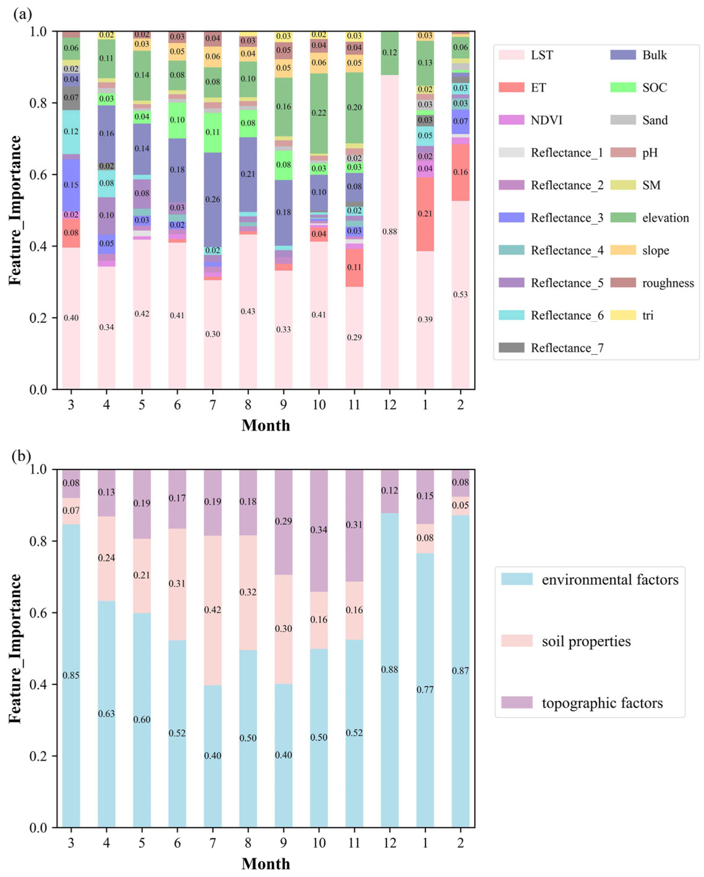
After analyzing the model accuracy, the study further examined the influence of different variables on the 0–5 cm soil temperature. To clearly illustrate seasonal variations, the variables were combined and analyzed into three categories: environmental variables, soil properties, and topographic factors, as shown in Figure 4. The results confirmed that soil temperature is influenced by the combined effect of these three categories of factors, consistent with the findings of Z. Feng [53]. The analysis revealed that the importance of these three factors exhibited distinct seasonal variations. Specifically, environmental variables showed a “decrease-then-increase” trend, with higher contributions in spring and winter (ranging from 0.6 to 0.88), and relatively lower values in summer and autumn (ranging from 0.4 to 0.52). In contrast, the contributions of soil properties and topographic factors exhibited an “increase-then-decrease” trend. Soil properties contributed less in spring and winter (ranging from 0 to 0.24), but significantly increased in summer and autumn, reaching values between 0.16 and 0.42. Topographic factors contributed between 0.08 and 0.19 in spring and winter, and increased to 0.17 to 0.34 in summer and autumn. This complementary seasonal interplay among environmental variables, soil properties, and topographic factors may stem from the following: in spring and winter, low temperature and humidity enhance the importance of environmental variables such as LST and reflectivity; in summer, high temperature and humidity promote microbial activity and nutrient release, strengthening soil properties; and in autumn, topographic factors gain prominence due to their influence on localized water and nutrient distribution, such as retention or loss. As shown in Figure 4a, among the environmental variables, LST consistently showed high contributions throughout the year, fluctuating between 0.29 and 0.88. It reached its highest value of 0.88 in December during winter, while it dropped to its lowest point of 0.29 in November during autumn, exhibiting a distinct seasonal fluctuation. ET had a more significant impact in late autumn, winter, and early spring, with the highest contribution of 0.21 in January, second only to LST within the environmental variables. Additionally, Reflectance_3 had the most notable influence in early spring, with a contribution of 0.15. Among the soil properties, Bulk density played a dominant role, and along with SOC, its contribution increased significantly in summer and early autumn, reaching the highest values of 0.26 and 0.11, respectively, in July. Among the topographic factors, elevation had the most significant contribution throughout the year, with the highest value of 0.22 in October during autumn.
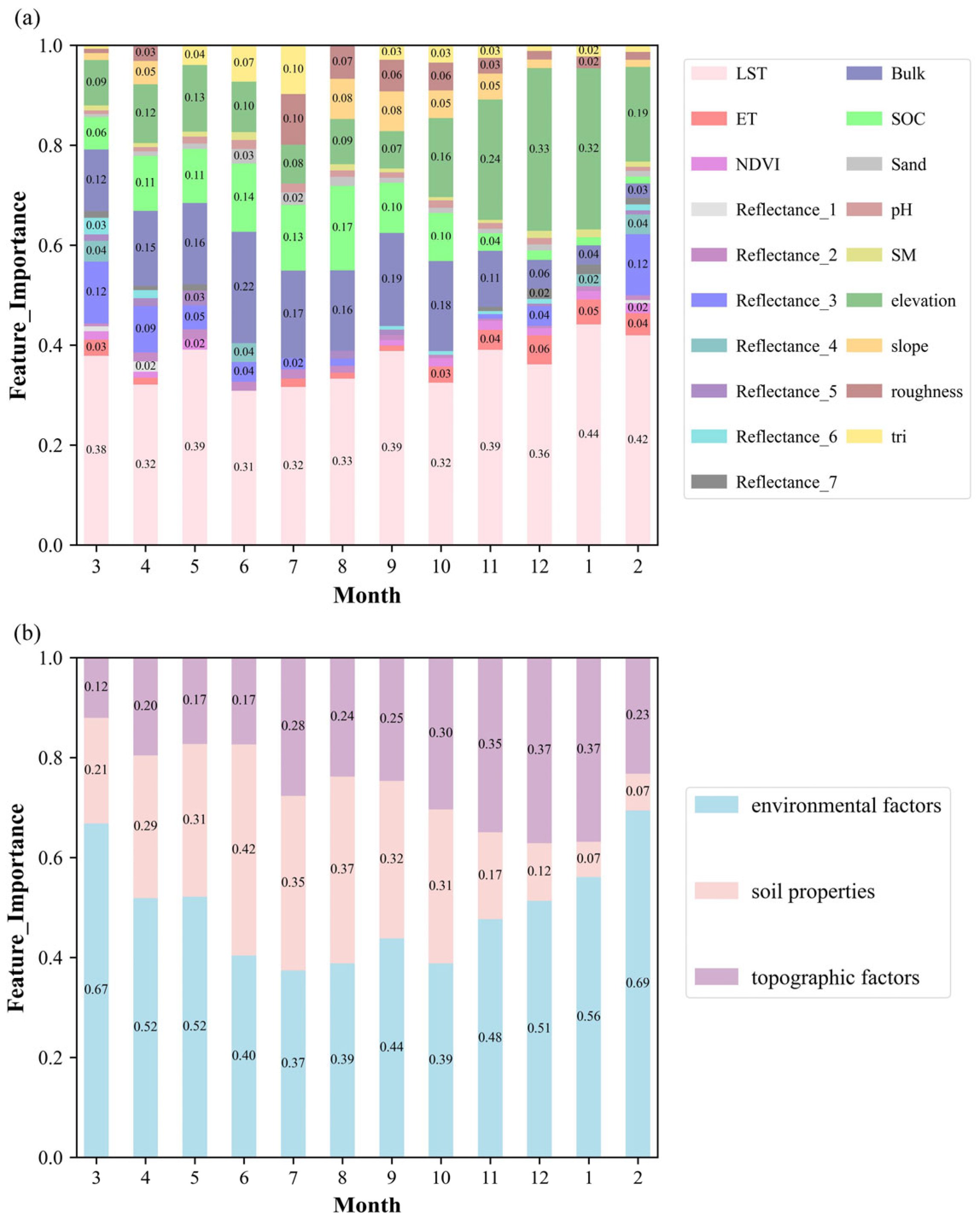
Similarly to prediction accuracy, the feature importance at the 5–15 cm soil depth also exhibited a pattern distinct from the surface layer, as shown in Figure 5b. With increasing soil depth, the dependence on environmental variables generally decreased, while the reliance on soil properties and topographic factors increased. For deeper soils, the influence of topographic factors became particularly significant and should not be overlooked. Specifically, compared to the 0–5 cm depth, the environmental variables for the 5–15 cm depth still displayed a “decrease-then-increase” trend, but with a lower overall contribution. In spring and winter, the contribution ranged from 0.51 to 0.69, while in summer and autumn, it decreased to 0.37 to 0.48, with smaller fluctuations. Soil properties also showed an “increase-then-decrease” trend, but with an increased contribution range in spring and winter (0.07–0.31), while the contribution range in summer and autumn (0.17–0.42) was similar to the 0–5 cm depth. The trend for topographic factors was distinctly different, showing a continuous increase from spring and summer (0.12–0.28) to autumn and winter (0.23–0.37), likely due to the growing seasonal cumulative effect of topography on deep-layer water and nutrient retention. As shown in Figure 5a, LST remained the highest contributing variable among the environmental variables, but it fluctuated more smoothly throughout the year, with the contribution range narrowing to 0.31–0.44. The highest value occurred in January (0.44), and the lowest value in June (0.31). The influence of ET at the 5–15 cm depth was relatively weak, with the highest contribution of only 0.06 in December, indicating that ET has a limited role in deeper soils. The impact of reflectance_3 at this depth was concentrated mainly in late winter and early spring, with the highest contributions in February and March (0.12). Regarding soil properties, Bulk density remained the dominant factor at 5–15 cm, but the role of SOC became more prominent. SOC reached a contribution of 0.17 in July, surpassing Bulk density and becoming the most significant factor for soil properties during that season. In contrast, the peak contribution of Bulk density occurred in June (0.22), slightly earlier than the highest contribution of SOC. As for topographic factors, the contribution of elevation at the 5–15 cm depth steadily increased, reaching its highest value in December (0.33), indicating that elevation had a more pronounced influence on deeper soils during the winter.

3.2. Spatiotemporal Patterns of Soil Temperature

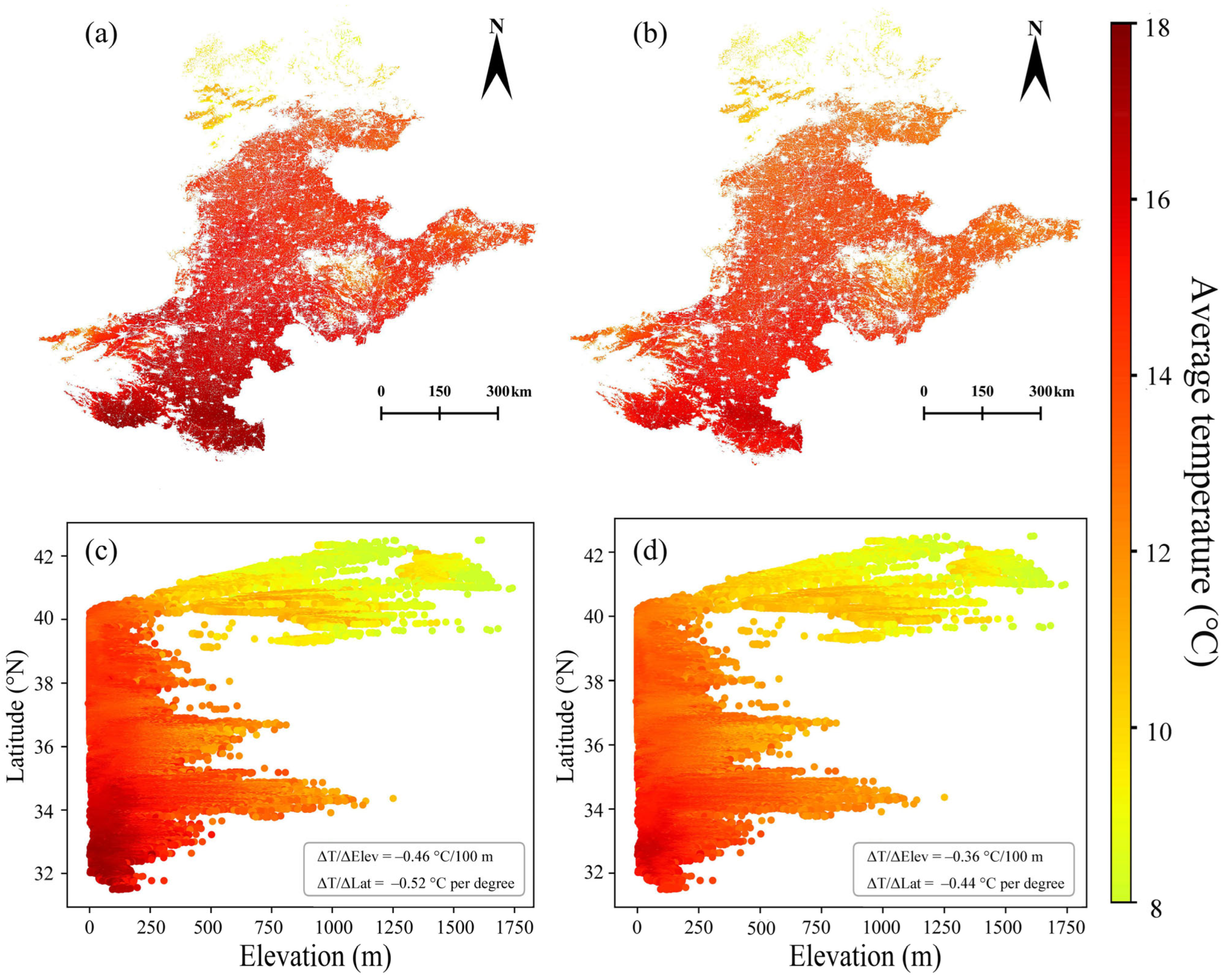
Based on the optimal variables identified for each month, we collected the relevant data and applied the RF model to generate 0–5 cm and 5–15 cm soil temperature data for the Huang-Huai-Hai plain at a 1 km resolution from 2003 to 2020. This study focused on cropland analysis; thus, only cropland data were extracted, and the spatial distribution of the 18-year average values was calculated, as shown in Figure 6. The analysis revealed that the spatial distribution of soil temperatures in both soil layers was primarily influenced by latitude and elevation. To further investigate this, we plotted the relationship between soil temperature and both latitude and elevation (subplots c and d). The results indicate that, except for areas with high latitude and high elevation, the 0–5 cm soil temperature is generally higher than the 5–15 cm soil temperature. Despite the temperature differences, the spatial distribution patterns of the two soil layers exhibit similar regional characteristics: Higher latitudes correspond to lower temperatures, while at the same latitude, higher elevations are associated with lower temperatures. Specifically, the 0–5 cm soil temperature decreases by 0.46 °C for every 100 m increase in elevation and by 0.52 °C for every 1° increase in latitude; the 5–15 cm soil temperature decreases by 0.36 °C for every 100 m increase in elevation and by 0.44 °C for every 1° increase in latitude.
This spatial distribution characteristic provides a foundation for understanding soil temperature variation. However, analysis based solely on the average state is insufficient to reveal the complete variation pattern. To comprehensively understand the spatiotemporal changes in cropland soil temperature from 2003 to 2020, this study examines three aspects: annual scale (long-term trends), intra-annual scale (seasonal characteristics), and intrinsic soil properties (depth differences).

3.2.1. Long-Term Trend Analysis

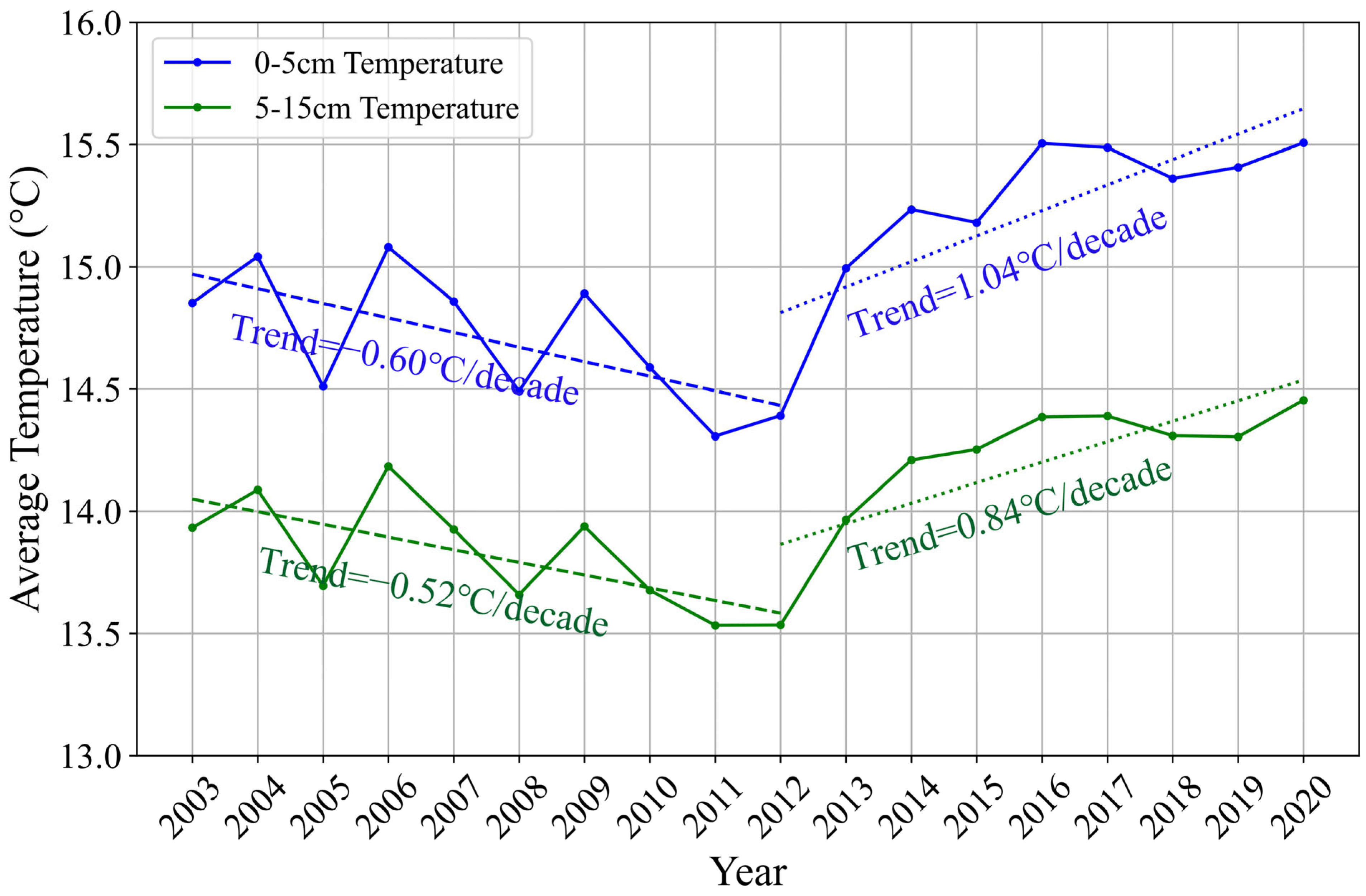
Figure 7 illustrates the variation trends of average temperature for the 0–5 cm and 5–15 cm soil layers over 18 years. The results show that soil temperature in cropland of the Huang-Huai-Hai plain exhibited an overall warming trend from 2003 to 2020, consistent with the findings of García-García [54]. Building on this, further analysis reveals that both soil layers displayed a phased pattern of initial cooling followed by warming, with the shallow layer being more sensitive to temperature changes. Specifically, the annual average temperature for the 0–5 cm (5–15 cm) layer decreased from 2003 to 2012 by −0.6 °C/decade (−0.52 °C/decade), while it increased from 2012 to 2020 by 1.04 °C/decade (0.84 °C/decade).
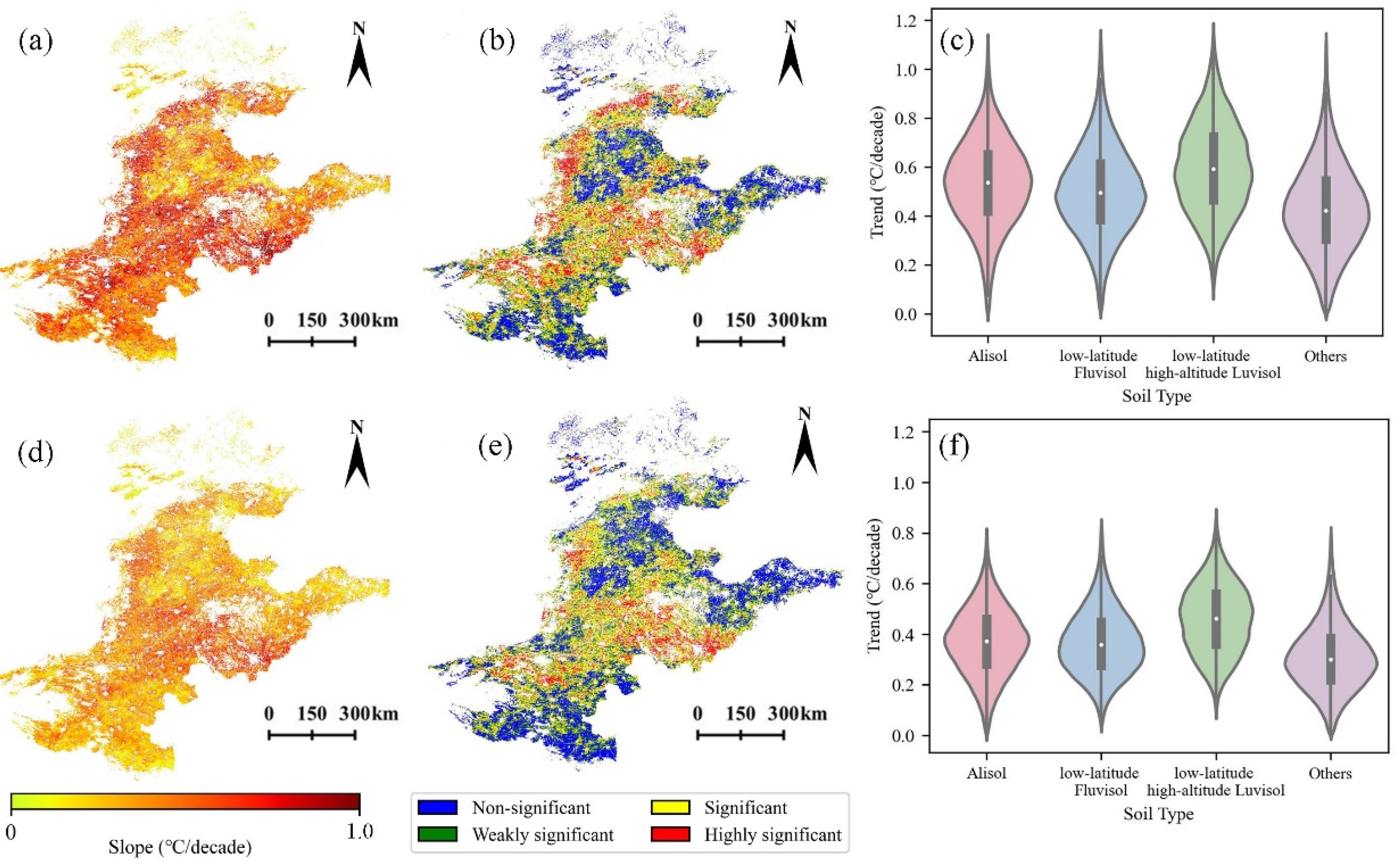
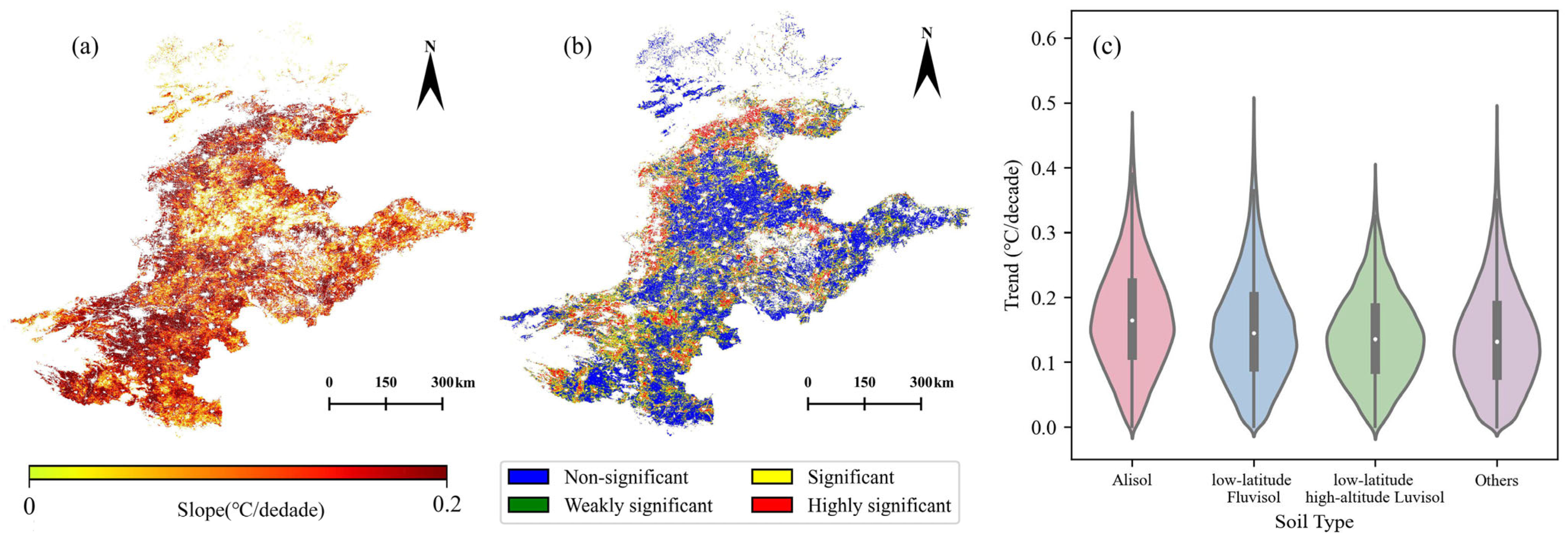
To further understand the spatial heterogeneity of this temperature change, Figure 8 illustrates the spatial distribution of the trends. As shown in subplots b and d, over the past 18 years, the statistical significance of soil temperature changes at the 0–5 cm (5–15 cm) depth was as follows: highly significant in 17.14% (11.29%), significant in 38.60% (36.46%), weakly significant in 16.72% (19.19%), and non-significant in 27.54% (33.07%), indicating that the results are statistically meaningful. Trend analysis revealed that the area with a positive slope for the 0–5 cm (5–15 cm) soil layer accounted for as high as 99.19% (99.49%), which led us to focus on the warming areas. As shown in subplots a and c, Sen’s slope was primarily distributed between 0 °C/decade and 1.0 °C/decade, indicating a general upward trend in soil temperature. However, there was a notable vertical difference, with the shallow soil warming faster than the deeper soil. Considering the impact of soil type [43], we further integrated the data from Figure 1d and found that the rate of change is closely related to soil types. Specifically, in Alisol, low-latitude Fluvisol, and low-latitude–high-altitude Luvisol, the warming rate significantly increased, while it was slower in other soil types. To visually illustrate these differences, we generated violin plots (subplots e and f), noting that all violin plots in this study are based on data within the 0.1–99.9% percentile range to exclude extreme outliers. In detail, the median warming trend for Alisol at 0–5 cm (5–15 cm) was 0.54 °C/decade (0.37 °C/decade), for low-latitude Fluvisol was 0.49 °C/decade (0.36 °C/decade), and for low-latitude–high-altitude Luvisol was 0.59 °C/decade (0.46 °C/decade), all higher than the 0.42 °C/decade (0.30 °C/decade) for other soil types.
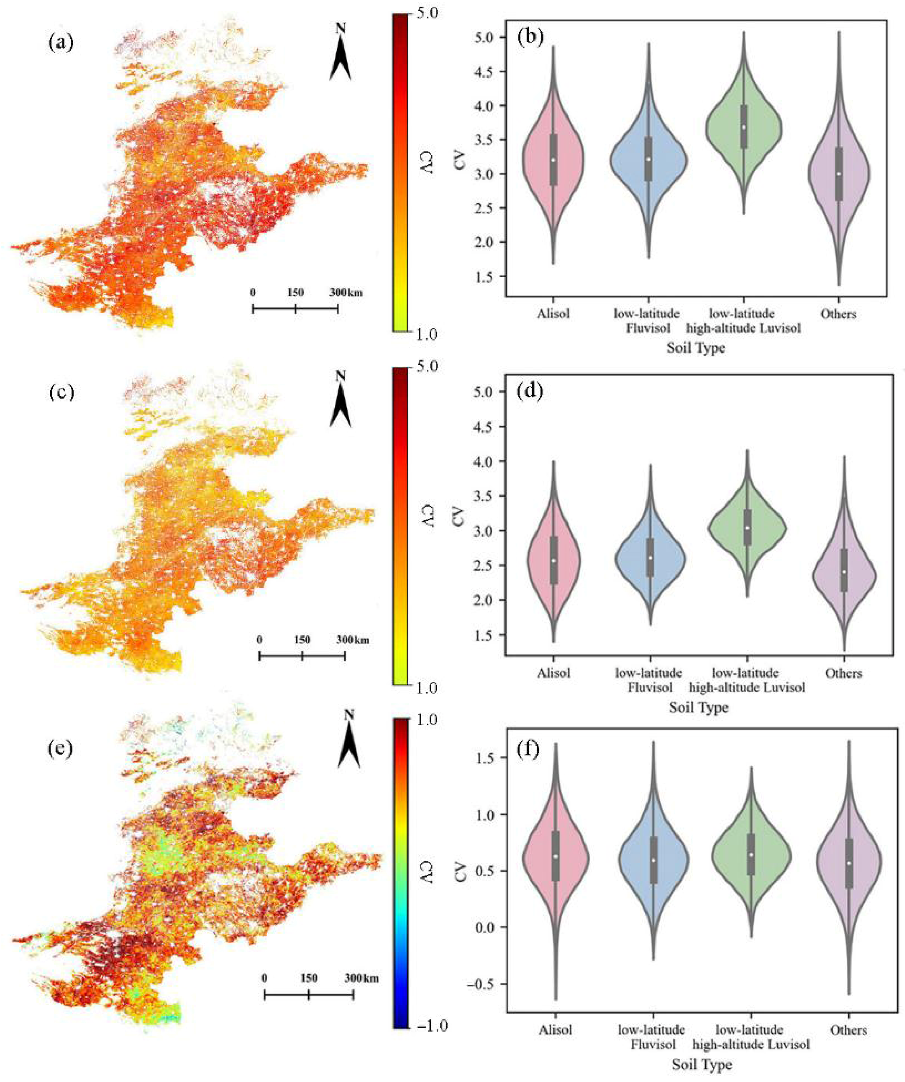
To assess the temperature fluctuations in different regions, this study calculated CV of temperature over multiple years (Figure 9). As shown in subplots a and b, similar variability patterns were observed across different soil layers. Regions dominated by Alisols, low-latitude Fluvisols, and low-latitude–high-altitude Luvisols exhibited higher coefficients of CV, indicating greater temperature fluctuations, whereas other soil types showed relatively lower CVs, reflecting more stable thermal conditions. Specifically, the median CV at 0–5 cm (5–15 cm) was 3.20 (2.57) for Alisol, 3.21 (2.61) for low-latitude Fluvisol, and 3.68 (3.04) for low-latitude–high-altitude Luvisol, compared to 3.00 (2.41) for other soil types. A further comparison between soil layers (subplots e and f) revealed that temperature fluctuations were generally more pronounced in the 0–5 cm layer than in the 5–15 cm layer. However, due to soil type influences, some regions, excluding the aforementioned three soil types, exhibited the opposite pattern.

3.2.2. Seasonal Characteristics Analysis

Figure 10 illustrates the temperature anomalies in different soil layers across various seasons, revealing an overall upward trend in soil temperature with significant seasonal differences. To characterize this trend, we used 2011 as a temporal breakpoint and calculated seasonal mean temperature anomalies by averaging deviations from the multi-year mean for the periods 2003–2011 and 2012–2020. Results demonstrate a consistent warming pattern across seasons and soil depths. In spring, the mean anomaly increased from −0.5 °C to 0.5 °C at the 0–5 cm depth and from −0.4 °C to 0.4 °C at the 5–15 cm depth; in summer, anomalies rose from −0.4 °C to 0.4 °C (0–5 cm) and from −0.2 °C to 0.2 °C (5–15 cm). A smaller increase was observed in autumn, with both depths shifting from −0.1 °C to 0.1 °C, while winter temperatures remained largely stable with anomalies close to 0 °C across both layers. Notably, negative anomalies dominated the earlier period (2003–2011), whereas positive anomalies became prevalent after 2011, marking a distinct temporal shift consistent with the warming signal shown in Figure 6. In addition, several extreme outliers are evident in Figure 9, such as the substantial cooling observed in the 0–5 cm layer during the summer of 2008 (−1.9 °C anomaly) and the anomalous winter warming in 2020, when anomalies reached 2.0 °C and 1.8 °C in the 0–5 cm and 5–15 cm layers, respectively. However, these sporadic extremes did not alter the overall trajectory of progressive warming.
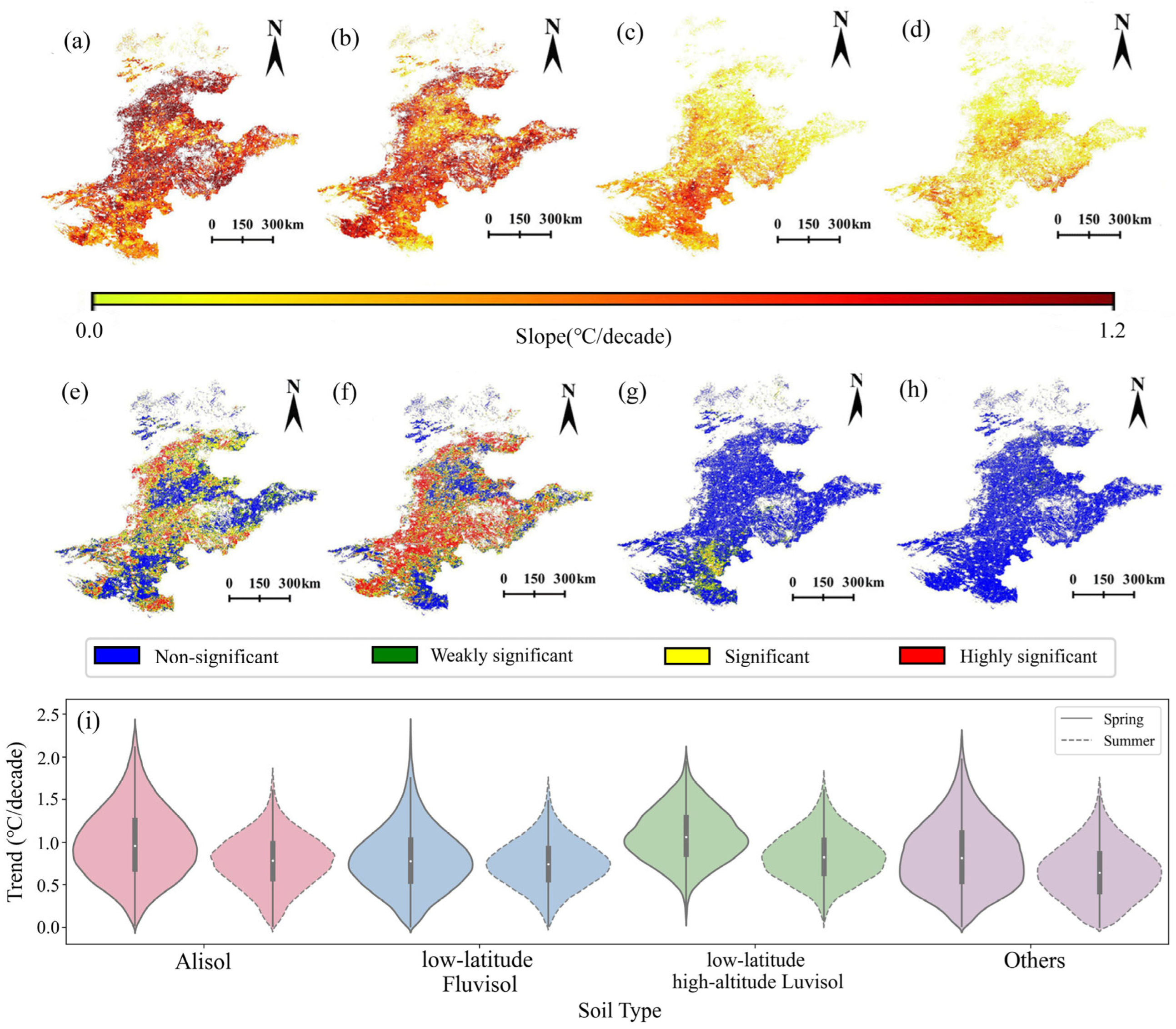
To further investigate the spatial distribution of temperature anomalies, Figure 11 presents the seasonal trends in the 0–5 cm soil layer based on Sen’s slope analysis. The figure primarily highlights regions exhibiting a positive slope, as areas with negative trends are minimal—accounting for only 1.56% in spring, 1.95% in summer, 19.15% in autumn, and 27.53% in winter. Although the proportion of negative trends increases slightly in autumn and winter, the corresponding slope magnitudes remain small, indicating limited influence on the overall warming pattern. The results show that the temperature anomaly trends exhibit certain seasonality and are closely related to soil type. The 0–5 cm soil temperature has exhibited a warming trend over the past 18 years, with Alisol, low-latitude Fluvisol, and low-latitude–high-altitude Luvisol showing the most pronounced warming in spring and summer, characterized by high Sen’s slopes and mostly highly significant or significant MK test outcomes. As shown in subplot i, for spring (summer), the median warming rate was 0.96 °C/decade (0.78 °C/decade) for Alisol, 0.78 °C/decade (0.74 °C/decade) for low-latitude Fluvisol, and 1.06 °C/decade (0.82 °C/decade) for low-latitude–high-altitude Luvisol. Except for low-latitude Fluvisol in spring, these rates exceed other soil types at 0.81 °C/decade (0.64 °C/decade). In contrast, warming trends in most regions during autumn and winter are generally moderate, with smaller Sen’s slopes and mostly non-significant or weakly significant MK test results.
Compared to the 0–5 cm layer, the temperature anomaly trend for the 5–15 cm soil layer also showed an overall warming trend across the four seasons (Figure 12, with details as described earlier, only analyzing areas with a positive Sen’s slope, which accounted for 99.02% in spring, 98.81% in summer, 78.53% in autumn, and 69.73% in winter), but the changes are more gradual, with the Sen’s slopes for each season generally smaller than those at 0–5 cm. The deep soil layer exhibits a similar warming trend in spring and summer. Specifically, as shown in subplot i, for spring (summer), the median warming rates were 0.72 °C/decade (0.50 °C/decade) for Alisol, 0.59 °C/decade (0.42 °C/decade) for low-latitude Fluvisol, and 0.84 °C/decade (0.58 °C/decade) for low-latitude–high-altitude Luvisol. Similar to the 0–5 cm layer, except for low-latitude Fluvisol in spring, all these rates exceed those observed in other soil types, which averaged 0.60 °C/decade in spring and 0.42 °C/decade in summer. However, the intensity of warming is weaker than that of the shallow soil. Notably, in the MK test for summer, the range of highly significant areas at 5–15 cm is broader than at 0–5 cm, suggesting that although the temperature variation in deep soil during summer is smaller, it shows greater statistical stability. In autumn and winter, both soil layers show similar patterns, dominated by non-significant changes.
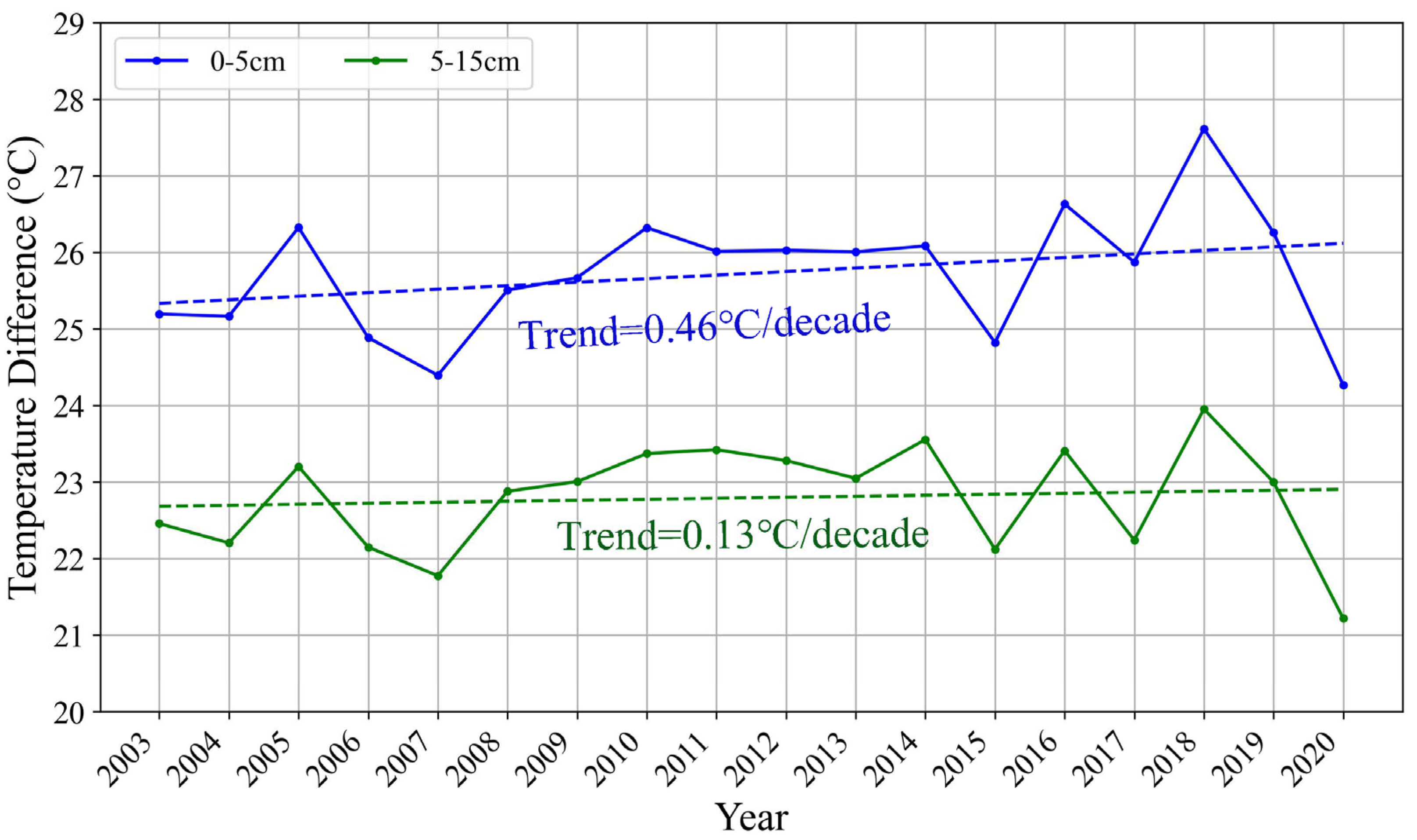
In addition to changes in temperature anomalies, the evolution of seasonal temperature differences merits attention. Figure 13 illustrates the maximum monthly temperature difference for each year, analyzing seasonality trends over the past 18 years. The results indicate that the soil temperature variation at 0–5 cm depth ranges from 24.27 to 27.62 °C, while that at 5–15 cm depth ranges from 21.22 to 23.96 °C. This suggests that temperature differences at 0–5 cm are consistently greater than those at 5–15 cm, with an average difference of approximately 3 °C and more pronounced fluctuations. Furthermore, temperature differences at both depths exhibit an upward trend. However, the shallow layer displays greater variability in temperature differences, with an increase rate of 0.46 °C/decade, whereas the deeper layer remains relatively stable, with a lower overall increase rate of 0.13 °C/decade. Notably, in 2019 and 2020—particularly in 2020—the overall temperature rose [55,56] while seasonality diminished [57,58,59], indicating that the temperature increase in colder months exceeded that in warmer months.
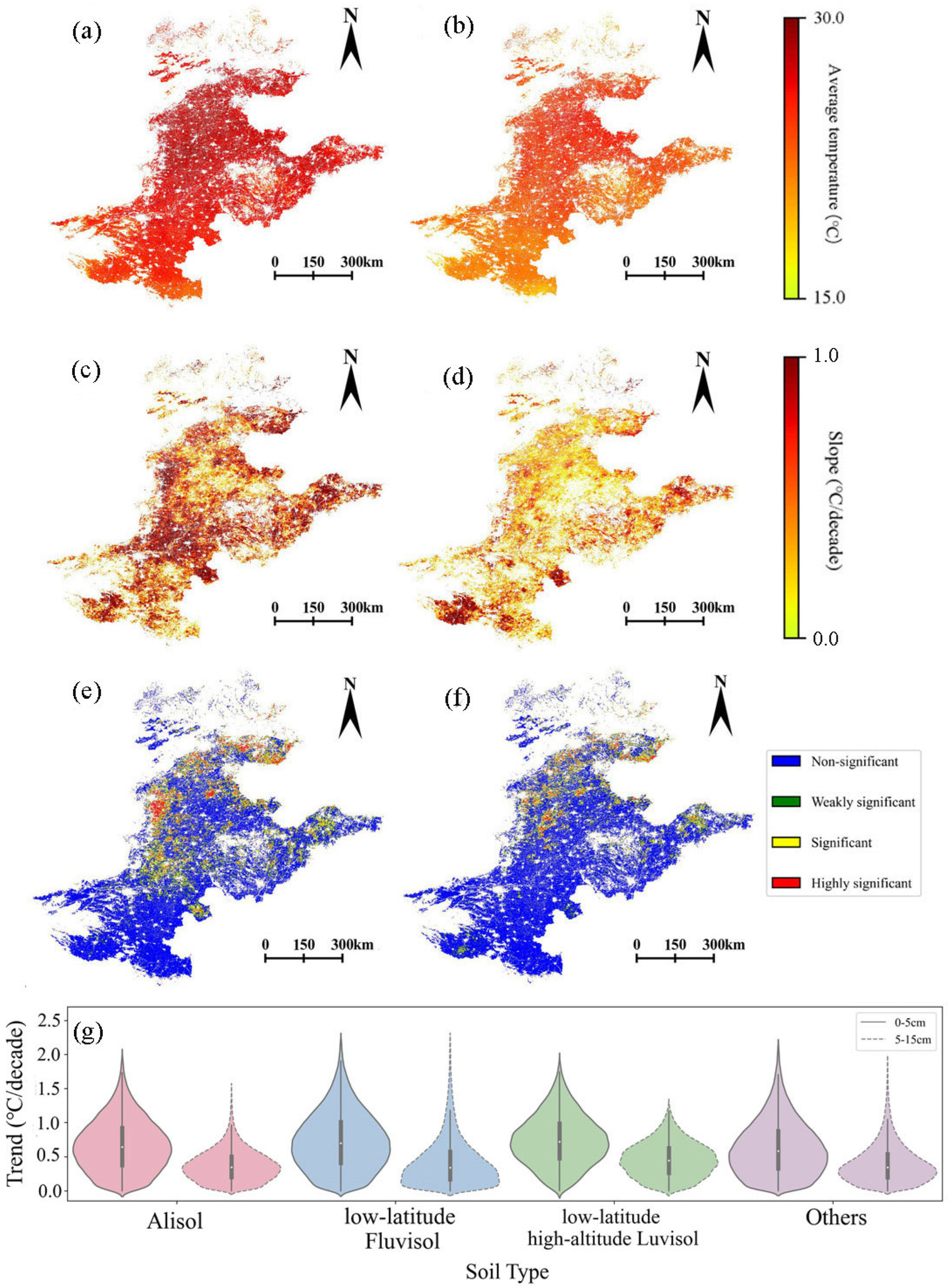
To understand the regional influences behind these differences, we examined their spatial patterns (Figure 14). Consistent with previous analyses, only regions with positive Sen’s slopes were analyzed, as negative slopes, though notable (14.3% for 0–5 cm; 22.74% for 5–15 cm), have generally low absolute values. The spatial distribution shows that temperature fluctuations in the 0–5 cm soil layer are more pronounced than in the 5–15 cm layer. Both layers exhibit similar spatial patterns: on average, soils in the 35–40°N region have shown substantial temperature differences over time, with significant fluctuations. The temperature difference generally increases, with Alisol, low-latitude Fluvisol, and low-latitude–high-altitude Luvisol showing faster rates of increase, while other regions remain relatively stable. As shown in subplot g, for 0–5 cm (5–15 cm) soil layers, the median warming rate was, for Alisol, 0.64 °C/decade (0.35 °C/decade); low-latitude Fluvisol, 0.69 °C/decade (0.34 °C/decade); low-latitude–high-altitude Luvisol, 0.72 °C/decade (0.44 °C/decade). In contrast, other regions have milder warming rates of 0.58 °C/decade (0.34 °C/decade).

3.2.3. Depth Variation Analysis

The analyses in the previous two sections indicate that both long-term trends and seasonal characteristics are more stable in deeper soil layers than in shallow ones. This subsection further provides a more detailed examination of the temporal correlation between the two soil layers and the spatial distribution of temperature differences.
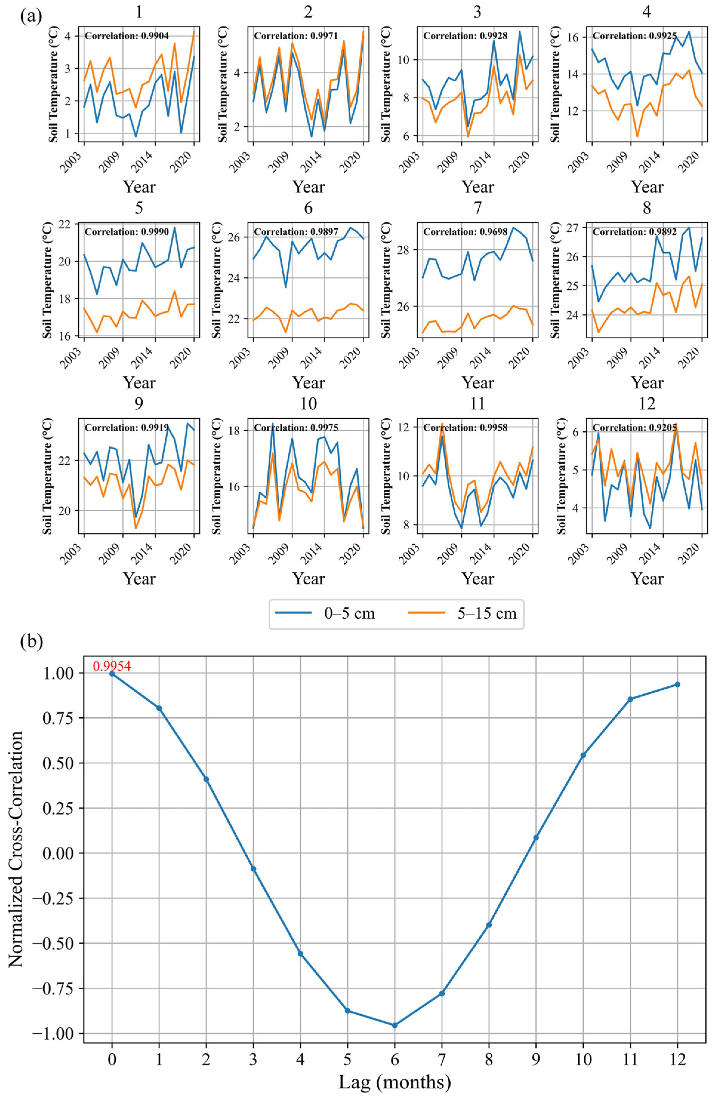
Figure 15a analyzes the correlation of monthly soil temperatures between the two soil layers and shows that, despite differences in the monthly variation patterns, the two layers exhibit similar trends with a very strong correlation ranging from 0.9205 to 0.9990. Given this strong correlation, we further investigated whether there is any lag effect between the two soil layers (Figure 15b). The results indicate that the correlation peaks at zero lag (0 months) with a value of 0.9954 and gradually diminishes as the lag in months increases. Therefore, it can be concluded that there is no significant lag effect between the temperature changes in the two layers. The temperature changes in both depths occur nearly simultaneously, with heat being transferred very quickly between the two soil layers, almost exhibiting synchronous variation.
At the spatial level, the study calculated the temperature difference between the 5–15 cm and 0–5 cm soil layers. Generally, a larger (smaller) temperature difference indicates lower (stronger) soil thermal inertia. Figure 16 illustrates the spatial distribution of the temperature difference trends between the two soil layers (with Sen’s slope calculation details consistent with previous sections, focusing on the positive slope portion, which accounts for 92.32%). The results reveal significant variations in temperature difference changes between the two layers, largely influenced by soil type. Specifically, as shown in subplot c, Alisol (median rate of 0.16 °C/decade), low-latitude Fluvisol (0.14 °C/decade), and low-latitude–high-altitude Luvisol (0.14 °C/decade) exhibit the most pronounced increasing trends in temperature differences. These regions not only show faster rates of increase but also demonstrate high statistical significance (significant or highly significant), indicating a rapid reduction in thermal inertia. In contrast, other regions also display an increasing trend in temperature differences (median rate of 0.13 °C/decade), but the rates of increase are lower, and most areas do not reach statistical significance, suggesting a slower reduction in thermal inertia in these regions.

4. Discussion

4.1. Model Development and Feature Selection Strategy

Compared with previous studies that relied on a limited set of variables [8,11,24], this study incorporated 19 geo-environmental variables—including environmental variables, soil properties, and topographic factors—providing more comprehensive and multidimensional input features for the model, thereby enhancing its responsiveness to soil temperature variations. Additionally, approximately 3000 in situ soil temperature measurements were employed, with observation sites distributed across latitudes from 30°N to 50°, ensuring strong spatial representativeness. Specifically, no fewer than 3638 valid observations were available for the 0–5 cm soil layer and 2575 for the 5–15 cm layer, offering a solid data foundation for constructing depth-specific models and effectively ensuring the accuracy and reliability of the predictions.
Beyond model construction, this study further focused on evaluating the importance of input variables—an aspect often overlooked in previous research [28,60,61]. A soil temperature prediction model was developed, and the seasonal dynamics of variable importance were thoroughly analyzed. The study found that the importance of the variables for prediction exhibited clear seasonal variations. For example, LST and Reflectance_3 showed a “decrease-then-increase” pattern, while SOC and bulk density followed an “increase-then-decrease” trend. Furthermore, these seasonal patterns significantly varied with soil depth; for instance, elevation in deeper soil layers exhibited a continuous growth trend opposite to that observed in the surface layers. These findings provide scientific support for variable selection in soil temperature models and offer valuable insights for the design of future observational experiments and quantitative analysis methods.

4.2. Seasonal Mechanisms of Predictive Factors

The higher contribution of environmental variables in spring and winter may be attributed to the dominant role of surface radiation and atmospheric forcing during cold seasons, when vegetation cover and soil moisture are relatively low, which together enhance the direct influence of land surface temperature (LST) on soil heat exchange [62]. In contrast, during summer and autumn, stronger vegetation growth and evapotranspiration alter the surface energy balance and increase latent heat flux, thereby weakening the control of environmental variables on soil temperature. The greater importance of soil properties in these warmer seasons likely results from enhanced microbial and physical processes that modify bulk density and soil organic carbon (SOC), which in turn affect soil thermal conductivity and heat capacity, allowing the soil to buffer temperature fluctuations more effectively [63,64]. The increasing influence of topographic factors toward winter, especially elevation, reflects their cumulative effects on water retention and heat redistribution, which regulate subsurface thermal conditions over time [65]. It was observed that the temperature variation in winter was relatively smaller than in other seasons. This phenomenon is likely caused by the combined effects of soil thermal inertia and freeze–thaw processes. The high heat capacity of deeper soil layers results in slower temperature responses to atmospheric fluctuations, while frozen layers act as insulating barriers that suppress vertical heat exchange between the soil and the atmosphere [66]. These mechanisms collectively explain the attenuated seasonal amplitude of soil temperature during the winter months.

4.3. Spatial Variation in Soil Temperature Dynamics and Contributing Factors

In all analyses (long-term trends, interannual variations, seasonality, and vertical comparisons), Alisol, low-latitude Fluvisol, and low-latitude–high-altitude Luvisol consistently exhibit stronger warming rates and greater temperature variability than other soil types, with the low-latitude–high-altitude Luvisol showing the highest median slope. We attribute these differences to variations in climate, soil texture, and moisture conditions. Specifically, Alisol, due to their low soil permeability and variable moisture conditions, often exhibit more pronounced seasonal surface temperature responses [67]. The low-latitude Fluvisol, typically found in areas with strong solar radiation and low soil moisture, can enhance soil heat input and reduce thermal buffering, leading to faster warming. The low-latitude–high-altitude Luvisol is influenced by the combined effects of increased radiation and limited moisture, resulting in higher effective thermal conductivity and faster warming [68]. These factors collectively contribute to the stronger warming rates and greater temperature variability observed in these soil types, providing further insights into the spatial variation in soil temperature dynamics.

4.4. Impact of Soil Temperature on Crop Growth Stages

In the Huang-Huai-Hai Plain, soil temperature dynamics are closely related to the growth cycles of the region’s dominant crops—winter wheat and summer maize. Warmer soil conditions in early October favor wheat sowing and emergence, while springtime warming accelerates green-up and jointing [69]. During June–July, when summer maize is sown, higher shallow-layer temperatures promote rapid germination and seedling establishment [70]. However, the intensified warming observed in summer may increase evapotranspiration during the maize filling stage, highlighting the need for precise irrigation management. The quantified soil-temperature gradients with elevation and latitude further suggest that cooler conditions at higher elevations or northern areas could delay crop development, emphasizing the value of localized sowing-time adjustment. These findings demonstrate that the high-resolution soil-temperature dataset developed in this study can directly support phenology-aware precision agriculture across the Huang-Huai-Hai Plain.

4.5. Limitations and Future Directions

This study employed an RF model with RFE-CV to predict soil temperature at depths of 0–5 cm and 5–15 cm. The results indicate that this method demonstrates strong robustness in predicting temperatures at different soil depths. However, despite the identification of important variables, there are still some limitations. Firstly, although the RF model shows high stability, it relies on limited observational site data, which increases uncertainty when extrapolating to unsampled areas [71], especially in regions with complex topography, diverse soil types, or unique climatic conditions. This may affect the reliability and accuracy of the model at regional scales. Secondly, the model was developed using all land cover types, yet this study focused solely on cropland data; optimizing the model specifically for cropland could further enhance prediction accuracy and applicability. Additionally, in our current study, only the soil temperature predictions for 0–5 cm and 5–15 cm were conducted. However, deep soil temperature also holds significant research value for cropland [72]. Crop root systems typically extend into deeper soil layers, and deep soil temperature has a significant impact on water absorption and nutrient utilization efficiency during crop growth and development. To address the above limitations, future research should focus on three main directions. First, to reduce the uncertainty caused by limited in situ observations, it is necessary to expand the monitoring network and integrate multi-source data, such as reanalysis products and high-resolution remote sensing, to improve spatial coverage and model generalization through spatially blocked cross-validation or transfer learning techniques. Second, model optimization should consider different land cover types. Building and comparing land-cover-specific models (e.g., cropland, grassland, and forest) could better reflect the distinct thermal and hydrological characteristics of each ecosystem, thereby improving applicability and interpretability. Third, extending the modeling framework to deeper soil layers (e.g., 30–100 cm) using multi-depth coupling or hierarchical modeling approaches would enable a better understanding of vertical heat transfer processes and soil–crop interactions across profiles. These methodological extensions will help enhance the spatial reliability, physical interpretability, and long-term predictive capability of soil temperature models.

5. Conclusions

To achieve high-accuracy estimation of soil temperature in agricultural regions, this study developed an enhanced RF modeling framework. The model was built using approximately 3000 in situ soil temperature samples from 2003 to 2020, combined with 19 multi-source geo-environmental variables. LST was used in place of traditional air temperature, and RFE-CV was applied to optimize variable selection. Monthly models were constructed separately for the 0–5 cm and 5–15 cm soil layers, enabling high-precision prediction at a 1 km spatial resolution. Based on this, a monthly soil temperature dataset was generated for croplands in the Huang-Huai-Hai plain, which features a typical temperate monsoon climate and intensive agricultural activity. Based on this representative region, model performance was evaluated, and a systematic analysis was conducted on the spatiotemporal variation in soil temperature in terms of long-term trends, seasonal characteristics, and depth differences. The main conclusions are summarized as follows:
(1)
The proposed method accurately estimates soil temperature, with Mean_R2 values of 0.8–1.0 (0.9–1.0), Mean_RMSE values of 1.0–1.9 °C (1.1–1.6 °C), Mean_MAE values of 0.7–1.0 °C (0.8–1.1 °C), Mean_NSE values of 0.8–1.0 (0.9–1.0), and Mean_Bias values of 0.0–0.3 °C (0.0 °C throughout) for the 0–5 cm (5–15 cm) layer.
(2)
Environmental variables have the greatest overall impact, particularly in the shallow layer (0.40–0.88) compared to the deep layer (0.37–0.69). Soil properties (0–0.42 in the shallow layer; 0.07–0.42 in the deep layer) and topographic factors (0.08–0.34 in the shallow layer; 0.12–0.37 in the deep layer) show greater sensitivity at deeper depths. Seasonally, environmental influence decreases and then increases (U-shaped); soil properties are more influential in spring–summer, while topography becomes comparatively more influential in autumn–winter.
(3)
Cropland soil temperature exhibited a cooling trend from 2003 to 2012 (shallow: −0.6 °C/decade; deep: −0.52 °C/decade), shifting to a warming trend from 2012 to 2020 (shallow: 1.04 °C/decade; deep: 0.84 °C/decade). Seasonally, warming is pronounced in spring (shallow from −0.5 °C to 0.5 °C; deep from −0.4 °C to 0.4 °C) and summer (shallow from −0.4 °C to 0.4 °C; deep from −0.2 °C to 0.2 °C), with it being milder in autumn (shallow and deep both from −0.1 °C to 0.1 °C) and negligible in winter (shallow and deep both stable at 0 °C).
(4)
Latitude, elevation, soil type, and soil depth jointly influence the spatial and temporal patterns of soil temperature. A distinct temperature gradient exists, with warmer conditions in low-latitude, low-elevation areas. Soil types such as Alisol, low-latitude Fluvisol, and high-altitude Luvisol show stronger trends and higher statistical significance. Compared to shallow soil, deep soil exhibits more stable trends, lower variability, and weaker seasonality, though both layers remain highly synchronized (correlation = 0.9954). The growing difference in interlayer trends suggests a decline in soil thermal inertia.

Author Contributions

G.S.: Funding acquisition, project administration, writing—review and editing. Y.T.: conceptualization, data curation, software, visualization, writing—original draft. X.L.: funding acquisition, project administration, supervision, writing—review and editing. X.Z.: project administration, supervision. Z.L. and S.A.: data curation, supervision. All authors have read and agreed to the published version of the manuscript.

Funding

This research was partially funded by the National Key R&D Program of China (2022YFB3903005, 2022YFB3903005-4), partially funded by the Central Public-interest Scientific Institution Basal Research Fund (No. Y2024QC17), and partially funded by the National Natural Science Foundation of China (Grant No. 42101371, 42401484).

Data Availability Statement

The raw data supporting the conclusions of this article will be made available by the authors on request.

Acknowledgments

The authors would like to thank Lembrechts et al. for providing the in situ soil temperature measurements, Zheng et al. for providing SM data, and Jie Yang et al. for providing land cover datasets. We also thank Google Earth Engine for providing ET, NDVI, and radiation data (https://earthengine.google.com/ (accessed on 6 January 2025)); EarthEnv for providing elevation, slope, surface roughness, and TRI data (https://www.earthenv.org/topography (accessed on 27 December 2024)); Soil Grids for providing bulk density, sand content, SOC, and pH data (https://www.soilgrids.org/ (accessed on 13 January 2025)); and the Resource and Environmental Science Data Platform for providing soil type data (https://www.resdc.cn/data.aspx?DATAID=145 (accessed on 23 February 2025)).

Conflicts of Interest

The authors have no conflicts of interest to declare.

References

  1. Araghi, A.; Adamowski, J.; Martinez, C.J.; Olesen, J.E. Projections of Future Soil Temperature in Northeast Iran. Geoderma 2019, 349, 11–24. [Google Scholar] [CrossRef]
  2. Pitombeira De Figueirêdo, L.; Athayde, D.B.; Daam, M.A.; Van Gestel, C.A.M.; Guerra, G.D.S.; Duarte-Neto, P.J.; Espíndola, E.L.G. Impact of Temperature on the Toxicity of Kraft 36 EC® (a.s. Abamectin) and Score 250 EC® (a.s. Difenoconazole) to Soil Organisms under Realistic Environmental Exposure Scenarios. Ecotoxicol. Environ. Saf. 2020, 194, 110446. [Google Scholar] [CrossRef] [PubMed]
  3. Costa, J.M.; Egipto, R.; Aguiar, F.C.; Marques, P.; Nogales, A.; Madeira, M. The Role of Soil Temperature in Mediterranean Vineyards in a Climate Change Context. Front. Plant Sci. 2023, 14, 1145137. [Google Scholar] [CrossRef] [PubMed]
  4. Sabri, N.S.A.; Zakaria, Z.; Mohamad, S.E.; Jaafar, A.B.; Hara, H. Importance of Soil Temperature for the Growth of Temperate Crops under a Tropical Climate and Functional Role of Soil Microbial Diversity. Microbes Environ. 2018, 33, 144–150. [Google Scholar] [CrossRef] [PubMed]
  5. Onwuka, B. Effects of Soil Temperature on Some Soil Properties and Plant Growth. Adv. Plants Agric. Res. 2018, 8, 34–37. [Google Scholar] [CrossRef]
  6. Poll, C.; Marhan, S.; Back, F.; Niklaus, P.A.; Kandeler, E. Field-Scale Manipulation of Soil Temperature and Precipitation Change Soil CO2 Flux in a Temperate Agricultural Ecosystem. Agric. Ecosyst. Environ. 2013, 165, 88–97. [Google Scholar] [CrossRef]
  7. Cheng, Q.; Zhang, M.; Jin, H.; Ren, Y. Spatiotemporal Variation Characteristics of Hourly Soil Temperature in Different Layers in the Low-Latitude Plateau of China. Front. Environ. Sci. 2022, 10, 1091985. [Google Scholar] [CrossRef]
  8. Huang, R.; Huang, J.; Zhang, C.; Ma, H.; Zhuo, W.; Chen, Y.; Zhu, D.; Wu, Q.; Mansaray, L.R. Soil Temperature Estimation at Different Depths, Using Remotely-Sensed Data. J. Integr. Agric. 2020, 19, 277–290. [Google Scholar] [CrossRef]
  9. O’Brien, P.L.; Hatfield, J.L. Extreme Soil Surface Temperatures Reflect Need to Rethink Agronomic Management. Agric. Env. Lett. 2020, 5, e20002. [Google Scholar] [CrossRef]
  10. Tsai, Y.-Z.; Hsu, K.-S.; Wu, H.-Y.; Lin, S.-I.; Yu, H.-L.; Huang, K.-T.; Hu, M.-C.; Hsu, S.-Y. Application of Random Forest and ICON Models Combined with Weather Forecasts to Predict Soil Temperature and Water Content in a Greenhouse. Water 2020, 12, 1176. [Google Scholar] [CrossRef]
  11. Alizamir, M.; Kisi, O.; Ahmed, A.N.; Mert, C.; Fai, C.M.; Kim, S.; Kim, N.W.; El-Shafie, A. Advanced Machine Learning Model for Better Prediction Accuracy of Soil Temperature at Different Depths. PLoS ONE 2020, 15, e0231055. [Google Scholar] [CrossRef]
  12. Kamyab, M.; Liu, G.; Adjeisah, M. Attention-Based CNN and Bi-LSTM Model Based on TF-IDF and GloVe Word Embedding for Sentiment Analysis. Appl. Sci. 2021, 11, 11255. [Google Scholar] [CrossRef]
  13. Zhao, E.; Qu, N.; Wang, Y.; Gao, C.; Zeng, J. Tebs: Temperature–Emissivity–Driven Band Selection for Thermal Infrared Hyperspectral Image Classification with Structured State-Space Model and Gated Attention. Int. J. Appl. Earth Obs. Geoinf. 2025, 142, 104710. [Google Scholar] [CrossRef]
  14. Petitjean, M.; Randoux, Y.; Jordens, A.; Saadaoui, H.; Haemers, J. Low-Complexity Mapping of Soil Temperature for Thermal Treatment Follow-Up. J. Contam. Hydrol. 2022, 250, 104056. [Google Scholar] [CrossRef] [PubMed]
  15. Trask, J.C.; Devine, S.M.; Fogg, G.E. Soil Temperature Survey in a Mountain Basin. Geoderma 2020, 367, 114202. [Google Scholar] [CrossRef]
  16. Li, Z.; Wu, H.; Duan, S.; Zhao, W.; Ren, H.; Liu, X.; Leng, P.; Tang, R.; Ye, X.; Zhu, J.; et al. Satellite Remote Sensing of Global Land Surface Temperature: Definition, Methods, Products, and Applications. Rev. Geophys. 2023, 61, e2022RG000777. [Google Scholar] [CrossRef]
  17. Liu, X.; Li, Z.-L.; Duan, S.-B.; Leng, P.; Si, M. Retrieval of Global Surface Soil and Vegetation Temperatures Based on Multisource Data Fusion. Remote Sens. Environ. 2025, 318, 114564. [Google Scholar] [CrossRef]
  18. Zhang, R.; Tian, J.; Su, H.; Sun, X.; Chen, S.; Xia, J. Two Improvements of an Operational Two-Layer Model for Terrestrial Surface Heat Flux Retrieval. Sensors 2008, 8, 6165–6187. [Google Scholar] [CrossRef]
  19. Taheri, M.; Schreiner, H.K.; Mohammadian, A.; Shirkhani, H.; Payeur, P.; Imanian, H.; Cobo, J.H. A Review of Machine Learning Approaches to Soil Temperature Estimation. Sustainability 2023, 15, 7677. [Google Scholar] [CrossRef]
  20. Mehdizadeh, S.; Ahmadi, F.; Kozekalani Sales, A. Modelling Daily Soil Temperature at Different Depths via the Classical and Hybrid Models. Meteorol. Appl. 2020, 27, e1941. [Google Scholar] [CrossRef]
  21. Xu, C.; Liao, S.; Huang, L.; Xia, J. Soil Temperature Estimation at Different Depths over the Central Tibetan Plateau Integrating Multiple Digital Earth Observations and Geo-Computing. Int. J. Digit. Earth 2023, 16, 4023–4043. [Google Scholar] [CrossRef]
  22. Zhang, H.; Yuan, N.; Ma, Z.; Huang, Y. Understanding the Soil Temperature Variability at Different Depths: Effects of Surface Air Temperature, Snow Cover, and the Soil Memory. Adv. Atmos. Sci. 2021, 38, 493–503. [Google Scholar] [CrossRef]
  23. Geng, Q.; Wang, L.; Li, Q. Soil Temperature Prediction Based on Explainable Artificial Intelligence and LSTM. Front. Environ. Sci. 2024, 12, 1426942. [Google Scholar] [CrossRef]
  24. Mampitiya, L.; Rozumbetov, K.; Rathnayake, N.; Erkudov, V.; Esimbetov, A.; Arachchi, S.; Kantamaneni, K.; Hoshino, Y.; Rathnayake, U. Artificial Intelligence to Predict Soil Temperatures by Development of Novel Model. Sci. Rep. 2024, 14, 9889. [Google Scholar] [CrossRef] [PubMed]
  25. Xing, L.; Li, L.; Gong, J.; Ren, C.; Liu, J.; Chen, H. Daily Soil Temperatures Predictions for Various Climates in United States Using Data-Driven Model. Energy 2018, 160, 430–440. [Google Scholar] [CrossRef]
  26. Belouz, K.; Zereg, S. Extreme Learning Machine for Soil Temperature Prediction Using Only Air Temperature as Input. Env. Monit. Assess. 2023, 195, 962. [Google Scholar] [CrossRef]
  27. Feng, Y.; Cui, N.; Hao, W.; Gao, L.; Gong, D. Estimation of Soil Temperature from Meteorological Data Using Different Machine Learning Models. Geoderma 2019, 338, 67–77. [Google Scholar] [CrossRef]
  28. Hatamiafkoueieh, J.; Heddam, S.; Khoshtinat, S.; Khazaei, S.; Osmani, A.-B.; Nohani, E.; Kiomarzi, M.; Sharafi, E.; Tiefenbacher, J. Enhanced Forecasting of Multi-Step Ahead Daily Soil Temperature Using Advanced Hybrid Vote Algorithm-Based Tree Models. J. Hydroinformatics 2023, 25, 2643–2659. [Google Scholar] [CrossRef]
  29. Lembrechts, J.J.; Van Den Hoogen, J.; Aalto, J.; Ashcroft, M.B.; De Frenne, P.; Kemppinen, J.; Kopecký, M.; Luoto, M.; Maclean, I.M.D.; Crowther, T.W.; et al. Global Maps of Soil Temperature. Glob. Change Biol. 2022, 28, 3110–3144. [Google Scholar] [CrossRef]
  30. Pan, Y.; Lin, Y.; Yang, R. Agricultural Production Space Suitability in China: Spatial Pattern, Influencing Factors and Optimization Strategies. Int. J. Environ. Res. Public Health 2022, 19, 13812. [Google Scholar] [CrossRef]
  31. Ishola, K.A.; Mills, G.; Fealy, R.M.; Choncubhair, Ó.N.; Fealy, R. Improving a Land Surface Scheme for Estimating Sensible and Latent Heat Fluxes above Grasslands with Contrasting Soil Moisture Zones. Agric. For. Meteorol. 2020, 294, 108151. [Google Scholar] [CrossRef]
  32. Feldman, A.F.; Short Gianotti, D.J.; Trigo, I.F.; Salvucci, G.D.; Entekhabi, D. Satellite—Based Assessment of Land Surface Energy Partitioning–Soil Moisture Relationships and Effects of Confounding Variables. Water Resour. Res. 2019, 55, 10657–10677. [Google Scholar] [CrossRef]
  33. Liu, X.; Li, Z.-L.; Li, J.-H.; Leng, P.; Liu, M.; Gao, M. Global 1-Km Monthly Mean Land Surface Temperature Product (2003–2020); Zenodo: Geneva, Switzerland, 2022. [Google Scholar]
  34. Gan, R.; Zhang, Y.; Shi, H.; Yang, Y.; Eamus, D.; Cheng, L.; Chiew, F.H.S.; Yu, Q. Use of Satellite Leaf Area Index Estimating Evapotranspiration and Gross Assimilation for Australian Ecosystems. Ecohydrology 2018, 11, e1974. [Google Scholar] [CrossRef]
  35. Zhang, Y.; Peña-Arancibia, J.L.; McVicar, T.R.; Chiew, F.H.S.; Vaze, J.; Liu, C.; Lu, X.; Zheng, H.; Wang, Y.; Liu, Y.Y.; et al. Multi-Decadal Trends in Global Terrestrial Evapotranspiration and Its Components. Sci. Rep. 2016, 6, 19124. [Google Scholar] [CrossRef]
  36. Didan, K. MODIS/Aqua Vegetation Indices 16-Day L3 Global 250m SIN Grid V061; NASA EOSDIS Land Processes Distributed Active Archive Center (DAAC) data set: Sioux Falls, South Dakota, 2021. [Google Scholar]
  37. Schaaf, C.; Wang, Z. MODIS/Terra+Aqua BRDF/Albedo Nadir BRDF Adjusted Ref Daily L3 Global—500m V061; NASA EOSDIS Land Processes Distributed Active Archive Center (DAAC) data set: Sioux Falls, South Dakota, 2021. [Google Scholar]
  38. Zheng, C.; Jia, L.; Zhao, T. A 21-Year Dataset (2000–2020) of Gap-Free Global Daily Surface Soil Moisture at 1-Km Grid Resolution. Sci. Data 2023, 10, 139. [Google Scholar] [CrossRef]
  39. Batjes, N.H.; Ribeiro, E.; Van Oostrum, A. Standardised Soil Profile Data to Support Global Mapping and Modelling (WoSIS Snapshot 2019). Earth Syst. Sci. Data 2020, 12, 299–320. [Google Scholar] [CrossRef]
  40. Amatulli, G.; Domisch, S.; Tuanmu, M.-N.; Parmentier, B.; Ranipeta, A.; Malczyk, J.; Jetz, W. A Suite of Global, Cross-Scale Topographic Variables for Environmental and Biodiversity Modeling. Sci. Data 2018, 5, 180040. [Google Scholar] [CrossRef]
  41. Jie, Y.; Xin, H. The 30 m Annual Land Cover Datasets and Its Dynamics in China from 1985 to 2023. Earth Syst. Sci. Data 2024, 13, 3907–3925. [Google Scholar]
  42. Liu, X.; Li, Z.-L.; Li, Y.; Wu, H.; Zhou, C.; Si, M.; Leng, P.; Duan, S.-B.; Yang, P.; Wu, W.; et al. Local Temperature Responses to Actual Land Cover Changes Present Significant Latitudinal Variability and Asymmetry. Sci. Bull. 2023, 68, 2849–2861. [Google Scholar] [CrossRef]
  43. Abu-Hamdeh, N.H. Thermal Properties of Soils as Affected by Density and Water Content. Biosyst. Eng. 2003, 86, 97–102. [Google Scholar] [CrossRef]
  44. Hengl, T.; Nussbaum, M.; Wright, M.N.; Heuvelink, G.B.M.; Gräler, B. Random Forest as a Generic Framework for Predictive Modeling of Spatial and Spatio-Temporal Variables. PeerJ 2018, 6, e5518. [Google Scholar] [CrossRef]
  45. Du, W.; Liu, X.; Li, Z.-L.; Qin, Z.; Fan, J. An Improved Integrated Model for Temporal Normalization of Satellite-Derived Land Surface Temperature. IEEE Trans. Geosci. Remote Sens. 2024, 62, 1–9. [Google Scholar] [CrossRef]
  46. Zhao, W.; Duan, S.-B.; Li, A.; Yin, G. A Practical Method for Reducing Terrain Effect on Land Surface Temperature Using Random Forest Regression. Remote Sens. Environ. 2019, 221, 635–649. [Google Scholar] [CrossRef]
  47. Guyon, I.; Weston, J.; Barnhill, S.; Vapnik, V. Gene Selection for Cancer Classification Using Support Vector Machines. Mach. Learn. 2002, 46, 389–422. [Google Scholar] [CrossRef]
  48. Ye, Y.; Liu, L.; Chen, F.; Huang, L. An Improved Soil Moisture Retrieval Method Considering Azimuth Angle Changes for Spaceborne GNSS-R. Adv. Space Res. 2025, 75, 178–189. [Google Scholar] [CrossRef]
  49. Sen, P.K. Estimates of the Regression Coefficient Based on Kendall’s Tau. J. Am. Stat. Assoc. 1968, 63, 1379–1389. [Google Scholar] [CrossRef]
  50. Moran, P.A.P.; Kendall, M.G. Rank Correlation Methods. Int. Stat. Rev. 1973, 41, 399. [Google Scholar] [CrossRef]
  51. Pearson, K. Mathematical Contributions to the Theory of Evolution—III. Regression, Heredity, and Panmixia. Proc. R. Soc. Lond. 1895, 59, 69–71. [Google Scholar]
  52. Lewis, J.P. Fast Template Matching. Vis. Interface 1995, 95, 15–19. [Google Scholar]
  53. Feng, Z.; Wang, L.; Peng, Q.; Li, J.; Liang, T. Effect of Environmental Factors on Soil Properties under Different Land Use Types in a Typical Basin of the North China Plain. J. Clean. Prod. 2022, 344, 131084. [Google Scholar] [CrossRef]
  54. García-García, A.; Cuesta-Valero, F.J.; Miralles, D.G.; Mahecha, M.D.; Quaas, J.; Reichstein, M.; Zscheischler, J.; Peng, J. Soil Heat Extremes Can Outpace Air Temperature Extremes. Nat. Clim. Change 2023, 13, 1237–1241. [Google Scholar] [CrossRef]
  55. Liu, X.; Li, Z.-L.; Li, J.-H.; Leng, P.; Liu, M.; Gao, M. Temporal Upscaling of MODIS 1-Km Instantaneous Land Surface Temperature to Monthly Mean Value: Method Evaluation and Product Generation. IEEE Trans. Geosci. Remote Sens. 2023, 61, 1–14. [Google Scholar] [CrossRef]
  56. Perkins-Kirkpatrick, S.; Barriopedro, D.; Jha, R.; Wang, L.; Mondal, A.; Libonati, R.; Kornhuber, K. Extreme Terrestrial Heat in 2023. Nat. Rev. Earth Env. 2024, 5, 244–246. [Google Scholar] [CrossRef]
  57. Cohen, J.L.; Furtado, J.C.; Barlow, M.; Alexeev, V.A.; Cherry, J.E. Asymmetric Seasonal Temperature Trends. Geophys. Res. Lett. 2012, 39, 2011GL050582. [Google Scholar] [CrossRef]
  58. Matiu, M.; Ankerst, D.P.; Menzel, A. Asymmetric Trends in Seasonal Temperature Variability in Instrumental Records from Ten Stations in Switzerland, Germany and the UK from 1864 to 2012. Int. J. Climatol. 2016, 36, 13–27. [Google Scholar] [CrossRef]
  59. Shi, Y.; Wu, G. Differences in Temperature Variation Between Winter and Summer Across China in Recent Decades. Int. J. Climatol. 2025, 45, e8828. [Google Scholar] [CrossRef]
  60. Hao, H.; Yu, F.; Li, Q. Soil Temperature Prediction Using Convolutional Neural Network Based on Ensemble Empirical Mode Decomposition. IEEE Access 2021, 9, 4084–4096. [Google Scholar] [CrossRef]
  61. Li, X.; Zhu, Y.; Li, Q.; Zhao, H.; Zhu, J.; Zhang, C. Interpretable Spatio-Temporal Modeling for Soil Temperature Prediction. Front. For. Glob. Change 2023, 6, 1295731. [Google Scholar] [CrossRef]
  62. Jiang, K.; Pan, Z.; Pan, F.; Teuling, A.J.; Han, G.; An, P.; Chen, X.; Wang, J.; Song, Y.; Cheng, L.; et al. Combined Influence of Soil Moisture and Atmospheric Humidity on Land Surface Temperature under Different Climatic Background. iScience 2023, 26, 106837. [Google Scholar] [CrossRef]
  63. Zhao, J.; Xie, X.; Jiang, Y.; Li, J.; Fu, Q.; Qiu, Y.; Fu, X.; Yao, Z.; Dai, Z.; Qiu, Y.; et al. Effects of Simulated Warming on Soil Microbial Community Diversity and Composition across Diverse Ecosystems. Sci. Total Environ. 2024, 911, 168793. [Google Scholar] [CrossRef]
  64. Li, F.; Hao, D.; Zhu, Q.; Yuan, K.; Braghiere, R.K.; He, L. Global Impacts of Vegetation Clumping on Regulating Land Surface Heat Fluxes. Agric. For. Meteorol. 2024, 345, 109820. [Google Scholar] [CrossRef]
  65. Estevo, C.A.; Stralberg, D.; Nielsen, S.E.; Bayne, E. Topographic and Vegetation Drivers of Thermal Heterogeneity along the Boreal–Grassland Transition Zone in Western Canada: Implications for Climate Change Refugia. Ecol. Evol. 2022, 12, e9008. [Google Scholar] [CrossRef] [PubMed]
  66. Li, Q.; Xue, Y.; Liu, Y. Impact of Frozen Soil Processes on Soil Thermal Characteristics at Seasonal to Decadal Scales over the Tibetan Plateau and North China. Hydrol. Earth Syst. Sci. 2021, 25, 2089–2107. [Google Scholar] [CrossRef]
  67. Brito, W.B.M.; Campos, M.C.C.; Souza, F.G.D.; Silva, L.S.; Lima, H.N.; Lima, A.F.L.D.; Cunha, J.M.D. Magnetic Susceptibility and Properties of Alisols under Forest and Crops in South Amazonas. J. South Am. Earth Sci. 2024, 144, 105023. [Google Scholar] [CrossRef]
  68. Wang, X.; Chen, R.; Han, C.; Yang, Y.; Liu, J.; Liu, Z.; Guo, S.; Song, Y. Soil Temperature Change and Its Regional Differences under Different Vegetation Regions across China. Int. J. Climatol. 2021, 41, E2310–E2320. [Google Scholar] [CrossRef]
  69. Sharma, S.; Singh, V.; Tanwar, H.; Mor, V.S.; Kumar, M.; Punia, R.C.; Dalal, M.S.; Khan, M.; Sangwan, S.; Bhuker, A.; et al. Impact of High Temperature on Germination, Seedling Growth and Enzymatic Activity of Wheat. Agriculture 2022, 12, 1500. [Google Scholar] [CrossRef]
  70. Khaeim, H.; Kende, Z.; Jolánkai, M.; Kovács, G.P.; Gyuricza, C.; Tarnawa, Á. Impact of Temperature and Water on Seed Germination and Seedling Growth of Maize (Zea Mays L.). Agronomy 2022, 12, 397. [Google Scholar] [CrossRef]
  71. Takoutsing, B.; Heuvelink, G.B.M. Comparing the Prediction Performance, Uncertainty Quantification and Extrapolation Potential of Regression Kriging and Random Forest While Accounting for Soil Measurement Errors. Geoderma 2022, 428, 116192. [Google Scholar] [CrossRef]
  72. Deng, W.; Liu, D.; Guo, F.; Zhang, L.; Ma, L.; Huang, Q.; Li, Q.; Ming, G.; Meng, X. Evaluation of the Potential of Using Machine Learning and the Savitzky–Golay Filter to Estimate the Daily Soil Temperature in Gully Regions of the Chinese Loess Plateau. Agronomy 2024, 14, 703. [Google Scholar] [CrossRef]
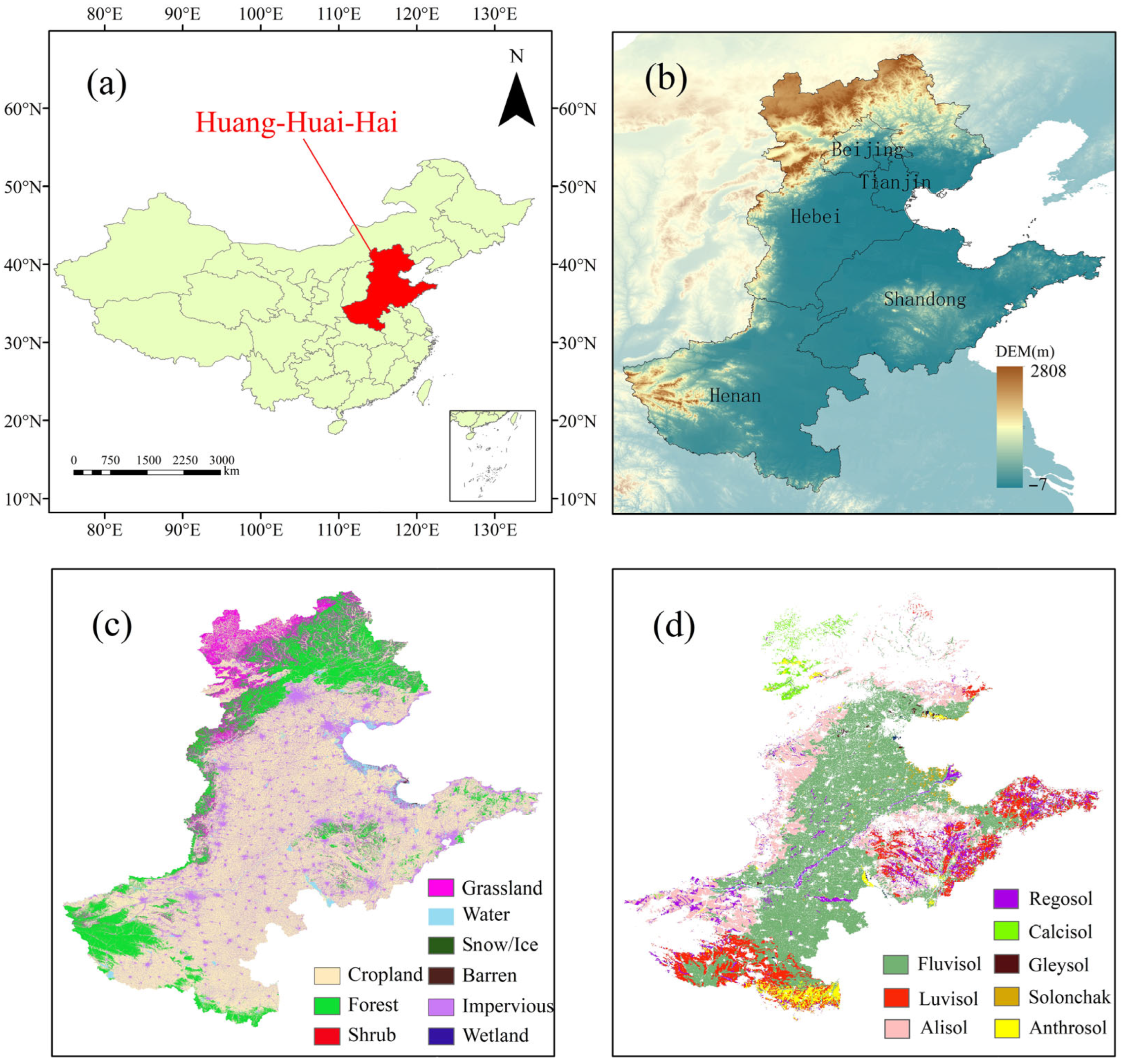
Figure 1. Overview of the study area: (ad) are the location, the topography, the land cover type, and the cropland soil type, respectively.
Remotesensing 17 03765 g001
Figure 2. Number of in situ soil temperature measurements from stations used in the study.
Remotesensing 17 03765 g002
Figure 3. Monthly model prediction performance at different soil depths. (ae) represent the Mean_R2, Mean_RMSE, Mean_MAE, Mean_NSE, and Mean_Bias, respectively.
Remotesensing 17 03765 g003
Figure 4. Feature importance of 0–5 cm. (a) is the detailed distribution of each variable. (b) is the distribution of variables aggregated into three major categories. Column stacked charts of different colors represent the importance of different variables.
Remotesensing 17 03765 g004
Figure 5. Feature importance of 5–15 cm. (a) is the detailed distribution of each variable. (b) is the distribution of variables aggregated into three major categories. Column stacked charts of different colors represent the importance of different variables.
Remotesensing 17 03765 g005
Figure 6. Spatial distribution of the 18-year average soil temperature. (a,b) show the spatial distribution of the 18-year average soil temperature at 0–5 cm and 5–15 cm depths, respectively. (c,d) show the relationships of soil temperature at 0–5 cm and 5–15 cm depths with latitude and elevation, respectively.
Remotesensing 17 03765 g006
Figure 7. Changes in the overall annual mean temperatures for different soil layers in the study area.
Remotesensing 17 03765 g007
Figure 8. Spatial distribution of temperature trends. (ac) show the Sen’s slope, MK test, and temperature trend comparison across four soil types for the 0–5 cm layer, respectively; subplots (df) mirror (ac) but for the 5–15 cm layer.
Remotesensing 17 03765 g008
Figure 9. Spatial distribution of variability. (a,b) show CV and comparison across four soil types for the 0–5 cm layer, respectively; (c,d) show the same for the 5–15 cm layer. (e,f) show the CV difference between the two soil layers and comparison across four soil types, respectively.
Remotesensing 17 03765 g009
Figure 10. Monthly temperature anomalies in the study area for 0–5 cm (a) and 5–15 cm (b), respectively.
Remotesensing 17 03765 g010
Figure 11. Temperature anomaly variation trends for 0–5 cm across the four seasons. The first row (ad) shows Sen’s slope, and the second row (eh) presents the MK test, arranged from left to right as spring, summer, autumn, and winter. (i) shows the distribution of temperature anomaly trends among four soil types for spring and summer, respectively.
Remotesensing 17 03765 g011
Figure 12. Temperature anomaly variation trends for 5–15 cm across the four seasons. The first row (ad) shows Sen’s slope, and the second row (eh) presents the MK test, arranged from left to right as spring, summer, autumn, and winter. (i) shows the distribution of temperature anomaly trends among four soil types for spring and summer, respectively.
Remotesensing 17 03765 g012
Figure 13. Seasonality variations in the study area.
Remotesensing 17 03765 g013
Figure 14. Spatial distribution of seasonality. In the first four rows, the first column represents data for 0–5 cm, and the second column represents data for 5–15 cm. (a,b) are mean temperatures. (c,d) are regions with positive Sen’s slopes. (e,f) are MK test. (g) compares four soil types for the 0–5 cm and 5–15 cm soil layers.
Remotesensing 17 03765 g014
Figure 15. Correlation and lag between the two soil layers. (a,b) represent the monthly temperature variations in the two soil layers in the region and the relationship between the correlation of the two soil layers and lag time, respectively.
Remotesensing 17 03765 g015
Figure 16. Spatial distribution of the temperature difference trend between 0–5 cm and 5–15 cm soil layers. (a,b) represent Sen’s slope and the MK test, respectively. (c) showing the temperature trend difference between two soil layers across different soil types.
Remotesensing 17 03765 g016
Table 1. Details on predictor variables.
AttributeVariableVariation
Characteristics
Temporal ResolutionSpatial ResolutionSource
Environmental variablesland surface temperature (LST)dynamicallymonthly1 kmZenodo [33]
evapotranspiration (ET)dynamicallymonthly1 kmGoogle Earth Engine [34,35]
normalized difference vegetation index (NDVI)dynamicallymonthly1 kmGoogle Earth Engine [36]
radiation
(Reflectance_1
Reflectance_2
Reflectance_3
Reflectance_4
Reflectance_5
Reflectance_6
Reflectance_7)
dynamicallymonthly1 kmGoogle Earth Engine [37]
Soil propertiessoil moisture (SM)dynamicallymonthly1 kmTibetan Plateau Data Center [38]
Bulk densitystatically 250 mSoilGrids [39]
Sandstatically 250 mSoilGrids [39]
soil organic carbon (SOC)statically 250 mSoilGrids [39]
soil pH (pH)statically 250 mSoilGrids [39]
Topographic factorselevationstatically 1 kmEarthEnv Topography [40]
slopestatically 1 kmEarthEnv Topography [40]
roughnessstatically 1 kmEarthEnv Topography [40]
terrain ruggedness index (tri)statically 1 kmEarthEnv Topography [40]
Disclaimer/Publisher’s Note: The statements, opinions and data contained in all publications are solely those of the individual author(s) and contributor(s) and not of MDPI and/or the editor(s). MDPI and/or the editor(s) disclaim responsibility for any injury to people or property resulting from any ideas, methods, instructions or products referred to in the content.