Dual-Branch Hyperspectral Open-Set Classification with Reconstruction–Prototype Fusion for Satellite IoT Perception

Highlights

What are the main findings?

• The dual-branch network architecture integrating reconstruction and prototype classification effectively enhances feature discriminability and improves the detection rate of unknown classes.
• The decision framework based on the fusion strategy of prototype distance and reconstruction error significantly enhances the robustness of the model in open-set scenarios.

What is the implication of the main finding?

• The proposed dual-branch architecture provides a viable solution for satellite Internet of Things to handle high-dimensional data and detect unknown terrain features.
• The established fusion strategy mechanism significantly enhances the practicality and reliability of remote sensing systems in open environments.

Abstract

The satellite Internet of Things (SatIoT) enables real-time acquisition and large-scale coverage of hyperspectral imagery, providing essential data support for decision-making in domains such as geological exploration, environmental monitoring, and urban management. Hyperspectral remote sensing classification constitutes a critical component of intelligent applications driven by the SatIoT, yet it faces two major challenges: the massive data volume imposes heavy storage and processing burdens on conventional satellite systems, while dimensionality reduction often compromises classification accuracy; furthermore, mainstream neural network models are constrained by insufficient labeled data and spectral shifts, frequently leading to misclassification of unknown categories and degradation of cross-regional performance. To address these issues, this study proposes an open-set hyperspectral classification method with dual branches of reconstruction and prototype-based classification. Specifically, we build upon an autoencoder. We design a spectral–spatial attention module and an information residual connection module. These modules accurately capture spectral–spatial features. This improves the reconstruction accuracy of known classes. It also adapts to the high-dimensional characteristics of satellite data. Prototype representations of unknown classes are constructed by incorporating classification confidence, enabling effective separation in the feature space and targeted recognition of unknown categories in complex scenarios. By jointly leveraging prototype distance and reconstruction error, the proposed method achieves synergistic improvement in both accurate classification of known classes and reliable detection of unknown ones. Comparative experiments and visualization analyses on three publicly available datasets: Salinas-A, PaviaU, and Dioni-demonstrate that the proposed approach significantly outperforms baseline methods such as MDL4OW and IADMRN in terms of unknown detection rate (UDR), open-set overall accuracy (OpenOA), and open-set F1 score, while on the Salinas-A dataset, the performance gap between closed-set and open-set classification is as small as 1.82%, highlighting superior robustness.

1. Introduction

The Satellite Internet of Things (SatIoT) represents a deep integration of satellite communication and IoT technologies, enabling global information exchange and communication between objects and between humans and objects [1]. The rapid development of SatIoT has broken down the traditional barriers in the “acquisition-transmission-analysis” chain of hyperspectral remote sensing data, achieving real-time collection and wide-area coverage of hyperspectral images. This provides crucial data support for refined decision-making in fields such as geological exploration, environmental monitoring, and urban management [2,3,4]. As an important branch of remote sensing technology, hyperspectral remote sensing serves as a key enabler for precise perception in SatIoT systems [5]. Open-set recognition, as a critical methodological approach, operates by modeling only a subset of known terrain categories during training, while simultaneously achieving accurate identification of these known categories and effective detection of unknown categories in practical applications [6]. This capability is of paramount importance for enhancing the practicality and reliability of satellite remote sensing systems in open environments. As shown in Figure 1, the workflow of SatIoT primarily consists of front-end and back-end components. The front-end, implemented through edge computing units onboard satellites, is responsible for in-orbit data acquisition and lightweight data value extraction.

The processed information is then transmitted to ground-based back-end servers, which undertake the core Open-set classification task to achieve final terrain classification. However, in practical applications of SatIoT hyperspectral data, the dual challenge of achieving efficient and accurate classification of known terrain categories while reliably detecting unknown categories remains a critical unresolved problem. The hyperspectral open-set classification method proposed in this paper is developed specifically to address this challenge.

Modern hyperspectral imaging systems have achieved breakthroughs in spatial resolution at the decimeter level, enabling the acquired imagery to precisely characterize differences in physical structures and chemical properties of ground objects [7], thereby establishing a robust data foundation for pixel-wise terrain classification. As a core link in the SatIoT-driven intelligent applications, hyperspectral remote sensing classification directly determines the efficiency and reliability of converting spectral data into decision-making value, and its goal is to uniquely assign each pixel in the image to a corresponding land cover type and assign a category label [8]. However, the classification task in the SatIoT scenario faces two challenges: on the one hand, the high-dimensional characteristic of hyperspectral data—each pixel containing hundreds of spectral dimensions—leads to a surge in data volume, which is difficult for the storage and processing capabilities of traditional satellite systems to bear. Conventional linear dimensionality reduction methods tend to lose key features when alleviating this pressure, while manually designed feature extraction templates are limited by expert experience, further restricting the improvement of classification performance [9]. On the other hand, although neural networks can automatically mine the inherent laws of data and have become the current mainstream classification technology, they are affected by the complexity of SatIoT application scenarios and face two core challenges—annotated samples are difficult to cover all ground object categories under wide-area coverage, and when the model encounters unknown categories not included in the training set, it is easy to misclassify them as known categories, resulting in a sharp drop in accuracy [10]. In addition, ground objects in different regions have significant spectral heterogeneity, and the model performance is prone to degradation in cross-regional applications, which seriously hinders the reliable implementation of SatIoT.

To address the aforementioned challenges, open-set hyperspectral classification introduces a mechanism of “known class discrimination + unknown class detection” [6], with existing methods generally divided into two categories: generative model-based and discriminative model-based approaches [11]. Generative model-based methods mostly rely on deep generative models such as GANs and introduce unknown class information to improve classification performance by synthesizing samples with distributions different from those of known classes. OpenGAN [12] employs metric learning to generate approximate samples yet remains largely constrained to distributions similar to those of known classes. Subsequent studies [13,14,15,16] have enhanced sample quality by incorporating attention mechanisms or feature constraints, reducing the distributional gap with real unknown classes. However, such approaches still face two major challenges: first, the generated samples depend heavily on strong prior assumptions, making it difficult to cover the true distribution of unknown classes; second, the high-dimensional correlations inherent in hyperspectral data substantially increase the complexity of sample generation and computational cost. Discriminative model approaches directly learn the distribution of known classes and construct decision boundaries. Liu et al. [17] were the first to introduce the concept of open-set classification into the hyperspectral domain by adding an Openmax layer to a 3D convolutional network, which alleviated overconfident predictions but struggled with complex data distributions. Subsequent works [18,19,20,21] improved feature discriminability through prototype constraints, reciprocal point learning, or reconstruction mechanisms, which enhanced unknown class detection to some extent but remained limited by class imbalance, insufficient reconstruction, or boundary distortion. More recent work [22] combined a variational autoencoder (VAE) to generate pseudo-known samples and identified unknown classes via feature distance, achieving favorable performance in closed-set classification but exhibiting high dependency on the quality of training samples. Overall, although discriminative models avoid the computational overhead of generation, their decision boundaries are easily perturbed in noisy scenarios, leading to higher false detection rates.

Furthermore, based on the proposed methodology, this paper constructs an efficient processing architecture comprising “front-end-satellite edge-side data cleaning” and “back-end-cloud server networked algorithm classification”. When processing hyperspectral images at the satellite front-end, preprocessing is first performed to eliminate errors in the raw data. Initially, radiometric calibration is conducted: the built-in calibration coefficients of the satellite payload are invoked to convert the Digital Number (DN) values output by the sensor into radiance values, thereby addressing the issue of inconsistent sensor responses. Subsequently, atmospheric correction is implemented, integrating real-time atmospheric parameters (such as aerosol concentration and water vapor content) and leveraging the MODTRAN model to eliminate interferences from atmospheric scattering and absorption, thus restoring the true spectra of ground features. Concurrently, geometric precision correction is carried out: based on satellite orbit data and ground control points, geometric distortions caused by the Earth’s curvature and attitude variations are corrected to ensure the accuracy of the image’s geographic coordinates. The data cleaning phase focuses on optimizing the preprocessed data. Anomalies in spectral curves, such as jump points and saturation values, are identified through statistical analysis and repaired using adjacent pixel interpolation. For isolated noise induced by sensor dark current and cosmic rays, smoothing is performed using median filtering and mean filtering. Meanwhile, based on the signal-to-noise ratio of each band, edge bands with low information content are discarded, while effective bands are retained.

The combined computational load of the adopted simplified MODTRAN model and the lightweight PCA algorithm amounts to approximately one-fifth of that required by conventional algorithms. To enhance the downlink efficiency, a “real-time quality screening” step has been incorporated into the satellite-side data preprocessing pipeline. Specifically, after imagery is corrected via MODTRAN/PCA, a rapid spectral-threshold-based detection algorithm is applied to automatically calculate cloud coverage. This ensures that only high-quality images with cloud coverage ≤ 10% are selected for downlinking, while effectively filtering out invalid data.

Ultimately, a high-quality dataset to be processed is generated. The data acquired at the satellite edge-side undergoes confidentiality processing and vectorization, providing reliable support for subsequent open-set classification algorithms for hyperspectral images. To this end, this study proposes an integrated solution for open-set hyperspectral classification that augments known class classification with additional detection of unknown categories, thereby effectively preventing the network from misclassifying unknown samples as belonging to a known class [23].

The main contributions of this study are as follows:

• A fusion strategy-based recognition mechanism is proposed. By jointly utilizing two complementary criteria, namely “reconstruction error” and “prototype distance”, this mechanism effectively discriminates between known and unknown classes, thereby enhancing the robustness and performance of open-set classification.
• A targeted feature optimization method is designed. Through the spatial–spectral attention module and confidence-based construction of unknown-class prototypes, the spatial–spectral characteristics of hyperspectral data are fully exploited, achieving clear separation between known and unknown classes at the feature level.
• Experiments conducted on three publicly available datasets, together with ablation analyses against multiple state-of-the-art methods, demonstrate that the proposed model achieves superior performance in hyperspectral open-set classification, not only outperforming competing approaches in terms of UDR, OpenOA, and open-set F1 score, but also maintaining a low accuracy gap between closed-set and open-set scenarios, thereby exhibiting enhanced robustness.

2. Related Works

Early deep learning-based hyperspectral remote sensing image classification was conducted in a closed-set environment. However, due to its limitations in practical applications, the open-set classification method was proposed. To evaluate the performance of open-set classification, relevant evaluation metrics for open-set classification models have been put forward.

2.1. Methods Related to Satellite Hyperspectral Data Preprocessing

In the field of hyperspectral image classification, to address the issue that traditional Attribute Profiles (APs) can only handle single-level features and struggle to fully exploit multi-dimensional spatial information, Extended Attribute Profiles ($EAPs$) [5] are often adopted as a preferred solution. The core of $EAP$ lies in the multi-scale and multi-dimensional extension of attribute profiles, enabling more comprehensive extraction of spatial features from hyperspectral images and providing richer feature support for subsequent classification tasks. In terms of the construction process, the generation of $EAP$ involves several key steps. Firstly, Principal Component Analysis (PCA) is performed for dimensionality reduction on the original Hyperspectral Image (HSI) data. This is because hyperspectral data is characterized by high dimensionality and redundant information; PCA can retain approximately 99% of the total variance in the data and select the top m most representative Principal Components (PCs), which not only reduces data complexity but also decreases the computational load of subsequent processing. Secondly, for each selected principal component, an AP is constructed individually. By utilizing morphological attribute filters (based on attributes such as area and standard deviation) and combining them with a set of thresholds, filtering operations such as thickening and thinning are applied to the connected regions of the principal-component images, resulting in the AP corresponding to each principal component. The thresholds can be determined through manual trial-and-error or automatic algorithms (e.g., methods based on attribute value statistics) to adapt to different data characteristics. Finally, the APs corresponding to all principal components are stacked and integrated, with redundant information in the original principal components (such as duplicate basic feature layers) removed, forming the final $EAP$ Its mathematical expression is as follows:

$$EAP\left(g\right)=\{AP\left(g_1\right), AP\left(g_2\right),\dots , AP\left(g_m\right)\}$$

(1)

In the formula, $g_1$, $g_2$, …, $g_m$ represent the first m principal components of hyperspectral data after PCA transformation, and $AP\left(g_i\right)$ denotes the attribute profile corresponding to the i-th principal component. $EAP$ possesses the dual advantages of multi-scale and multi-dimensional fusion. The multi-scale characteristic is reflected in its ability to capture spatial features of connected regions with different sizes in hyperspectral images by setting different attribute thresholds—for instance, small thresholds can extract detailed texture information, while large thresholds can reflect macro regional distribution. The multi-dimensional characteristic originates from its integration of multiple principal components: each principal component focuses on reflecting different spectral features of hyperspectral data, and the corresponding AP can extract spatial information under different spectral dimensions. $EAP$ realizes the fusion of this information through stacking, which effectively alleviates the problems of “same spectrum with different objects” and “same object with different spectra” in hyperspectral images. In terms of satellite edge-side data cleaning, $EAP$ serves as a key link connecting hyperspectral data preprocessing and deep classification models. For example, in the AP-SAE model, the spatial features extracted by $EAP$ are combined with the spectral features extracted by the Stacked Autoencoder (SAE) to form spectral–spatial fusion features. Here, the optimization effect of $EAP$ on classification performance is more prominent, providing important technical support for applications such as large-scale land cover monitoring in satellite Internet of Things systems.

2.2. The Principle of Closed-Set Classification Based on Deep Learning

Neural networks have been widely applied in hyperspectral remote sensing images due to their efficient feature extraction capability. A classical neural network model for closed-set classification of hyperspectral data typically consists of a convolutional neural network (CNN)-based feature extractor and a multi-layer perceptron (MLP)-based multiclass classifier. Specifically, the CNN first extracts features from the input samples, and then the MLP projects these features into a multidimensional vector, where each dimension corresponds to a probability score representing the likelihood that the sample belongs to a particular class. Finally, the class associated with the maximum probability score is selected as the label, thereby completing the classification process [24].

However, when applying a trained model to real-world scenarios, it inevitably encounters categories that are absent from the training set, while the model can only assign such unknown samples to one of the existing classes. Therefore, open-set classification is required, which adds the identification of unknown classes on the basis of known-class classification and assigns a separate label to classes not present in the training set [25].

2.3. Classical Methods for Hyperspectral Open-Set Classification

Existing open-set classification methods are categorized into generative model-based methods and discriminative model-based methods [26]. Among them, generative model-based methods use generative networks to synthesize unknown-class samples that are as different from known classes as possible. These samples are merged with known-class samples to train a multi-class classifier, which simultaneously classifies both known and unknown classes in the target domain [27]. However, these methods usually treat all unknown classes in the test set as a single category, ignoring their diversity and complexity, and most generative models struggle to simulate real unknown classes. Discriminative model-based methods analyze the sample features or losses in the training set, select abnormal samples that do not conform to the model’s fitting function as potential unknown classes, and determine the decision threshold for unknown classes accordingly. They achieve open-set classification by combining this threshold with a classifier. The underlying principle is that the training process of a neural network involves the model performing backpropagation iterations based on sample features or labels to fit the functional relationship between samples and labels, thereby minimizing the loss.

2.4. Evaluation Metrics for Open-Set Classification

This section introduces the relevant evaluation metrics for open-set classification models, including the Openness metric, Closed Overall Accuracy (ClosedOA), Open Overall Accuracy (OpenOA), Unknown Detect Rate (UDR), and classification F1-score, to facilitate the evaluation of model performance in subsequent experiments.

To measure the openness of open-set classification tasks, Geng et al. [6] defined an openness metric based on the proportion of the number of known classes to unknown classes. The definition formula is as follows:

$$Openness=1-\sqrt{{\displaystyle \frac{2\times W}{2\times W+Q}}}$$

(2)

Herein, W represents the number of known classes in the training data, and Q denotes the number of actual unknown classes.

It is used to measure the model’s ability to detect unknown-class samples [28], and its calculation formula is as follows:

$$\mathrm{UDR}={\displaystyle \frac{n_{right}^{Unk}}{n_{total}^{Unk}}}$$

(3)

Herein, $n_{right}^{Unk}$ represents the number of unknown classes correctly identified, and $n_{total}^{Unk}$ denotes the total number of unknown classes.

ClosedOA is used to measure the closed-set performance of the model during testing, and its calculation formula is as follows:

$$\mathrm{ClosedOA}={\displaystyle \frac{{\displaystyle \sum _{w=1}^W{n}_{right}^w}}{{\displaystyle \sum _{w=1}^W{n}_{total}^w}}}$$

(4)

OpenOA is used to measure the overall performance of the model during testing [29], and its calculation formula is as follows:

$$\mathrm{OpenOA}={\displaystyle \frac{n_{right}}{n_{total}}}$$

(5)

Herein, $n_{right}$ represents the number of correctly classified samples, and $n_{total}$ denotes the total number of samples.

3. Proposed Method

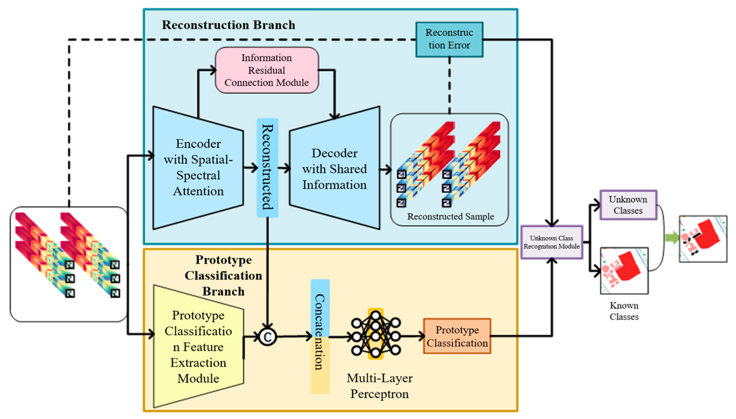
The open-set classification framework we proposed, as illustrated in Figure 2, consists of a dual-branch structure comprising a reconstruction branch and a prototype classification branch. The reconstruction branch generates samples and calculates errors, while the prototype classification branch extracts features and performs classification. Subsequently, the unknown class identification module combines the results of the two branches to achieve hyperspectral open-set classification.

3.1. Hyperspectral Open-Set Classification Algorithm Framework Combining Reconstruction and Prototype

Building upon the original autoencoder for multi-task learning of reconstruction and classification [24], our method constructs two CNN branches based on the two tasks of reconstruction and prototype classification, respectively. The training set is fed into both branches simultaneously for feature extraction. Meanwhile, inspired by Han et al. [30], we concatenate the features from the reconstruction network and the classification network. This allows the network to acquire richer information for subsequent classification. The algorithm flow is depicted in Figure 2. We summarize the pseudocode for the Open-Set Hyperspectral Image Classification Framework in Algorithm 1.

Algorithm 1 Open-Set Hyperspectral Image Classification Framework (Corresponding to Figure 2)
Require: HSI: Hyperspectral Image (raw spatial-spectral data, 3D cube [height × width × spectral bands]), 1: Prototype_Params: Prototype classification hyperparameters (e.g., prototype count = 20, feature dim = 64, distance metric = Euclidean), 2: Recon_Params: Reconstruction branch hyperparameters (e.g., attention layers = 2, residual weight = 0.3, loss type = MSE) Ensure: Class_Map: Pixel-wise classification map (labels: known classes [1..K], unknown   class [0]) 3: Initialize reconstruction branch: encoder (spatial-spectral attention), residual module, decoder (shared info) with Recon_Params 4: Initialize prototype branch: feature extractor (3 convolutional layers), MLP (2 hidden layers) with Prototype_Params 5: for each pixel p in HSI do 6: Extract spectral vector Sp ∈ ℝspectral bands from pixel p
▷ Reconstruction branch: enhance and reconstruct spectral features
7: Attended_Featsp = Attention Encoder(Sp)	▷ Weight critical spatial-spectral components
8: Enhanced_Featsp = Residual Connection(Attended_Featsp, Sp)	▷ Preserve fine-grained information
9: Reconstructed_Sp = Shared Info Decoder(Enhanced_Featsp)	▷ Reconstruct input spectral vector
10: Recon_Errorp = ∥Sp − Reconstructed_Sp∥2	▷ L2-norm reconstruction error
▷ Prototype classification branch: fuse and classify
11: Proto_Featsp = Feature Extractor(Sp)	▷ Extract high-level semantic features
12: Fused_Featsp = [Proto_Featsp; Recon_Errorp]	▷ Concatenate dual-modal features
13: Known_Scoresp = MLP(Fused_Featsp)	▷ Output scores for K known classes
▷ Unknown class recognition via confidence thresholding
14: Max_Confidencep = max(Known_Scoresp)	▷ Highest confidence of known classes
15: if Max_Con f idencep < 0.5 then	▷ Threshold from Prototype_Params
16: Labelp = 0	▷ Mark as unknown class
17: else
18: Labelp = arg max(Known_Scoresp)	▷ Assign to most confident known class
19: end if
20: Class_Map(p) ← Labelp	▷ Update classification map
21: end forreturn Class_Map

In the reconstruction branch, the model compresses the input samples into intermediate vectors via an encoder. The decoder decodes the intermediate vectors by combining information from residual connection modules and calculates the error between the input samples and the decoder output as the reconstruction loss. This loss constrains the encoder–decoder to compress and then fully reconstruct the known classes.

In the prototype classification branch, sample features are first extracted, followed by concatenating the classification features with the intermediate vectors. The concatenated features are input into a MLP for feature fusion. The distance between the fused features and class prototypes is calculated for classification. Then, unknown class prototypes are constructed based on classification confidence, and a contrastive loss is built according to the distance between class prototypes and features. This loss constrains the inter-class features to be far apart.

Since unknown classes do not participate in the training of the reconstruction branch, their reconstruction errors are much larger than those of known classes. Additionally, the prototype classification branch constrains the known class features to be far from the unknown class prototypes through contrastive loss. During testing, samples with high reconstruction errors and small distances to unknown class prototypes are identified as unknown classes.

The unknown class recognition module counts the reconstruction errors and distances to unknown class prototypes of all samples in the training set and automatically determines the unknown class discrimination boundary through function fitting based on distribution characteristics.

3.2. Reconstruction Branch with Attention Interaction

The network architecture of the reconstruction branch consists of two parts: an encoder and a decoder. The encoder comprises two encoding blocks, a Global Average Pooling (GAP) layer, and a Fully Connected (FC) layer. The two encoding blocks perform forward propagation and backward iteration through residual connections, and finally, after passing through the GAP and FC layers, an intermediate vector for both reconstruction and classification tasks is obtained. This structure enables the encoder to extract high-level semantic information while retaining important low-level feature information.

Each encoding block consists of a Batch Normalization (BN) layer, a Rectified Linear Unit (ReLU) layer, a 2D Convolutional (Conv2D) layer, and a Spectral Spatial Attention (SSA) layer. Figure 3 illustrates the process by which the encoder compresses input samples into intermediate vectors.

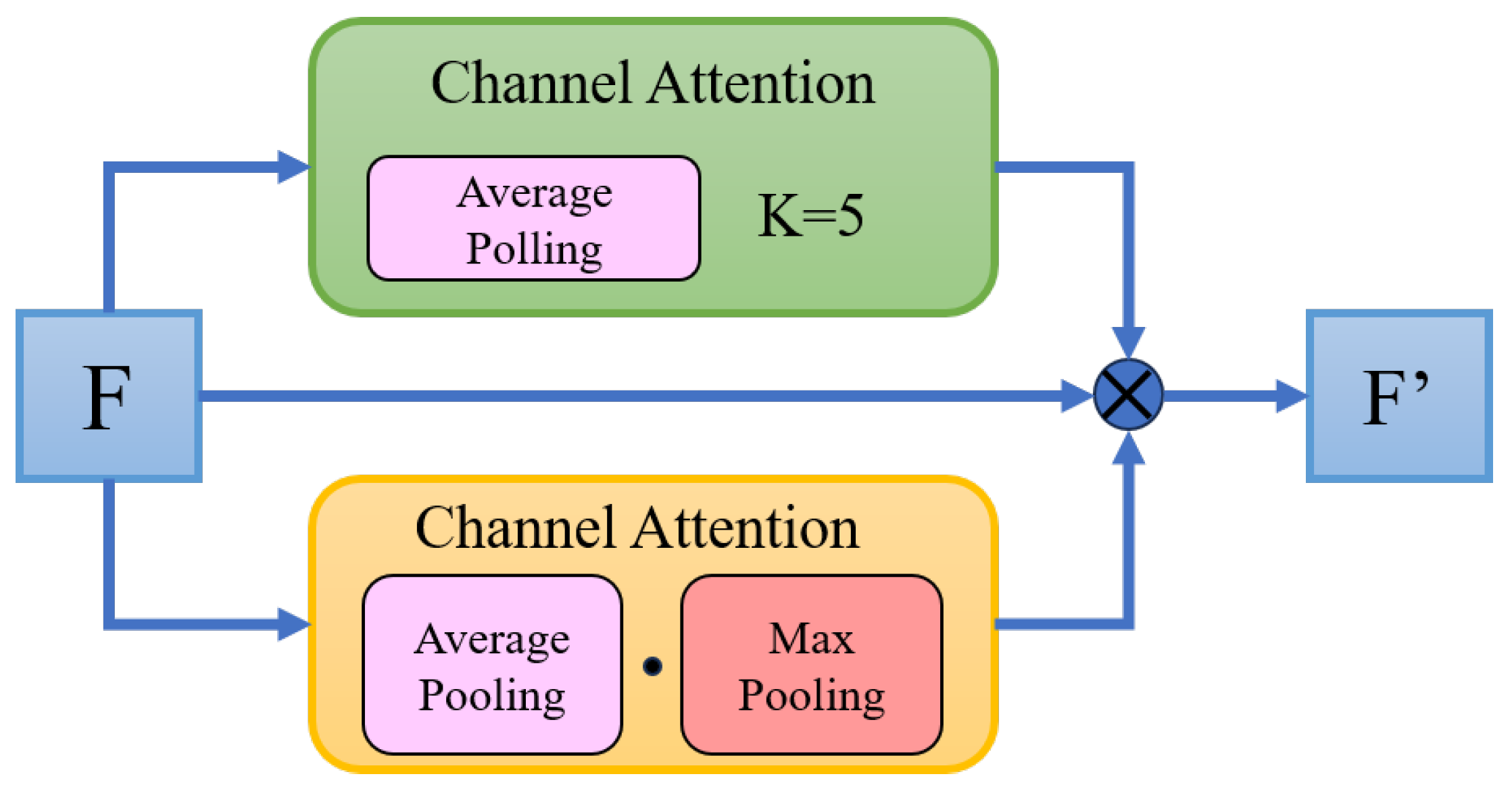
According to the characteristics of hyperspectral data, the SSA layer modifies the serial structure of the original Convolutional Block Attention Module (CBAM) into a parallel structure, calculates channel attention and spatial attention simultaneously, and couples them through multiplication, enabling the network to adapt to the spectral–spatial joint features in hyperspectral images, as illustrated in Figure 4 For the Channel Attention Mechanism (CAM), after performing GAP on the original features, multi-kernel 1D convolution is adopted for local feature extraction, which retains the correlation between channels while capturing positions with important information; for the Spatial Attention Mechanism (SAM), it first uses Global Max Pooling (GMP) and GAP on each channel of the input features to aggregate channel information, obtaining two 2D features containing only spatial information, then concatenates these two features, fuses them via a 2D convolution kernel, and finally passes them through an activation layer to generate the weight coefficients of spatial attention. The channel attention, spatial attention, and input feature map are multiplied to generate the final feature map, and the SSA layer can focus on key features in both the channel and spatial dimensions of hyperspectral images while suppressing irrelevant noise and redundant information, thereby helping the encoding block to capture the key features of hyperspectral data more efficiently.

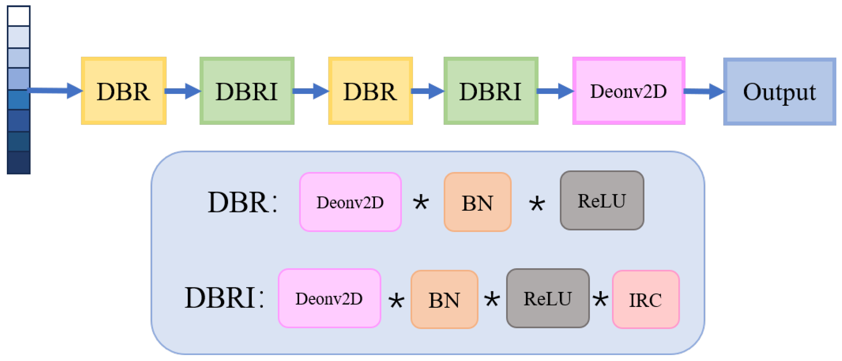
In addition, each encoding block transmits the acquired spectral–spatial features to the decoder through an Information Residual Connection (IRC) module, enabling the decoder to improve reconstruction performance. The structure of the decoder is shown in Figure 5. It consists of 4 decoding blocks, each containing a 2D Deconvolutional (Deconv2D) layer, a BN layer, a ReLU layer, and an IRC module. Based on the features decoded by the previous layer and combined with the information from the encoder of the same depth carried by the IRC module, each decoding block reconstructs the features back to the original input samples. Figure 5 illustrates the process by which the decoder reconstructs the intermediate vectors.

During the encoding process, pooling and convolution operations in neural networks may cause the loss of low-level information, making it difficult for the information carried by intermediate vectors to realize the reconstruction of hyperspectral patches. To address this issue, this paper utilizes the IRC module, taking the features extracted by the encoder as auxiliary information for the decoder’s reconstruction. Meanwhile, to prevent the decoder from directly using the low-level features of the encoder for reconstruction, which would affect the encoder’s effective compression of intermediate vectors, this paper chooses to fuse the features of the encoder and decoder at the same depth through addition. Considering that different spectral bands of pixels contain varying degrees of noise, low-level encoded features of different spectral bands thus have different information contents: for cleaner spectral bands, retaining more low-level features helps preserve details; for spectral bands with more noise, a higher proportion of high-level features is required for effective sample reconstruction, thereby improving the overall reconstruction performance of known classes. Therefore, if the same weight is applied to the shallow features from the encoder and the reconstructed features from the decoder, additional noise may be introduced, causing the model to mistakenly treat noise as part of known classes and reducing its sensitivity to anomalies (unknown classes). The network structure of the IRC module is illustrated in Figure 6.

Through the IRC layer, the decoding blocks can share features of the same depth from the encoder and achieve forward propagation and backward iteration via concatenation. Constrained by the reconstruction loss, the model can learn the common features of known classes, improve the overall reconstruction performance of known classes, and realize the complete reconstruction of known classes. However, the feature distribution of unknown classes differs from that of known classes, and the model fails to capture the features usable for reconstruction. As a result, the reconstruction performance of unknown classes is far worse than that of known classes, so known classes and unknown classes can be distinguished by their reconstruction performance.

3.3. Contrastive Prototype Classification Branch with Confidence Integration

The contrastive prototype classification branch consists of a feature extractor and a confidence-aware contrastive prototype classification module, where the structure of the feature extractor is identical to that of the encoder in the reconstruction branch. After obtaining the feature $f_{pro}$, it is concatenated with $f_{rec}$ from the reconstruction module and fed into a MLP for dimensionality reduction.

$$f=\mathrm{MLP}([f_{pro};f_{rec}])$$

(6)

The contrastive prototype classification module achieves classification by calculating the distance between features and each class prototype, where the class prototypes include W known-class prototypes and 1 unknown-class prototype, denoted as $\overrightarrow{P}=\{P^1,P^2,\dots ,P^w,\dots ,P^W\}$. The known-class prototypes exist in the form of network parameters: they are randomly initialized during definition, and their positions are updated through backward iteration by the optimizer based on subsequent classification and contrastive losses. The unknown-class prototype is calculated as the mean value of samples with low confidence.

The original prototype-based classification is implemented using Euclidean distance. Inspired by Gjorgiev et al. [31], Mahalanobis distance utilizes a covariance matrix to eliminate the correlation between different dimensions of features, making it easier to detect anomalous samples during clustering. Since this paper needs to select anomalous samples with low confidence to construct the unknown-class prototype, classification is performed by calculating the Mahalanobis distance between features and prototypes. First, the mean value $\mu$ of all samples in the current iteration is calculated; then, the covariance matrix $S$ is derived based on this $\mu$. The calculation formulas are as follows:

$$S={\displaystyle \frac{1}{Batch\_Size-1}}\sum _{i=1}^{Batch\_Size}(f_i-\mu ){(f_i-\mu )}^T$$

(7)

Then, $S$ is used to calculate the Mahalanobis distance. For the feature $f_i$ of the $i$-th sample and the prototype of the w-th class, the calculation formula of its Mahalanobis distance $d(f_i,P^w)$ is as follows:

$$d(f_i,P^w)=\sqrt{{(f_i-P^w)}^T{S}^{-1}(f_i-P^w)}$$

(8)

Finally, the probability that the i-th sample belongs to the w-th class is calculated based on the Mahalanobis distance:

$$\widehat{p_i^w}={\displaystyle \frac{e^{-d(f_i,P^w)}}{{\displaystyle \sum ^{\underset{N}{j=1}}}{e}^{-d(f_i,P^j)}}}$$

(9)

After obtaining all probabilities for the W classes, the label w corresponding to the maximum probability $\widehat{p_i^w}$ is elected as the classification result.

$$y_i=\mathit{argmax}(\left\{\widehat{p_i^w}\right\})$$

(10)

After completing the classification, the information entropy is calculated based on the currently obtained $\widehat{p_i^w}$ to determine the confidence level of the sample:

$${\mathit{Confidence}}_i=1+{\displaystyle \frac{{\sum }_{w=1}^W\left(\widehat{p_i^w}\mathit{log}\left(\widehat{p_i^w}\right)\right)}{\mathit{log}(W)}}$$

(11)

where W is the total number of classes, and $\log (W)$ is a normalization factor that ensures the entropy ranges between $[0,1]$. When the entropy is 0, the confidence level is 1, indicating that the model is completely certain. When the entropy is $\log (W)$, the confidence level is 0, meaning the model is completely uncertain about which class the sample belongs to, and such a sample is regarded as an anomalous sample. As the model iterates and optimizes, the confidence level of known classes increases accordingly, while the confidence level of anomalous samples remains relatively low. By employing a deep learning parameter search network combined with empirical analysis, we ultimately select the bottom 10% of samples with the lowest confidence as anomalous specimens. The prototype for unknown classes is then computed as the mean representation of these selected anomalous samples:

$$P^{W+1}={\displaystyle \frac{1}{n_w}}{\displaystyle \sum _{i=1}^{n_w}{f}_i}$$

(12)

After obtaining the prototypes of known classes and the unknown class, the Prototype Contrastive Loss (PCL) is calculated based on the sample features and prototypes:

$$L_{\mathrm{con}}={\displaystyle \frac{1}{N}}{\displaystyle \sum _{i=1}^N\left[d(f_i,P^{y_i})+{\displaystyle \sum _{w\ne y_i}\max (0,m-d(f_i,P^w))}\right]}$$

(13)

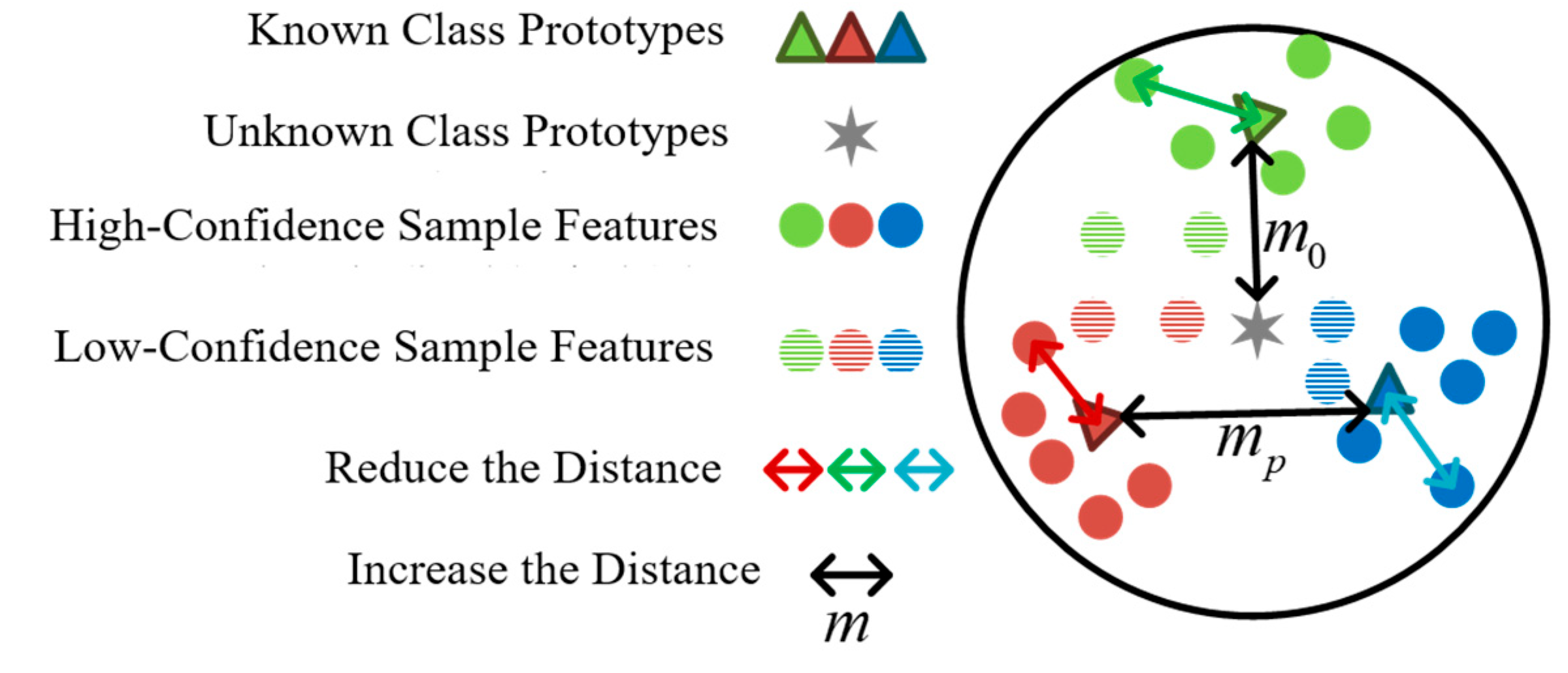
where $m$ is the margin distance, which is used to control the distance of negative sample pairs. The model optimizes feature representations and class prototypes through the PCL, thereby enhancing intra-class compactness and inter-class separability, and its implementation effect is illustrated in Figure 7. Colored arrows represent samples with the same label as the class prototype, which are expected to attract each other. Black arrows represent negative samples, which are expected to repel each other. Through contrastive learning, class prototypes are made to be far apart from each other. $m_p$ is the margin distance between known classes, which is set as the maximum distance among all positive sample pairs in the current batch. Considering that the feature space occupied by the unknown class is unknown, to reserve sufficient feature space, the margin distance between known classes and the unknown class is set to 3 times that of $m_p$.

In addition, this paper also calculates the cross-entropy loss for classification:

$$L_{\mathrm{ce}}=-{\displaystyle \frac{1}{Batch\_Size}}{\displaystyle \sum _{i=1}^{Batch\_Size}{\displaystyle \sum _{w=1}^W\left(p_i^w\log \left(\stackrel{\wedge }{p_i^w}\right)\right)}}$$

(14)

where $Batch\_Size$ denotes the number of samples in this iteration, $p_i$ is the one-hot encoded vector of the sample’s true label $y_i$, $p_i^w=\left\{\begin{array}{cc}1& w=y_i\\ 0& w\ne y_i\end{array}\right.$, and $\widehat{p_i^w}$ is the probability that the model predicts sample i belongs to class w.

The weight of the reconstruction loss is set to $\lambda$, and the weight of the prototype contrastive loss is set to $\eta$. The final total loss function is as follows:

$$L_{total}=\lambda L_{rec}+(1-\lambda )(\eta L_{con}+L_{ce})$$

(15)

3.4. Unknown Category Recognition Module

After completing the model training, the model is capable of reconstructing known classes and performing prototype-based classification. Next, to automatically determine the threshold for unknown classes, all samples in the training set are input into the model to recalculate their reconstruction errors and distances from the unknown class prototype. Then, functions are used to fit the distribution of reconstruction errors and the distribution of distances from the unknown class prototype, respectively. Some anomalous samples in the distributions are selected as unknown classes to determine the threshold for subsequent identification of unknown classes.

To observe the characteristic distribution of reconstruction errors across all known classes, a histogram visualization was generated for the reconstruction errors of all training set samples in the Pavia University (PaviaU) dataset, as shown in Figure 8.

It can be observed that the losses of known classes are mainly concentrated in the range of 0 to 5, and the number of samples decreases gradually in a steep manner beyond 5. Larger losses indicate that the deep learning model has not fully optimized these instances; thus, the samples in the tail region should be regarded as unknown classes unseen by the model. Considering that other datasets also exhibit similar distributions, but with different tail decline slopes, to enable the model to automatically determine the threshold, this paper adopts the Generalized Pareto Distribution (GPD) to model the tail distribution.

First, the minimum reconstruction error corresponding to the top 10% of samples with the largest reconstruction errors is calculated as $v_{\min }$. Then, the samples with reconstruction errors higher than $v_{\min }$ are taken as the tail distribution of the known classes. Next, the GPD is used to fit the tail distribution, and its corresponding cumulative distribution function (CDF) can be expressed as follows:

$$G_{\xi ,\mu }(v)=\left\{\begin{array}{cc}1-{\left(1+{\displaystyle \frac{\xi \cdot v}{\mu }}\right)}^{-{\displaystyle \frac{1}{\xi }}},& \xi \ne 0\\ 1-e^{-{\displaystyle \frac{v}{\mu }}},& \xi =0\end{array}\right.$$

(16)

Among them, $\xi$ and $\mu$ are obtained via maximum likelihood estimation (MLE). Then, the top 5% of samples in the tail are selected as candidate unknown classes, i.e., the threshold is determined as $v_o$ that satisfies $G_{\xi ,\mu }(v_o-v_{\min })=1-5\%$, which is calculated by the following formula:

$$v_o=\left\{\begin{array}{cc}{v}_{\min }+{\displaystyle \frac{\mu }{\xi }}\left({\left({\displaystyle \frac{1}{0.05}}\right)}^{\xi }-1\right)& \xi \ne 0\\ v_{\min }-\mu \ln (0.05)& \xi =0\end{array}\right.$$

(17)

After determining the threshold, the rule for identifying unknown classes based on reconstruction errors is as follows:

$$y_i^{rec}=\left\{\begin{array}{cc}Unk& v_i>v_o\\ y_i& v_i<v_o\end{array}\right.$$

(18)

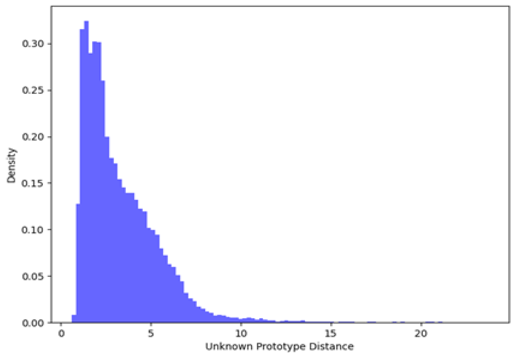
Regarding the prototype distances of unknown classes, the histogram visualization of the prototype distances between all samples in the training set and the unknown class prototypes is shown in Figure 9.

It can be observed that the prototype distances in the training set exhibit a bimodal distribution, where the distribution with larger distances has a higher density and the one with smaller distances has a lower density. During model training, known-class prototypes are constrained to be far from unknown-class prototypes, while known-class samples are constrained to be close to known-class prototypes. Therefore, the distribution with large distances to unknown-class prototypes and high density corresponds to high-confidence known-class samples. In contrast, the distribution with small distances and low density corresponds to low-confidence anomalous samples, which are considered to lie on the boundary between known and unknown classes. In this paper, these samples are classified into the unknown class during partitioning.

To automatically determine the threshold for segmenting anomalous samples and known-class samples, this paper adopts the Otsu threshold segmentation algorithm to identify the optimal segmentation threshold between the two distributions. First, the mean value of all unknown-class distances is calculated as follows:

$$d_{\mu }={\displaystyle \frac{1}{n}}{\displaystyle \sum _{i=1}^n{d}_i}$$

(19)

where $n$ denotes the total number of samples. Next, a threshold $d_t$ is randomly determined, and binary classification of known classes and unknown classes is performed accordingly: samples with a distance greater than $d_t$ are classified into known class $Kn$, while those with a distance smaller than $d_t$ are classified into the unknown class $Unk$. Then, their mean values are calculated separately:

$$\begin{array}{cc}{d}_{\mu \_K\mathrm{n}}={\displaystyle \frac{1}{n_{Kn}}}{\displaystyle \sum _{d_i\in Kn}{d}_i}& d_{\mu \_Unk}={\displaystyle \frac{1}{n_{Unk}}}{\displaystyle \sum _{d_i\in Unk}{d}_i}\end{array}$$

(20)

where $n_{Kn}$ denotes the number of samples classified into the known class, and $n_{Unk}$ denotes the number of samples classified into the unknown class. On this basis, the variances of the known class and the unknown class are calculated as follows:

$$g=h_{Kn}{(d_{\mu \_Kn}-d_{\mu })}^2+h_{Unk}{(d_{\mu \_Unk}-d_{\mu })}^2$$

(21)

where $h_{Kn}={\displaystyle \frac{n_{Kn}}{n}}$ and $h_{Unk}={\displaystyle \frac{n_{Unk}}{n}}$ represent the weights of the known class and the unknown class, respectively. A larger variance indicates a greater difference between the known class and the unknown class, leading to a better separation effect. Based on the above formulas, the threshold $d_t$ is traversed from 0 to $\max (d_i)$, and the $d_t$ corresponding to the maximum variance is found:

$$y_i^{pro}=\left\{\begin{array}{cc}Unk& d_i<d_t\\ y_i& d_i>d_t\end{array}\right.$$

(22)

Through the optimization of model parameters using losses, known-class samples tend to exhibit small reconstruction losses and large distances to unknown classes after being fed into the model. However, due to the diverse features of unknown-class samples, their performances in terms of reconstruction errors and distances to unknown classes vary: they may either have small reconstruction losses but be close to unknown classes or be far from unknown classes but have large reconstruction losses. Therefore, unknown classes are identified using “OR” logic based on $y_i^{rec}$ and $y_i^{pro}$.

$$y_i=\left\{\begin{array}{cc}Unk& y_i^{rec}=Unk|y_i^{pro}=Unk\\ y_i& Othercases\end{array}\right.$$

(23)

4. Experiments and Results

4.1. Experimental Data and Setup

4.1.1. Experimental Setup

All experiments in this paper were conducted in a Linux environment with the following configurations: Intel(R) Xeon(R) Gold 5222 CPU @ 3.80 GHz, GeForce RTX 2080 GPU, CUDA V10.2.89, 125 GB memory, Ubuntu 20.04.2 operating system, Python 3.6.13 programming language, and TensorFlow 1.2.0 deep learning framework.

4.1.2. Experimental Dataset

Three public hyperspectral datasets with distinct spectral and spatial characteristics are employed for the open-set classification experiments in this study, namely Salinas-A, PaviaU, and Dioni.

Since the background in the datasets consists of unlabeled samples, which contain both unknown classes and known classes, they cannot be directly used as unknown classes in the experiments. Referring to the study by Sun et al. [18], some known classes in the datasets are selected as unknown classes, and then samples are randomly chosen from the remaining known classes to form the training set. The class division of the three datasets is shown in

Table 1. Class Distribution and Partitioning of Datasets.

Salinas-A				Pavia University			Dioni
ID	Class Name	ntrain	ntest	Class Name	ntrain	ntest	Class Name	ntrain	ntest
1	weeds_1	156	235	Tree	1225	1839	Urban	504	758
2	weeds_2	537	806	Asphalt	2652	3979	Mine	81	123
3	Lettuce_r4	246	370	Brick	1472	2210	Arable	245	369
4	Lettuce_r5	609	915	Bitumen	532	798	Fruit	60	90
5	Lettuce_r6	270	405	Shadow	378	569	Forest	144	217
6	Unknown (Road)	0	799	Unknown (BareSoil Meadow)	0	9674	Dense Scl	144	217
-							Sparce Scl	2014	3021
-	-	-	-				Sparse Veg	2549	3825
-	-	-	-	-	-	-	RockSand	701	1053
-	-	-	-	-	-	-	Water	196	296
-	-	-	-	-	-	-	Coast	644	968
-	-	-	-	-	-	-	Unknown	0	1768
-	-	-	-	-	-	-	(Olive)

. Each pixel in the datasets is assigned a category label, representing the real object or land cover type corresponding to the pixel. The labels of the entire dataset form a 2D matrix with a size of, $H\times B$ which corresponds to the spatial dimensions of the hyperspectral data with a size of $H\times B\times C$.

These three hyperspectral datasets each have unique features: Salinas-A was captured by AVIRIS in the Salinas Valley, USA, in 1992; of the original 224 spectral bands, 204 are retained after processing, with an image size of 83 × 83 pixels and a spatial resolution of 3.7 m per pixel. Derived from artificially planned farmland, it contains crops such as lettuce and grapes as well as soil, where most spectra correspond to plant leaf reflections, requiring refined spectral processing; PaviaU was acquired by ROSIS over the University of Pavia, Italy; after denoising, 102 bands are retained from the original 115, with an image size of 610 × 715 pixels and a spatial resolution of 1.3 m per pixel. It includes 9 categories of urban features (e.g., roads and buildings), characterized by significant spectral differences between categories but imbalanced sample sizes; Dioni was captured by the EO-1 Hyperion sensor over Sicily, Italy, with 224 spectral bands, an image size of 600 × 600 pixels, and a spatial resolution of 1 m per pixel. Comprising 12 land cover types (e.g., olive trees and vineyards), it features clear spatial details, imposing higher requirements on the algorithm’s spatial feature extraction capability.

4.1.3. Parameter Setting

The proposed method employs spatially disjoint sampling for input patches, augmented to four times the original volume. Experimental results demonstrate that optimal performance metrics are achieved with patch sizes of 9 × 9 for Salinas-A, 11 × 11 for PaviaU, and 11 × 11 for Dioni datasets. Batch sizes are configured as 140, 200, and 180, respectively, to balance training efficiency with classification accuracy. The learning rates $lr$ are empirically determined as 3.0, 5.0, and 1.0 for the three datasets, subsequently reduced to 0.1 during fine-tuning phases, with early stopping implemented to prevent overfitting. In the loss function configuration, the reconstruction loss $\lambda$ weight is set to 0.5 while the contrastive loss $\eta$ weight is maintained at 0.4, effectively balancing feature reconstruction quality with inter-class discriminability.

4.2. Algorithm Performance Comparison and Analysis

Comparative experiments are conducted between the proposed model and existing open-set classification methods on the three aforementioned hyperspectral datasets. The compared methods include MDL4OW [20] and IADMRN [32] open-set classification methods that also utilize attention for reconstruction—as well as SSMLP [19] and FCPN [18], which are currently popular open-set classification methods implementing classification via prototypes. For the fairness of the experiments, the class division and environmental configurations for all five methods are consistent with those described in Section 4.1.1 and the results are obtained by averaging the outcomes of 10 repeated experiments.

Table 2. Comparative Experiments on the Salinas-A Dataset.

Category	MDL4OW	IADMRN	SSMLP	FCPN	Ours
1	79.02	100.00 *	97.19	98.59	97.64
2	95.06	82.79	95.34	96.23 *	95.46
3	89.63	90.89	91.93	89.83	95.10 *
4	97.76	97.83 *	96.10	97.22	96.85
5	99.38 *	90.34	96.32	95.64	94.13
UDR	60.23	84.40	85.61	83.56	86.60 *
OpenOA	83.98	89.91	93.21	93.04	93.83 *
OpenAA	88.41	91.04	93.75	93.51	94.30 *
Open F1	73.01	77.46	83.57	83.07	84.85 *

* denotes the data with the optimal performance in its category.

presents the classification results of the five comparative methods on the Salinas-A dataset in percentage, with corresponding visualization in Figure 10. It can be observed that the proposed method exhibits competitive performance in class-specific classification and outperforms the other four methods across all evaluation metrics. Specifically, the classification accuracy is generally high for Class 1 with compact distribution and Class 4 with a large number of samples. In these cases, IADMRN which relies on FC layer-based classification can achieve relatively high accuracy; however, when the number of samples is small such as Class 2 and 5, the accuracy of IADMRN drops sharply. In contrast, the proposed method which performs classification based on prototype distance is relatively less affected by sample quantity imbalance, maintaining an accuracy of over 94% for known-class identification. MDL4OW, designed for small samples, also demonstrates stable accuracy but performs poorly in Class 3 where targets occupy small areas and are prone to spectral confusion. By leveraging attention to emphasize both spectral and spatial information while supplementing with features from the reconstruction task, the proposed method achieves the highest accuracy of 95.10% on Class 3. Additionally, due to the combined use of reconstruction and prototype distance for unknown-class identification, the proposed method outperforms models that solely rely on reconstruction error or prototype distance.

Table 3. Comparative Experiments on the PaviaU Dataset.

Category	MDL4OW	IADMRN	SSMLP	FCPN	Ours
1	93.32	97.75 *	98.73	95.59	95.87
2	95.25	92.50	93.87	95.57	98.34 *
3	90.45	93.13	93.39	94.95 *	91.22
4	95.99	97.63	98.57	95.07	99.54 *
5	84.77	85.24	84.82	85.50 *	84.46
UDR	42.99	64.38	76.71	74.98	77.35 *
OpenOA	67.54	79.68	85.50	84.71	86.05 *
OpenAA	83.80	88.44	91.02	90.28	91.13 *
Open F1	65.42	72.89	77.69	76.19	77.92 *

* denotes the data with the optimal performance in its category.

presents the classification results of the five comparative methods on the PaviaU dataset, with corresponding visualization in Figure 11. From the experimental results, it can be observed that the proposed method significantly improves the identification performance of unknown classes while maintaining the discriminative ability for known classes. For Class 1 trees with sufficient samples and distinct features, all methods achieve high accuracy. However, for Class 2 factories which also has a large number of samples, performance drops sharply because its reflectance in some bands is similar to that of other materials such as Class 4 bricks and the sample size difference between the two is enormous. Due to the relatively concentrated distribution of Class 2, IADMRN emphasizes spatial relationships through attention and thus achieves high recognition accuracy. Nevertheless, as the model has excessive parameters, classes with small sample sizes contribute less to the loss, making it difficult to guide the adjustment of model parameters toward directions that improve their accuracy. Consequently, this model performs poorly in Class 4 with few samples. In contrast, the pro-posed method, while incorporating spatial–spectral attention, uses prototype classification to mitigate the impact of task bias. Its accuracy in Class 2 is second only to IADMRN, and its recognition rate on Class 4 is 5.16% higher than that of IADMRN. Class 5 shadows exhibit atypical characteristics due to the mixed pixel effect, such as overlapping with vegetation and soil, making it prone to misclassification as other classes and resulting in generally low recognition rates. FCPN achieves relatively better performance by implementing contrastive clustering to push different classes apart. However, it only narrows the feature space occupied by known classes through intraclass aggregation and does not consider that the positions of prototypes during random initialization may be in regions with dense unknown class distribution, leading to a relatively low unknown class recognition rate. The proposed method con-structs unknown class prototypes while performing prototype contrastive learning, reserving sufficient feature space for unknown classes and thus achieving the highest unknown class recognition rate of 77.35%.

Table 4. Comparative Experiments on the Dioni Dataset.

Category	MDL4OW	IADMRN	SSMLP	FCPN	Ours
1	95.42	97.21	98.42 *	88.21	89.79
2	97.29 *	96.18	92.84	90.94	96.54
3	83.49	91.49	82.06	86.23	95.46 *
4	43.58	40.19	35.41	54.13	58.39 *
5	94.57 *	85.47	93.00	94.31	92.17
6	97.68	98.23 *	95.64	96.51	97.23
7	89.38	87.45	94.36	97.78 *	95.24
8	98.50	99.08 *	90.01	94.16	96.24
9	96.16	97.35 *	94.47	93.87	96.73
10	99.87	100.00 *	99.94	100.00 *	99.95
11	100.00 *	99.80	98.71	100.00 *	100.00 *
UDR	33.58	55.62	59.87 *	55.86	58.12
OpenOA	86.15	89.18	88.17	89.39	90.39 *
OpenAA	86.25	87.34	89.56	90.28	91.05 *
Open F1	70.11	54.29	75.30	76.91	78.42 *

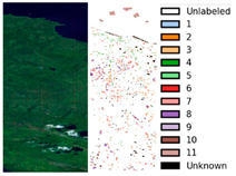
* denotes the data with the optimal performance in its category.

presents the classification results of the five comparative methods on the Dioni dataset, with corresponding visualization in Figure 12. The area within the red box contains unknown land cover types. It can be observed that the proposed method achieves the best performance in terms of recognition rates for Classes 4, 5, and 11 as well as overall evaluation metrics. Specifically, for Class 4 fruit trees, which are similar to other vegetation-covered areas, the recognition rate is generally very low due to its blurred boundaries and small number of learnable samples—models can only perform classification by extracting unique features of leaf reflectance. However, the du-al-branch network adopted in this study can extract richer features, thus achieving the highest recognition rate of 58.39% for Class 4. Classes 10 and 11 (seawater and shoal) have continuous and uniform texture features. Compared with heterogeneous features such as vegetation and buildings, they are less affected by spatial heterogeneity during classification, so their accuracy is higher than that of other classes. Multiple methods including the proposed method achieve 100% accuracy for these two classes. In addition, the proposed method uses prototype contrastive learning to enhance class discriminability. Meanwhile, due to the dual-branch network structure, features from the two task branches are merged in the shallow network, which can retain the basic in-formation of shallow features to a greater extent. This part of basic information contains discriminative information about unknown classes—information that traditional classification models are highly likely to ignore. By performing open-set classification based on this information, the proposed method outperforms single-branch networks in the OpenOA, OpenAA, and F1 metrics, reaching 90.36%, 91.05%, and 78.42%, respectively.

Although the dual-branch open-set classification method proposed in this paper achieves excellent performance in most categories, the inherent characteristics of its model structure impose inherent limitations on difficult categories such as Class 5 (shadow class) of the PaviaU dataset. The proposed method relies on a fusion judgment mechanism combining reconstruction error and prototype distance, along with a global threshold strategy. However, the “shadow class” inherently constitutes a heterogeneous and ambiguously characterized category due to its large intra-class spectral variability, high susceptibility to spectral confusion with building materials, and prevalent mixed pixel issues. This results in discrete distribution of its samples in the feature space, prone to high reconstruction errors, and their features tend to be close to the unknown-class prototypes constructed from ambiguous samples. Consequently, such samples are more likely to be misclassified as “unknown” or incorrectly categorized in the fusion judgment process. Therefore, the model faces challenges in balancing “maintaining classification accuracy of known classes” and “identifying unknown classes,” ultimately limiting its performance on such complex known categories. Future work will focus on introducing strategies such as spectral–spatial enhancement and few-shot learning to further improve the model’s discriminative capability for difficult categories.

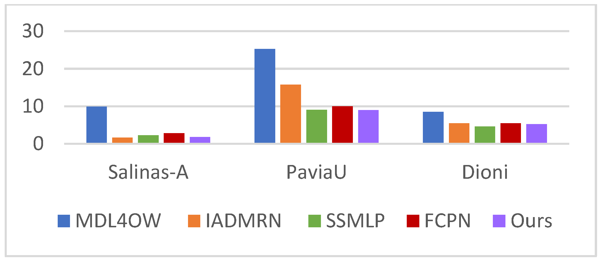
Since unknown classes overlap with known classes in either feature space or loss, both classifiers in generative models and discriminative boundaries defined by discriminative models will miss some unknown classes and misclassify known classes. This causes the overall classification accuracy of all methods to decrease when facing unknown classes; thus, the open-set classification robustness of the proposed model can be verified by the degree of accuracy reduction. A smaller degree of degradation indicates higher stability of the model when confronting unknown classes. In this paper, the class assignment of the training set is adjusted to conduct closed-set classification training, and the difference between the Overall Accuracy (OA) of closed-set classification and open-set classification is calculated. The results of each method on different datasets are shown in Figure 13.

It can be observed that the difference value of the proposed method remains at a relatively low level, indicating that the classification accuracy of the model for known classes is less likely to decrease due to disturbances from unknown classes in the open environment. To further verify the robustness of the model in open-set classification, for different datasets and with reference to paper [17], all samples of some known classes are selected as unknown classes to change the value of $Openness$, and the accuracy of open-set identification is observed.

Figure 14 illustrates the variation of unknown-class identification accuracy with $Openness$ for different methods across various datasets. Since different classes in the datasets have varying numbers of samples, the same value of $Openness$ can lead to different degrees of accuracy decline. Although the accuracy of the proposed method decreases as openness increases, the declining trend is relatively gentle, and the magnitude of decline is relatively small.

4.3. Visualization and Analysis of Unknown Classes

Since one of the assumptions of the proposed method is that the reconstruction performance for unknown classes is poor, we now analyze the original spectral curves and reconstructed spectral curves of the known class (trees) and unknown classes in the Pavia dataset. As shown in Figure 15, the same color represents the spectrum corresponding to the pixel at the same location.

It can be observed that the reconstructed spectral curves of the tree class still retain the typical vegetation spectral curve shape and are more compact, indicating small intra-class variation. In contrast, there are significant differences between the reconstructed spectral curves and original spectral curves of unknown classes. This analysis verifies the proposed method’s assumption that the reconstruction performance of unknown classes is poor, thus proving the effectiveness of the method. Meanwhile, it can be observed that the original spectrum and reconstructed spectrum of the third curve (cyan spectral line) among unknown classes are relatively similar, making it difficult to identify via reconstruction error alone. Therefore, the proposed method identifies unknown classes by combining reconstruction error and unknown-class prototype distance.

It can be observed that the reconstructed spectral curves of the tree class still retain the typical vegetation spectral curve shape and are more compact, indicating small intra-class variation. In contrast, there are significant differences between the reconstructed spectral curves and original spectral curves of unknown classes. This analysis verifies the proposed method’s assumption that the reconstruction performance of unknown classes is poor, thus proving the effectiveness of the method. Meanwhile, it can be observed that the original spectrum and reconstructed spectrum of the third curve (cyan spectral line) among unknown classes are relatively similar, making it difficult to identify via reconstruction error alone. Therefore, the proposed method identifies unknown classes by combining reconstruction error and un-known-class prototype distance.

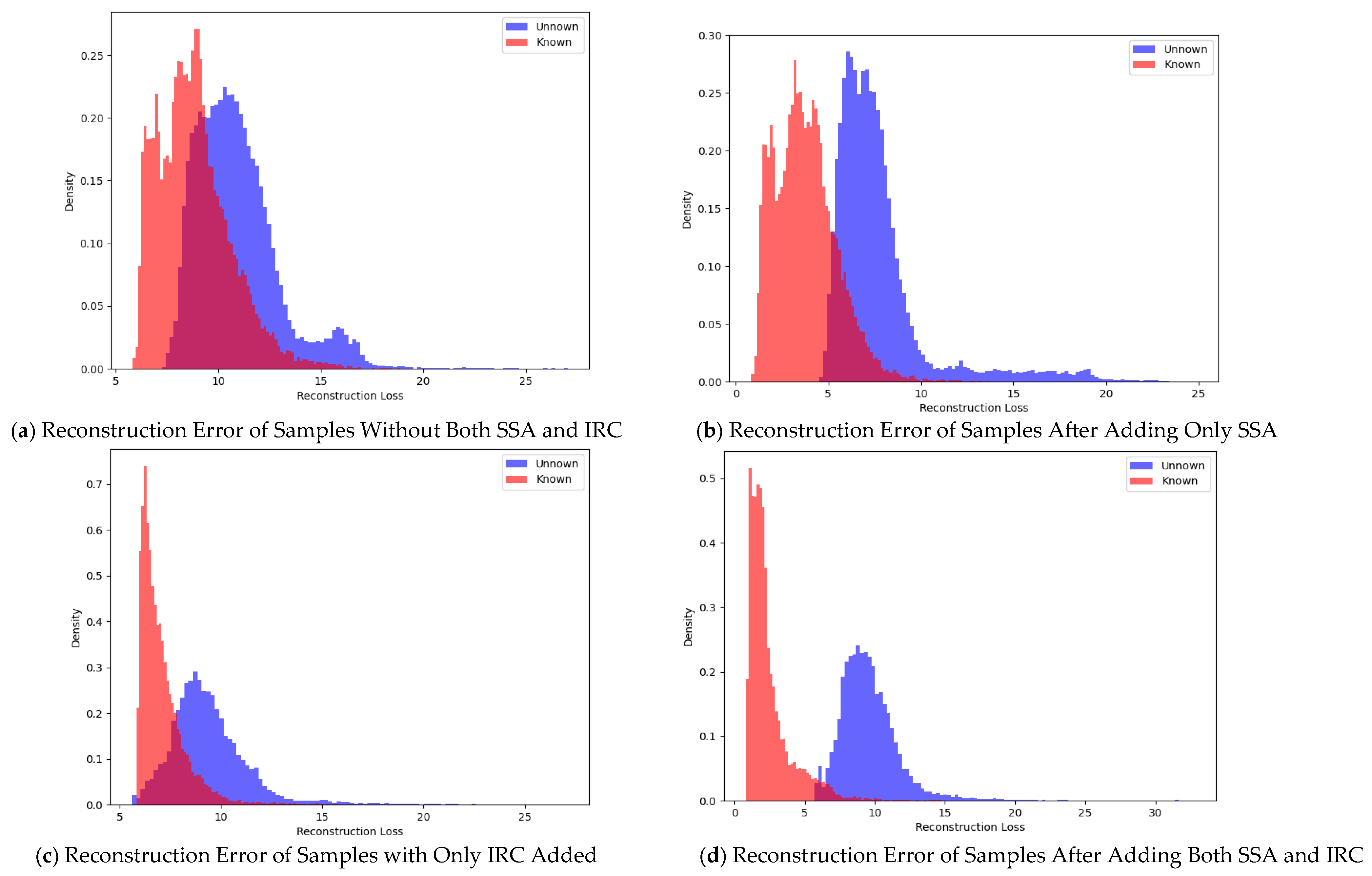
To verify whether the SSA layer and IRC layer in the reconstruction branch have a positive effect on reconstruction, this paper visualizes the reconstruction losses of known classes and unknown classes in the PaviaU dataset in the form of histograms before and after adding SSA and IRC, as shown in Figure 16.

Another assumption of the proposed method is that the confidence of unknown classes is generally lower than that of known classes. Therefore, samples with low confidence are averaged to construct unknown-class prototypes, and contrastive loss is then used to push known-class prototypes away from unknown-class prototypes, achieving the separation of known and unknown classes at the feature level. To validate the effectiveness of the proposed method, the output feature dimension of the network was adjusted to 2 in this subsection. After training on the PaviaU dataset, 200 samples are randomly selected from each known class and unknown class in the test set to observe their feature distribution, as shown in Figure 17.

It can be observed that unknown classes are distributed around unknown-class prototypes and at the edges of known-class prototypes, while most known classes cluster around their corresponding class prototypes. In prototype classification, the probability of a sample belonging to a class is calculated by dividing the distance between the sample and the prototype of that class by the sum of the distances between the sample and the prototypes of all classes. Features of unknown-class samples lie in the gaps between class prototypes, meaning the sample has roughly equal distances to at least two class prototypes. Its probability of belonging to these two classes is similar, with the probability corresponding to each class being less than 0.5. Thus, such samples have high uncertainty, corresponding to large information entropy and low confidence. In contrast, features of known-class samples cluster around their respective class prototypes and have the smallest distance to the prototype of their true class, resulting in low uncertainty and high confidence.

To verify the effectiveness of the proposed method, MDL4OW with a dual-branch structure is used as the baseline method. Experimental results across the three datasets—considering the addition or non-addition of the SSA and IRC modules, and the addition or non-addition of the PCL—are presented in

Table 5. Results of Ablation Experiments on Each Module for Open-Set Classification.

Datasets	Metric	Baseline Method	+SSA+IRC	+PCL	+SSA+IRC+PCL
Salinas-A	UDR	84.57	85.01	84.63	86.6 *
	Close-OA	92.53	92.97	95.65	95.81 *
	Open-OA	89.03	90.91	92.85	93.24 *
	Open F1	82.15	83.79	82.75	84.85 *
Pavia University	UDR	62.47	73.25	70.69	77.35 *
	Close-OA	87.76	88.65	89.88	91.13 *
	Open-OA	78.42	83.25	83.67	86.05 *
	Open F1	72.97	76.78	75.87	77.92 *
Dioni	UDR	57.21	58.35	57.06	58.12 *
	Close-OA	86.87	86.94	88.39	90.19 *
	Open-OA	84.67	87.01	86.85	89.66 *
	Open F1	53.68	55.78	54.12	59.85 *

* denotes the data with the optimal performance in its category.

. It can be observed that across all datasets, after adding the SSA and IRC modules, both the UDR and OpenOA are improved, as these modules reduce the overlapping region of reconstruction errors between known and unknown classes. After adding only the PCL module, the model’s performance in both Close-OA and OpenOA is significantly enhanced. This is because the PCL module increases the inter-class distance and enables the model to identify unknown classes using both prototype-based and reconstruction-based strategies. When the SSA, IRC, and PCL modules are added simultaneously, the combined method achieves the optimal performance across all metrics. This is attributed to the fact that high-quality reconstruction yields more representative compressed features, which helps the prototype classification network retain rich feature information.

5. Conclusions

SatIoT integrates satellite communication and IoT technologies to break the barriers in the hyperspectral remote sensing data chain of acquisition-transmission-analysis, enabling real-time acquisition and wide-area coverage of hyperspectral images and making such images the significant data support for refined decision-making in fields like geological exploration and environmental monitoring. Meanwhile, it also puts forward an urgent demand for intelligent classification of hyperspectral data in open environments, and how to efficiently and accurately classify known land cover types and reliably detect unknown ones remains a key problem to be solved in hyperspectral applications of SatIoT. However, existing hyperspectral open-set classification methods with a single strategy are limited by the one-sidedness of their discriminative logic, often facing issues such as misclassification of unknown classes and poor cross-region robustness, which makes them difficult to adapt to the dynamically changing land cover monitoring scenarios in SatIoT. Targeting this core pain point, this study proposes a dual-branch framework fusing reconstruction and prototype classification. The dual-branch architecture of the model achieves effective complementarity between reconstruction and prototype classification: the reconstruction branch improves the reconstruction accuracy of known classes through the SSA layer and IRC module, and the prototype classification branch constructs unknown-class prototypes based on confidence and enhances inter-class separability using Mahalanobis distance and contrastive loss. The proposed method demonstrates superior performance. On the three datasets of Salinas-A, PaviaU, and Dioni, its Unknown Detection Rate UDR, Open Set Overall Accuracy OpenOA, and open-set F1 score all outperform four comparative methods including MDL4OW. On the Salinas-A dataset, its OpenOA reaches 93.83%, and the difference between closed-set and open-set accuracy is only 1.82%. On PaviaU, the recognition rate of Class 4 reaches 99.54%. On Dioni, the recognition rate of Class 4 small-sample class is better than that of comparative methods; moreover, as openness increases, the unknown-class identification accuracy decreases gently, showing outstanding robustness and generalization. Visualization analysis further confirms the effectiveness of the method: the reconstructed spectral features of known classes are compact, while the reconstruction differences of unknown classes are significant; in the feature space, known classes form clusters, and unknown classes are explicitly separated; the pseudo-color label map has the highest degree of agreement with the real label map, with the fewest misclassifications of unknown classes. Ablation experiments show that the synergy of various modules improves classification performance. With MDL4OW as the baseline, the SSA+IRC modules increase UDR and OpenOA by up to 10.78% and 4.83%, respectively; the PCL module increases Closed Set Overall Accuracy Close-OA and OpenOA by up to 3.12% and 5.25%, respectively; the combination of the two achieves optimal metrics, confirming the rationality of the dual-branch architecture. The method proposed in this paper provides an effective solution for complex hyperspectral data processing in the open environment of SatIoT.

The dual-branch open-set classification method proposed in this paper still has certain limitations. Firstly, in terms of model structure, the parallel operation of the dual-branch and the introduction of multiple modules result in high computational complexity and a large number of parameters, making it difficult to meet the real-time processing requirements of remote sensing edge platforms such as satellites and unmanned aerial vehicles (UAVs) [33,34,35,36,37]. Secondly, the method is sensitive to the quantity and quality of training samples. In scenarios with insufficient samples or class imbalance, the model struggles to learn robust prototypes and clear reconstruction boundaries. Additionally, its strategy of determining the discrimination threshold for unknown classes based on global statistics is difficult to adapt to known classes with large intra-class variations and ambiguous features, which easily leads to misjudgment and limits its generalization ability in complex open scenarios. To address the above issues, future research can combine neural architecture search and knowledge distillation techniques to design lightweight spatial–spectral joint attention modules and hierarchical prototype alignment mechanisms, aiming to reduce model complexity while ensuring performance. Meanwhile, exploring model quantization and hardware acceleration technologies will promote the efficient deployment of the algorithm on edge platforms. Further introducing few-shot learning strategies is expected to optimize the classification performance of few-shot and unknown classes while reducing computational overhead, thereby providing more solid technical support for upgrading the precise perception capabilities of the SatIoT.