Article

Arbitrary-Scale Planetary Remote Sensing Super-Resolution via Adaptive Frequency–Spatial Neural Operator

by
Hui-Jia Zhao
1,
Xiao-Ping Lu
1,2,* and
Kai-Chang Di
3
1
School of Computer Science and Engineering, Macau University of Science and Technology, Taipa, Macau 999078, China
2
State Key Laboratory of Lunar and Planetary Sciences, Macau University of Science and Technology, Taipa, Macau 999078, China
3
State Key Laboratory of Remote Sensing and Digital Earth, Aerospace Information Research Institute, Chinese Academy of Sciences, Beijing 100101, China
*
Author to whom correspondence should be addressed.
Remote Sens. 2025, 17(22), 3718; https://doi.org/10.3390/rs17223718
Submission received: 24 September 2025 / Revised: 2 November 2025 / Accepted: 12 November 2025 / Published: 14 November 2025

Highlights

What are the main findings?
  • This study proposes AFSNO, an arbitrary-scale super-resolution model specifically designed for planetary remote sensing, which effectively preserves high-frequency geological details.
  • This study proposes Ceres-1K, the planetary super-resolution dataset comprising 1000 Ceres surface images.
What are the implications of the main findings?
  • AFSNO achieves competitive performance in both perceptual quality and quantitative metrics, and addresses the needs of planetary remote sensing.
  • The local attribution maps demonstrate that AFSNO can reconstruct images with large receptive fields.

Abstract

Planetary remote sensing super-resolution aims to enhance the spatial resolution and fine details from low-resolution images. In practice, planetary remote sensing is inherently constrained by sensor payload limitations and communication bandwidth, resulting in restricted spatial resolution and inconsistent scale factors across observations. These constraints make it impractical to acquire uniform high-resolution images, thereby motivating the need for arbitrary-scale super-resolution capable of dynamically adapting to diverse imaging conditions and mission design restrictions. Despite extensive progress in general SR, such constraints remain under-addressed in planetary remote sensing. To address those challenges, this article proposes an arbitrary-scale super-resolution (SR) model, the Adaptive Frequency–Spatial Neural Operator (AFSNO), designed to address the regional context homogeneity and heterogeneous surface features of planetary remote sensing images through frequency separation and non-local receptive field. The AFSNO integrates Frequency–Spatial Hierarchical Encoder (FSHE) and Fusion Neural Operator in a unified framework, achieving arbitrary-scale SR tailored for planetary image characteristics. To evaluate the performance of AFSNO in planetary remote sensing, we introduce Ceres-1K, the planetary remote sensing dataset. Experiments on Ceres-1K demonstrate that AFSNO achieves competitive performance in both objective assessment and perceptual quality while preserving fewer parameters. Beyond pixel metrics, sharper edges and high-frequency detail enable downstream planetary analyses. The lightweight, arbitrary-scale design also suits onboard processing and efficient data management for future missions.

Graphical Abstract

1. Introduction

High-resolution (HR) images are essential in planetary remote sensing [1,2,3,4,5,6,7,8,9,10,11]. These HR images enable researchers to reveal various geological features, including the tectonics and impact history of planets and asteroids [12,13]. While spacecraft and deep space exploration advancements have facilitated orbital scanning of planetary surfaces, acquiring HR images requires more sophisticated and heavier remote sensors. This increase in payload mass impacts spacecraft performance and overall mission complexity. For instance, the framing camera unit on the Dawn orbiter weighed only 5.5 kg [14]. Remote sensors also must balance spatial resolution and coverage, which significantly constrains the image quality obtained from orbiters. Additionally, adverse imaging conditions such as extreme temperatures and cosmic radiation impair the imaging process. In deep-space missions, the very long communication distances and limited data transmission bandwidth further restrict imaging system design and transmitted image quality. Compared to the complexity of directly acquiring HR images, super-resolution (SR) reconstruction from low-resolution (LR) measurements offers an efficient alternative, yielding finer details and better image quality. However, unlike natural image SR scenarios, planetary remote sensing poses significant domain-specific challenges.
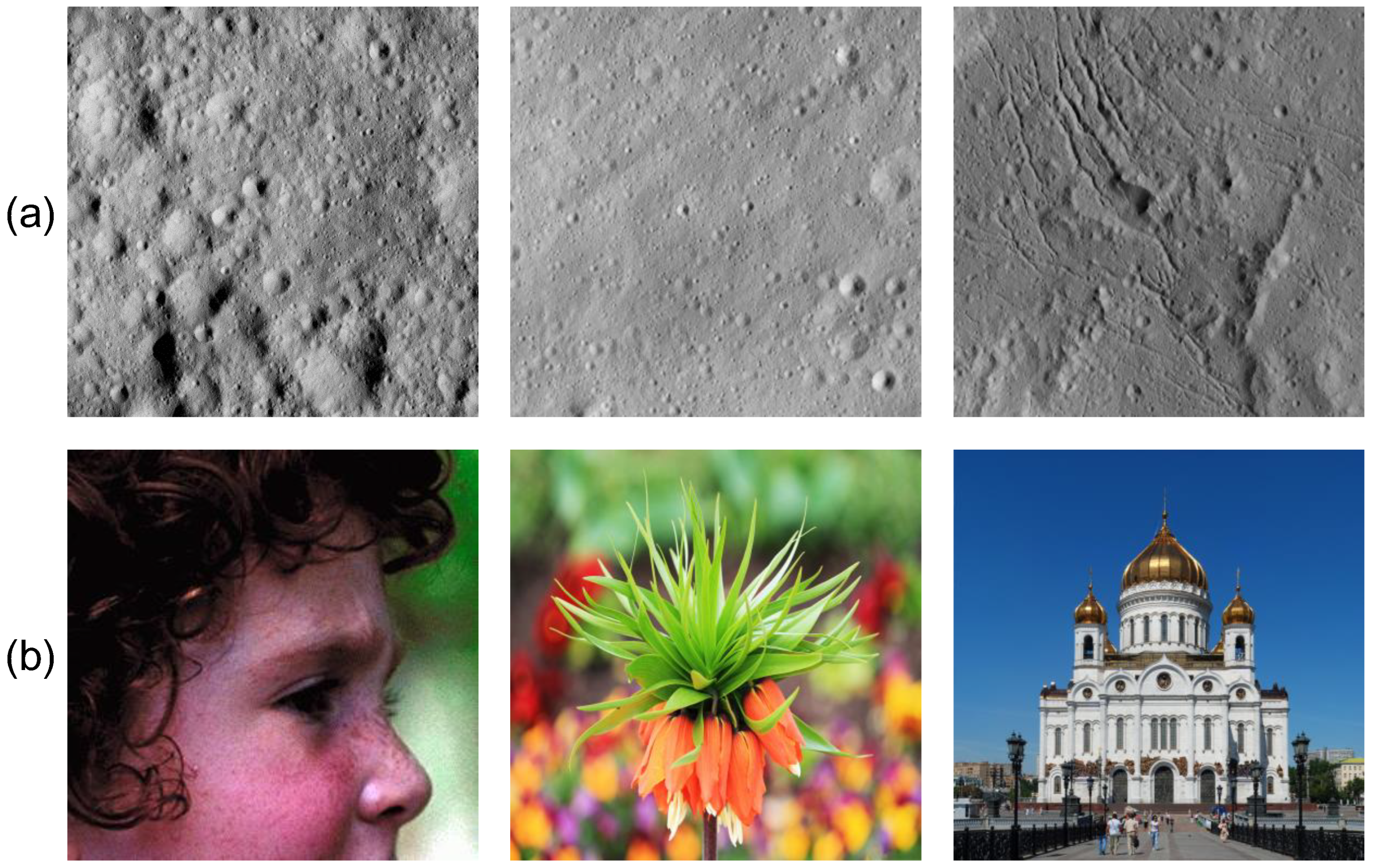
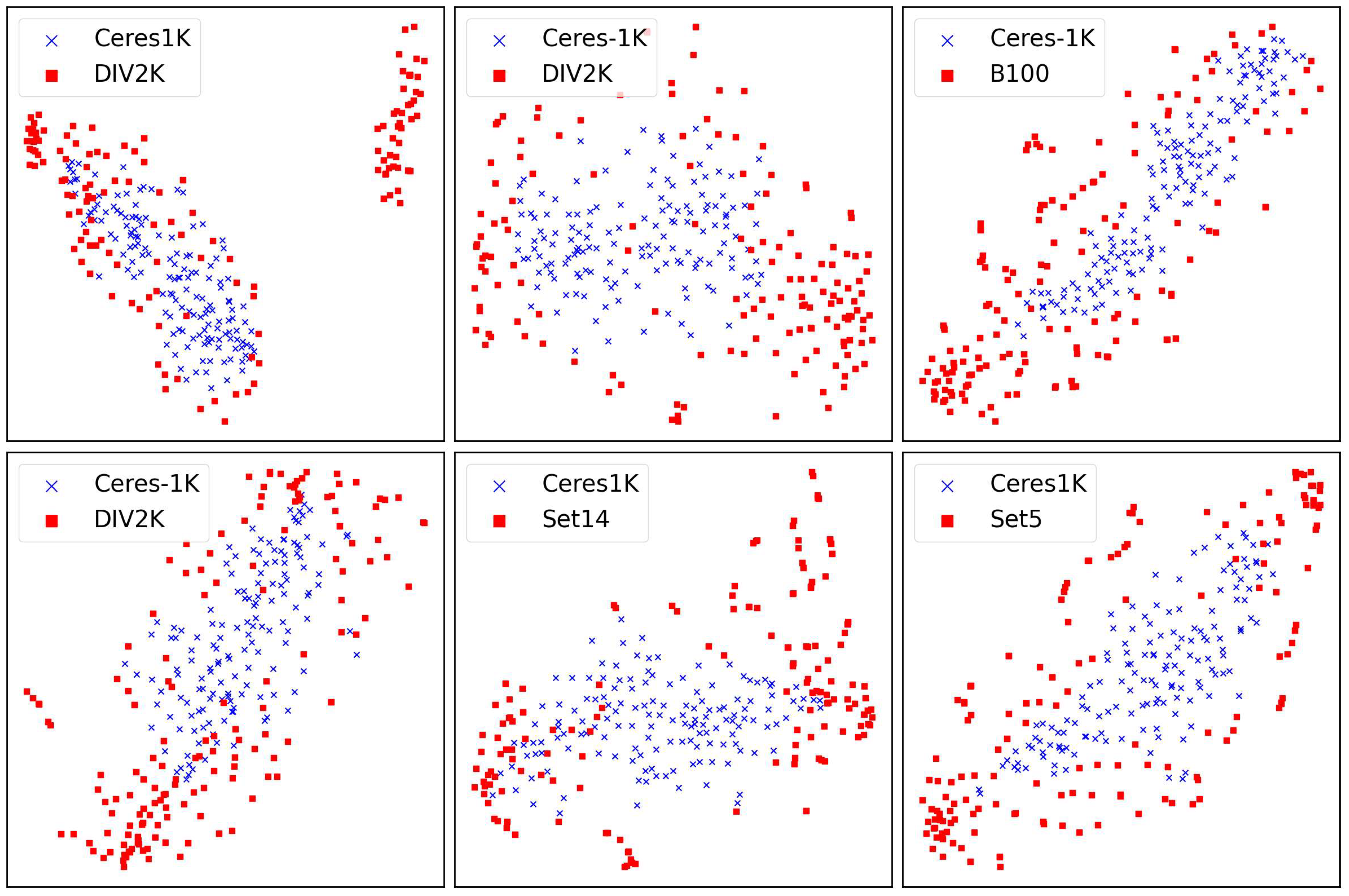
Firstly, planetary remote sensing images exhibit distinct characteristics compared to natural images. Current super-resolution (SR) methods primarily target natural images from datasets such as DIV2K [15], a widely used high-quality dataset containing 1000 diverse 2 K-resolution images; Set14, a benchmark dataset consisting of 14 images with varied content and structures; and Set5, a classic benchmark comprising 5 standard test images [16,17,18,19,20,21,22]. Remote sensing SR mainly focuses on the Earth observation images [23,24,25]. However, as illustrated in Figure 1 and Figure 2, which include example images and t-distributed stochastic neighbor embedding (t-SNE) visualizations, planetary remote sensing images display regional context homogeneity due to recurring semantic elements such as linear structures, impact craters, and domical features. Since the degree of context homogeneity varies across the whole planetary remote sensing image, neural networks must capture large-area contextual information. Consequently, modeling non-local receptive fields become critical for planetary SR tasks. Additionally, planetary remote sensing images often contain heterogeneous features, such as impact craters, linear structures, domical features, and lobate flows [13]. Linear structures and craters manifest as high-frequency components owing to abrupt edge transitions and rapid topographic changes. The coexistence of diverse geological features within localized regions introduces significant numerical disparities between high-frequency and low-frequency components, complicating direct reconstruction. To address this, neural networks must decompose geological features and perform multi-scale feature extraction. Furthermore, preserving edge details and high-frequency components is essential for accurate topographic analysis and sharp landform reconstruction.
Secondly, multi-scale enhancement is critical for scientific applications. Planetary remote sensing requires image enhancement across multiple scales to resolve varying levels of surface detail [23], necessitating SR models capable of arbitrary-scale processing within a unified framework. However, existing arbitrary-scale SR models predominantly rely on multilayer perceptron (MLP) for feature mapping, which may inadequately represent high-frequency image components [20,21,26,27]. Developing arbitrary-scale SR models that mitigate frequency bias is necessary. Moreover, space missions often generate vast datasets, and SR models with excessive parameters demand substantial computational resources. Lightweight architectures offer potential for onboard processing in future development [28].
Thirdly, standard datasets in planetary remote sensing are lacking. Validating model performance (for tasks such as SR, segmentation, and classification) requires standard benchmark datasets. The absence of such datasets hinders research advancement and model evaluation. To address this limitation, we construct Ceres-1K, the planetary remote sensing SR dataset, comprising high-resolution images from the Dawn mission’s exploration of Ceres.
Although deep learning-based SR methods have shown significant results, they still face several challenges when addressing planetary remote sensing needs. The combination of convolutional neural networks (CNNs) and residual connections has produced strong outcomes in both natural and remote sensing images [16,29,30,31,32,33]; however, these methods primarily focus on fixed-scale super-resolution, which restricts scientific analysis capabilities. Additionally, generative adversarial networks (GANs) have demonstrated good visual performance in reconstructing remote sensing images [25,34,35], yet they may generate artificial textures that compromise data integrity. Moreover, existing arbitrary-scale SR methods predominantly employ MLPs to map high-dimensional features into color space [20,22,23,36]. However, MLPs show limited capacity for learning high-frequency information [21,27], which is essential for reconstructing edge structures. Furthermore, most current remote sensing SR models are designed for Earth observation images, whose geomorphology differs significantly from planetary remote sensing images. For planetary remote sensing, scientific analysis such as surface age dating, structural mapping, and unit classification depend critically on resolving crater rims, lineaments, and small-scale textures Russell et al. [12], Buczkowski et al. [13]. Enhanced reconstruction of high-frequency content is therefore not only a perceptual improvement but directly impacts tasks such as crater size–frequency distribution counting, fracture extraction, and geomorphologic mapping. This necessitates the development of SR models specifically tailored to planetary remote sensing characteristics, capable of addressing regional context homogeneity, decomposing heterogeneous geological features, and mitigating frequency bias. Additionally, lightweight architectures with reduced parameters are essential to enable onboard data pre-processing for future space missions.
To address these challenges, we propose the Adaptive Frequency–Spatial Neural Operator (AFSNO), an arbitrary-scale SR framework. The AFSNO introduces two key innovations: frequency-domain feature reconstruction and a feature redundancy suppression module. While frequency transforms such as Discrete Fourier Transform (DFT) and Discrete Cosine Transform (DCT) are widely utilized to enhance neural network feature representation [21,37,38,39], existing SR methods typically reconstruct entire frequency-domain features directly. This approach risks neglecting high-frequency components due to the numerical gap between frequency bands. To resolve this, AFSNO incorporates the High-Frequency Reconstruction Group (HFRG) with a frequency-band separation mechanism to avoid the numerical gap between different frequency components, which also facilitates the decomposition of heterogeneous geological features based on their distinct geomorphic change rates. The Global Reconstruction Group further enhances non-local receptive fields through frequency domain feature processing, enabling context homogeneity modeling. Subsequently, the proposed parallel fusion mechanism integrates the extracted features with the Galerkin-type attention outputs, thereby generating the comprehensive final representation. Conventional architectures, such as ResNet and DenseNet, frequently retain redundant feature representations, leading to increased computational costs. We therefore propose Enhanced Spatial and Channel Blocks (ESCB), which employ specialized normalization layers to suppress spatial deviations and reduce redundant features. The FSHE encoder combines ESCB with sequential spatial-frequency feature integration to achieve multi-scale feature extraction. Beyond the network structure, there remains a lack of planetary remote sensing datasets for validating SR and other tasks. Ceres, the largest object in the asteroid belt, exhibits diverse surface features such as impact craters, linear faults, and bright deposits. Understanding its geological diversity aids in validating SR methods for planetary remote sensing. We also build Ceres-1K dataset.
The main contributions of this work can be summarized as follows:
1.
We present the AFSNO, a model that learns the mapping function between HR and LR image function spaces. This arbitrary-scale SR framework integrates the FSHE and Fusion Neural Operator, enabling single-model arbitrary-scale super-resolution.
2.
We propose the Frequency–Spatial Hierarchical Encoder (FSHE), which enables multiscale feature extraction while suppressing redundant features bridge the gap to efficient SR for scientific applications. Additionally, we propose the Fusion Neural Operator with a parallel frequency–spatial fusion structure that decomposes geological features and reduces frequency bias to accommodate planetary remote sensing image characteristics.
3.
We present Ceres-1K, the planetary remote sensing dataset compiled from images of the dwarf planet Ceres. The dataset contains 1000 images encompassing diverse surface geomorphologies, addressing the absence of benchmark data for planetary SR. Extensive experiments on Ceres-1K confirm the effectiveness of the AFSNO.

2. Related Works

2.1. Deep Learning Based SR Methods

Convolutional Neural Networks (CNNs) have achieved substantial progress in computer vision tasks. For SR, CNN-based models surpass traditional methods in enhancing image quality [16,17,19,32,33,40,41,42,43,44]. The RCAN introduced residual channel attention mechanisms to adaptively weight features across channels [32]. SwinIR established a robust transformer-based backbone [18], and HAT improved reconstruction by integrating channel and self-attention mechanisms [45]. However, these models typically operate at fixed scales. Meta-SR addressed this limitation by enabling arbitrary-scale SR through dynamic weight prediction [46]. Continuous image representation further advanced arbitraryscale reconstruction [20,22,27]. Representing image textures in 2D Fourier features has also demonstrated effective performance [21]. Beyond spatial SR, hyperspectral image SR has also achieved notable spectral super-resolution results [8,9,10,11]. The introduction of spectral dictionaries reformulated hyperspectral image SR as a variational regularization problem [11]. Simulating self-similarities between high-resolution (HR) and low-resolution (LR) images has also demonstrated promising performance [10]. Model-guided crossfusion networks have been proposed for spectral super-resolution, explicitly leveraging cross-network feature fusion to improve reconstruction quality [8].

2.2. Spectral Bias

Spectral bias refers to the limited ability of MLP to learn high-frequency components [26,47], resulting in losing fine details during reconstruction, a critical issue for planetary remote sensing. While MLP remains central to arbitrary-scale SR for mapping latent features to color space [20,27], prior solutions include Fourier space texture characterization and frequency domain coordinate projections [21,47].

2.3. Efficient Convolution Design

Rather than indiscriminately constructing deeper neural networks, rigorously developed lightweight models have demonstrated significant capabilities. The introduction of sparsely connected groups to redesign convolution enables the fusion of information from different representation subspaces [31]. The parallel structure and group convolution techniques also reduce computational resource requirements [48,49]. TVConv specifically addresses interrelated pixel relationships between images [50], while SCConv works to reduce redundant features, achieving effective neural networks with fewer model parameters [51]. By combining Fast Fourier Transform with ReLU activation functions, researchers have constructed plug-and-play blocks that enable models to achieve non-local receptive fields [37].

3. Methodology

This section describes the structure and components of AFSNO. We first present an overview of the AFSNO architecture in Section 3.1. Next, we detail the FSHE in Section 3.2. Section 3.3 describes the Lift module, a crucial component of our network. We then explain the Fusion Neural Operator in Section 3.4, followed by an examination of the Edge-Aware Frequency Loss in Section 3.5.

3.1. Overview Pipeline

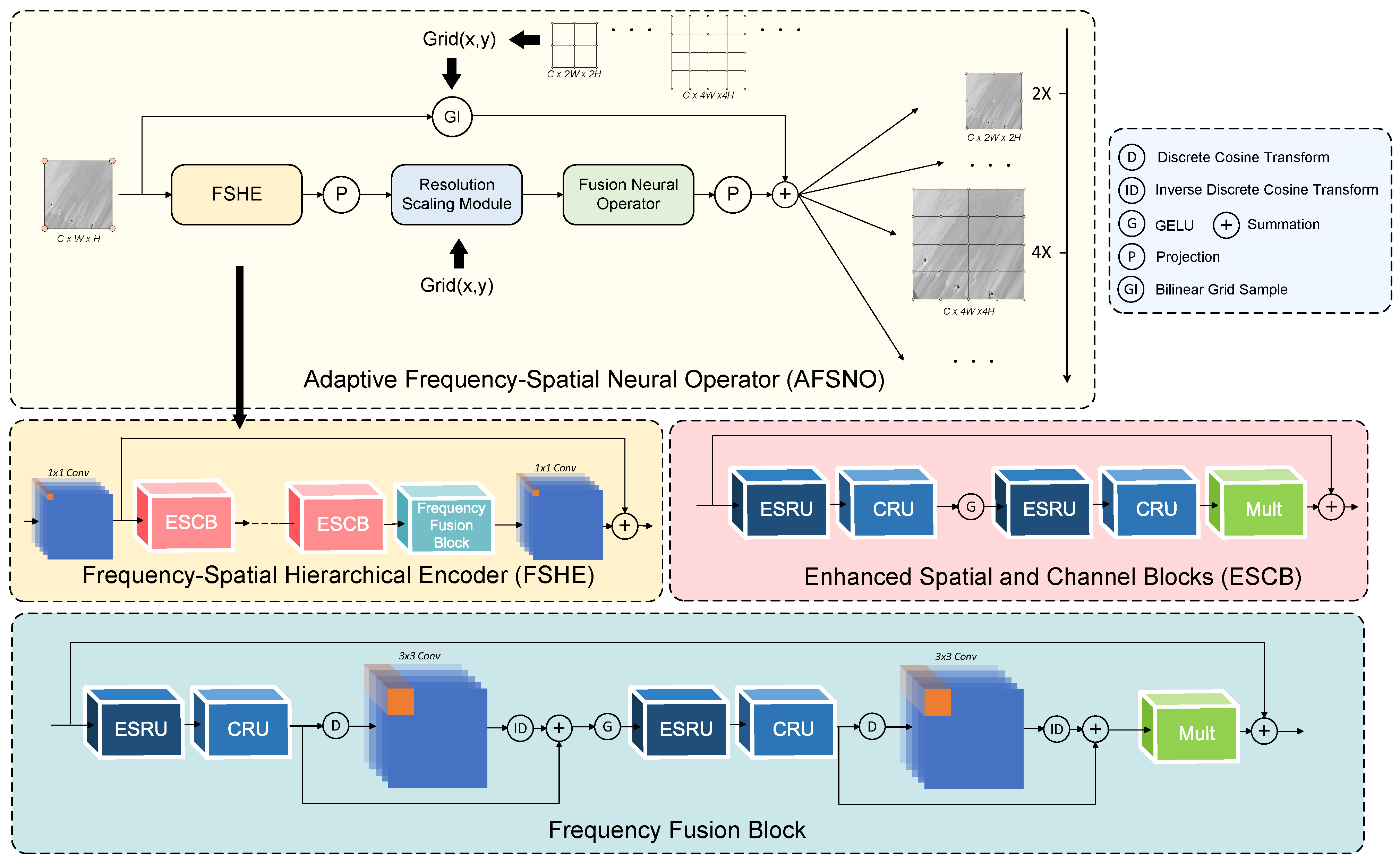
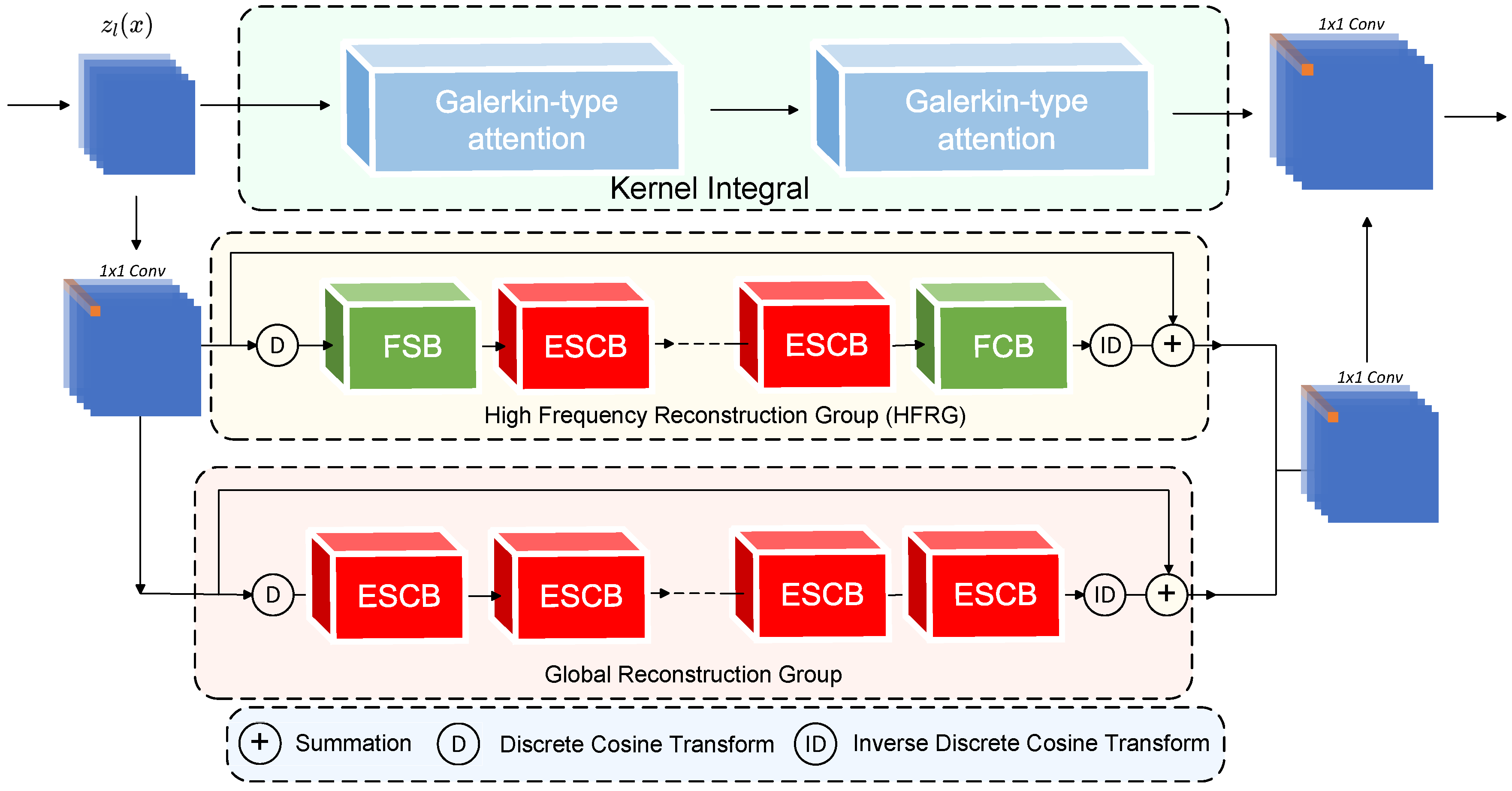
The structure of the AFSNO is shown in Figure 3. The input image is transformed into a latent feature space through FSHE. This network consists of multiple ESCB, Frequency Fusion Block, and 1 × 1 Convolution. The image is first extracted by the 1 × 1 Convolution as follows:
x = C o n v ( I L R ) ,
where C o n v ( ) denotes the 1 × 1 Convolution. I L R represents the input LR image, which is mapped into the shallow latent space. The feature is further extracted by several ESCB and can be described as:
F d ( x ) = F E S C B ( F d 1 ( C o n v ( I L R ) ) ) = F E S C B ( F E S C B ( · · · F E S C B ( C o n v ( I L R ) ) · · · ) ) ,
where F E S C B denotes the ESCB, which enhances the neural network’s feature representation with low feature redundancy. F d ( C o n v ( I L R ) ) is the d-th ESCB. Subsequently, the feature is input into the Frequency Fusion Block. We further have:
E θ ( P L R ) = C o n v ( F F F B ( F d ( C o n v ( I L R ) ) ) ) ,
where FFB represents the Frequency Fusion block, capable of representing features in the frequency domain. Further details about ESCB and Frequency Fusion Block are presented in Figure 3. After the input image is extracted into the latent feature space by FSHE, the latent feature is resized to the target size by the Lift module. Finally, the latent feature is reconstructed using the Fusion Neural Operator:
I S R = F n o ( L i f t ( E θ ( I L R ) ) ) + G I ( I L R ) ,
where F C A N O denotes the Fusion Neural Operator in the AFSNO, and L ift refers to the Lift module. G I represents the Bilinear Grid Interpolation.

3.2. Frequency–Spatial Hierarchical Encoder

Network architectures such as DenseNet and ResNet often encompass numerous redundant features [51]. To mitigate redundancy and enhance the feature representation of the encoder, we build redundancy reduced convolution unit which named ESRU and introduce the Frequency Fusion block to capture the multi-scale information.

3.2.1. Suppression of Channel and Spatial Redundancy

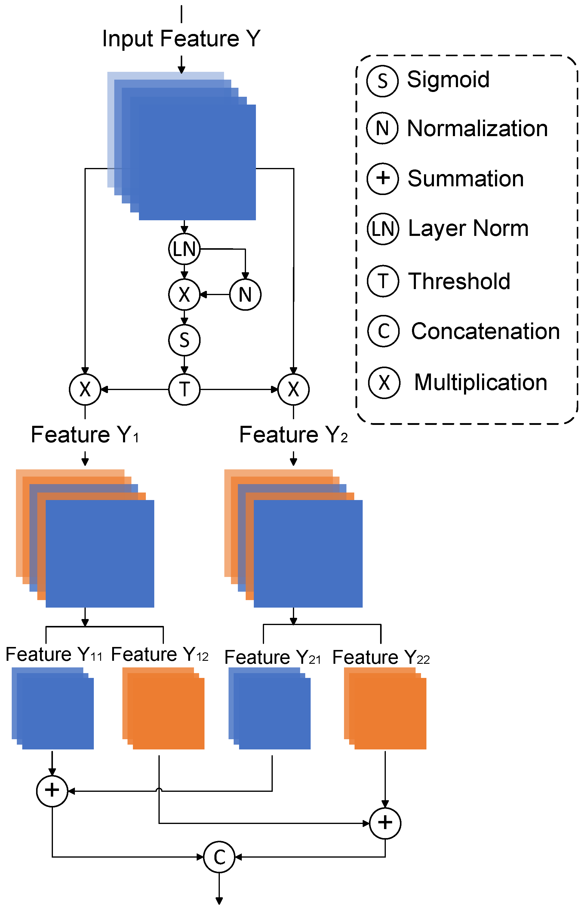
Convolutional feature redundancy remains a critical challenge in spatial and channel dimensions for image restoration. While SCConv’s spatial refinement unit (SRU) and channel refinement unit (CRU) partially addresses this issue in classification tasks [51], planetary remote sensing SR demands enhanced spatial adaptation due to non-stationary pixel correlations and preservation of high-frequency edge features. We therefore redesign the SRU to develop the Enhanced Spatial Refined Unit (ESRU) as Figure 4 shows, fundamentally redesigning the normalization strategy. Unlike batch normalization’s batch-statistics dependence that suppresses critical spatial deviations across correlated planetary terrains, ESRU implements layer normalization to perform sample-wise adaptive standardization—preserving local texture variations while stabilizing feature magnitudes.

3.2.2. Integration of Spatial and Frequency Features

The Frequency Fusion Block enables multi-scale feature extraction through frequency-domain hierarchical representation learning. A convolution applied in the frequency domain performs cross-frequency modulation, effectively fusing multi-scale characteristics through learnable frequency filters. The inverse DCT (IDCT) reconstructs spatial features while preserving scale-specific information through residual connections. Complemented by dynamic feature reconstruction in the ESRU and CRU. The Frequency Fusion Block achieves simultaneous preservation of contextual semantics and multi-scale feature aggregation.

3.3. Lift in Latent Space

Deep learning-based SR methods typically employ bicubic interpolation or transposed convolution layers for the upsampling step. However, direct application of bicubic interpolation to the LR image will introduce blocky artifacts [52]. The transposed convolution layers will cause crosshatch artifacts by the zero padding. Spatial grid interpolation and the Frequency–Spatial feature encode are combined to build the Resolution Scaling Module. In AFSNO, the Lift module performs resolution scaling in the latent feature space to enable arbitrary-scale super-resolution. Given the latent features Z R C × H × W extracted by FSHE and a target scale factor s R + , the Lift module rescales the spatial dimensions to s H × s W while preserving the channel-wise feature representation. Formally, the Lift operation is implemented through bilinear grid sampling:
Z = F interp ( Z , G s ) ,
where Z R C × ( s H ) × ( s W ) denotes the upsampled latent features, and F interp ( · , · ) represents the bilinear interpolation operator. The normalized coordinate grid G s R ( s H ) × ( s W ) × 2 is constructed by uniformly sampling spatial coordinates in the range [ 1 , 1 ] 2 :
G s [ i ,   j ] = 2 j s W 1 1 2 i s H 1 1 ,   i { 0 , , s H 1 } ,   j { 0 , , s W 1 } .
For each output position ( i , j ) in Z , the feature vector is computed via bilinear interpolation of the four nearest neighbors in Z:
Z : , i , j = ( p , q ) N ( i , j ) w p , q ( i , j ) · Z : , p , q ,
where N ( i , j ) denotes the set of four neighboring grid points, and w p , q ( i , j ) are the bilinear interpolation weights satisfying ( p , q ) w p , q ( i , j ) = 1 . Unlike traditional pixel-space upsampling that directly interpolates pixel values, the Lift module operates on high-dimensional latent features, enabling the subsequent Fusion Neural Operator to reconstruct fine-grained details from a resolution-aligned feature representation. This design decouples spatial scaling from semantic feature extraction, allowing arbitrary continuous scales s to be handled within a single unified framework without retraining.

3.4. Fusion Neural Operator

Following the upsampling process by the Resolution Scaling Module, image reconstruction is performed using the Fusion Neural Operator. This operator consists of three components: the Neural Operator, the Global Reconstruction Group, and the HFRG, which work collaboratively to reconstruct the image. The detailed structure is illustrated in Figure 5, Figure 6 and Figure 7. The Neural Operator module employs kernel integral to map features into the HR function space, implemented through Galerkin-type attention. The structure of Galerkin-type attention is shown in Figure 6. This attention mechanism is extensively used for mapping in finite dimensions [53]. Compared to convolution architectures, multilayer attention enables dynamic latent basis updates, essential for learning high-frequency components. The kernel integral approximated by Galerkin-type attention is described as:
( F ( z ) ) ( x ) = Θ F ( z ( x ) , z ( f ( x ) ) ) d f ( x ) i n W v · exp z ( x ) T W q T W k z i r z j n exp z ( j ) T W q T W k z i r z ,
where f ( · ) represents the mapping between corresponding LR and HR function spaces, and f ( x ) denotes the pair HR image with input x. The function z ( · ) represents the hidden representation of images. In the attention framework, W q , W k , W v R r z × r z denote the queries, keys, and values functions. The parameterized kernel integral ( F ( z ) ) ( x ) is approximated by the Fusion Neural Operator. Furthermore, the core mechanism of Galerkin-type attention can be described as follows, with details shown in Figure 6:
P = 1 H W W k W v ,   Y = W q P ,
where the normalization factor 1 / ( H W ) ensures scale invariance across different resolutions. The feature P aggregates spatial information via key-value interaction, and the output Y is obtained by projecting query features onto the learned prototype. After reshaping back to spatial format and applying residual connections with feedforward refinement, this formulation enables the Galerkin-type attention to dynamically update latent basis functions for learning high-frequency components in planetary images. After constructing parallel network structures with the Neural Operator, Global Reconstruction Group, and HFRG, the complete Fusion Neural Operator is expressed as:
( F ( z ) ) ( y ) = C [ Θ F ( z ( x ) , z ( f ( x ) ) ) d f ( x ) , G g ( z ( x ) ) , G s c ( z ( x ) ) ] ,
where G g ( z ( x ) ) and G s c ( z ( x ) ) represent the Global Reconstruction Group and HFRG, respectively. C denotes the fusion layer comprising GELU activation function and convolution layer.

3.4.1. Non-Local Receptive Field

In the frequency domain, any pixel change affects the entire image. The DCT basis provides linear spectrum representation while preserving global information. Unlike the High Frequency Reconstruction Group (HFRG), the Global Reconstruction Group applies a series of ESCB operations after the DCT without separating features into components. Furthermore, combining convolution and nonlinear activation functions achieves a non-local receptive field [37]. This approach enables the Fusion Neural Operator to capture context information from the entire image, which is crucial for reconstructing planetary remote sensing images.

3.4.2. Frequency Decomposition

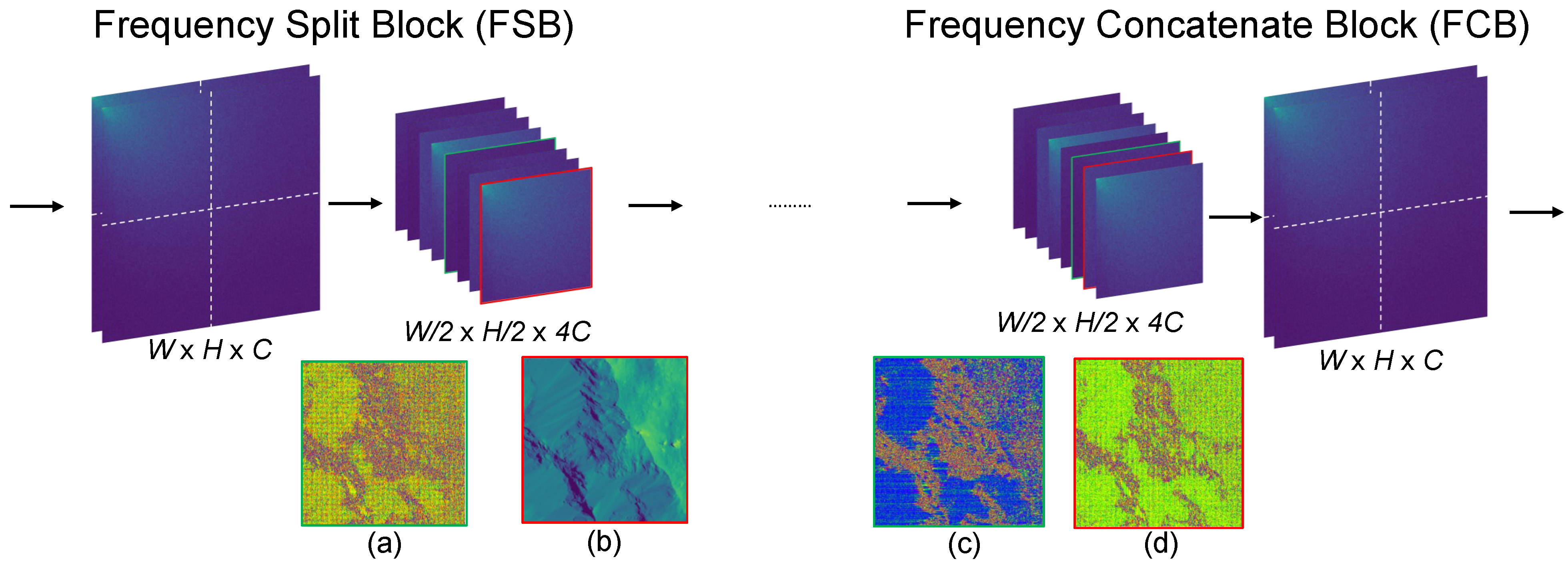
Frequency domain features exhibit a significant numerical gap between high-frequency and low-frequency components. Following the frequency distribution characteristics of DCT, HFRG employs frequency split block (FSB) and frequency concatenation block (FCB) (shown in Figure 7) to decompose frequency features into four distinct frequency bands. The network subsequently reconstructs these features separately, which effectively addresses the numerical gap between different features and helps mitigate spectral bias. Since different geological features often coexist within small areas, the numerical disparity between high-frequency and low-frequency components makes direct reconstruction challenging. Therefore, HFRG enables effective reconstruction of various geological features. This structure also supplies frequency information that helps reduce spectral bias. The parallel structure of HFRG, Global Reconstruction Group, and Neural Operator facilitates coordinated processing across different frequency components and in the spatial domain. The detailed HFRG architecture is presented in Figure 5 and Figure 7.

3.5. Edge-Aware Frequency Loss

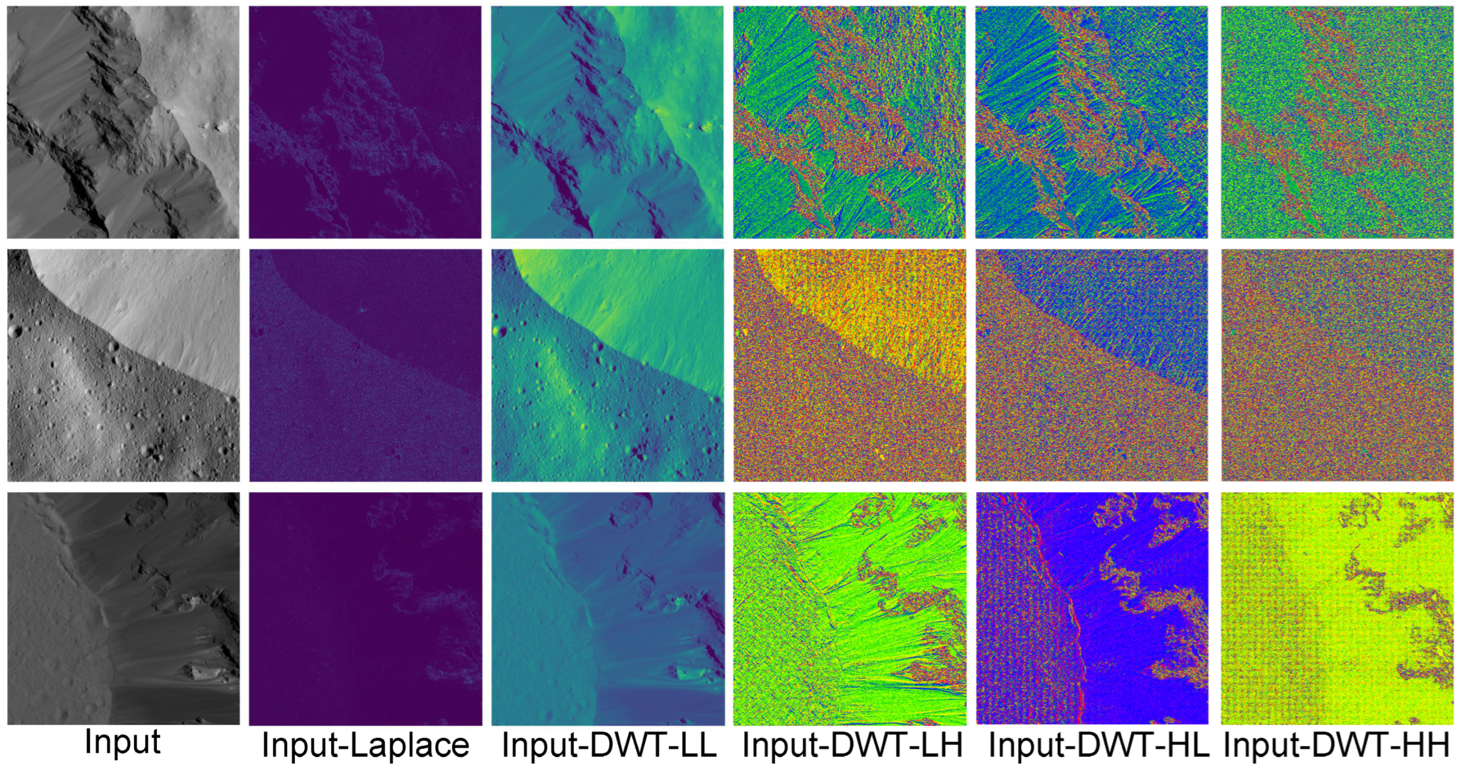
The discrete wavelet transform (DWT) decomposes a signal or image into multiple subbands as Figure 8 shows, which is particularly useful in SR tasks due to its ability to represent high-frequency information effectively [54]. Pixel-wise loss functions in SR tend to generate blurry images [37,52]. To address this limitation, we propose the Frequency Fusion Edge Loss Function that strategically combines the Charbonnier loss with the Laplace edge operator and DWT-based constraints. Specifically, the Charbonnier loss formulation is selectively applied to the Laplace edge term to enhance edge preservation robustness. The composite loss function is expressed as:
L ( λ 1 , λ 2 ) = i = 1 N x ^ i x i 1   +   λ 1 i = 1 N Δ x ^ i Δ x i 2 2 + ϵ 2   +   λ 2 i = 1 N Θ ( x ^ i ) Θ ( x i ) 1 ,
where the x ^ i , x i denote the i-th reconstruction image and i-th ground truth image. The symbol Δ also represents the Laplace operator, while Θ denotes the bior1.3 wavelet operator. The e p s refers to a fixed small constant. After conducting experiments, the values of λ 1 and λ 2 are fixed at 0.1 and 0.01.

4. Experiments

In this section, we first introduce the Ceres-1K dataset. We then present comparison experiments to validate the proposed AFSNO. Ablation studies are conducted to evaluate the effectiveness of each proposed module. Finally, we perform local attribution analysis to examine the receptive field of AFSNO.

4.1. Ceres-1K Dataset

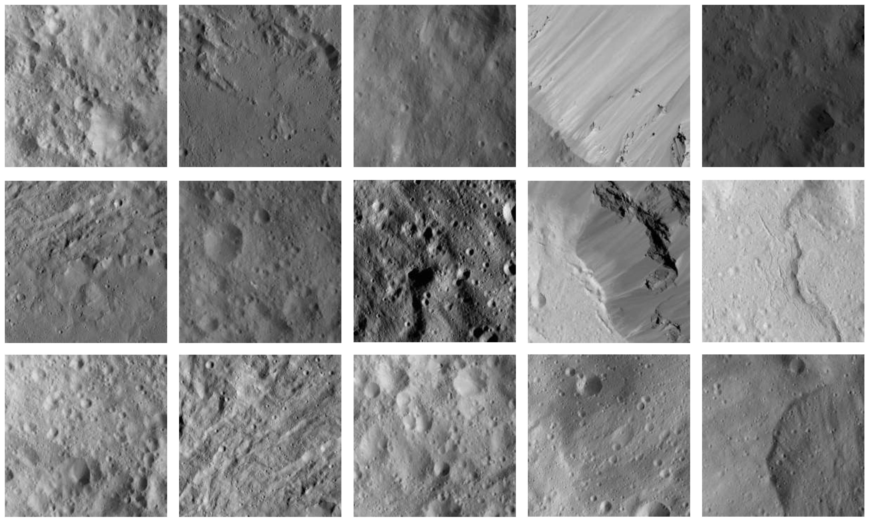
Ceres, a dwarf planet characterized by a silicate core, resides in the asteroid belt between Mars and Jupiter. Scientific understanding of Ceres remained limited until the Dawn spacecraft entered its orbital mission [12]. As the largest object in the asteroid belt with a diameter of approximately 940 km, Ceres exhibits a complex geological history recorded in its surface features. The planetary body displays diverse geological features shaped by both impact processes and internal geological activity, including kilometer-scale linear structures, impact craters, mounds, and domes [13]. Dawn mission observations revealed that Ceres’ surface preserves evidence of cryovolcanism, and potential subsurface ice. The Ceres-1K dataset is specifically designed to cover the principal landform classes whose accurate interpretation requires preservation of high-frequency edge details [13]. These include linear structures (Samhain Catenae), impact craters (Occator), lobate flows, domes (Ahuna Mons), and bright spots. The dataset comprises a total of 1000 images, partitioned into 900 training images and 100 testing images. All images were sourced from NASA’s Small Bodies Node (https://pdssbn.astro.umd.edu/, accessed on 19 October 2024), with spatial resolutions of 62 m/pixel (Figure 9).

4.2. Experimental Results

4.2.1. Implementation Details

The AFSNO and various other SR techniques were executed on a GPU platform comprising an NVIDIA V100 SXM3 32 GB GPU and an Intel Xeon Platinum 8168 CPU operating at 2.70 GHz. The code was conducted using the PyTorch. During the training phase, images were randomly segmented into 48 × 48 pixel patches and subsequently downsampled using the bicubic interpolation method. The AFSNO was trained with the Frequency Fusion Edge Loss function and the Adam optimizer. The learning rate adjustment was managed by a Gradual Warmup Scheduler, which incorporated a warmup multiplier of 10, spanned 150 warmup epochs, and culminated in a total of 1150 training epochs. The learning rate for AFSNO underwent a decay process governed by a cosine annealing learning rate schedule, starting with an initial value of 4 × 10 5 . The experimental results for Meta-SR, Local Implicit Image Function (LIIF), Adaptive Local Implicit Image Function (ALIIF), Local Texture Estimator (LTE), super-resolution neural operator (SRNO), and AFSNO were evaluated using a single model trained with a random scale uniformly sampled from ×1 to ×4. The patch sizes for LIIF, ALIIF, LTE, SRNO, and AFSNO were set to 48 × 48 . The training epoch was adjusted to fit the Ceres-1K Dataset. The training procedure is shown in Algorithm 1.
Algorithm 1 Training Procedure for AFSNO.
 1:
Input: Training dataset D T , Maximum epochs P
 2:
%Learning rate follows cosine annealing decay
 3:
Initialize: model parameters θ
 4:
for each I H R D T  do
 5:
    %Generate dataloader
 6:
    Randomly crop image patch I p H R from I H R
 7:
    Sample scale factor s U ( 1 , 4 ) from Uniform distribution
 8:
    Generate I p L R via bicubic downsampling with scale s
 9:
    Add pair to batch: B B { ( I p H R , I p L R ) }
10:
end for
11:
for epoch = 1 To P do
12:
    %Optimized model parameters θ
13:
    Compute L according to Equation (11)
14:
    Update model parameters θ using Adam optimizer
15:
end for
16:
return optimized parameters θ

4.2.2. Network Details

The encoder within the AFSNO framework, denoted as FSHE, is composed of 15 ESCBs and one Frequency Fusion Block, which together transform the input image into a 24-dimensional latent feature space. The HFRG and the Global Reconstruction Group each consist of 9 ESCBs and maintain both input and output dimensions at 24. Considering the shallow depth of the FSHE, the residual scaling factor of the proposed ESCBs is set to 1, which means no scaling is applied to residual connections, to maximize model capacity and expressivity.

4.2.3. Quantitative Result

Table 1 and Table 2 present a series of experimental results comparing enhanced deep residual networks (EDSR) [16], residual dense network (RDN) [33], holistic attention network (HAN) [17], SwinIR [18], LIIF [20], ALIIF [27], MetaSR [46], LTE [21], SRNO [22], and AFSNO. The experiment results demonstrate that AFSNO achieves competitive performance across most evaluated scales. Although the superiority of AFSNO diminishes with increasing scale, it can still be concluded that Fusion Neural Operator and FSHE improve AFSNO’s capacity to effectively learn the mapping between corresponding function spaces. In the SRNO, LIIF, ALIIF, LTE, and Meta-SR, the encoder adopts the EDSR-baseline. Table 3 demonstrates that AFSNO achieves inference with lower floating-point operations per second (FLOPs) compared to other arbitrary-scale SR models.

4.2.4. Qualitative Result

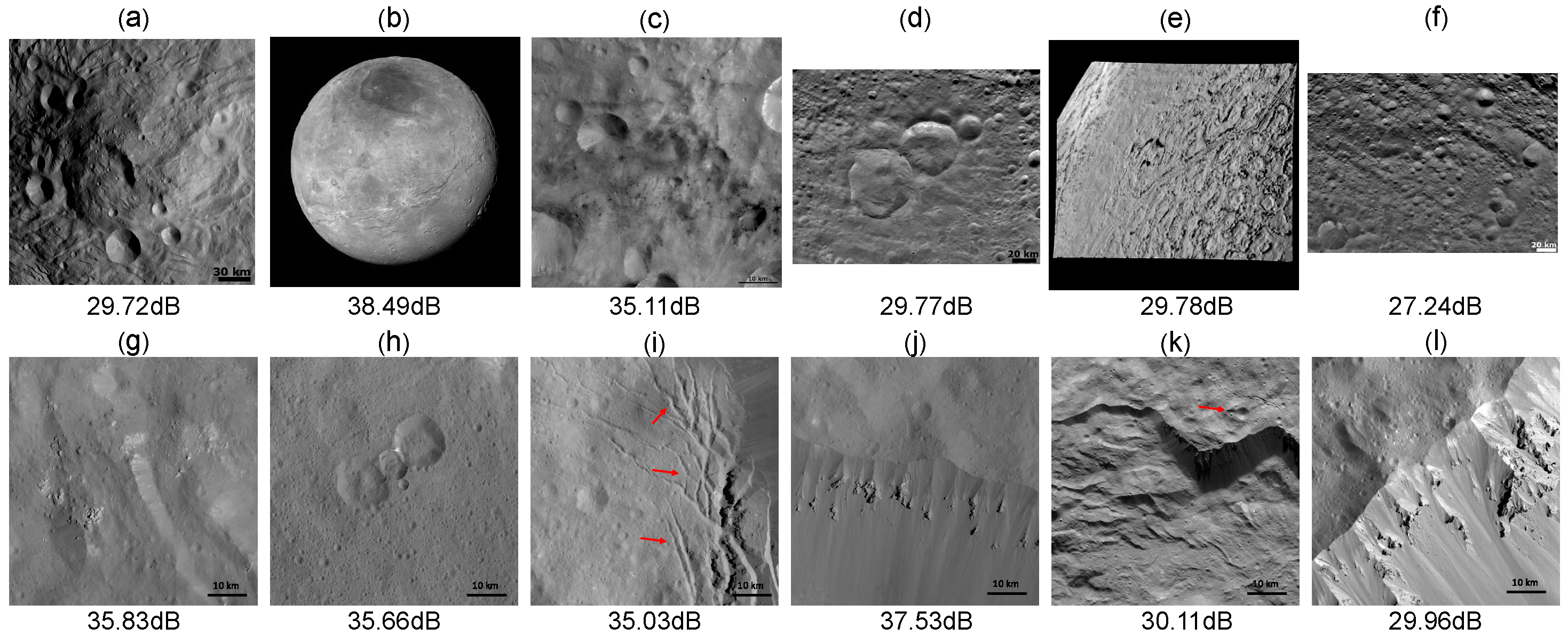
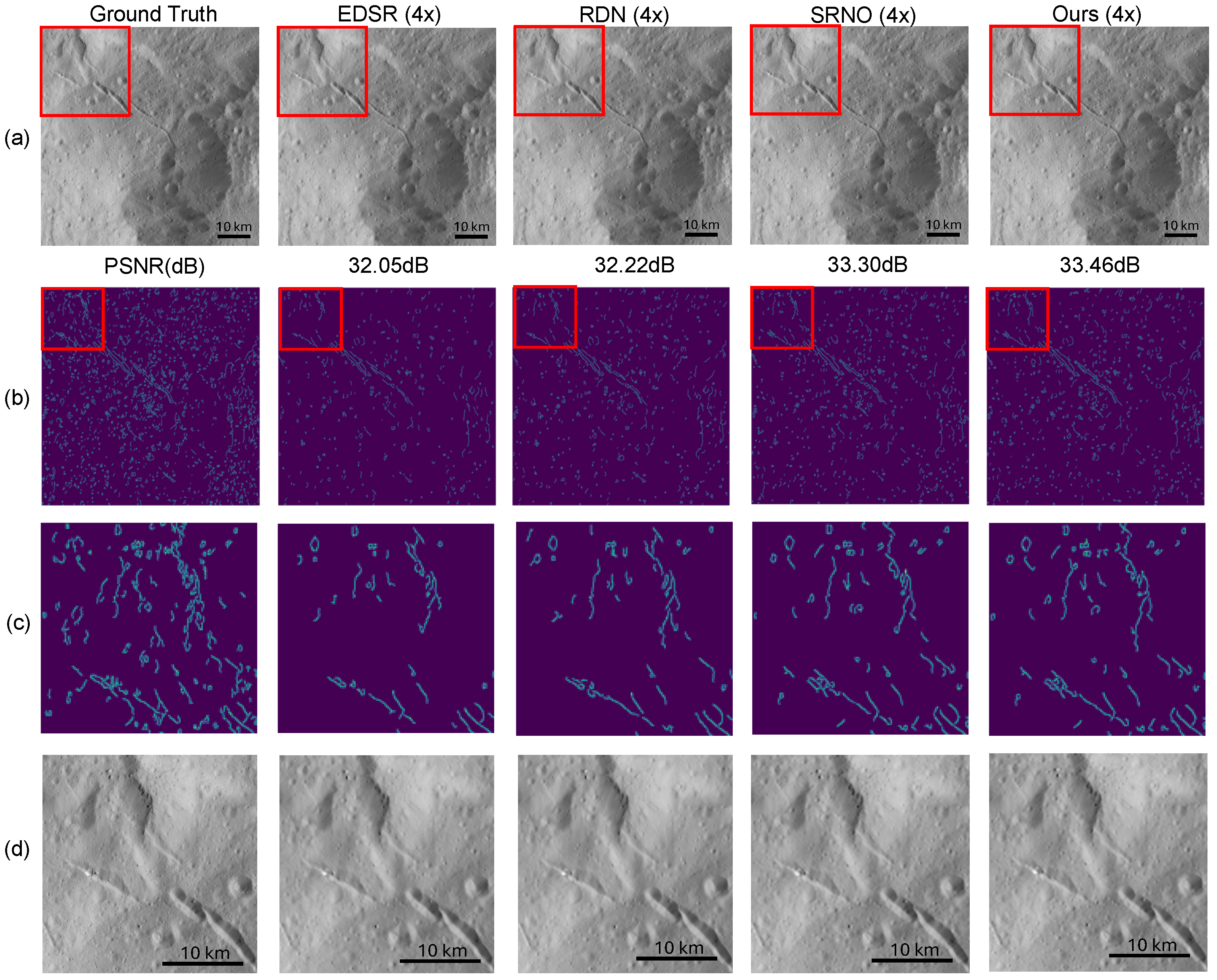
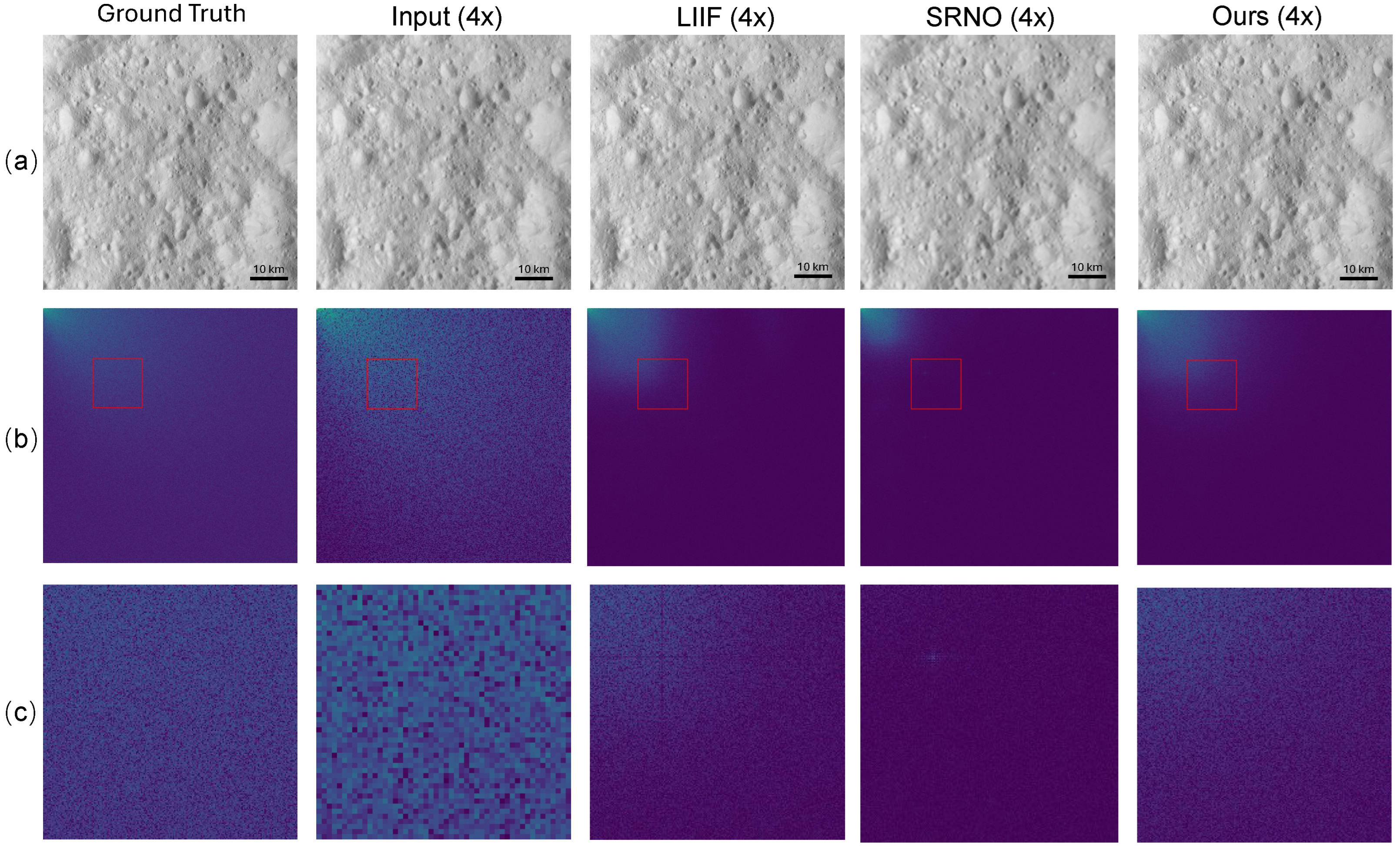
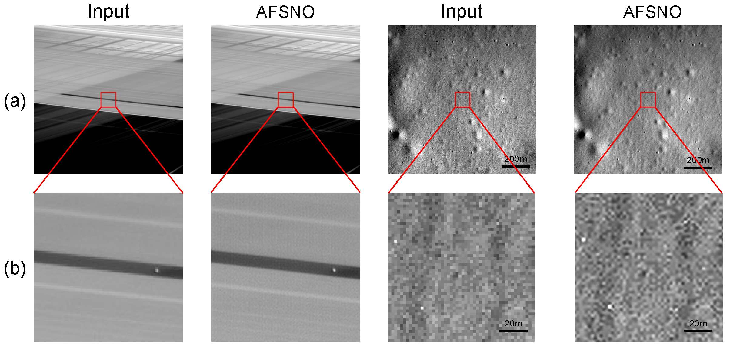
Figure 10 presents the visual results of both ground truth and SR at a 4× scale. AFSNO achieves impressive reconstruction results across various geological features on different planets. Figure 11 demonstrates the visual results of both SR and edge extraction applied to Ceres-1K at a 4× scale. The reconstructed images exhibit fine textures and clear edges for these diverse geological features. Frequency domain analysis in Figure 12 further illustrates that AFSNO’s fusion neural operator effectively mitigates spectral bias while enhancing spatial consistency. The square marked region in the edge feature map and the SR image contains rich edge details and high-frequency information. SR at an arbitrary scale demonstrates superior performance compared to single-scale methods. Both AFSNO and SRNO are capable of reconstructing fine details within this area. Furthermore, AFSNO exhibits its ability to reconstruct images with higher Peak Signal-to-Noise Ratio (PSNR) using fewer parameters in small-scale SR. Figure 13 presents visual comparisons of the reconstruction effects in the crater and linear structure areas. The SR images, with scale factors ranging from 2× to 10 ×, demonstrate that AFSNO can effectively reconstruct fine details in the focus areas, even at high scale factors. Figure 14 also demonstrates that AFSNO achieves strong performance on real planetary images, which were not included in the training dataset and for which no ground truth images are available.
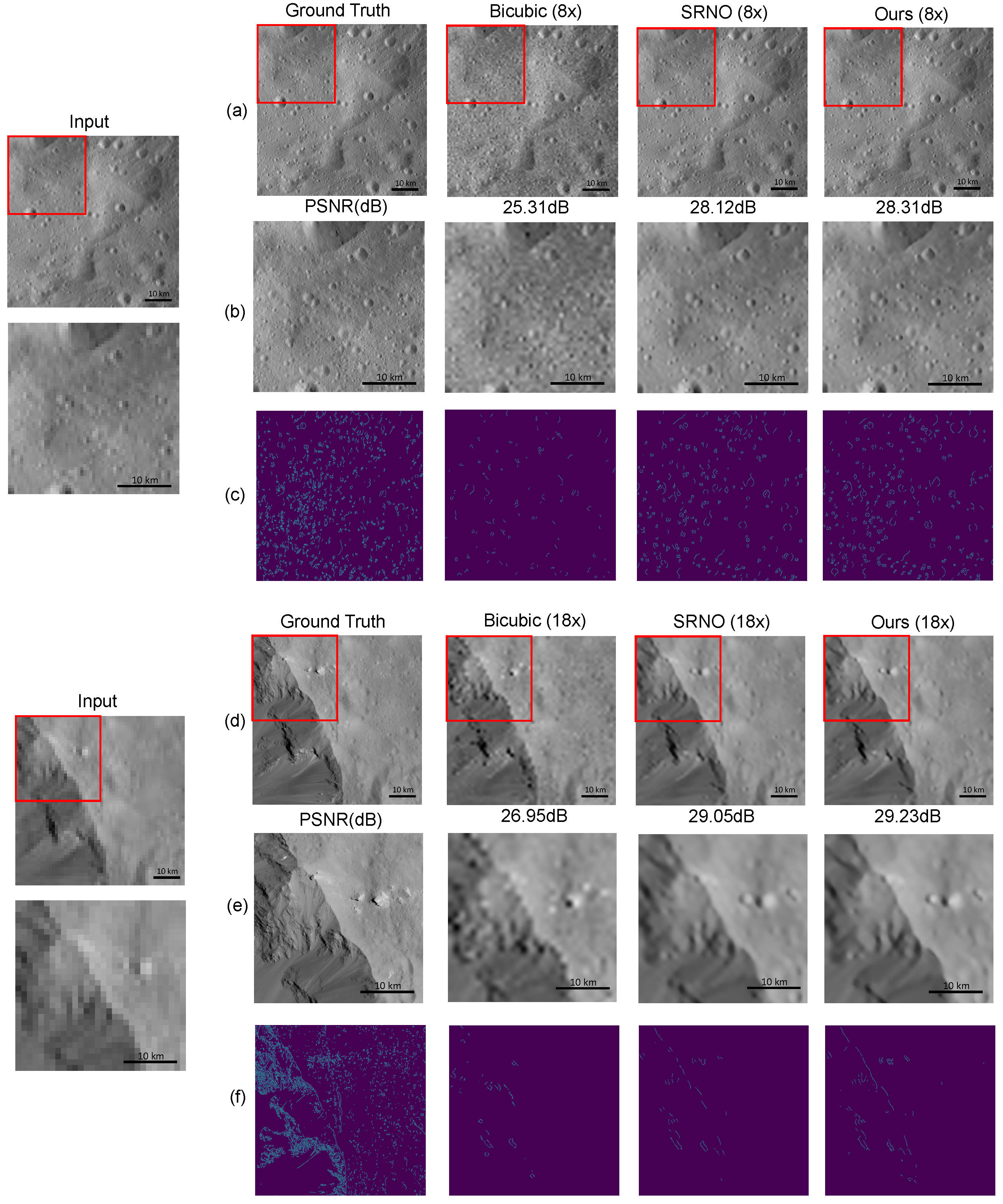
Figure 15 demonstrates the visual results of both SR and edge extraction applied to Ceres-1K in 8× scale and 18× scale. In the context of extremely high-scale SR, the image quality produced by Bicubic interpolation is unacceptable. Bicubic interpolation also introduces numerous blocky artifacts and significant block noise in the edge feature map. It is evident that AFSNO still can reconstruct more edge details in the edge feature map while maintaining a SR image that is acceptable in terms of human perception. Compared to SRNO, AFSNO maintains sharper edge reconstruction, and its edge feature map indicates better edge information reconstruction. Enhanced edge reconstruction also holds significant implications for research in Planetary Topography.

4.3. Evaluation of Unsupervised SR on Bright Spots of Ceres

The Occator Crater on Ceres hosts high-albedo faculae such as Cerealia Facula. To assess generalization without task-specific finetuning, we apply our model trained on the Ceres-1K dataset directly to bright-spot imagery. As illustrated in Figure 16, the method reconstructs sharp facula–terrain boundaries and recovers small-scale textures while suppressing blocky artifacts, indicating robust out-of-distribution performance on high-contrast targets. These results are consistent with the model’s frequency–spatial design and fusion operator, which prioritize high-frequency details and preserve edge information in regions with strong albedo gradients.

4.4. Ablation Experiment

To evaluate the contribution of each key component in our proposed AFSNO model, we conducted a systematic ablation study. We analyzed the impact of two critical components: (1) the Fusion Neural Operator (FNO) and (2) the Frequency Fusion Edge Loss (Edge). Table 4 presents quantitative results across multiple scaling factors, for both in-scale (×2, ×3, ×4) and out-of-scale (×6, ×8, ×10) SR. The Fusion Neural Operator module adds only 0.6M parameters while addressing spectral bias through adaptive frequency separation, improving PSNR by 0.03–0.07 dB across all scales, with best results at ×3 and ×4 scales where spectral bias is most challenging. The Frequency Fusion Edge Loss preserves crucial edge details in planetary geological features, yielding performance gains (0.16 dB at ×3 scale), confirming that edge preservation is essential for capturing heterogeneous terrain boundaries on planetary surfaces. The complete AFSNO model consistently outperforms all ablated variants across all scaling factors, validating our architectural design choices. Notably, while both components contribute to performance improvements, they address complementary aspects of planetary image SR: the Fusion Neural Operator improves overall reconstruction through better frequency representation, while the Edge Loss specifically enhances boundary preservation in heterogeneous regions.

4.5. Comparison Study on FSHE and EDSR-Baseline

The FSHE is an efficient, frequency–spatial neural network. Within the AFSNO framework, the LR image is mapped to a high-dimensional latent feature space using FSHE. To assess the FSHE encoder’s performance, comparative experiments were performed with both the FSHE and EDSR-baseline models, focusing on their reconstruction effect on the Ceres-1K Datasets. Both models are trained using the Adam optimizer, after removing the meanshift layer and incorporating an upsample module. The input patch sizes was fixed at 48 × 48 pixels. The experimental results are presented in Table 5 and Table 6. Additional tests were conducted to ascertain the FSHE model’s generalization ability, which included separate comparisons using bicubic and nearest downsampling conditions.
The experimental results indicate that the FSHE model outperforms the standard EDSR-baseline in terms of reconstruction quality in both nearest-neighbor and bicubic downsampling. Notably, under the nearest downsampling condition, FSHE attains a significantly higher PSNR despite having fewer parameters than EDSR-baseline. These findings underscore the enhanced efficacy of FSHE for the task of image SR.

4.6. Attribution Analysis of SRNO and AFSNO

The amount of information a model can use is a crucial metric for evaluating its performance [55]. Consequently, there is a need to analyze the region of interest for SR models. While neural networks are often perceived as inscrutable black boxes, remote sensing neural networks share similar characteristics with conventional neural networks. The recent development of the Local Attribution Map (LAM) [56] offers new insights into this domain. Based on integral gradients, LAM can elucidate the regions of interest and quantify the contribution of individual pixels in LR images for SR neural networks. In the context of remote sensing SR, the ability to utilize more information is particularly essential for enhancing model performance.
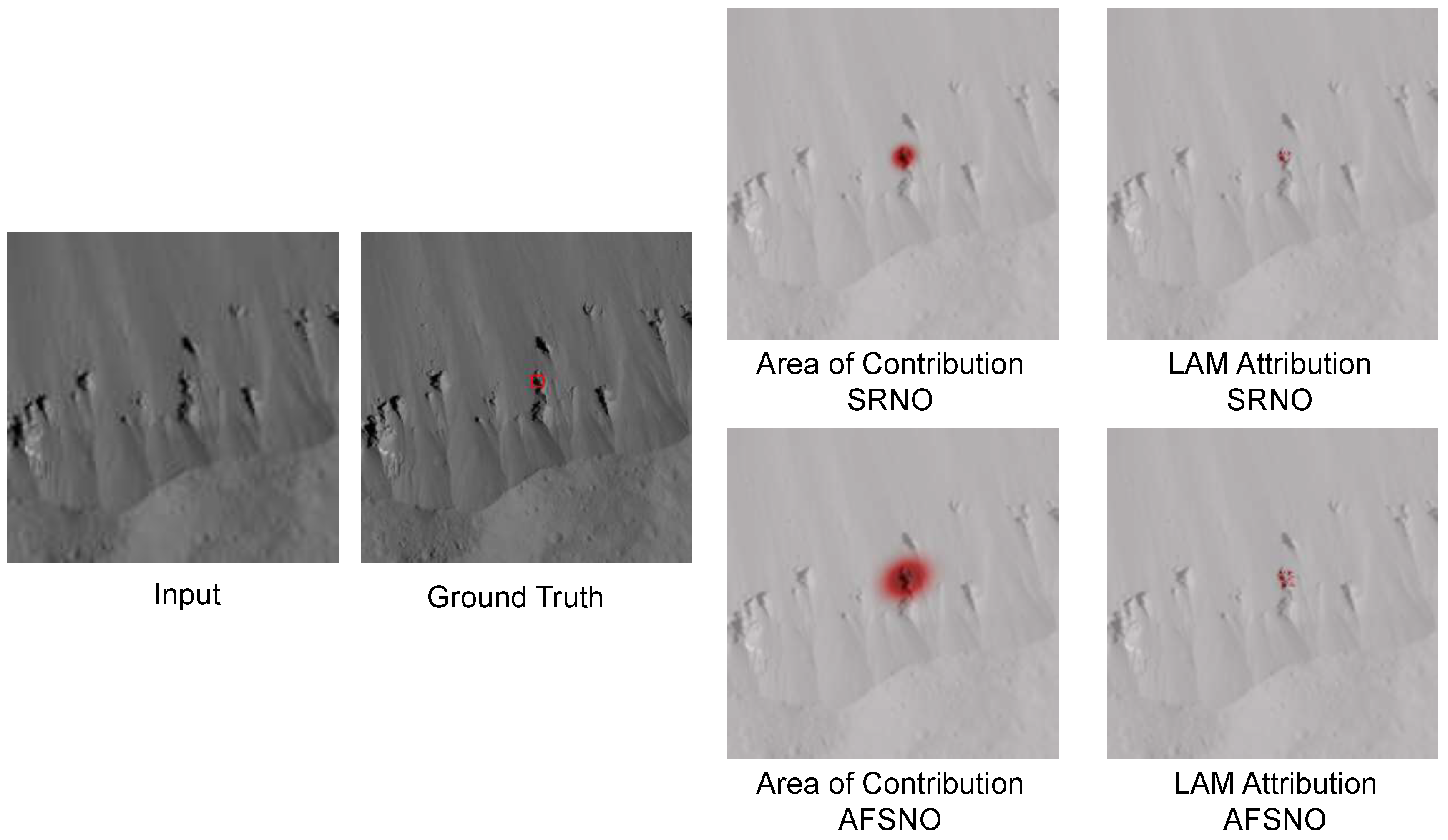
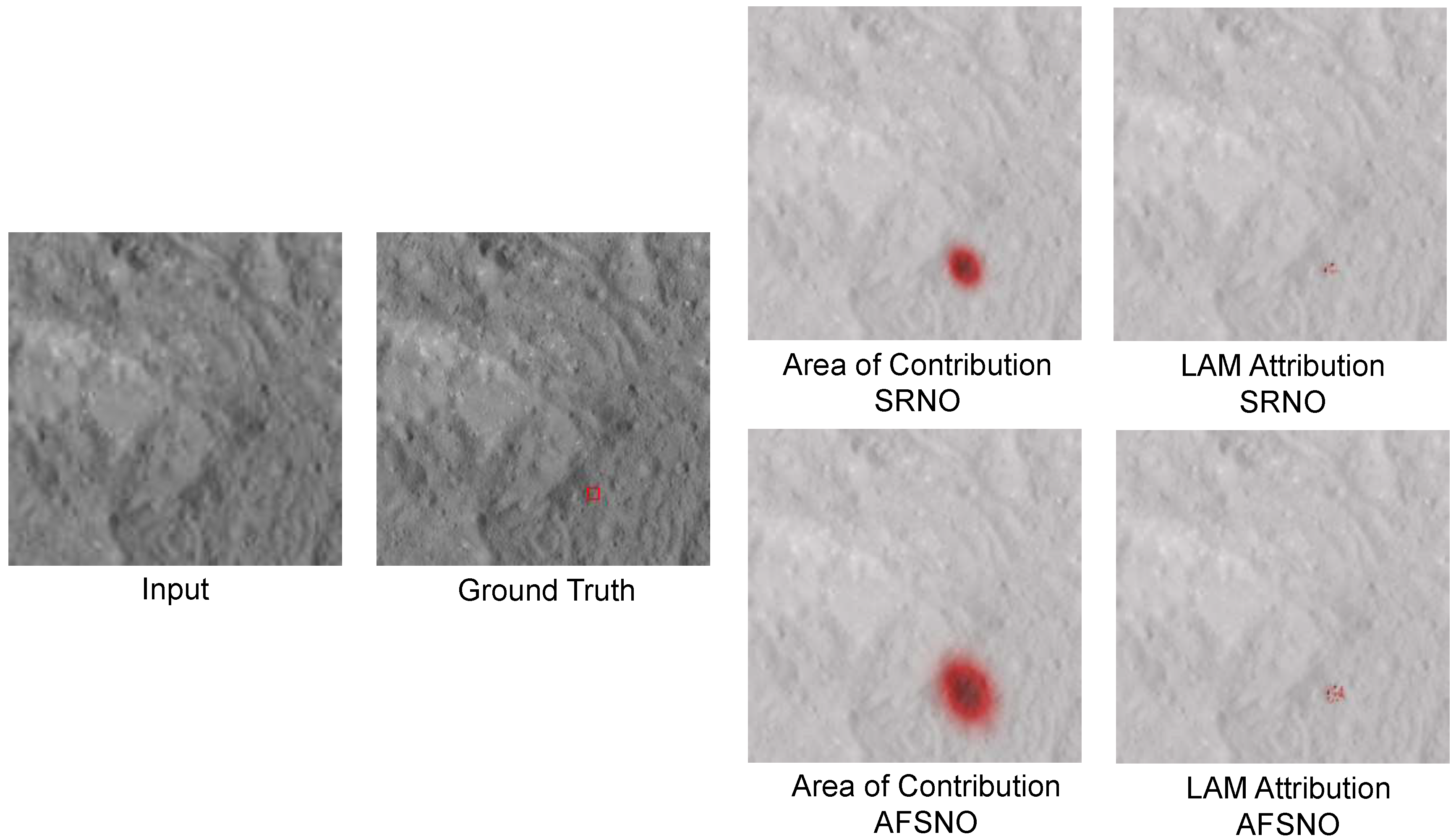
Figure 17 and Figure 18 illustrate the attribution analysis for the SRNO and the proposed AFSNO models. The contribution area represents the region utilized by the neural network to reconstruct the area marked by black boxes in the HR image. The LAM attribution indicates the contribution of each pixel. For geological features, the AFSNO achieves a larger receptive field compared to the SRNO. This suggests that the AFSNO can utilize a wider range of pixels to reconstruct the HR images [56]. Intuitively, this also indicates that the AFSNO can leverage more information to reconstruct the HR images, resulting in a strong reconstruction performance.

4.7. Generalization to Complex Planetary Remote Sensing Images

To further evaluate the AFSNO’s performance under complex imaging conditions and assess how domain variations such as lighting and noise affect model performance, we tested both AFSNO and SRNO on images degraded with an anisotropic Gaussian kernel. The anisotropic Gaussian kernel size was set to ( 4 s + 3 ) × ( 4 s + 3 ) , where s denotes the downsampling scale. The kernel width was set to [ 0.175 s , 2.5 s ] , and the rotation range was set to [ 0 , π ] . As shown in Table 7 and Table 8, AFSNO achieves competitive performance under complex degradation conditions.

4.8. Applications of AFSNO in Planetary Remote Sensing

The qualitative and quantitative results presented in Section 4.2.3 and Section 4.2.4 demonstrate that AFSNO reconstructs sharper and more continuous edges while preserving high-frequency textures across a wide range of scales, as illustrated in Figure 10, Figure 11 and Figure 12 and Figure 15. These characteristics are directly relevant to several core planetary remote sensing tasks, including crater counting and surface age estimation. Crater-size frequency distribution (CSFD) based age dating depends on consistently detecting crater rims across different scales [57,58]. The clearer and more continuous rims generated by AFSNO, as shown in Figure 12, Figure 13 and Figure 15, can reduce rim fragmentation and false merges in automated crater detection, thereby increasing confidence in manual counting. This advantage is particularly important for small craters near the resolution limit, which strongly affect the steep portion of CSFDs. By maintaining rim sharpness while mitigating spectral bias (Figure 12), AFSNO helps stabilize crater population identification across heterogeneous datasets. In terms of multi-scale data harmonization and change analysis, AFSNO allows analysts to resample images to align with existing basemaps or ancillary layers, reducing interpolation artifacts. Geomorphologic mapping and structural interpretation. Mapping of geomorphologic units and tectonic fabrics benefits from edge continuity and texture coherence. The preserved lineaments and fracture patterns (Figure 10) support delineation of structural domains and tectonic fabrics, while sharper boundaries between units improve polygon delineation in Geographic Information System workflows. The case on bright, high-albedo faculae at Occator (Section 4.3) illustrates enhanced boundary definition between reflective deposits and surrounding terrains, which is helpful for further scientific analysis.
Regarding mission operations and future onboard applications, AFSNO, with only 0.8 M parameters compared to previous arbitrary-scale SR models (Table 1), is suitable for embedded deployment scenarios. Potential applications include onboard pre-processing to generate higher-fidelity thumbnails for target selection, enhancing visual navigation. Its arbitrary-scale capability further enables adaptive magnification based on scene content or operational requirements. Moreover, AFSNO can serve as an effective pre-processing component that enhances the robustness and efficiency of planetary mapping workflows.

5. Conclusions

This work introduces AFSNO, an arbitrary-scale, lightweight planetary remote sensing super-resolution model. AFSNO addresses the characteristic of planetary remote sensing images by leveraging FSHE and a parallel frequency–spatial structure to prioritize high-frequency details that preserve fine geological features across multiple scales. AFSNO attains superior image quality with fewer parameters and reduced computational cost over scales from 2 × to 10 × . Additionally, we introduce Ceres-1K, a comprehensive planetary remote sensing dataset, filling a gap in standardized data resources for this domain. Beyond improving reconstruction fidelity, these properties support downstream planetary science tasks such as CSFD-based age estimation and structural mapping, and they align with practical constraints of future missions through a lightweight, arbitrary-scale design suitable for onboard pre-processing.
Nevertheless, AFSNO has limitations. The current implementation assumes bicubic degradation, whereas real planetary images may be affected by radiation noise, and ground-truth images may be unavailable. Future work will therefore explore AFSNO in additional SR settings, including hyperspectral image SR and unsupervised SR. Moreover, the practical use of the resulting high-resolution images requires further assessment. Subsequent studies will evaluate the model’s broader applicability and investigate downstream tasks that could benefit from its integration.

Author Contributions

All the authors made significant contributions to the study. H.-J.Z. and X.-P.L. conceived and designed global structure and methodology of the manuscript; H.-J.Z. and X.-P.L. analyzed the data and wrote the manuscript. K.-C.D. provided some valuable advice and proofread the manuscript. All authors have read and agreed to the published version of the manuscript.

Funding

This work was supported by The Science and Technology Development Fund, Macau SAR (No. 0016/2022/A1), (No. 0026/2025/RIA1) and (No. 0096/2022/A), and in part by the National Key Research and Development Program of China under grant 2022YFF0503100.

Data Availability Statement

The data presented in this study are available upon request from the corresponding author.

Conflicts of Interest

The authors declare no conflict of interest.

References

  1. Kim, J.; Lin, S.Y.; Xiao, H. Remote Sensing and Data Analyses on Planetary Topography. Remote Sens. 2023, 15, 2954. [Google Scholar] [CrossRef]
  2. Zhao, C.; Lu, Z. Remote sensing of landslides—A review. Remote Sens. 2018, 10, 279. [Google Scholar] [CrossRef]
  3. Liang, Z.; Wang, S.; Zhang, T.; Fu, Y. Blind Super-Resolution of Single Remotely Sensed Hyperspectral Image. IEEE Trans. Geosci. Remote Sens. 2023, 61, 5523314. [Google Scholar] [CrossRef]
  4. Tomczak, A.; Stępień, G.; Kogut, T.; Jedynak, Ł.; Zaniewicz, G.; Łącka, M.; Bodus-Olkowska, I. Development of a Digital Twin of the Harbour Waters and Surrounding Infrastructure Based on Spatial Data Acquired with Multimodal and Multi-Sensor Mapping Systems. Appl. Sci. 2024, 15, 315. [Google Scholar] [CrossRef]
  5. Vijayalakshmi, M.; Sasithradevi, A.; Muthuvel, P. NodYOLO-GAM: A Hybrid Multi-Scale Attention-Enhanced Convolutional Neural Network for Real-Time Polymetallic Nodule Detection in Oceanic Environments. Signal Image Video Process. 2025, 19, 1098. [Google Scholar] [CrossRef]
  6. Hao, Y.; Yan, S.; Yang, G.; Luo, Y.; Liu, D.; Han, C.; Ren, X.; Du, D. Image segmentation and coverage estimation of deep-sea polymetallic nodules based on lightweight deep learning model. Sci. Rep. 2025, 15, 10177. [Google Scholar] [CrossRef]
  7. Tomczak, A.; Kogut, T.; Kabała, K.; Abramowski, T.; Ciążela, J.; Giza, A. Automated estimation of offshore polymetallic nodule abundance based on seafloor imagery using deep learning. Sci. Total Environ. 2024, 956, 177225. [Google Scholar] [CrossRef]
  8. Dian, R.; Shan, T.; He, W.; Liu, H. Spectral super-resolution via model-guided cross-fusion network. IEEE Trans. Neural Netw. Learn. Syst. 2023, 35, 10059–10070. [Google Scholar] [CrossRef]
  9. Dian, R.; Liu, Y.; Li, S. Hyperspectral image fusion via a novel generalized tensor nuclear norm regularization. IEEE Trans. Neural Netw. Learn. Syst. 2024, 36, 7437–7448. [Google Scholar] [CrossRef]
  10. Dian, R.; Li, S. Hyperspectral image super-resolution via subspace-based low tensor multi-rank regularization. IEEE Trans. Image Process. 2019, 28, 5135–5146. [Google Scholar] [CrossRef]
  11. Dian, R.; Li, S.; Fang, L.; Bioucas-Dias, J. Hyperspectral image super-resolution via local low-rank and sparse representations. In Proceedings of the IGARSS 2018–2018 IEEE International Geoscience and Remote Sensing Symposium, Valencia, Spain, 22–27 July 2018; pp. 4003–4006. [Google Scholar]
  12. Russell, C.; Raymond, C.; Ammannito, E.; Buczkowski, D.; De Sanctis, M.C.; Hiesinger, H.; Jaumann, R.; Konopliv, A.; McSween, H.; Nathues, A.; et al. Dawn arrives at Ceres: Exploration of a small, volatile-rich world. Science 2016, 353, 1008–1010. [Google Scholar] [CrossRef]
  13. Buczkowski, D.; Schmidt, B.E.; Williams, D.; Mest, S.; Scully, J.; Ermakov, A.; Preusker, F.; Schenk, P.; Otto, K.A.; Hiesinger, H.; et al. The geomorphology of Ceres. Science 2016, 353, aaf4332. [Google Scholar] [CrossRef]
  14. Sierks, H.; Keller, H.; Jaumann, R.; Michalik, H.; Behnke, T.; Bubenhagen, F.; Büttner, I.; Carsenty, U.; Christensen, U.; Enge, R.; et al. The Dawn framing camera. Space Sci. Rev. 2011, 163, 263–327. [Google Scholar] [CrossRef]
  15. Timofte, R.; Gu, S.; Wu, J.; Van Gool, L.; Zhang, L.; Yang, M.H.; Haris, M.; Shakhnarovich, G.; Ukita, N.; Hu, S.; et al. NTIRE 2018 Challenge on Single Image Super-Resolution: Methods and Results. In Proceedings of the IEEE Conference on Computer Vision and Pattern Recognition (CVPR) Workshops, Salt Lake City, UT, USA, 18–23 June 2018. [Google Scholar] [CrossRef]
  16. Lim, B.; Son, S.; Kim, H.; Nah, S.; Mu Lee, K. Enhanced deep residual networks for single image super-resolution. In Proceedings of the IEEE Conference on Computer Vision and Pattern Recognition Workshops, Honolulu, HI, USA, 21–26 July 2017; pp. 136–144. [Google Scholar] [CrossRef]
  17. Niu, B.; Wen, W.; Ren, W.; Zhang, X.; Yang, L.; Wang, S.; Zhang, K.; Cao, X.; Shen, H. Single image super-resolution via a holistic attention network. In Proceedings of the Computer Vision–ECCV 2020: 16th European Conference, Glasgow, UK, 23–28 August 2020; Part XII 16. pp. 191–207. [Google Scholar]
  18. Liang, J.; Cao, J.; Sun, G.; Zhang, K.; Van Gool, L.; Timofte, R. Swinir: Image restoration using swin transformer. In Proceedings of the IEEE/CVF International Conference on Computer Vision, Montreal, BC, Canada, 11–17 October 2021; pp. 1833–1844. [Google Scholar] [CrossRef]
  19. Dong, C.; Loy, C.C.; He, K.; Tang, X. Image super-resolution using deep convolutional networks. IEEE Trans. Pattern Anal. Mach. Intell. 2015, 38, 295–307. [Google Scholar] [CrossRef]
  20. Chen, Y.; Liu, S.; Wang, X. Learning continuous image representation with local implicit image function. In Proceedings of the IEEE/CVF Conference on Computer Vision and Pattern Recognition, Nashville, TN, USA, 20–25 June 2021; pp. 8628–8638. [Google Scholar] [CrossRef]
  21. Lee, J.; Jin, K.H. Local texture estimator for implicit representation function. In Proceedings of the IEEE/CVF Conference on Computer Vision and Pattern Recognition, New Orleans, LA, USA, 18–24 June 2022; pp. 1929–1938. [Google Scholar] [CrossRef]
  22. Wei, M.; Zhang, X. Super-Resolution Neural Operator. In Proceedings of the IEEE/CVF Conference on Computer Vision and Pattern Recognition (CVPR), Vancouver, BC, Canada, 17–24 June 2023; pp. 18247–18256. [Google Scholar] [CrossRef]
  23. Wu, H.; Ni, N.; Zhang, L. Learning dynamic scale awareness and global implicit functions for continuous-scale super-resolution of remote sensing images. IEEE Trans. Geosci. Remote Sens. 2023, 61, 1–15. [Google Scholar] [CrossRef]
  24. Galar, M.; Sesma, R.; Ayala, C.; Albizua, L.; Aranda, C. Super-resolution of sentinel-2 images using convolutional neural networks and real ground truth data. Remote Sens. 2020, 12, 2941. [Google Scholar] [CrossRef]
  25. Salgueiro Romero, L.; Marcello, J.; Vilaplana, V. Super-resolution of sentinel-2 imagery using generative adversarial networks. Remote Sens. 2020, 12, 2424. [Google Scholar] [CrossRef]
  26. Rahaman, N.; Baratin, A.; Arpit, D.; Draxler, F.; Lin, M.; Hamprecht, F.; Bengio, Y.; Courville, A. On the spectral bias of neural networks. In Proceedings of the International Conference on Machine Learning, PMLR, Long Beach, CA, USA, 9–15 June 2019; pp. 5301–5310. [Google Scholar]
  27. Li, H.; Dai, T.; Li, Y.; Zou, X.; Xia, S.T. Adaptive local implicit image function for arbitrary-scale super-resolution. In Proceedings of the 2022 IEEE International Conference on Image Processing (ICIP), Bordeaux, France, 16–19 October 2022; pp. 4033–4037. [Google Scholar] [CrossRef]
  28. Zhang, T.; Bian, C.; Zhang, X.; Chen, H.; Chen, S. Lightweight remote-sensing image super-resolution via re-parameterized feature distillation network. IEEE Geosci. Remote Sens. Lett. 2023, 20, 1–5. [Google Scholar] [CrossRef]
  29. Mei, S.; Jiang, R.; Li, X.; Du, Q. Spatial and spectral joint super-resolution using convolutional neural network. IEEE Trans. Geosci. Remote Sens. 2020, 58, 4590–4603. [Google Scholar] [CrossRef]
  30. Zhang, H.; Wang, P.; Jiang, Z. Nonpairwise-trained cycle convolutional neural network for single remote sensing image super-resolution. IEEE Trans. Geosci. Remote Sens. 2020, 59, 4250–4261. [Google Scholar] [CrossRef]
  31. Xie, S.; Girshick, R.; Dollár, P.; Tu, Z.; He, K. Aggregated residual transformations for deep neural networks. In Proceedings of the IEEE Conference on Computer Vision and Pattern Recognition, Honolulu, HI, USA, 21–26 July 2017; pp. 1492–1500. [Google Scholar]
  32. Zhang, Y.; Li, K.; Li, K.; Wang, L.; Zhong, B.; Fu, Y. Image super-resolution using very deep residual channel attention networks. In Proceedings of the European Conference on Computer Vision (ECCV), Munich, Germany, 8–14 September 2018; pp. 286–301. [Google Scholar]
  33. Zhang, Y.; Tian, Y.; Kong, Y.; Zhong, B.; Fu, Y. Residual dense network for image super-resolution. In Proceedings of the IEEE Conference on Computer Vision and Pattern Recognition, Salt Lake City, UT, USA, 18–23 June 2018; pp. 2472–2481. [Google Scholar] [CrossRef]
  34. Ma, W.; Pan, Z.; Yuan, F.; Lei, B. Super-resolution of remote sensing images via a dense residual generative adversarial network. Remote Sens. 2019, 11, 2578. [Google Scholar] [CrossRef]
  35. Tao, Y.; Conway, S.J.; Muller, J.P.; Putri, A.R.; Thomas, N.; Cremonese, G. Single image super-resolution restoration of TGO CaSSIS colour images: Demonstration with perseverance rover landing site and Mars science targets. Remote Sens. 2021, 13, 1777. [Google Scholar] [CrossRef]
  36. Chen, K.; Li, W.; Lei, S.; Chen, J.; Jiang, X.; Zou, Z.; Shi, Z. Continuous remote sensing image super-resolution based on context interaction in implicit function space. IEEE Trans. Geosci. Remote Sens. 2023, 61, 1–16. [Google Scholar] [CrossRef]
  37. Mao, X.; Liu, Y.; Liu, F.; Li, Q.; Shen, W.; Wang, Y. Intriguing findings of frequency selection for image deblurring. In Proceedings of the AAAI Conference on Artificial Intelligence, Washington, DC, USA, 7–14 February 2023; Volume 37, pp. 1905–1913. [Google Scholar] [CrossRef]
  38. Zhao, Z.; Zhang, J.; Xu, S.; Lin, Z.; Pfister, H. Discrete cosine transform network for guided depth map super-resolution. In Proceedings of the IEEE/CVF Conference on Computer Vision and Pattern Recognition, New Orleans, LA, USA, 18–24 June 2022; pp. 5697–5707. [Google Scholar] [CrossRef]
  39. Guo, T.; Mousavi, H.S.; Monga, V. Adaptive transform domain image super-resolution via orthogonally regularized deep networks. IEEE Trans. Image Process. 2019, 28, 4685–4700. [Google Scholar] [CrossRef]
  40. Shi, W.; Caballero, J.; Huszár, F.; Totz, J.; Aitken, A.P.; Bishop, R.; Rueckert, D.; Wang, Z. Real-time single image and video super-resolution using an efficient sub-pixel convolutional neural network. In Proceedings of the IEEE Conference on Computer Vision and Pattern Recognition, Las Vegas, NV, USA, 27–30 June 2016; pp. 1874–1883. [Google Scholar] [CrossRef]
  41. Li, J.; Fang, F.; Mei, K.; Zhang, G. Multi-scale residual network for image super-resolution. In Proceedings of the European Conference on Computer Vision (ECCV), Munich, Germany, 8–14 September 2018; pp. 517–532. [Google Scholar]
  42. Kim, J.; Lee, J.K.; Lee, K.M. Accurate image super-resolution using very deep convolutional networks. In Proceedings of the IEEE Conference on Computer Vision and Pattern Recognition, Las Vegas, NV, USA, 27–30 June 2016; pp. 1646–1654. [Google Scholar]
  43. Yang, F.; Yang, H.; Fu, J.; Lu, H.; Guo, B. Learning texture transformer network for image super-resolution. In Proceedings of the IEEE/CVF Conference on Computer Vision and Pattern Recognition, Seattle, WA, USA, 13–19 June 2020; pp. 5791–5800. [Google Scholar] [CrossRef]
  44. Ramunno, F.P.; Massa, P.; Kinakh, V.; Panos, B.; Csillaghy, A.; Voloshynovskiy, S. Enhancing image resolution of solar magnetograms: A latent diffusion model approach. Astron. Astrophys. 2025, 698, A140. [Google Scholar] [CrossRef]
  45. Chen, X.; Wang, X.; Zhou, J.; Qiao, Y.; Dong, C. Activating more pixels in image super-resolution transformer. In Proceedings of the IEEE/CVF Conference on Computer Vision and Pattern Recognition, Vancouver, BC, Canada, 17–24 June 2023; pp. 22367–22377. [Google Scholar] [CrossRef]
  46. Hu, X.; Mu, H.; Zhang, X.; Wang, Z.; Tan, T.; Sun, J. Meta-SR: A magnification-arbitrary network for super-resolution. In Proceedings of the IEEE/CVF Conference on Computer Vision and Pattern Recognition, Long Beach, CA, USA, 15–20 June 2019; pp. 1575–1584. [Google Scholar] [CrossRef]
  47. Tancik, M.; Srinivasan, P.; Mildenhall, B.; Fridovich-Keil, S.; Raghavan, N.; Singhal, U.; Ramamoorthi, R.; Barron, J.; Ng, R. Fourier features let networks learn high frequency functions in low dimensional domains. Adv. Neural Inf. Process. Syst. 2020, 33, 7537–7547. [Google Scholar]
  48. Howard, A.G.; Zhu, M.; Chen, B.; Kalenichenko, D.; Wang, W.; Weyand, T.; Andreetto, M.; Adam, H. Mobilenets: Efficient convolutional neural networks for mobile vision applications. arXiv 2017, arXiv:1704.04861. [Google Scholar] [CrossRef]
  49. Chollet, F. Xception: Deep learning with depthwise separable convolutions. In Proceedings of the IEEE Conference on Computer Vision and Pattern Recognition, Honolulu, HI, USA, 21–26 July 2017; pp. 1251–1258. [Google Scholar]
  50. Chen, J.; He, T.; Zhuo, W.; Ma, L.; Ha, S.; Chan, S.H.G. Tvconv: Efficient translation variant convolution for layout-aware visual processing. In Proceedings of the IEEE/CVF Conference on Computer Vision and Pattern Recognition, New Orleans, LA, USA, 18–24 June 2022; pp. 12548–12558. [Google Scholar] [CrossRef]
  51. Li, J.; Wen, Y.; He, L. SCConv: Spatial and Channel Reconstruction Convolution for Feature Redundancy. In Proceedings of the IEEE/CVF Conference on Computer Vision and Pattern Recognition, Vancouver, BC, Canada, 17–24 June 2023; pp. 6153–6162. [Google Scholar] [CrossRef]
  52. Moser, B.B.; Raue, F.; Frolov, S.; Palacio, S.; Hees, J.; Dengel, A. Hitchhiker’s Guide to Super-Resolution: Introduction and Recent Advances. IEEE Trans. Pattern Anal. Mach. Intell. 2023, 45, 9862–9882. [Google Scholar] [CrossRef]
  53. Ern, A.; Guermond, J.L. Theory and Practice of Finite Elements; Springer: New York, NY, USA, 2004; Volume 159. [Google Scholar]
  54. Kumar, N.; Verma, R.; Sethi, A. Convolutional neural networks for wavelet domain super resolution. Pattern Recognit. Lett. 2017, 90, 65–71. [Google Scholar] [CrossRef]
  55. Wang, J.; Wang, B.; Wang, X.; Zhao, Y.; Long, T. Hybrid attention based u-shaped network for remote sensing image super-resolution. IEEE Trans. Geosci. Remote Sens. 2023, 61, 5612515. [Google Scholar] [CrossRef]
  56. Gu, J.; Dong, C. Interpreting super-resolution networks with local attribution maps. In Proceedings of the IEEE/CVF Conference on Computer Vision and Pattern Recognition, Nashville, TN, USA, 20–25 June 2021; pp. 9199–9208. [Google Scholar] [CrossRef]
  57. Barlow, N.G. Crater size-frequency distributions and a revised Martian relative chronology. Icarus 1988, 75, 285–305. [Google Scholar] [CrossRef]
  58. Michael, G.; Neukum, G. Planetary surface dating from crater size–frequency distribution measurements: Partial resurfacing events and statistical age uncertainty. Earth Planet. Sci. Lett. 2010, 294, 223–229. [Google Scholar] [CrossRef]
Figure 1. Examples of Ceres images (a) and natural images (b), demonstrating their different context distributions. These context distinct distributions necessitate domain-specific feature learning mechanisms, as generic natural image priors in natural images may degrade SR performance on planetary remote sensing images.
Remotesensing 17 03718 g001
Figure 2. The t-SNE visualization of image patches from Ceres-1K and widely used natural image datasets. Each scatter plot represents the t-SNE visualization of patches from a randomly selected image. The analysis demonstrates higher regional context homogeneity in Ceres-1K patches compared to natural image patches, quantifying the distinct contextual characteristics of planetary remote sensing images.
Remotesensing 17 03718 g002
Figure 3. Architecture of the Adaptive Frequency–Spatial Neural Operator (AFSNO).
Remotesensing 17 03718 g003
Figure 4. The architecture of ESRU. The ESCB consists of the CRU and ESRU.
Remotesensing 17 03718 g004
Figure 5. The architecture of Fusion Neural Operator.
Remotesensing 17 03718 g005
Figure 6. The architecture of Galerkin-Type Attention.
Remotesensing 17 03718 g006
Figure 7. The architecture of the Frequency Split Block (FSB) and the Frequency Concatenate Block (FCB). These two blocks are designed to separate frequency domain features into high-frequency and low-frequency components by cropping the features. Panels (ad) illustrate the different frequency information extracted through the frequency split operation.
Remotesensing 17 03718 g007
Figure 8. Visualization of features used in the Frequency Fusion Edge Loss function. Input-Laplace represents input images after applying the Laplace edge operator. The DWT decomposes the input planetary remote sensing image into four subbands: Input-DWT-LL, Input-DWT-HL, Input-DWT-LH, and Input-DWT-HH, all components of the Frequency Fusion Edge Loss Function.
Remotesensing 17 03718 g008
Figure 9. Examples from the Ceres-1K dataset. The Ceres-1K dataset exhibits rich geological features, such as craters, linear structures, mounds, and domes.
Remotesensing 17 03718 g009
Figure 10. Qualitative comparison of 4× SR results for different geological features on various planets. (a) Central mound at the south pole on Vesta. (b) Charon’s complexity. (c) Detailed ‘Snowman’ Crater on Vesta. (d) Detailed ’Snowman’ crater on Vesta. (e) Northern hemisphere of Triton, the moon of Neptune. (f) Old and heavily cratered terrain on Vesta. (gl) Different morphologic features on Ceres. Linear structures are denoted by arrows in (i). Small mound denoted by arrows in (k). The planetary remote sensing images (fl) were acquired by the framing camera on the Dawn orbiter. The images (af) were not included in the training dataset.
Remotesensing 17 03718 g010
Figure 11. Qualitative comparison in 4× SR, where the image depicts the surface of the Ceres. Group (a) denotes the ground truth, input image and SR images. Group (b) denotes the image’s edge feature map extracted by the Canny edge detector. Group (c) denotes the selected area of the image’s edge feature map are detected by the Canny edge detector. Group (d) denotes the select area of the ground truth, input image and SR images. Those images were not included in the training dataset. This edge preservation is essential for crater counting and unit boundary delineation on Ceres. These images were not included in the training dataset. The planetary remote sensing image is acquired by the framing camera on the Dawn orbiter.
Remotesensing 17 03718 g011
Figure 12. Visual comparisons of 4× SR in both spatial and frequency domains are presented, where the image depicts the surface of the Ceres. (a) denotes the planetary remote sensing images, (b) shows the frequency domain generated by DCT, and (c) presents the selected areas of the images’s frequency domain. The results demonstrate that AFSNO reduces spectral bias relative to baselines while improving spatial coherence, consistent with its frequency–spatial fusion design. The planetary remote sensing image is acquired by the framing camera on the Dawn orbiter.
Remotesensing 17 03718 g012
Figure 13. Visual comparisons of crater images from the southern hemisphere of dwarf planet Ceres from an altitude of 1470 km with different scale factors ranging from 2× to 10×. AFSNO maintains rim integrity and intra-crater texture as magnification increases, indicating robust reconstruction of high-frequency content needed for crater size-frequency distribution (CSFD) analyses. The planetary remote sensing image is acquired by the framing camera on the Dawn orbiter.
Remotesensing 17 03718 g013
Figure 14. Qualitative comparison of 4 × SR results for real images from various planets. The (a) denotes planetary remote sensing images. The (b) denotes selected regions from the planetary remote sensing images.The image on the left depicts Saturn’s criss-crossed rings, and the one on the right shows the surface of Mercury. Those images were not included in the training dataset and for which no ground truth images are available.
Remotesensing 17 03718 g014
Figure 15. Qualitative comparison of 8× and 18× SR results. Group (a) denotes the ground truth and SR images in 8× SR. Group (b) denotes the marked area of the ground truth and SR images in 8× SR. Group (c) denotes the image’s edge feature map extracted by the Canny operator in 8× SR. Group (d) denotes the ground truth and SR images in 18× SR. Group (e) denotes the selected area of the ground truth and SR images in 18× SR. Group (f) denotes the image’s edge feature map extracted by the Canny operator in 18× SR. The planetary remote sensing image is acquired by the framing camera on the Dawn orbiter.
Remotesensing 17 03718 g015
Figure 16. Visual results for 4× SR on bright-spot images of Ceres using a model trained exclusively on Ceres-1K. These bright spots may be related to a type of salt. These images were not included in the training dataset.
Remotesensing 17 03718 g016
Figure 17. Attribution results of SRNO and AFSNO in rugged area of Ceres.
Remotesensing 17 03718 g017
Figure 18. Attribution results of SRNO and AFSNO in flat area of Ceres.
Remotesensing 17 03718 g018
Table 1. Average Peak Signal-to-Noise Ratio (PSNR) on the CERES-1K test set. The best results are emphasized with bold.
Method×2×3×4×6×8×10 Params.
EDSR-baseline     36.68  32.61  31.401.2 M
RDN36.8632.7331.532.2 M
HAN36.8432.6631.4715.9 M
SwinIR36.9434.0532.3611.8 M
Meta-SR    36.79   34.07    32.43   30.47    29.30   28.49   1.7 M
LIIF37.1534.2132.4930.4929.3128.511.6 M
ALIIF37.1834.2232.4930.4929.3128.502.1 M
LTE37.2334.2632.5230.5129.3328.511.7 M
SRNO37.3134.3332.6130.5829.3828.572.0 M
AFSNO37.4534.4932.7330.6929.4828.650.8 M
Table 2. Average Structural Similarity Index (SSIM) on the CERES-1K test set. The best results are emphasized with bold.
Method×2×3×4×6×8×10 Params.
EDSR-baseline   0.9110.7930.7311.2 M
RDN0.9150.7960.7362.2 M
HAN0.9140.8120.77115.9 M
SwinIR0.9240.8570.78911.8 M
Meta-SR    0.931   0.868    0.804   0.702    0.637   0.596   1.7 M
LIIF0.9280.8610.7960.6950.6310.5911.6 M
ALIIF0.9280.8610.7960.6940.6310.5922.1 M
LTE0.9290.8620.7960.6940.6310.5911.7 M
SRNO0.9300.8630.7990.6970.6330.5932.0 M
AFSNO0.9320.8670.8040.7030.6390.5990.8 M
Table 3. Comparison of model efficiency in FLOPs. The best results are emphasized with bold.
MethodFLOPs (G)
LIIF12.24
ALIIF12.02
LTE16.98
SRNO9.25
AFSNO (ours)3.70
Table 4. Ablation study of AFSNO on PSNR (dB). FNO denotes the Fusion Neural Operator component, and Edge denotes the Frequency Fusion Edge Loss. The best results are emphasized with bold.
Method×2×3×4×6×8×10 Params.
AFSNO(-FNO)(-EDGE)   37.37 34.32 32.62 30.59 29.40  28.590.2 M
AFSNO(-FNO)37.3834.3332.6530.6129.4128.590.2 M
AFSNO(-EDGE)37.4234.4732.7230.6829.4728.640.8 M
AFSNO37.4534.4932.7330.6929.4828.650.8 M
Table 5. Comparison of the PSNR and the model parameters of the EDSR-baseline and FSHE in nearest downsample. The best results are emphasized with bold.
Method×2×3×4Params.
EDSR-baseline35.2829.8629.371.2 M
FSHE35.4430.4529.860.3 M
Table 6. Comparison of the PSNR and the Model Parameters of the EDSR-Baseline and FSHE in Bicubic downsample. The best results are emphasized with bold.
Method×2×3×4Params.
EDSR-baseline36.6832.6131.401.2 M
FSHE36.7532.6231.420.3 M
Table 7. Average PSNR on the Ceres-1K test set using the Anisotropic Gaussian Kernel for degradation. The best results are emphasized with bold.
Method×2×3×4×6×8×10Params.
SRNO34.7931.9229.4727.2825.9324.862.0 M
AFSNO34.9731.9729.5327.4126.1425.160.8 M
Table 8. Average SSIM on the Ceres-1K test set using the Anisotropic Gaussian Kernel for degradation. The best results are emphasized with bold.
Method×2×3×4×6×8×10Params.
SRNO0.8900.8030.6900.5790.5240.4932.0 M
AFSNO0.8910.8060.6910.5820.5290.4980.8 M
Disclaimer/Publisher’s Note: The statements, opinions and data contained in all publications are solely those of the individual author(s) and contributor(s) and not of MDPI and/or the editor(s). MDPI and/or the editor(s) disclaim responsibility for any injury to people or property resulting from any ideas, methods, instructions or products referred to in the content.