Highlights
What are the main findings?
- A Dual-path U-Net is proposed for weather radar synthesis.
- This Unet can automatically remove noise from visible-light observations.
- An illumination-aware classification network is fused with weather radar synthesis.
What is the implication of the main finding?
- The automatic noise removal feature improves the accuracy of weather radar synthesis.
- The fusion of an illumination-aware classification network provides a better solution for weather radar synthesis under different lighting conditions.
Abstract
Weather radar reflectivity plays a critical role in precipitation estimation and convective storm identification. However, due to terrain limitations and the uneven spatial distribution of radar stations, oceanic regions have long suffered from a lack of radar observations, resulting in extensive monitoring gaps. Geostationary meteorological satellites have wide-area coverage and near-real-time observation capability, offering a viable solution for synthesizing radar reflectivity in these regions. Most previous synthesis studies have adopted fixed time-window data partitioning, which introduces significant noise into visible-light observations under large-scale, low-illumination conditions, thereby degrading synthesis quality. To address this issue, we propose an integrated deep-learning method that combines illumination-based classification and reflectivity synthesis to enhance the accuracy of radar reflectivity synthesis from geostationary meteorological satellites. This approach integrates a classification network with a synthesis network. First, visible-light observations from the Himawari-8 satellite are classified based on illumination conditions to separate valid signals from noise; then, noise-free infrared observations and multimodal fused data are fed into dedicated synthesis networks to generate composite reflectivity products. In experiments, the proposed method outperformed the baseline approach in regions with strong convection (≥35 dBZ), with a 9.5% improvement in the critical success index, a 7.5% increase in the probability of detection, and a 6.1% reduction in the false alarm rate. Additional experiments confirmed the applicability and robustness of the method across various complex scenarios.
1. Introduction
Severe convective weather is destructive and unpredictable, and poses significant challenges in meteorological monitoring and forecasting [1]. Meteorologists rely on weather radar as a primary monitoring tool to mitigate the adverse effects of severe conductive weather on human activities and infrastructure [2]. The effectiveness of weather radar in this role is largely attributed to its exceptionally high spatial and temporal resolution [3], allowing meteorologists to track and forecast severe convective weather in real time simply by analyzing radar echo data. Weather radar captures cloud and precipitation information through reflectivity echoes, enabling the visualization of precipitation distribution and intensity, which can be used to identify further characteristics of severe convective weather [4]. The radar echo intensity is a key indicator of convective activity in different regions, with reflectivity values ≥35 dBZ commonly interpreted as heavy precipitation [5].
Sparsely distributed ground-based radar stations can be complemented by geostationary satellites. Recent advances in satellite technology have expanded the availability of meteorological datasets, providing broader spatial coverage and multispectral observations. Although satellites provide broader spatial coverage and multispectral information, their observations focus primarily on the upper parts of cloud systems, making it difficult to capture directly convective structures beneath clouds. Additionally, while satellites can be used to monitor convective phenomena, their detection rates are limited, and false alarm rates (FARs) remain relatively high, which restricts their direct applicability in forecasting and other meteorological operations. In contrast, ground-based radar offers clearer, more accurate depictions of sub-cloud convective structures [6].
To address these limitations, researchers have explored synthetic weather radar techniques, which generate radar-like products from multi-source meteorological data in regions lacking direct radar coverage [7]. For example, the Global Synthetic Weather Radar framework integrates satellite imagery, lightning observations, and numerical weather model outputs to produce operationally relevant radar products such as composite reflectivity (CREF) [6,8,9].
Recent studies have explored mapping satellite cloud-top features to radar products to enhance the detection of severe convective weather in regions without radar coverage. For example, a machine-learning framework combining satellite infrared and passive microwave observations was proposed to estimate precipitation rates using radar-derived data as supervisory signals. While this approach improved precipitation estimation, it did not directly reconstruct CREF. In contrast, a deep-learning model based on U-Net was developed to synthesize radar CREF directly from geostationary satellite imagery, achieving high consistency with actual radar observations; however, as the model was based only on satellite data from 08:00 to 17:00 Beijing time, excluding nighttime and low-illumination samples, it did not explicitly address visible-light interference under such conditions, and its generalizability during nighttime or twilight transitions remains to be validated [10,11].
In the past decade, several emerging models have utilized satellite data to simulate and generate precipitation radar data. These models are typically implemented using traditional machine-learning methods or simple artificial neural networks (ANNs) [12]. For example, the classic Precipitation Estimation from Remotely Sensed Information using Artificial Neural Networks (PERSIANN) model employs an adaptive ANN as its primary structure, combining satellite infrared information to estimate and measure ground precipitation. However, such traditional methods suffer from low computational accuracy and often fail to deliver satisfactory synthesis results in complex meteorological environments [13].
Various artificial-intelligence methods have also been proposed for synthesizing radar data from satellite data based on deep-learning techniques. These methods have effectively addressed the low accuracy associated with traditional machine-learning models. The PERSIANN model has been expanded through the incorporation of a convolutional neural network (PERSIANN-CNN) and a stacked denoising autoencoder (PERSIANN-SDAE) [13]. These algorithms leverage deep neural networks to capture more complex physical information features compared to traditional machine-learning methods, and significantly enhance synthesis model accuracy. For example, the CNN-based Infrared Precipitation Estimation using CNN (IPEC) model significantly outperformed the PERSIANN model in terms of correlation, bias, and error metrics, although the model was error-prone under complex weather conditions due to its reliance on indirect variables such as cloud-top temperature, particularly in low-latitude convective systems [14]. The generative adversarial network-based Domain-to-Domain translation model innovatively integrated visible and infrared data from geostationary satellites, eliminating nocturnal interference from visible-light data through temporal segmentation [15]. By combining normalization and denormalization processes, the model successfully synthesized radar data from satellite observations, significantly improving precipitation estimation accuracy in radar-sparse regions. This approach highlights the importance of using visible-light data as an effective synthesis source, while minimizing nighttime interference to maximize model utility [16,17].
Although recent studies have explored CREF synthesis using multimodal satellite data, most rely on coarse temporal segmentation to differentiate between daytime and nighttime visible-light conditions. This strategy fails to account for dynamic shifts in solar illumination caused by the Earth’s rotation and seasonal changes, particularly during sunrise and sunset transitions. As a result, noisy visible-light data may be included by mistake, or valuable information may be discarded, leading to degraded synthesis accuracy and temporal instability [18].
This study proposes a dual-path radar synthesis framework that adapts to varying illumination conditions. The framework begins by training a light/dark classification network to determine whether the satellite input corresponds to sunlit or non-sunlit regions. Based on the classification results, the system selects an appropriate U-Net architecture for radar synthesis. The model’s ability to enable illumination-aware modelling via a classification network represents a key innovation that effectively addresses the synthesis quality degradation caused by traditional coarse temporal segmentation, which can introduce noisy data or discard valuable observations.
The remainder of this paper is organized as follows. Section 2 presents detailed information about the conceptual framework for illumination separation, model architecture, training strategy, and data used in the experiments. Section 3 analyses the experimental results. Section 4 provides a case study to demonstrate the impact of illumination transition periods on synthesis outcomes. Section 5 summarizes the main findings of this study.
2. Materials and Methods
2.1. Illumination-Induced Challenges in Visible-Light-Based Radar Synthesis
Traditional temporal segmentation for distinguishing between daytime and nighttime data has inherent limitations. This approach fails to eliminate all sources of noise and may discard valuable visible-light data during transitional periods, compromising radar synthesis performance at specific times and on a broad scale [19,20].
To address these issues, it is important to understand why temporal segmentation is inadequate for visible-light-based radar synthesis. Observations in visible channels rely mainly on solar illumination. Under low-illumination conditions, satellite sensors are significantly affected by thermal noise and cosmic ray interference, which distort data distributions and increase uncertainties.
Two primary natural phenomena exacerbate these challenges: the rotation of the Earth and seasonal variation in the solar angle. Due to the Earth’s rotation, sunlit regions shift continuously relative to geostationary satellites. As shown in Figure 1, only areas currently illuminated by sunlight can yield reliable visible-light imagery. Therefore, spatial variation in daylight duration causes discrepancies when a fixed time threshold is used to determine usable visible data, potentially introducing noisy inputs in some regions. By contrast, seasonal changes in the solar angle, driven by the Earth’s axial tilt and orbit, lead to shifts in sunrise and sunset times across different latitudes. As a result, the timing and extent of valid visible-light coverage vary significantly. In winter months, visible-light data collected after 6:00 may contain considerable noise due to delayed sunrise. Conversely, in summer, visible data from the early-morning hours may be excluded despite their valuable synthesis information.
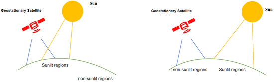
Figure 1.
Illustration of sunlit and non-sunlit regions of the Earth’s surface at different times. For reliable radar synthesis, a model must accurately differentiate between valid and noisy visible-light data.
Therefore, a static temporal boundary is insufficient to delineate valid from noisy visible-light inputs. A spatially adaptive approach is necessary to accommodate regional and seasonal variability in solar exposure, ensuring robust radar synthesis. In our framework, the illumination-aware classifier directly learns whether a given pixel is sunlit or not, providing a more physically grounded separation. This design removes noisy albedo textures during nighttime while retaining infrared-based thermodynamic signals. Compared with coarse time-window partitioning in prior studies, our adaptive method avoids spurious visible-light artifacts and ensures more stable radar synthesis across different times and regions.
2.2. Data and Preprocessing
2.2.1. Himawari-8 Imagery
This study utilized multispectral satellite observation data collected by the Himawari-8 satellite as a foundation for the development and assessment of the proposed deep-learning model. Himawari-8 is a next-generation geostationary meteorological satellite that has been operated continuously by the Japan Meteorological Agency since 7 October 2014 [21]. It is equipped with the Advanced Himawari Imager, which provides high-resolution multispectral remote sensing data covering most of the Asia–Pacific region and its surrounding areas. The observational range of the satellite (60°N–60°S, 85°–165°E) enables real-time monitoring of meteorological changes over a vast area [22]. This extensive coverage plays a vital role in early warnings of extreme weather events such as typhoons and heavy rainfall. The satellite conducts full-disk scans at 10-min intervals, offering valuable data resources for weather forecasting and environmental monitoring [23,24].
Himawari-8 captures multispectral data across 16 spectral bands, spanning visible, infrared, and near-infrared wavelengths. The visible bands provide high-resolution daytime imagery of the Earth’s surface and cloud layers, facilitating the observation of weather phenomena such as storms, cloud structures, fog, and smoke. These bands are particularly useful for daytime precipitation monitoring and storm tracking. However, visible-light data cannot adequately capture nighttime imagery and are susceptible to interference due to cloud thickness, aerosols, and atmospheric pollutants, often resulting in image blurring or increased noise levels. Figure 2 illustrates the impact of lighting conditions on visible satellite imagery.
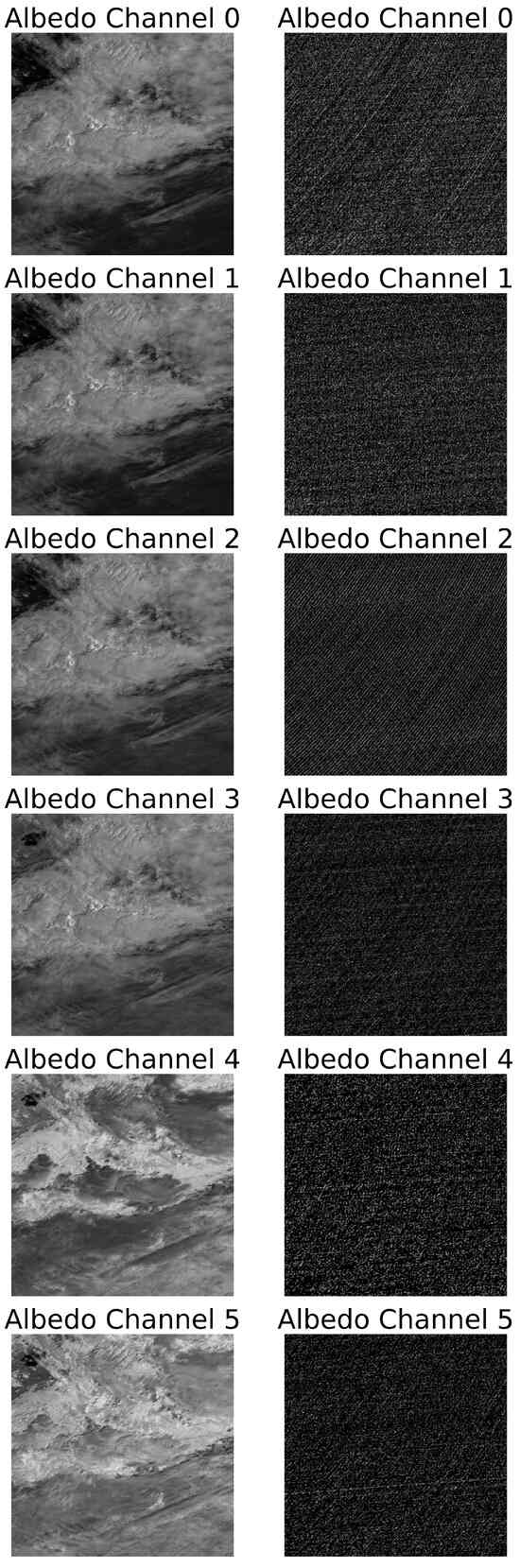
Figure 2.
Grayscale albedo images from 6 visible channels (0–5) of the Himawari-8 satellite under different illumination conditions. The left column corresponds to daytime observations at 09:00 on 21 June 2019, while the right column corresponds to nighttime observations at 23:00 on 24 June 2019. Both sets cover the same spatial region (25°–30.12°N, 100°–105.12°E). Compared with the daytime images, the nighttime images show significantly reduced albedo and increased noise, particularly in the lower channels, illustrating the impact of limited solar illumination on visible-band satellite observations.
In contrast, infrared spectral bands facilitate continuous all-weather monitoring, enabling consistent image acquisition regardless of diurnal variation. Infrared observations provide critical insights for detecting and characterizing extreme weather phenomena such as torrential rainfall and tropical cyclones through the analysis of cloud-top brightness temperature, land-surface thermal characteristics, and atmospheric water vapor distribution. Nevertheless, the lower spatial resolution of infrared data compared to visible bands compromises the delineation of fine-scale cloud structures, particularly in areas characterized by sparse cloud coverage or persistent fog conditions [25,26].
To support the synthesis of CREF from satellite data, we carefully selected 12 representative spectral bands from the Himawari-8 satellite, including visible bands (1–6) and infrared bands (8–10, 12, 14, and 15). The visible bands capture cloud optical properties such as texture, structure, and reflectance, which are valuable for analyzing cloud morphology and convective development under sufficient illumination. In contrast, the infrared bands provide critical information for continuous daytime and nighttime monitoring, including cloud-top brightness temperatures, water vapor distribution, and convective intensity. Band 10 (10.4 µm) is commonly used for monitoring cloud-top temperatures, where lower values often indicate stronger convection and heavier rainfall, whereas band 9 (6.2 µm) is sensitive to upper-tropospheric water vapor and is used for early warnings of tropical cyclones and heavy precipitation. This combination of channels offers a well-balanced synergy of spatial resolution, temporal frequency, and spectral diversity, supporting robust, adaptive CREF syntheses across diverse atmospheric conditions [21,27,28]. The Himawari-8 satellite data are available at: https://www.himawari.cloud/.
2.2.2. CREF
CREF is a core variable in radar meteorology that represents the maximum reflectivity within a vertical column by synthesizing reflectivity data from multiple elevation scans. It is used to create two-dimensional (2D) projections of storms’ structure and convective intensity for the analysis of tropospheric meteorological phenomena [29,30].
CREF provides a quantitative measure of echo intensity, which is closely related to the precipitation rate, condensation dynamics, and hydrometeor spatial distribution [9,31]. The CREF data employed in this study were derived from high-quality radar products that include base reflectivity factor information, and were used as supervisory signals in the model to evaluate the accuracy of CREF reconstruction.
The dataset was sourced from the operational radar network of the China Meteorological Administration, which integrates S-band and C-band radars. This system provides extensive spatial coverage across eastern and northeastern China, supporting meteorological monitoring, convective system tracking, and early warning of severe weather events [18,32].
The CREF data used in this study can be accessed from: https://www.cma.gov.cn/2011xwzx/ywfw/202307/t202307065631431.html.
2.2.3. Data Processing
Spatially, we implemented a rigorous coordinate-matching procedure based on identical geodetic latitude and longitude values. Temporally, we enforced a strict synchronization threshold of ±3 min to minimize temporal discrepancies.
Although both Himawari-8 and CREF products are provided at 10-min temporal resolution, we resampled both datasets to 60-min resolution before pairing (Figure 3). This downsampling approach reduced the strong temporal autocorrelation inherent in high-frequency geostationary satellite observations, avoiding redundant sampling of the same convective system within short time spans, and reducing the computational and storage requirements for long-term data processing. For temporal alignment, we applied a nearest-neighbor matching algorithm that selected the most temporally proximate CREF observation for each Himawari-8 acquisition within a ±3-min window, thereby ensuring strict one-to-one satellite–radar pairing. This procedure effectively suppressed temporal mismatches, eliminated ambiguous multiple matches, and improved the overall reliability and consistency of the integrated dataset [33].
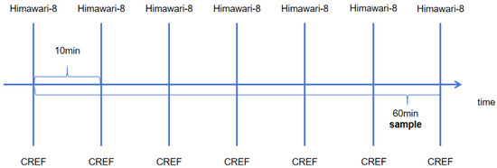
Figure 3.
Schematic illustration of the temporal downsampling and pairing strategy used in this study. Both Himawari-8 and composite reflectivity (CREF) data were originally provided at a 10-min temporal resolution (vertical bars). For dataset integration, both datasets were downsampled to 60-min resolution before pairing.
To address the spatial resolution discrepancy between the two datasets, we implemented bilinear interpolation to downscale the radar data systematically from their native 1-km resolution to 2-km resolution [34]. This spatial normalization process ensured dimensional consistency between the satellite and radar datasets, facilitating more robust data integration. To further enhance the geographical alignment between model input features and corresponding ground truth, we performed standardized cropping of the original large-scale radar and satellite data into fixed spatial domains (512 km × 512 km). This spatial standardization procedure ensured both dimensional uniformity and experimental reproducibility across all data samples.
To enhance model convergence efficiency and training stability, we implemented max–min normalization during data preprocessing. Considering that CREF radar echo measurements typically range between 0 and 80 dBZ, we applied data clipping by thresholding values below 0 to 0 and those above 80 to 80. Following this preprocessing step, we normalized the data to a [0, 1] interval through linear transformation, ensuring optimal pixel value scaling for model optimization while promoting stable and efficient convergence [35].
Furthermore, to ensure consistent numerical precision and maintain cross-modal data integrity, we standardized all input modalities, including infrared spectral data, visible-light imagery, and CREF radar measurements, to a unified 32-bit floating-point format (float32). This standardization process facilitated seamless data integration while preserving the computational accuracy required for precise radar synthesis.
Finally, to facilitate model training, validation, and cross-year evaluation, we partitioned the processed data into training, validation, and testing sets based on temporal segmentation. Data from 2018 and 2019 were used for training, those from June 2020 were used for validation, and those from July to August 2020 were reserved for testing. This partitioning strategy ensured objective model evaluation and allowed us to assess the model’s generalization ability across different years.
Following preprocessing, the data were unified in terms of both spatiotemporal resolution and numerical range, providing high-quality input for the subsequent dual-path radar synthesis network.
2.3. Model
Figure 4 illustrates the overall dual-stage architecture proposed in this study for synthesizing CREF data from Himawari-8 multispectral satellite data. The framework consists of two main stages: light/dark classification in stage I and radar synthesis in stage II.
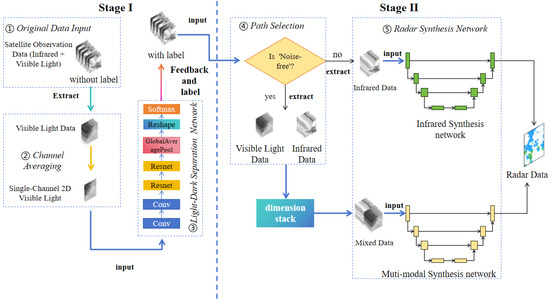
Figure 4.
Overview of the proposed dual-stage synthesis framework. Stage 1 (left) represents the light/dark classification phase, in which visible-band data are averaged spectrally and then classified as noise-free or noisy samples by the light/dark separation network. Stage 2 (right) represents the dual-path radar synthesis phase, in which noise-free data are processed by the multimodal synthesis network using both visible and infrared inputs, whereas noisy data are handled by an infrared-only synthesis network. This architecture enables adaptive, robust radar CREF synthesis under varying illumination conditions.
In stage I, well-illuminated daytime samples are differentiated from nighttime samples affected by visible-light noise, ensuring reliable input for the subsequent radar synthesis process. The key steps are as follows.
- Single-Channel 2D Feature Map Extraction. Visible-light channels are extracted and averaged across the six channels to form a single-channel 2D grayscale image that captures the overall brightness distribution while reducing input dimensionality.
- Light/Dark Separation Network. The single-channel 2D grayscale image is passed through a lightweight convolutional classifier composed of two convolution layers, residual blocks, global-average pooling, and a SoftMax layer to determine whether the input sample is noise-free (daytime) or noisy (nighttime).
- Feedback and Labeling. The classification result is used as a pseudo-label and fed back to guide automatic path selection in stage II.
In stage II, a dual-path U-Net architecture dynamically selects the appropriate processing path based on the classification output from stage I. The key steps are as follows.
- Automatic Path Selection. If the sample is classified as noise-free, both visible and infrared data are stacked and sent into the multimodal synthesis path. If the sample is classified as noisy, only infrared data are used and sent to the infrared-only synthesis path.
- Radar Synthesis Network. Both synthesis paths share the same U-Net structure for end-to-end CREF prediction. The paths differ only in terms of the numbers and types of input channels. The final output is a single-channel CREF map that maintains high synthesis quality under varying illumination conditions.
This illumination-adaptive framework significantly enhances the robustness and generalizability of radar synthesis performance across daytime and nighttime scenarios.
2.3.1. Stage I: Light/Dark Separation
In this section, we provide a detailed description of the first phase of the proposed dual-stage synthesis framework (Figure 4, stage I). The primary objective of this phase is to classify satellite data and remove visible-light noise, producing high-quality input for subsequent radar data synthesis. This synthesis phase consists of single-channel 2D visualization processing of the data, classification of the visualized data by a neural network, and feedback of the classification results to annotate the original data.
- Single-Channel 2D Feature Map Extraction.
Our satellite dataset consisted of both visible and infrared channels. Because this study focused on separating illuminated and non-illuminated scenes (i.e., light/dark separation), we primarily utilized visible-light data, which are sensitive to solar radiation. The Himawari-8 satellite provides six visible channels (bands 1–6), each capturing reflected solar radiation in different spectral ranges. Together, these bands contain rich information about surface albedo, cloud reflectance, and atmospheric scattering under varying illumination conditions. Using only a single channel can result in unreliable assessments due to local noise or occlusion. To address this issue, we adopted a spectral band-averaging strategy to generate a robust 2D grayscale representation by integrating all six visible channels. The averaged pixel value for each location is computed as follows:
where C is the number of visible channels (6 in this study), and represents the pixel value at location in the c-th channel.
This operation reduces spectral variance while enhancing the consistency of brightness information across channels. The resulting single-channel 2D grayscale image is a more reliable proxy for detecting whether a scene is illuminated. It remains visually robust even in the presence of channel-specific noise, and therefore represents a foundational feature for downstream tasks such as noise-aware data selection and light/dark classification.
- Light/Dark Separation Network Structure.
Next, the obtained single-channel 2D visible-light data are entered into our separation network for processing. The entire network structure is a convolutional residual network. The single-channel 2D feature map X passes through a feature extraction layer composed of two convolutional layers to obtain deeper features (). This process is described as follows:
Afterward, the extracted is input into the residual network layers, undergoes two residual block processes, as follows:
The residual network structure is shown in Figure 5.
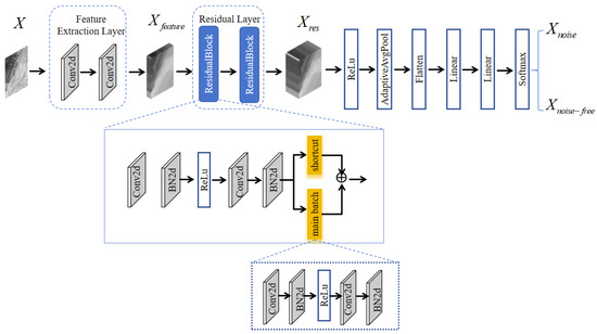
Figure 5.
Residual network structure for light/dark separation.
This integration method effectively preserves input feature information, allowing the network to extract multi-level image features more stably during training. It significantly reduces the common gradient-vanishing problem in deep networks, improving classification accuracy and generalization under varying illumination conditions. Finally, is passed through a global-average pooling layer and multiple classification layers to obtain the final classification targets: and .
- Feedback and Labeling of Noisy Data.
The classification results are fed back into the original satellite observation dataset from the single-channel 2D feature map. At this point, each satellite observation dataset is labeled with the illumination condition, as (no light) and (with light). Visible-light channels with no-light data are automatically masked during radar synthesis. The classification criteria are described in detail in Section 2.4.
2.3.2. Stage II: Radar Synthesis Network Structure
In the second phase of the proposed dual-stage synthesis framework (Figure 4, stage II), labeled data based on the light/dark classification results are automatically identified, and the clean samples are fed into the corresponding radar synthesis network to generate CREF data. The structure of the synthesis network is shown in Figure 6.
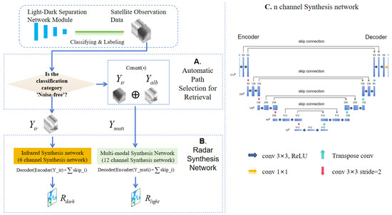
Figure 6.
Radar synthesis network structure. (A) Path selection following automatic identification of labeled data. (B) CREF synthesis. (C) Synthesis architecture used for CREF synthesis. The synthesis networks shown in (B) were derived from the architecture shown in (C), with different input channels.
The radar synthesis network used in this study was designed based on the U-Net architecture, which was adopted for its outstanding ability to preserve spatial resolution and capture multi-scale contextual features, which are crucial attributes for high-precision radar image generation. The symmetric encoder–decoder structure of U-Net, combined with skip connections, effectively integrates global and local features, making it particularly suitable for mapping satellite data to CREF, as the target features (e.g., cloud morphology and convective cores) require both high-level semantic information and fine-grained spatial localization. U-Net has demonstrated strong robustness to noise and missing data in remote sensing and meteorological image reconstruction tasks. Although the visible-light channel data used in this study were initially denoised, the U-Net feature fusion mechanism can mitigate any remaining minor inconsistencies via skip connections, improving synthesis accuracy.
- Automatic Path Selection Mechanism.
Based on the light/dark classification results, data are divided into noisy (nighttime or insufficient illumination) and noise-free (daytime or sufficient illumination) samples, and the corresponding synthesis path is automatically selected (Figure 6A). For noisy data, only the infrared channel () is used as input for radar synthesis, whereas for noise-free data, and the visible-light channel ) are concatenated along the channel dimension to form a 12-channel multimodal input, as follows:
- Dual-Path Radar Synthesis Network Structure.
After automatic path selection, the data are fed into different synthesis networks for dual-path CREF synthesis (Figure 6B). The infrared synthesis network processes infrared data (), and the multimodal synthesis network processes multimodal data (). Although these input data types differ, both paths employ the n-channel U-Net synthesis network shown in Figure 6C, differing only in the number of input channels.
The U-Net network consists of an encoder and a decoder. A sequence of feature-compression modules forms the encoder, which consists of a series of convolution layers and stride-2 downsampling layers (Figure 6C, left), progressively reducing the spatial resolution. The decoder consists of a sequence of feature-restoration modules (Figure 6C, right) that progressively restore spatial resolution using transposed convolutions and fuse features from the corresponding encoder layers via skip connections to retain spatial details.
For the encoder, we assign the input as X and compute the feature map output of the ith encoder layer , as follows:
where X can be either or , depending on the selected network.
In the decoding stage, skip connections sum the upsampled decoder features with the corresponding encoder features, as follows:
Finally, radar synthesis results are obtained for different illumination conditions (nighttime/noisy conditions and daytime/noise-free conditions), as follows:
- Nighttime or noisy conditions:
- Daytime or noise-free conditions:
where denotes the skip connection features at resolution level i, which enhance the spatial reconstruction capability of the decoder. This framework dynamically adjusts the number of input channels (6 or 12) according to illumination conditions, maintaining network structural consistency while improving CREF synthesis performance under varying lighting conditions.
Physically, this dual-path design reflects the complementary roles of infrared and visible observations: infrared brightness temperature captures cloud-top thermodynamics and is reliable under all illumination conditions, whereas visible-light imagery provides fine-scale optical texture that is useful only under conditions of sufficient sunlight. By assigning noisy nighttime inputs exclusively to the infrared path and daytime inputs to the multimodal path, the model avoids forcing a single network to compromise between incompatible feature statistics.
2.4. Model Training
We carefully designed the experimental framework and parameter configurations to ensure the fairness and objectivity of our experimental evaluation. Key aspects of our methodology are described below.
2.4.1. Design of the Loss Function
Because our training process involves two stages, the light/dark separation network and the radar synthesis network, we designed different loss functions to meet the objectives of each network. For the light/dark separation task, we employed the standard cross-entropy loss function [36], defined as follows:
where is the ground-truth label, is the predicted probability for the corresponding class, and N is the total number of samples.
For the radar synthesis task based on satellite observations, we employ a weighted mean absolute error (MAE) loss function to address the imbalance between weak and strong precipitation events. Unlike the conventional MAE, which treats all pixels equally, our loss introduces pixel-wise, reflectivity-dependent weights to emphasize meteorologically significant regions. Specifically, higher weights are assigned to pixels with strong radar reflectivity (e.g., convective cores), while weaker echoes receive smaller weights. This design enables the model to focus more on critical structures rather than being dominated by the large number of weak or no-precipitation pixels.
Formally, the weighted MAE is defined as:
where N is the number of pixels, is the ground-truth reflectivity, is the prediction, and is the pixel-wise weight.
For practical training stability, we discretized the reflectivity into 5 dBZ bins and approximated the weights from Equation (11) into integer values, resulting in the following scheme used in our experiments:
Inspired by the pixel-wise weighting strategies in TrajGRU [37] and Pixel-CRN [38], we adopt an empirical weighting scheme to enhance learning in meteorologically critical regions. By emphasizing high-reflectivity areas while still considering weak echoes, this strategy enables the model to more accurately reconstruct convective structures and intense precipitation, thereby improving synthesis accuracy in severe weather scenarios.
2.4.2. Training of the Light-Dark Separation Module
To ensure that the light/dark separation module could automatically classify and identify visible-light data, we pretrained it on a dataset selected based on the following criteria: single-channel 2D feature maps obtained by spectral band-averaging (see Section 1) were used as the base data, and an expert-driven classification approach was used to assign labels [39]. Based on classification standards from current literature, the expert classification method divided samples into normal-illumination (noise-free) and low-illumination (noisy) images (Figure 7). The former category included standard daytime images with well-defined cloud structures and minimal noise contamination, and nighttime images without visible noise artifacts; classification was based on the absence of pixel intensity variation or structural artifacts. Low-illumination images included those showing prominent noise artifacts, such as irregular bright spots or streaks. These images contained various sources of noise interference, such as thermal, photon, and readout noise [16,40].
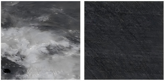
Figure 7.
Two-dimensional single-channel visualization results for normal-illumination (left) and low-illumination (right) images based on satellite data.
During the training phase, we used the cross-entropy loss function defined in Section 2.4.1 and optimized the model parameters using the Adam optimizer with a learning rate of [41].
The trained light/dark noise classification network achieved perfect classification accuracy (100%) in distinguishing noise-degraded nighttime images from noise-free images, demonstrating its effectiveness as a preprocessing component for radar synthesis [42].
2.4.3. Training for Radar Synthesis Stage
After training the light/dark separation module, we froze its parameters and linked them to our dual-path radar synthesis network to reconstruct radar data. We used the weighted loss function described in Section 2.4.2 for loss computation and employed the Adam optimizer with an initial learning rate of , combined with cosine annealing for dynamic learning rate adjustment. This method allowed more efficient convergence and enhanced global optimization performance.
Our training and testing stages were designed differently (Figure 8). In the training phase of our radar synthesis framework, regardless of the assigned classification label, the infrared synthesis network processed six-channel infrared spectral data, ensuring consistent feature extraction under all conditions. This approach significantly enhanced the model’s generalization ability and operational robustness by systematically exposing it to various illumination scenarios and environmental conditions [43]. For standard daytime images, the 12-channel multimodal synthesis network processed both visible-light data and 6-channel infrared data, enriching feature space representation and facilitating comprehensive radar image reconstruction with enhanced spatial and spectral fidelity.
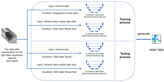
Figure 8.
Diagram of the training and testing processes.
During the inference and testing phases, the infrared synthesis network was used solely to synthesize data labeled as noise, whereas the multimodal synthesis network was used exclusively to synthesize data labeled as noise-free.
3. Result
3.1. Evaluation Metrics
To assess the performance of radar synthesis both comprehensively and objectively, we adopted a set of metrics that are well suited to evaluating radar data reconstruction characteristics. Traditional regression-based indicators such as mean square error (MSE) and mean absolute error (MAE) primarily assess pixel-level differences, which can fail to reflect the effectiveness of a model in capturing meteorologically significant structures, particularly in scenarios that involve strong convective echoes or heavy precipitation.
Therefore, we applied detection-oriented evaluation metrics that are widely used in meteorological forecast verification: the false alarm ratio (FAR), probability of detection (POD), critical success index (CSI), and frequency bias (Bias). These metrics are derived from the four fundamental components of the confusion matrix: true positives (TP), false positives (FP), false negatives (FN), and true negatives (TN).
POD evaluates a model’s ability to detect meaningful radar signals by quantifying the proportion of correctly predicted positive cases among all actual positives. A higher POD indicates stronger sensitivity to true precipitation regions. In contrast, the FAR is calculated as the frequency at which non-relevant regions are incorrectly classified as significant radar signals. A lower FAR implies better precision and fewer false alarms. The CSI jointly considers hits, misses, and false alarms, thus providing a comprehensive, balanced assessment of overall radar synthesis performance.
In addition, the frequency bias (FBIAS) metric was included to evaluate whether the model systematically overestimates or underestimates the occurrence of precipitation events [44]. An FBIAS value greater than 1 indicates overestimation (too many predicted events), while a value less than 1 indicates underestimation (too few predicted events). This complementary metric provides further insight into the model’s prediction tendencies and enhances the interpretability of the evaluation results.
To further ensure fairness and robustness, we report a weighted average CSI score that accounts for results from both the infrared-only U-Net and the mixed-data U-Net models. In calculating the overall score, the number of test samples in each configuration was used as a weighting factor, allowing a unified comparison across data types.
3.2. Experimental Results
Under high-echo convective conditions (≥35 dBZ), the experimental results demonstrate the reliability and robustness of the 6-channel and 12-channel models in detecting convective events within their respective operating environments. The infrared-based model had a low FAR (0.4360) under nighttime noise conditions, showing superior noise suppression capability that significantly enhanced model detection accuracy. The mixed-data model achieved high POD (0.5171) and CSI (0.3306) values under noise-free daytime conditions, demonstrating its exceptional performance in convective event detection through effective multi-channel feature fusion.
Our model outperformed other approaches in terms of the CSI and POD (Table 1, Table 2 and Table 3), indicating its higher success rate in accurately identifying severe weather events. However, the relatively high FAR implies that there is room for further optimization in reducing false positives.

Table 1.
Critical success index (CSI) evaluation results at different radar composite reflectivity (CREF) thresholds (dBZ). CSI_6 refers to results from the 6-channel infrared-only U-Net model; CSI_12 refers to results from the 12-channel multimodal (infrared + visible) U-Net model. Avg_CSI is a weighted average calculated based on the number of test samples for each configuration.
Table 2.
Probability of detection (POD) evaluation results at different CREF thresholds (dBZ). POD_6 refers to results from the 6-channel infrared-only U-Net model; POD_12 refers to results from the 12-channel multimodal (infrared + visible) U-Net model. Avg_POD is a weighted average calculated based on the number of test samples for each configuration.
Table 3.
False alarm rate (FAR) evaluation results at different CREF thresholds (dBZ). FAR_6 refers to results from the 6-channel infrared-only U-Net model; FAR_12 refers to results from the 12-channel multimodal (infrared + visible) U-Net model. Avg_FAR is a weighted average calculated based on the number of test samples for each configuration.
In addition, we calculated the frequency bias (FBias) values across different thresholds to further assess whether the models tend to overestimate or underestimate precipitation events. As shown in Table 4, the FBias values are close to 1 at 20 dBZ, suggesting nearly unbiased performance at moderate precipitation levels. At lower thresholds (10 dBZ), both models slightly over-predict precipitation events, while at higher thresholds (30–35 dBZ), both models exhibit mild underestimation.
Table 4.
Frequency bias (FBias) evaluation results at different CREF thresholds (dBZ). FBias_6 refers to results from the 6-channel infrared-only U-Net model; FBias_12 refers to results from the 12-channel multimodal (infrared + visible) U-Net model. Avg_FBias is a weighted average calculated based on the number of test samples for each configuration.
These findings objectively validate the effectiveness of both detection strategies under nighttime noisy and daytime noise-free conditions, and confirm the feasibility of adjusting detection strategies based on data characteristics. This approach will be useful in convective event detection across different scenarios and is anticipated to contribute to the development of more robust early warning systems.
To further verify the effectiveness of the proposed framework, we conducted comparison experiments with GAN and Swin-UNet models, using the same loss function (Weighted-MAE) to ensure fairness. As shown in Figure 9, despite having significantly larger parameter sizes, both models failed to surpass our approach. Specifically, our model more effectively reconstructs the spatial structures of precipitation: it preserves the integrity of convective cloud clusters better than Swin-UNet, avoiding fragmented boundaries and sparse echoes, while also suppressing the spurious artifacts often produced by GAN. In strong echo regions (red and dark red), it accurately maintains reflectivity intensity and distribution, whereas in weak echo regions (blue and green), it produces continuous and physically coherent patterns without artificial scattered patches. Furthermore, the model captures finer structural details along small-scale cloud clusters and echo boundaries, yielding closer agreement with radar observations. These results highlight the efficiency, robustness, and reliability of our framework in reproducing precipitation echoes, which is particularly valuable for short-term forecasting and early warning of severe convective weather.
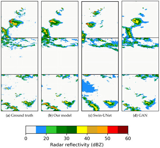
Figure 9.
Comparison of CREF synthesis: (a) Ground truth, (b) Our model, (c) Swin-UNet, and (d) GAN.
3.3. Ablation Experiments
To evaluate the effectiveness of the proposed light/dark separation strategy in CREF synthesis tasks, we conducted a set of ablation experiments. To determine whether prior differentiation of noisy and noise-free data would enhance overall model performance, we compared the performance of our dual-path method with that of the conventional U-Net, which performs radar synthesis directly without noise-aware separation.
For fair comparison, both the baseline U-Net and our proposed dual-path model were trained using the Weighted MAE loss function, consistent with the setup described in Section 2.4. This ensured that the observed performance differences were solely due to the use of the light/dark separation strategy rather than variations in training objectives.
We evaluated both models according to CSI, POD, FAR, and Bias across different CREF thresholds (10, 20, 30, 35, and 40 dBZ). The proposed model significantly outperformed U-Net in terms of CSI and POD at most thresholds (Table 5). This advantage was particularly notable in high-reflectivity scenarios (e.g., ≥30 dBZ). For example, at the 35-dBZ threshold, our method achieved a CSI of 0.6142 and POD of 0.7859, compared with 0.5191 and 0.7111 for U-Net, respectively. These results clearly demonstrate that our strategy yields more robust, accurate detection results for heavy precipitation areas.
Table 5.
Comparison of performance metrics (CSI, POD, FAR, and FBias) between the proposed model and U-Net across different CREF thresholds.
Bias analysis further revealed the advantages of our method (Table 5). At low thresholds (10 and 20 dBZ), both models slightly overestimated precipitation events, with FBias values > 1. However, our model remained closer to unbiased (FBias = 1.176 at 10 dBZ and 1.024 at 20 dBZ) compared to the U-Net (1.321 and 1.152, respectively). At higher thresholds (30 and 35 dBZ), the baseline U-Net yielded stronger underestimation (FBias = 0.649 and 0.601, respectively), while our model maintained values closer to 1 (0.910 and 0.883, respectively), indicating a more balanced prediction tendency. At the extreme threshold of 40 dBZ, both models underestimated rare convective events, but our model (Bias = 0.592) clearly outperformed U-Net (Bias = 0.292), capturing nearly twice as many of the extreme cases.
As shown in Figure 10, our method produces radar reflectivity fields that are more consistent with the ground truth compared to the traditional approach. In particular, false alarms in regions with reflectivity values exceeding 35 dBZ are clearly reduced. This indicates that the illumination-aware classification and dual-path synthesis strategy effectively suppresses spurious convective echoes that often arise under low-light or transitional conditions. As a result, the generated high-reflectivity areas better align with the actual convective structures, improving the overall reliability of the synthesized radar fields.
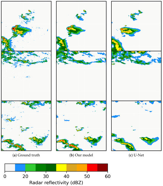
Figure 10.
Comparison of model visual outputs. (a) Ground truth image; (b) our model (c) U-Net.
In summary, our ablation experiments provided both quantitative and qualitative evidence validating the effectiveness of the proposed light/dark separation strategy. By inputting noisy data into the infrared-based synthesis network and noise-free data into the multimodal network, our model achieved better targeted learning for different input types, improving CREF synthesis accuracy and enhancing its responsiveness to severe weather conditions.
4. Case Studies Exploring Temporal and Regional Variations in Illumination
To illustrate further the limitations of time-based classification in radar synthesis, we conducted two case studies with temporal and spatial inconsistencies in early-morning conditions. These studies evaluated how variations in sunrise timing and regional daylight exposure impact synthesis performance.
4.1. Case Study I: Impact of Sunrise Time Across Seasons
We selected two representative datasets, one from July 2018 (near the summer solstice) and one from December 2018 (near the winter solstice), focusing on satellite data captured from 3:00 to 7:00. In both cases, we used 6:00 as the boundary between night and day, such that data captured before 6:00 were treated as nighttime data, and those captured from 6:00 to noon were classified as daytime data.
This case study evaluated the effectiveness of time-based data division in different seasons. In July, sunrise occurs earlier, potentially making visible-light data usable before the 6:00 threshold. Conversely, in December, a delayed sunrise may result in the inclusion of noisy visible images if classification is based purely on time.
Radar synthesis performance was assessed using the CSI values across different timestamps. CSI values around 6:00 in July increased due to the earlier sunrise (Figure 11), which enabled more effective use of visible channels. In contrast, CSI values in December decreased around 6:00 due to noise, highlighting the limitations of static time-based segmentation.
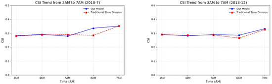
Figure 11.
Synthesis CSI trends for different timestamps. Results are shown for July 2018 (left) and December 2018 (right), demonstrating a clear impact of sunrise timing on synthesis quality.
4.2. Case Study II: Regional Variations in Illumination
To explore spatial inconsistencies caused by fixed time segmentation, we selected data from 6:00 on 25 June 2019, covering both the eastern coastal (25.51°N∼35.75°N, 99.12°E∼109.24°E) and western inland (20.39°N∼30.63°N, 94.00°E∼109.24°E) regions of China. The study area was divided into multiple 512 km2 sub-regions to evaluate synthesis consistency under uniform time-based classification. The results demonstrate significant sunrise timing variation across these regions, resulting in non-uniform illumination conditions. This discrepancy introduced visible channel noise in western regions when using a fixed classification time, thereby reducing radar synthesis accuracy.
To assess this effect quantitatively, we calculated the CSI for each sub-region at reflectivity thresholds of ≥35 dBZ (denoted as ) using the conventional U-Net synthesis model, and performed a comparative analysis. Figure 12 illustrates the trend from east to west, clearly showing performance degradation toward the west due to earlier data classification.
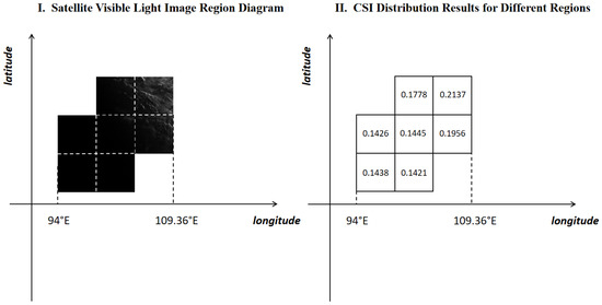
Figure 12.
Illustration of the impact of regional variation in sunrise time on radar synthesis performance. (Left) Spatial layout of the selected sub-regions. (Right) CSI values at reflectivity thresholds of ≥35 dBZ (denoted as ) for each sub-region.
4.3. Case Study III: Daytime Subset Comparison of Multimodal and Infrared-Only Models
To further evaluate the necessity of multimodal input under conditions of sufficient daylight, we selected a 6-channel infrared-only U-Net model trained with daytime infrared data as the infrared-only baseline, and compared it with our pretrained 12-channel multimodal U-Net model (infrared + visible). The synthesized test results are presented in Figure 13.
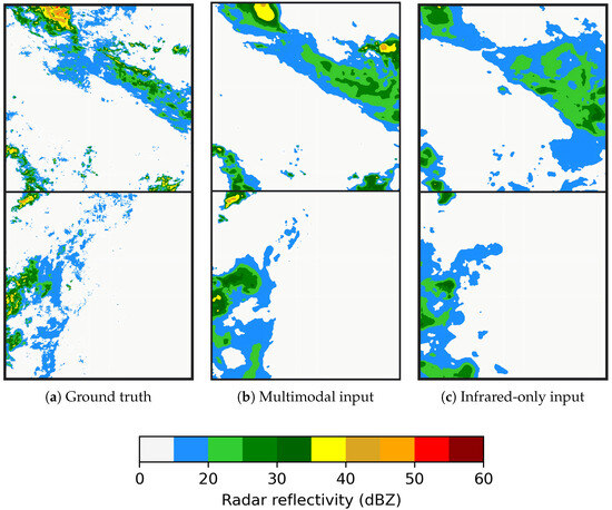
Figure 13.
Necessity of multimodal input under sufficient daylight conditions: (a) Ground truth, (b) Multimodal input, and (c) Infrared-only input.
From the comparison, it can be observed that the model trained solely on infrared observations performs effectively at low thresholds (10–30 dBZ), but shows significant deficiencies in the high-threshold region (≥35 dBZ). This demonstrates that infrared information is sufficient for synthesizing low-reflectivity echoes, whereas the inclusion of visible channels provides clear benefits in identifying strong convective structures at higher reflectivity levels.
These findings highlight the necessity of multimodal input for the retrieval of strong convection (composite reflectivity ≥35 dBZ).
5. Discussion and Conclusions
This study proposes an illumination-based classification and dual-path processing framework for synthesizing radar reflectivity from geostationary satellite observations. Compared with the traditional U-Net model, the proposed approach demonstrates significant improvements in the reconstruction of radar reflectivity within convective regions, achieving higher Critical Success Index (CSI) and Probability of Detection (POD) values while substantially reducing the False Alarm Rate (FAR). These results indicate that the illumination-aware and dual-path fusion strategy effectively enhances the stability and accuracy of satellite-based radar synthesis.
The improved model performance can be attributed primarily to two mechanisms:
- (1)
- The illumination classification module enables the distinction between daytime and nighttime imagery, thereby mitigating noise contamination caused by visible-band degradation under low-light conditions. The results clearly show that nighttime noise significantly affects the quality of radar synthesis. Properly separating noisy nighttime visible-light data improves the accuracy of radar reconstruction, while retaining as much usable visible-light information as possible also helps enhance the synthesis quality. This demonstrates the feasibility and effectiveness of our illumination-based classification mechanism.
- (2)
- The multimodal input simultaneously exploits features from both infrared (IR) and visible (VIS) channels, allowing the model to capture the thermodynamic and optical structures of convective systems, which further improves the quality of synthesized radar reflectivity. The results show that radar synthesized solely from infrared channels still exhibits a certain degree of underestimation, particularly within intense convective regions. When visible-light information is incorporated, the cloud structures become more clearly defined, leading to more accurate radar synthesis in strong convective cores. According to related studies, this underestimation primarily arises from the limited penetration capability of infrared radiation, which prevents the retrieval of realistic reflectivity features from within deep convective clouds [45]. As a result, the model relies more heavily on cloud-top brightness temperature gradients while underrepresenting internal convective structures [46]. This further confirms the importance and necessity of using multimodal data in radar synthesis.
Of course, this study also reveals certain limitations. During extreme convective weather events, the model performance tends to degrade, mainly due to the limited number of such samples in the training dataset. Severe convection is characterized by its sporadic and localized nature, resulting in a serious data imbalance that constrains the generalization capability of deep-learning models. To mitigate this issue, future research should employ data augmentation strategies that account for meteorological regularities in both spatial (latitude–longitude) and temporal domains, in order to enhance the model’s ability to learn from rare but crucial convective systems [47].
In summary, this study confirms the effectiveness of the proposed illumination-aware classification and dual-path fusion framework in improving the accuracy and stability of satellite-based radar reflectivity synthesis. The proposed approach not only achieves high-quality radar reconstruction over eastern China but also demonstrates potential applicability to radar-sparse regions, such as oceans and complex terrains. Future work will focus on expanding the spatial–temporal coverage of the training dataset, optimizing the multimodal data fusion structure, and improving prediction performance for strong convective regions.
Author Contributions
Conceptualization, X.S., C.L. and H.L.; Methodology, W.Z., H.M., J.D. and R.P.; Software, H.M. and R.P.; Validation, H.M.; Formal analysis, W.Z., H.M., Y.G., J.D., R.P. and X.S.; Investigation, W.Z., Y.G., J.D. and H.L.; Resources, W.Z., R.P., C.L. and H.L.; Data curation, H.M.; Writing—original draft, W.Z. and H.M.; Writing—review & editing, W.Z., H.M., Y.G. and X.S.; Visualization, C.L.; Supervision, J.D.; Project administration, W.Z., R.P. and X.S.; Funding acquisition, W.Z. All authors have read and agreed to the published version of the manuscript.
Funding
This work was supported by the National Natural Science Foundation of China under Grant 42276202.
Data Availability Statement
The original contributions presented in this study are included in the article. Further inquiries can be directed to the corresponding author.
Conflicts of Interest
Authors Cong Liu and Hongmei Liu were employed by the company China Mobile Group Shandong Co., Ltd. The remaining authors declare that the research was conducted in the absence of any commercial or financial relationships that could be construed as a potential conflict of interest.
References
- Racah, E.; Beckham, C.; Maharaj, T.; Ebrahimi Kahou, S.; Prabhat, M.; Pal, C. Extremeweather: A large-scale climate dataset for semi-supervised detection, localization, and understanding of extreme weather events. In Proceedings of the 31st International Conference on Neural Information Processing Systems, Long Beach, CA, USA, 4–9 December 2017. [Google Scholar]
- Taszarek, M.; Brooks, H.E.; Czernecki, B. Sounding-derived parameters associated with convective hazards in Europe. Mon. Weather. Rev. 2017, 145, 1511–1528. [Google Scholar] [CrossRef]
- Kober, K.; Tafferner, A. Tracking and nowcasting of convective cells using remote sensing data from radar and satellite. Meteorol. Z. 2009, 1, 75–84. [Google Scholar] [CrossRef] [PubMed]
- Burcea, S.; Cică, R.; Bojariu, R. Radar-derived convective storms’ climatology for the Prut River basin: 2003–2017. Nat. Hazards Earth Syst. Sci. 2019, 19, 1305–1318. [Google Scholar] [CrossRef]
- Huang, Y.; Wang, J.; Cai, L.; Fan, Y.; Wang, H.; Zhang, T. Relationship between radar reflectivity thresholds and very low frequency/low frequency total lightning for thunderstorm identification. High Voltage 2024, 9, 1068–1080. [Google Scholar] [CrossRef]
- Yang, L.; Zhao, Q.; Xue, Y.; Sun, F.; Li, J.; Zhen, X.; Lu, T. Radar composite reflectivity reconstruction based on FY-4A using deep learning. Sensors 2022, 23, 81. [Google Scholar] [CrossRef]
- Liu, Z.; Min, M.; Li, J.; Sun, F.; Di, D.; Ai, Y.; Li, Z.; Qin, D.; Li, G.; Lin, Y.; et al. Local severe storm tracking and warning in pre-convection stage from the new generation geostationary weather satellite measurements. Remote Sens. 2019, 11, 383. [Google Scholar] [CrossRef]
- Sun, L.; Zhuge, X.; Zhu, S. Geostationary Satellite-Based Overshooting Top Detections and Their Relationship to Severe Weather over Eastern China. Remote Sens. 2024, 16, 2015. [Google Scholar] [CrossRef]
- Sun, F.; Li, B.; Min, M.; Qin, D. Deep learning-based radar composite reflectivity factor estimations from Fengyun-4A geostationary satellite observations. Remote Sens. 2021, 13, 2229. [Google Scholar] [CrossRef]
- Enos, G.R.; Reagor, M.J.; Henderson, M.P.; Young, C.; Horton, K.; Birch, M.; Rigetti, C. Synthetic weather radar using hybrid quantum-classical machine learning. arXiv 2021, arXiv:2111.15605. [Google Scholar] [CrossRef]
- Chen, H.; Chandrasekar, V.; Cifelli, R.; Xie, P. A machine learning system for precipitation estimation using satellite and ground radar network observations. IEEE Trans. Geosci. Remote Sens. 2019, 58, 982–994. [Google Scholar] [CrossRef]
- Hsu, K.L.; Gao, X.; Sorooshian, S.; Gupta, H.V. Precipitation Estimation from Remotely Sensed Information Using Artificial Neural Networks. J. Appl. Meteorol. 1997, 36, 1176–1190. [Google Scholar] [CrossRef]
- Sadeghi, M.; Asanjan, A.A.; Faridzad, M.; Nguyen, P.; Hsu, K.; Sorooshian, S.; Braithwaite, D. PERSIANN-CNN: Precipitation estimation from remotely sensed information using artificial neural networks–convolutional neural networks. J. Hydrometeorol. 2019, 20, 2273–2289. [Google Scholar] [CrossRef]
- Wang, C.; Xu, J.; Tang, G.; Yang, Y.; Hong, Y. Infrared precipitation estimation using convolutional neural network. IEEE Trans. Geosci. Remote Sens. 2020, 58, 8612–8625. [Google Scholar] [CrossRef]
- Kim, Y.; Hong, S. Hypothetical ground radar-like rain rate generation of geostationary weather satellite using data-to-data translation. IEEE Trans. Geosci. Remote Sens. 2023, 61, 1–14. [Google Scholar] [CrossRef]
- Yao, J.; Du, P.; Zhao, Y.; Wang, Y. Simulating Nighttime Visible Satellite Imagery of Tropical Cyclones Using Conditional Generative Adversarial Networks. arXiv 2024, arXiv:2401.11679. [Google Scholar] [CrossRef]
- Mills, S.; Weiss, S.; Liang, C. VIIRS day/night band (DNB) stray light characterization and correction. In Proceedings of the Earth Observing Systems XVIII, San Diego, CA, USA, 25–29 August 2013; Volume 8866, pp. 549–566. [Google Scholar]
- Min, M.; Zheng, J.; Zhang, P.; Hu, X.; Chen, L.; Li, X.; Huang, Y.; Zhu, L. A low-light radiative transfer model for satellite observations of moonlight and earth surface light at night. J. Quant. Spectrosc. Radiat. Transf. 2020, 247, 106954. [Google Scholar] [CrossRef]
- Kim, J.H.; Ryu, S.; Jeong, J.; So, D.; Ban, H.J.; Hong, S. Impact of satellite sounding data on virtual visible imagery generation using conditional generative adversarial network. IEEE J. Sel. Top. Appl. Earth Obs. Remote Sens. 2020, 13, 4532–4541. [Google Scholar] [CrossRef]
- Wang, Z.; Román, M.O.; Kalb, V.L.; Miller, S.D.; Zhang, J.; Shrestha, R.M. Quantifying uncertainties in nighttime light retrievals from Suomi-NPP and NOAA-20 VIIRS Day/Night Band data. Remote Sens. Environ. 2021, 263, 112557. [Google Scholar] [CrossRef]
- Bessho, K.; Date, K.; Hayashi, M.; Ikeda, A.; Imai, T.; Inoue, H.; Kumagai, Y.; Miyakawa, T.; Murata, H.; Ohno, T.; et al. An introduction to Himawari-8/9—Japan’s new-generation geostationary meteorological satellites. J. Meteorol. Soc. Jpn. Ser. II 2016, 94, 151–183. [Google Scholar] [CrossRef]
- Govekar, P.; Griffin, C.; Embury, O.; Mittaz, J.; Beggs, H.M.; Merchant, C.J. Himawari-8 Sea Surface Temperature Products from the Australian Bureau of Meteorology. Remote Sens. 2024, 16, 3381. [Google Scholar] [CrossRef]
- Sulistiyono, W.; Tuna, M.S.; Ramadhan, S.A. Pemanfaatan Data Satelit Himawari-8 Dalam Analisa Kejadian Hujan Lebat Di Jombang Tanggal 1–2 Februari 2021. Time Phys. 2024, 2, 31–40. [Google Scholar] [CrossRef]
- Zhang, C.; Zhuge, X.; Yu, F. Development of a high spatiotemporal resolution cloud-type classification approach using Himawari-8 and CloudSat. Int. J. Remote Sens. 2019, 40, 6464–6481. [Google Scholar] [CrossRef]
- Sun, H.; Wang, D.; Han, W.; Yang, Y. Quantifying the impact of aerosols on geostationary satellite infrared radiance simulations: A study with Himawari-8 AHI. Remote Sens. 2024, 16, 2226. [Google Scholar] [CrossRef]
- Do, H.N.; Ngo, T.X.; Nguyen, A.H.; Nguyen, T.T.N. Precipitation Estimation from Himawari-8 Multiple Spectral Channels Using U-Net. In Proceedings of the 2023 15th International Conference on Knowledge and Systems Engineering (KSE), Ha Noi, Vietnam, 18–20 October 2023; pp. 1–6. [Google Scholar]
- Nishiyama, G.; Suzuki, Y.; Uno, S.; Aoki, S.; Iwanaka, T.; Imamura, T.; Fujii, Y.; Müller, T. Temporal Variation of Venus Brightness Temperature Seen by the Japanese Meteorological Satellite Himawari-8/9. In Proceedings of the Europlanet Science Congress, Berlin, Germany, 8–13 September 2024. Technical Report, Copernicus Meetings. [Google Scholar]
- Broomhall, M.A.; Majewski, L.J.; Villani, V.O.; Grant, I.F.; Miller, S.D. Correcting Himawari-8 Advanced Himawari Imager Data for the Production of Vivid True-Color Imagery. J. Atmos. Ocean. Technol. 2019, 36, 427–442. [Google Scholar] [CrossRef]
- Chen, Y.; Chen, J.; Chen, D.; Xu, Z.; Sheng, J.; Chen, F. A simulated radar reflectivity calculation method in numerical weather prediction models. Weather Forecast. 2021, 36, 341–359. [Google Scholar] [CrossRef]
- Doviak, R.J.; Zrnic, D.S. Doppler Radar & Weather Observations; Academic Press: Cambridge, MA, USA, 2014. [Google Scholar]
- Rauber, R.M.; Nesbitt, S.W. Radar Meteorology: A First Course; John Wiley & Sons: Hoboken, NJ, USA, 2018. [Google Scholar]
- Wen, Y.; Zhang, J.; Wang, D.; Peng, X.; Wang, P. A Quantitative Precipitation Estimation Method Based on 3D Radar Reflectivity Inputs. Symmetry 2024, 16, 555. [Google Scholar] [CrossRef]
- Zhang, X.; Gao, F.; Wang, J.; Ye, Y. Evaluating a spatiotemporal shape-matching model for the generation of synthetic high spatiotemporal resolution time series of multiple satellite data. Int. J. Appl. Earth Obs. Geoinf. 2021, 104, 102545. [Google Scholar] [CrossRef]
- Press, W.H. Numerical Recipes 3rd Edition: The Art of Scientific Computing; Cambridge University Press: Cambridge, UK, 2007. [Google Scholar]
- Mining, W.I.D. Data mining: Concepts and techniques. Morgan Kaufinann 2006, 10, 4. [Google Scholar]
- Rumelhart, D.E.; Hinton, G.E.; Williams, R.J. Learning representations by back-propagating errors. Nature 1986, 323, 533–536. [Google Scholar] [CrossRef]
- Shi, X.; Gao, Z.; Lausen, L.; Wang, H.; Yeung, D.Y.; Wong, W.K.; Woo, W.C. Deep learning for precipitation nowcasting: A benchmark and a new model. In Proceedings of the 31st International Conference on Neural Information Processing Systems, Long Beach, CA, USA, 4–9 December 2017. [Google Scholar]
- Zhang, W.; Chen, H.; Han, L.; Zhang, R.; Ge, Y. Pixel-CRN: A new machine learning approach for convective storm nowcasting. IEEE Trans. Geosci. Remote Sens. 2023, 61, 1–12. [Google Scholar] [CrossRef]
- Jähne, B. Digital Image Processing; Springer Science & Business Media: Berlin/Heidelberg, Germany, 2005. [Google Scholar]
- Wang, W.; Zhong, X.; Su, Z.; Li, D.; Guo, Z. Signal-to-Noise Ration Evaluation of Luojia 1-01 Satellite Nighttime Light Remote Sensing Camera Based on Time Sequence Images. Preprints 2019, 2019010088. [Google Scholar] [CrossRef]
- Kingma, D.P. Adam: A method for stochastic optimization. arXiv 2014, arXiv:1412.6980. [Google Scholar]
- Loshchilov, I.; Hutter, F. Sgdr: Stochastic gradient descent with warm restarts. arXiv 2016, arXiv:1608.03983. [Google Scholar]
- Alzubaidi, L.; Bai, J.; Al-Sabaawi, A.; Santamaría, J.; Albahri, A.S.; Al-dabbagh, B.S.N.; Fadhel, M.A.; Manoufali, M.; Zhang, J.; Al-Timemy, A.H.; et al. A survey on deep learning tools dealing with data scarcity: Definitions, challenges, solutions, tips, and applications. J. Big Data 2023, 10, 46. [Google Scholar] [CrossRef]
- Veenhuis, B.A.; Brill, K.F. On the Emergence of Frequency Bias from Accumulating or Disaggregating Bias-Corrected Quantitative Precipitation Forecasts. Weather Forecast. 2022, 37, 511–524. [Google Scholar] [CrossRef]
- Kotarba, A.Z.; Wojciechowska, I. Satellite-based detection of deep-convective clouds: The sensitivity of infrared methods and implications for cloud climatology. Atmos. Meas. Tech. 2025, 18, 2721–2738. [Google Scholar] [CrossRef]
- Kumar, P.A.; Anuradha, B.; Siddaiah, N. Comparison of convective clouds extraction based on satellite and RADAR data. J. Adv. Res. Dyn. Control. Syst. 2017, 9, 1715–1724. [Google Scholar]
- Sha, Y.; Sobash, R.A.; Gagne, D.J. Generative ensemble deep learning severe weather prediction from a deterministic convection-allowing model. Artif. Intell. Earth Syst. 2024, 3, e230094. [Google Scholar] [CrossRef]


Disclaimer/Publisher’s Note: The statements, opinions and data contained in all publications are solely those of the individual author(s) and contributor(s) and not of MDPI and/or the editor(s). MDPI and/or the editor(s) disclaim responsibility for any injury to people or property resulting from any ideas, methods, instructions or products referred to in the content. |
© 2025 by the authors. Licensee MDPI, Basel, Switzerland. This article is an open access article distributed under the terms and conditions of the Creative Commons Attribution (CC BY) license (https://creativecommons.org/licenses/by/4.0/).